An Extension of the Data-Adaptive Probability-Based Electrical Resistivity Tomography Inversion Method (E-PERTI)


1
Department of Human, Social and Educational Science, University of Molise, Via De Sanctis, 86100 Campobasso, Italy
2
Faculty of Economics, Universitas Mercatorum, Piazza Mattei 10, 00186 Rome, Italy
*
Author to whom correspondence should be addressed.
Geosciences 2020, 10(10), 380; https://doi.org/10.3390/geosciences10100380
Submission received: 28 May 2020
/
Revised: 8 September 2020
/
Accepted: 17 September 2020
/
Published: 23 September 2020
(This article belongs to the Section Geophysics)
Abstract
:About a decade ago, the PERTI algorithm was launched as a tool for a data-adaptive probability-based analysis of electrical resistivity tomography datasets. It proved to be an easy and versatile inversion method providing estimates of the resistivity values within a surveyed volume as weighted averages of the whole apparent resistivity dataset. In this paper, with the aim of improving the interpretative process, the PERTI method is extended by exploiting some peculiar aspects of the general theory of probability. Bernoulli’s conceptual scheme is assumed to comply with any resistivity dataset, which allows a multiplicity of mutually independent subsets to be extracted and analysed singularly. A standard least squares procedure is at last adopted for the statistical determination of the model resistivity at each point of the surveyed volume as the slope of a linear equation that relates the multiplicity of the resistivity estimates from the extracted data subsets. A 2D synthetic test and a field apparent resistivity dataset collected for archaeological purposes are discussed using the new extended PERTI (E-PERTI) approach. The comparison with the results from the original PERTI shows that by the E-PERTI approach a significantly greater robustness against noise can be achieved, besides a general optimisation of the estimates of the most probable resistivity values.
1. Introduction
Electrical resistivity prospecting is a geophysical technique for imaging sub-surface structures through measurements collected from the surface or in boreholes. Resistivity data are acquired by injecting an electrical current into the ground via a pair of current electrodes and then measuring the resulting potential field by a pair of potential electrodes. The field set-up implies the deployment of an array of regularly spaced electrodes. Data are then recorded through a complex combination of current and potential electrode pairs and represented in terms of apparent resistivity, which is a field parameter useful to highlight the presence of resistivity changes in the subsoil. Data modelling is the final step needed to convert apparent resistivity maps into geometrical images of the buried structures in terms of true resistivity values.
With the advancement of computer technology and numerical computational techniques, the traditional resistivity exploration was developed to a computerised tomography technique, called electrical resistivity tomography (ERT). A multielectrode equipment is now used to automatically acquire a large number of data and sophisticated algorithms are applied to reconstruct the subsurface resistivity structures from the observed data [1,2,3,4,5,6].
In this context, probability tomography is a convenient 3D imaging method able to highlight the information content of a geophysical field dataset from a probabilistic point of view. Originally formulated for the self-potential method [7], the theory was then adapted also to the resistivity method [8,9,10]. In geoelectrics, the method was proven to be able in distinguishing resistivity highs and lows underground, with respect to a reference background resistivity, and, specifically, in delineating the most probable position and shape of the source bodies. A source body is here meant as a buried entity that generate an apparent resistivity anomaly or a contrast. By this imaging approach, the estimate of the intrinsic resistivities of the source bodies was, however, precluded. Using this semi-quantitative procedure, different datasets were successfully processed and interpreted. In particular, the method was used to define the geometry of the self-potential sources in the central volcanic area of Vesuvius (Naples, Italy) [11], to delineate through the resistivity method the shape of buried archaeological structures in the archaeological site of Pompei (Naples, Italy) [12], at the Castle of Zena (Carpeneto Piacentino, Italy) [13], the prehistoric sites of Checua (Cundinamarca, Colombia) [14] and Grotta Reali (Rocchetta a Volturno, Italy) [15], the Archaeological Park of Aeclanum [16] and for fault detection in a site on the Matese Mountain (Italy) [17].
Successively, in order to overcome the said preclusion and let a correct estimate of the true resistivities for a more accurate evaluation of the physical status of buried targets, a data-adaptive probability-based ERT inversion (PERTI) method was directly derived from the principles of the probability tomography [18]. In general, the PERTI method cannot be considered a standard tomographic inversion scheme. It does not make any reference to the geometry rank of the anomaly sources as an a priori constraint to the imaging algorithm, unlike other methods that were developed to work on this a-priori characteristic of the expected geometry of the model such as the minimum gradient support inversion [19,20], the blocky inversion (L1 norm) [21], or the covariance-based inversion [22]. Conceptually, the PERTI method relates only to the pure physical aspects of the electric field interaction with the subsoil’s structures as it is sensed on the ground. More precisely, the most probable resistivity values are estimated point by point in the surveyed volume, based exclusively on the field apparent resistivity dataset. The approach is thought independent of the true geometry of the bodies, the full resolution of which stands in principle well beyond the intrinsic illumination power of the geoelectric method.
Theoretical soundness and practicality of the PERTI method were largely tested by a detailed comparison of its results with those derived from the application of well-known commercial inversion softwares [18]. As outlined in [18], the main peculiarities of the PERTI method are: (i) Unnecessity of a priori information, meant as details not obtainable from the apparent resistivity data set, and hence full and unconstrained data-adaptability; (ii) decrease of computing time, even two orders of magnitude shorter than that required by commercial softwares in complex 3D cases using the same calculator; (iii) real-time inversion directly in the field, thus allowing for fast modifications of the survey plan to better focus the expected targets; (iv) total independence from data acquisition techniques and spatial regularity; (v) possibility to be used as an optimum starting model in standard iterative inversion processes in order to speed up convergence and improve resistivity estimation. In contrast, less certain appears its ability to approach the true resistivity of the source bodies. As documented in [18], the resistivity estimates by PERTI are generally closely comparable with those derived from the ERTLAB software, but sensibly less precise than those from the RES2D/3DINV approach based on Loke and Barker’s original approach [1]. In addition, the effect of noise cannot be completely identified.
Many applications of the PERTI approach in near surface prospections are available in literature for solving archaeological research questions such as in the roman city of Aesernia [23], the archaeological park of Pratolino (Vaglia, Florence, Italy) [24], the Bedestan monumental complex (Nicosia, Cyprus) [25], the Temple of Athena in Poseidonia-Paestum (Southern Italy) [26], the theater of Akragas (Valley of Temples, Agrigento, Italy) [27] and the medieval tombstones in Montenegro [28]. The method was also applied for defining faults in Crete [29] and for imaging of the near-surface structure of the Solfatara crater (Campi Flegrei, Naples, Italy) [30].
This paper is addressed to an extension of the PERTI scheme by exploiting some peculiar aspects of the general theory of probability, with the aim to obtain an overall statistical determination of the model parameters and mainly to improve robustness against noise. The condition of data mutual independence at the base of Bernoulli’s conceptual scheme [31] is assumed, which allows a multiplicity of mutually independent data subsets to be extracted from the original apparent resistivity dataset and analysed singularly. As other methods of optimisation [32,33,34], also the E-PERTI is thought for the achievement of the most advantageous result and the maximum possible information with the less amount of possible data. Major emphasis is devoted on how to privilege one dataset portion rather than another and how to inspect selectively for vertical or lateral resistivity variations, removing where possible any operator subjectivity.
In the following sections, at first, we provide an outline of the original PERTI tool from [18]. Then, we present the E-PERTI approach and the evaluation of the new procedure on a synthetic test and on an apparent resistivity dataset collected for archaeological purposes.
2. Outline of the PERTI Method
In the original formulation of the resistivity probability tomography [8], the subsoil below the geoelectric survey area was assumed to be composed of M contiguous cubic cells with equal volume ΔV, each identified by the location of its centre () (m = 1,2,…,M) and its intrinsic resistivity . Moreover, the apparent resistivity dataset was assumed to be composed of N apparent resistivity measurements, each identified by a running index n (n = 1,2,…,N) determined by the position of the electrode device on the ground.
Accordingly, by expanding the nth apparent resistivity, (n = 1,2,…,N), in Taylor series stopped to the first derivative term, starting from a reference background apparent resistivity, the following function was derived:
where is the difference between and the reference apparent resistivity , computed at the same node as for using a reference model, and is the difference between the intrinsic resistivity and the resistivity of the reference model in the mth cell.
Omitting all the intermediate mathematical steps amply developed in [8], the resistivity anomaly occurrence probability function [ = ] was finally deduced as
where
The function, with , is interpreted as the probability that a resistivity anomaly located in the mth cell, deviating from the reference model, is responsible for the whole set of measured apparent resistivities , within the first-order expansion. The role of probability attributed to was motivated as follows, noting that a probability measure Ψ is defined as a function assigning a real number Ψ(E) to every subset E of a space of state U such that [27]
Ψ(E) ≥ 0, for every E,
if E ∩ F ≡ 0, with E, F ⸦ U, Ψ(E ∪ F) = Ψ(E) + Ψ(F),
Ψ(U) = 1.
Considering that the presence of an anomaly source pole in is independent from the presence of other poles at other points of the investigated volume V, the function has the meaning of a probability density since it allows a measure of the probability to find a source pole in the mth cell to be determined in agreement with the equations (4–6). Practically, differs from for an unknown factor and has also the advantage to give the sign of the source pole. Thus, by convention was assumed as a probability measure for a source pole to occur in the mth cell.
The 3D probability tomography was conceived as a scanning tool driven by the Frechet derivative , whose expression depends on the reference model and the position of the 4-electrode array. Using Equation (2), a positive is therefore assumed to give the occurrence probability of a positive source pole () in V, whereas a negative that of a negative source pole (). To easily derive the Frechet derivative and to construct the modified dataset , a simple homogeneous half-space was suggested as reference model, by taking as uniform resistivity the average apparent resistivity or any other value assumed to be compatible with the expected background resistivity. The meaning of the probability tomography imaging in relation with the choice of the reference resistivity was amply dealt with by [8].
At the base of the PERTI method there is the assumption that the reference uniform resistivity is supposed to be the unknown value that corresponds to a generic mth cell centered at () allowing to rewrite as reported in [18]
The rationale for the PERTI is that if at a point () it results , then in the cell centered at () the probability to find an increase or a decrease of the resistivity with respect to is zero. In other words, in that cell the intrinsic resistivity does not differ from . Thus, referring to Equation (2), since is always different from zero, the condition leads to
which represents the required solution for the application of the PERTI method. We only need to change repeatedly the coordinates () to retrieve, point by point, the resistivity pattern within V [18].
3. Extension of PERTI (E-PERTI)
Equation (9) represents the value of the resistivity, point by point, within the limits imposed by the data sampling rate and accuracy, the survey extent and, mostly, the Born approximation used for the initial definition of given in Equation (1). Of course, the process becomes more and more reliable as N increases, becoming theoretically completely accurate for N∞. However, to approach this extreme condition is a very hard task for practical reasons, i.e., computational limits or experimental impracticalities or both. Therefore, to improve accuracy, i.e., our ability to extract the maximum possible information from a resistivity survey, owing to the basic idea of the PERTI method we can try to use tools available from probability general theory.
Recalling that in probability theory the term test is used to indicate the realisation of a specific set of conditions that can give rise to an elementary event of a space U of elementary events (test space) [31], we can assume each single geoelectrical measurement as a test. The assemblage of a sequence of N tests, like e.g., a resistivity pseudosection or map, becomes a member of a new space of tests, say UN, made of arbitrary points of the space U. Furthermore, since every nth geoelectric measurement is an individual process that, in ideal conditions where residual currents and polarization effect can be ignored, is not influenced by and does not affect any of the other measurements, we are allowed to consider the N apparent resistivity tests as automatically satisfying the condition of mutual independence. Hence, we can make recourse to the theorem that states that if N given tests are independent, then any Q tests arbitrarily extracted from the given ones are still independent [31]. This conceptual scheme was first considered by James Bernoulli and is known as the Bernoulli scheme [31].
Letting Nq ≤ N for q = 1,2,…,Q and Q arbitrarily large, we extract a set of Nq data (tests) within the N available data. Applying the PERTI approach, for each Nq set Equation (8) becomes
Therefore, imposing
we obtain Q estimates of , say
from which to derive the best estimator of , using, e.g., the standard least squares procedure for the determination of the slope of a linear equation of the type
where
4. Synthetic Test
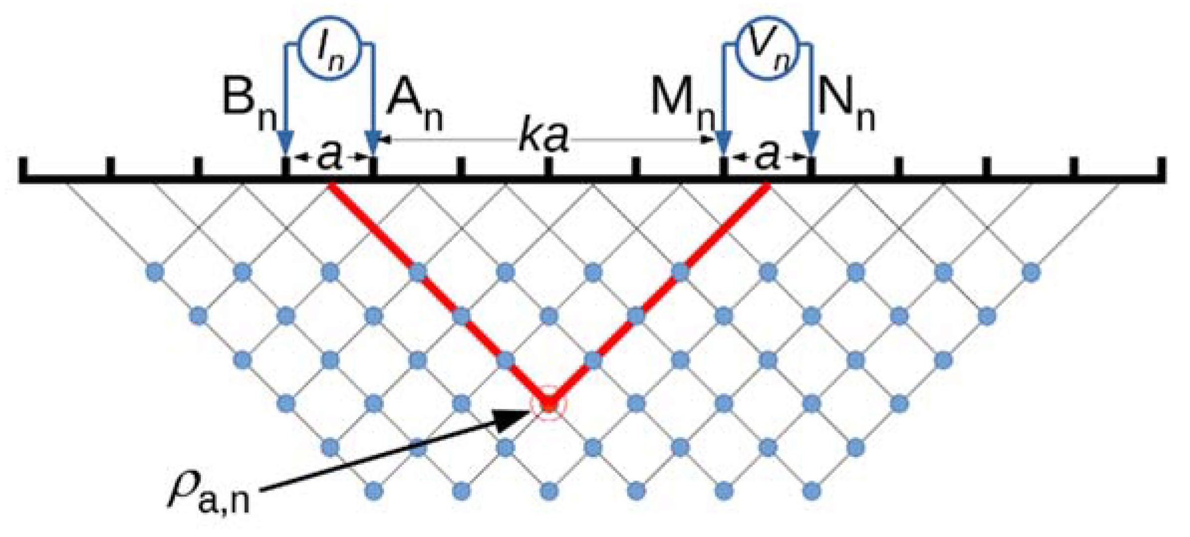
To illustrate the peculiarities of the new E-PERTI approach, we consider at first an application to a simulated geoelectrical profile obtained by a dipole-dipole (DD) electrode array. Before showing the results of the simulation, we illustrate schematically the characteristics of the DD array and the way to construct a DD apparent resistivity pseudosection (Figure 1). The DD apparent resistivity is calculated using the formula
where In is the intensity of the primary current injected into the ground through the electrodes A and B in the nth position (n = 1,2,…,N), say An and Bn, Vn is the potential difference across the electrodes M and N in the nth position, say Mn and Nn, and K = πak (k + 1)(k + 2) is the DD geometrical factor, where a is the amplitude of the dipoles and k is the sampling integer denoting the increasing distance between the dipoles along the profile. A pseudosection indicates how the apparent resistivity varies with location and depth. For the DD electrode configuration, the data are plotted beneath the midpoint between the dipoles at a depth of half the distance between the dipole centres and then contoured using colour palettes.
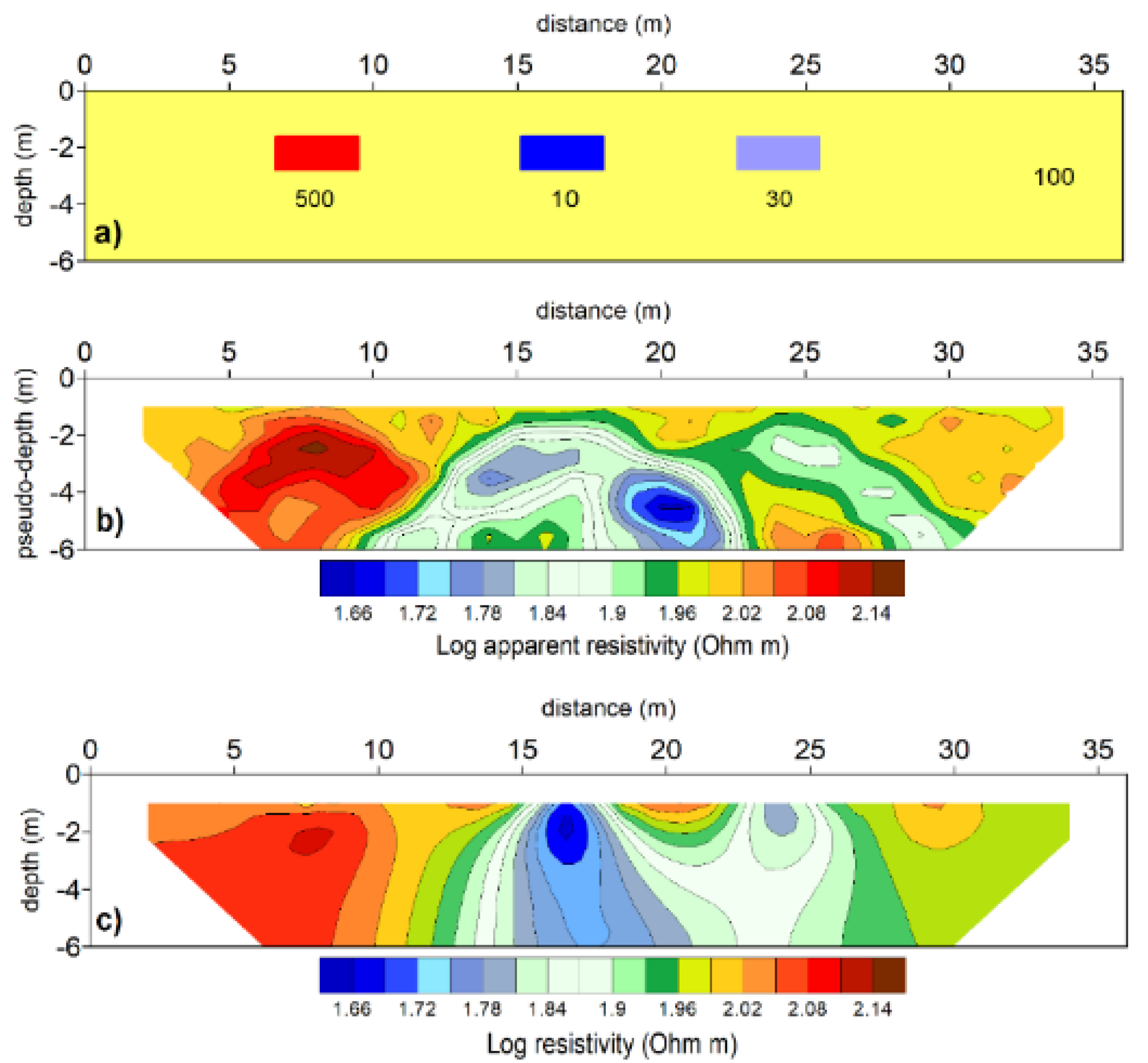
Proceeding now to the simulation, we refer to the 2D three-prism model dealt with in the original PERTI paper [18]. The model, whose cross section is shown in Figure 2a, consists of three infinitely long horizontal prisms with rectangular cross section and resistivities 500 Ωm, 10 Ωm, and 30 Ωm, immersed in a uniform half-space with resistivity 100 Ωm. All of them are 3 m wide and 1.3 m high with the top surfaces placed at 1.5 m of depth. A 36-m long profile is considered using a dipole-dipole (DD) array with fixed 1 m amplitude of both current and potential dipoles. The corresponding apparent resistivity pseudosection contaminated by a 5% random noise is shown in Figure 2b. The resistivity section obtained with the original PERTI method is also plotted in Figure 2c. Mathematical details about the calculation of the Frechet derivative for a dipolar device can be found in [18].
4.1. Random Nq Tests from N-Dimensional Pseudosection Space
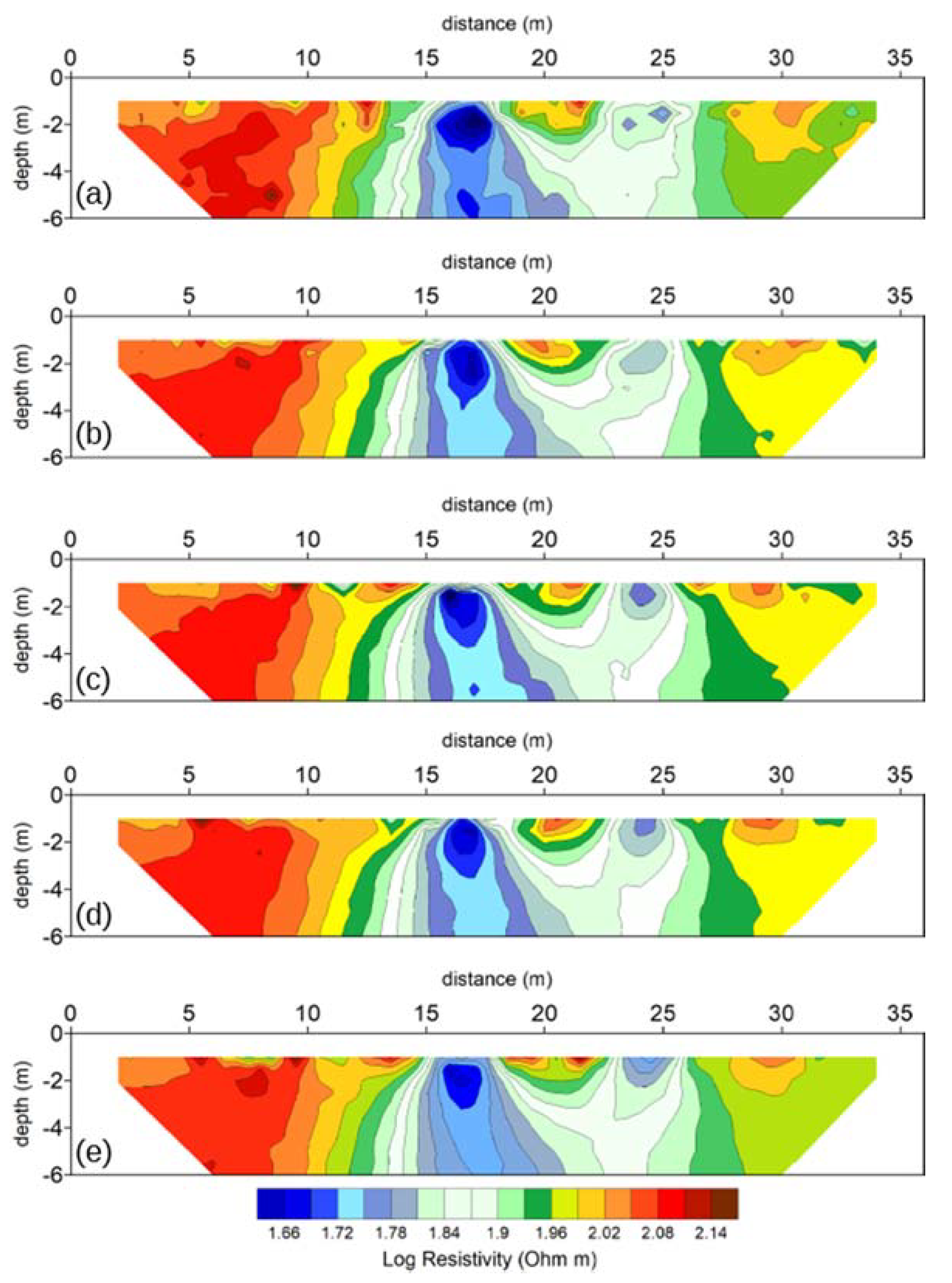
Facing now with the E-PERTI approach, we show the result that can be achieved by randomly extracting Nq data (tests) from the whole set of N data of the pseudosection in Figure 2b. In Figure 3 there are reported from top to bottom the resistivity sections resulting from averaging point by point the resistivity values obtained by the PERTI inversion scheme applied to 20 randomly extracted sets of Nq = 50 (Figure 3a), Nq = 100 (Figure 3b), Nq = 150 (Figure 3c), Nq = 200 (Figure 3d) and Nq = 250 (Figure 3e) tests from the N = 295 starting data set.
In all of the sections in Figure 3, a jagged course of the contour lines is observed, visibly weakening as Nq increases. The presence of the three targets is better delineated with increasing Nq, mostly that of the central body. Worth noting is the relative stable position of the three main nuclei in the sequence of sections, unlike other rather wandering nuclei, mainly in the topmost depth level. This allows giving a statistical relevance to the final choice of the most probable targets with respect to artifacts.
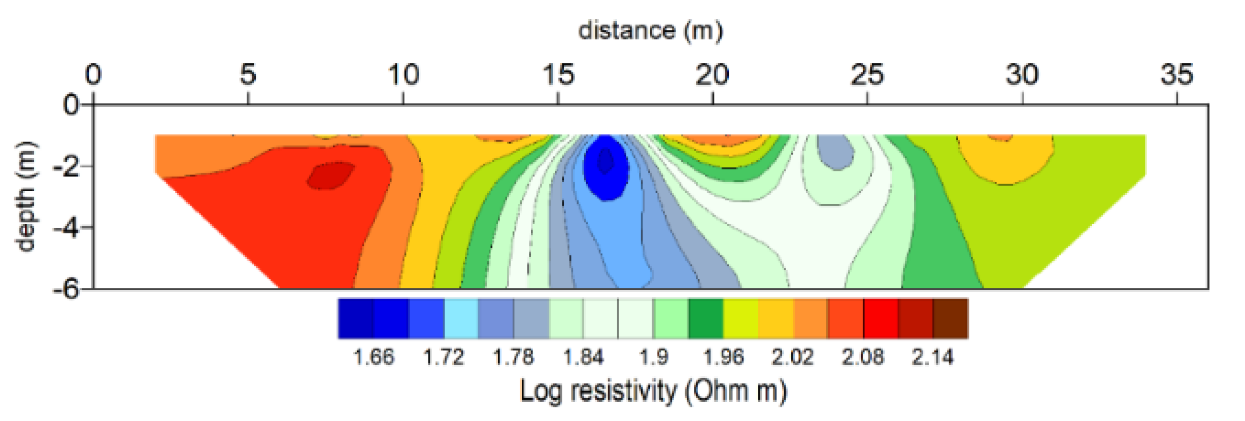
To conclude this first synthetic experiment, Figure 4 provides the result of the least squares linear best fitting over the estimated resistivities, point by point. The final E-PERTI section, which shows a quite smooth behaviour of the contour lines, tends to overlap the section of the original PERTI, shown in Figure 2c. The computational cost for processing both sections (Figure 2c and Figure 4) is a few seconds and there is no substantial processing speed variation between the two methods.
4.2. Progressive Nq Tests by Vertical Scanning
The statistical formulation of the E-PERTI approach allows us to also explore the possibility of a dynamic geoelectric tomography, that is, a dialogue with the dataset to enhance potentially interesting contributions from sequential data subsets, with the purpose to obtain resistivity values that are not influenced by geometrically distant points. Therefore, referring to the pseudosection of Figure 2, we base now the extractions of the Nq subsets on a criterion linked to the depth, i.e., we consider the possibility of a vertical scanning of the pseudosection by selecting subsets with gradually increasing pseudodepths.
In Figure 5, the E-PERTI is applied to the three-prism pseudosection in Figure 2b. The Nq subsets are taken at increasing values of the depth factor k that appears in the definition of the geometrical factor K in Equation (16) (from top to bottom k = 5, k = 7, k = 9, k = 10). As in the original PERTI, the depth of each E-PERTI section is related to the pseudodepth of the corresponding subset.
The last section in Figure 5 depicts the estimates of (m = 1,2,…,M) obtained by the linear best-fit procedure.
As the vertical scanning proceeds from top to bottom, as expected, a gradual weakening of the artifacts is observed, together with a gradual enhancement of the nuclei linked to the three targets. This time the behaviour of the contour lines is quite smooth, since for each section all available data are taken down to the maximum pseudodepth. As previously, the final section appears morphologically quite like that of the original PERTI shown in Figure 2.
4.3. Sequential Nq Tests by Horizontal Scanning
As a further application of dynamic tomography, now we consider a stepwise horizontal scan of the N data space. This approach may be particularly useful when dealing with pseudosections having a horizontal length much higher than the pseudodepth maximum extent. The E-PERTI is thus aimed at analysing subsets of data belonging to contiguous sectors along the pseudosection, as a sort of moving average along the pseudosection.
Referring to the pseudosection in Figure 2, we can extract the Nq tests for example by isolating a 10 m wide data window, moved progressively with a step of 1 m along the profile.
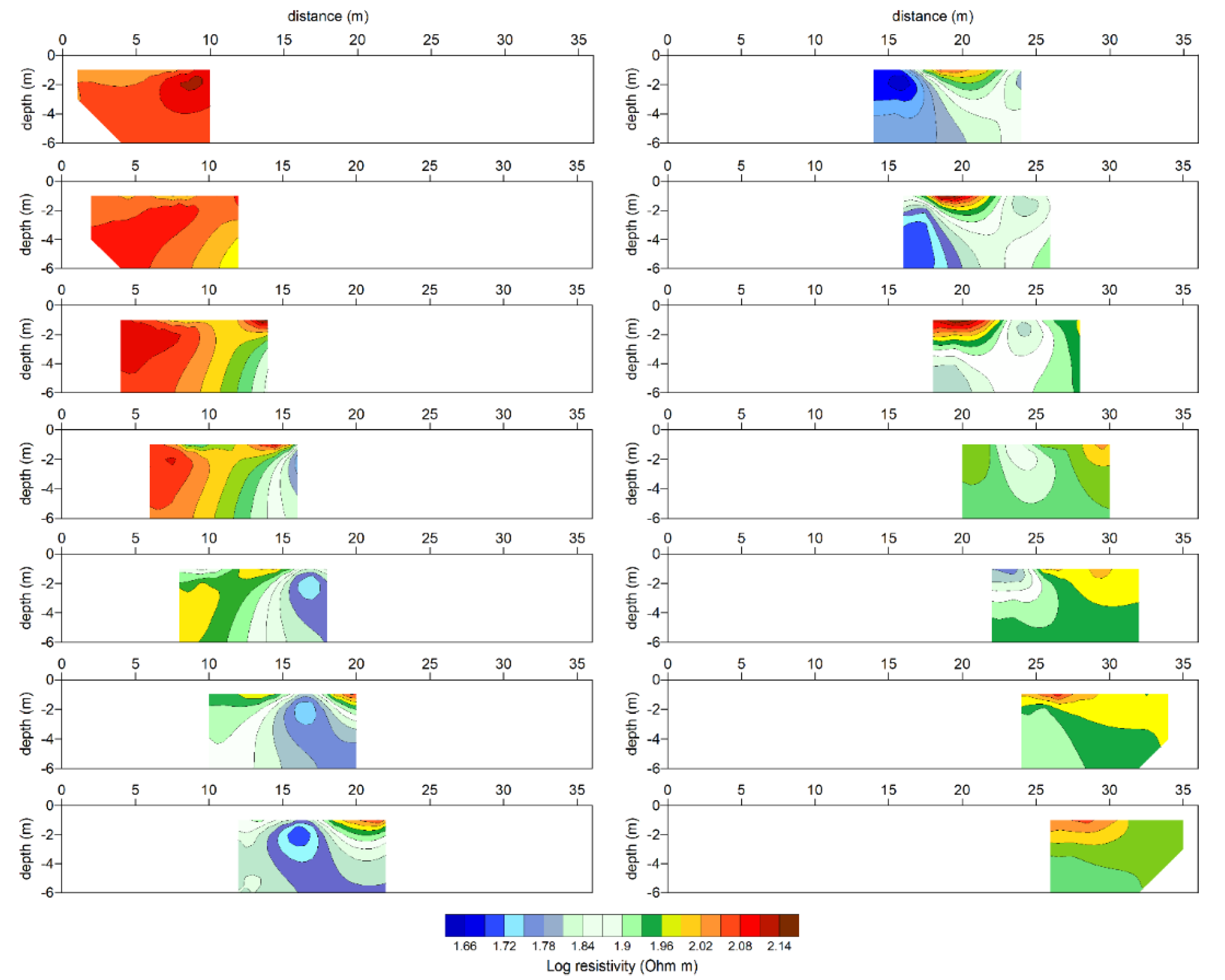
Figure 6 shows the results of this PERTI horizontal scanning, where, for reason of clarity, the PERTI sections are displayed with a 2 m step. This time, an immediate focusing of the targets is obtained when the window runs over them. Again, the contour lines appear very smooth, since for each window all the data in its inside are taken, instead of a random extraction of a lesser number of tests, as done in the first statistical experiment.
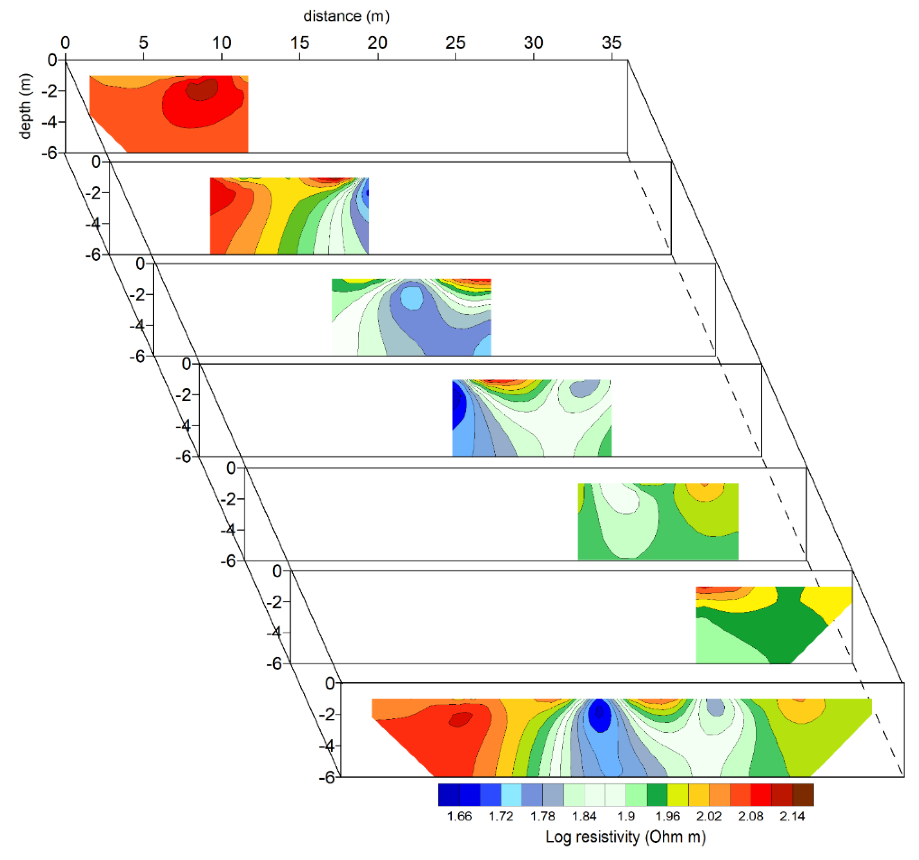
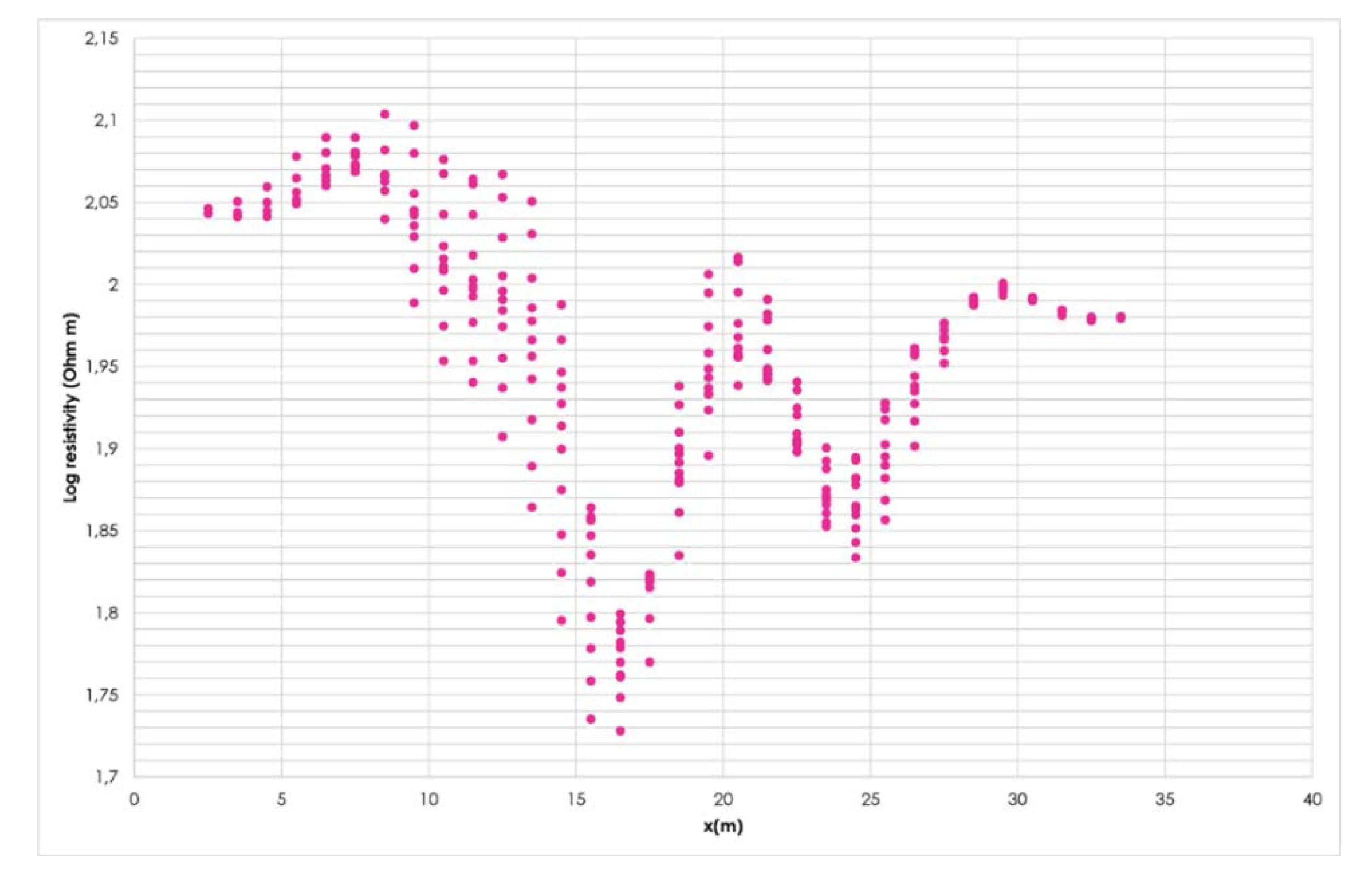
A perspective view of the same PERTI sections of Figure 6, but displayed only every 5 m, is depicted in Figure 7, where the frontmost global section provides the result of the least squares linear best fitting of the resistivities esteemed at attribution points belonging to overlapping windows. Again, the final E-PERTI section does not differ substantially from that shown in Figure 2. It is now time for a general comment about the role of the linear least squares best fit, based on PERTI formula (9) in this paper. In principle, the model resistivities from any inversion process depend on an unpredictable way on profile extent, array setup and local noise level. As an example, Figure 8 shows the resistivity spread point by point along the profile, at 2 m depth from all overlapping segments of Figure 6. Such a spectrum is a clear evidence of why the resistivity spread cannot be disregarded. At the same time, it is a proof of how important is to dispose of a ductile, reliable statistical tool, straight resulting from the adopted inversion process.
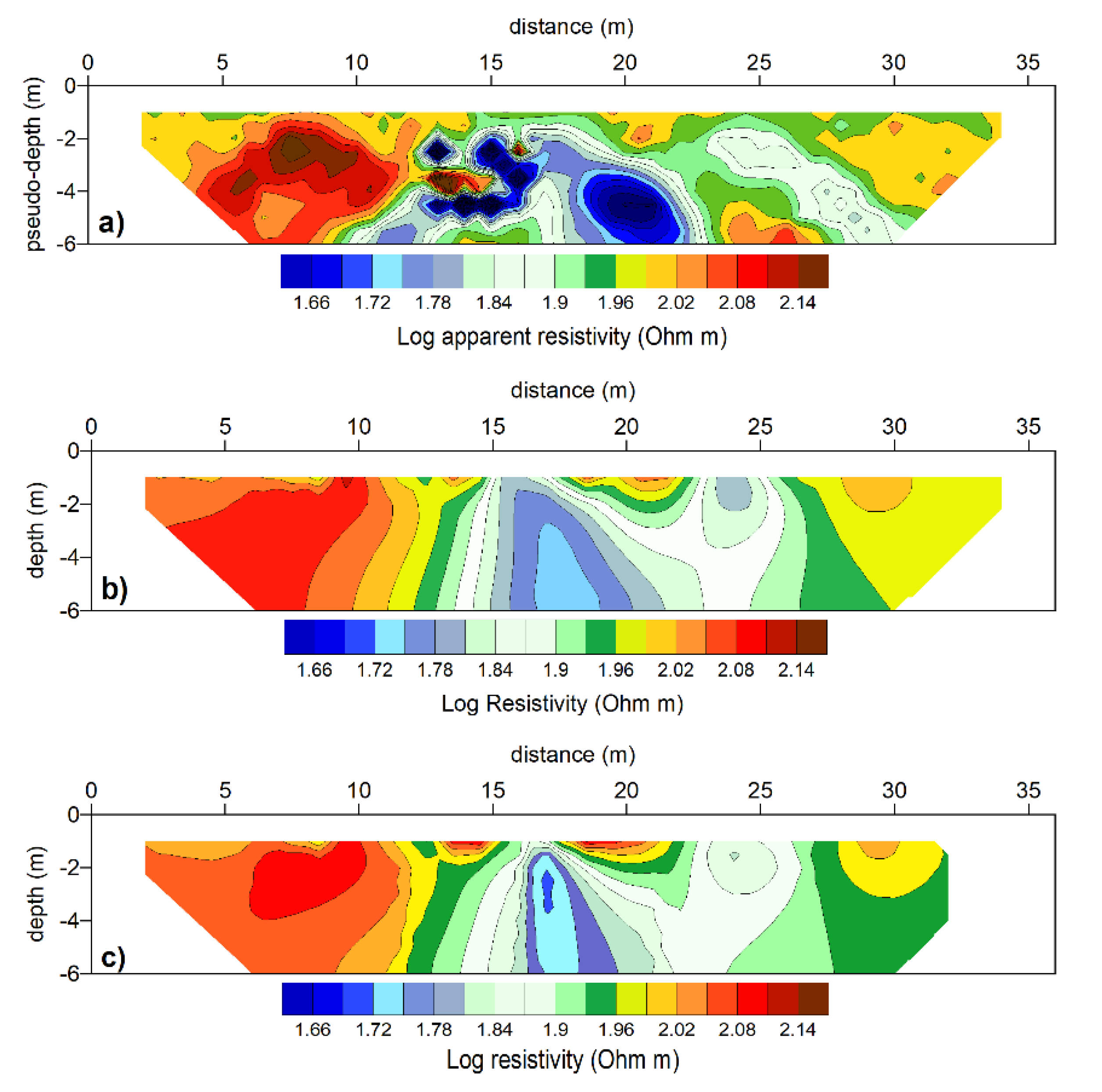
As shown, the major strength of the E-PERTI approach is to dispose of a sound theoretical background for an aware, careful inspection of any dataset. To further explain its practical utility, we consider again the pseudosection in Figure 2, this time by supposing it affected by a 30% random error only in one sector, as in the left half in Figure 9a.
Recognising the presence of noise, one may either be tempted to cut the dirty sector by losing information or try the inversion anyway. With this last choice, using, e.g., the classical PERTI, the resulting tomography would be that shown in Figure 9b. However, adopting the horizontal scanning tool and then using, instead of the standard best fit, a weighted best fit by reducing, e.g., by a factor of 0.7, the resistivity estimates belonging to the windows crossing the corrupted side, the resulting E-PERTI section is that shown in Figure 9c, which is visibly a much better result than that in Figure 9b. Position of the anomaly sources and corresponding values of resistivity appear, in fact, more realistic. Although such a high noise level is probably unusual in many applications, here it has been assumed in order to demonstrate the robustness of the proposed scheme against noise. Even if the use of a weighed best fit may be seen as introducing some subjectivity into the process, this does not conflict with the axioms of probability. In real field cases tests, a careful choice of different weights can help achieving a sounder interpretation of the results. In this context, E-PERTI reveals to be a dynamic tool, and can also be used as a support in other inversion algorithms.
So far, we have shown that the final E-PERTI sections are all morphologically quite like that of the original PERTI shown in Figure 2. Thus, the question could be raised about the real need of such a procedure and its benefits. The point is in principle. Making, e.g., a vertical or horizontal scan in our probabilistic scheme takes on a rigorous statistical character. In other words, an added value is attributed to the best fitting process of all the most probable resistivities. E-PERTI was thus primarily intended to be a tool to give greater emphasis to the probabilistic concept underlying the inversion approach. Moreover, the considerations that in synthesis can be now deduced from the E-PERTI results are that (1) the fitting procedure allows the method to be more robust to noise, and (2) using subsets of the data and vertical/horizontal scanning opens the possibility to optimise data acquisition.
5. Field Example
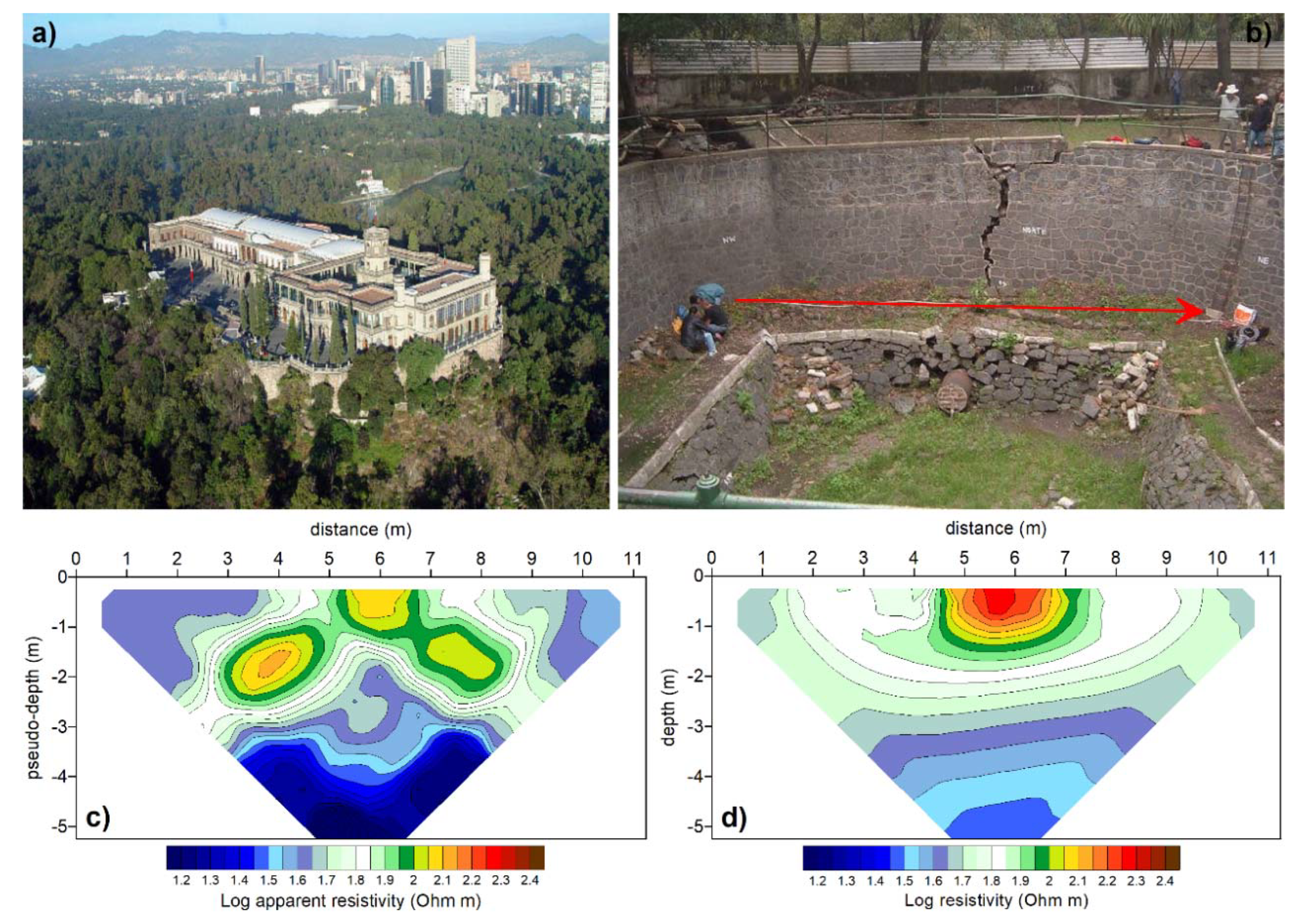
As example of practical application of the E-PERTI approach, we show the results from a field test carried out inside the Baths of Moctezuma, in the ancient Chapultepec Park on the Chapulín hill in Mexico City (Figure 10a). The Baths of Moctezuma (Figure 10b) were containers or cisterns for storing water, built in the pre-Columbian period in the fifteenth century, which were used to channel the water from the springs located in this area toward the centre of the ancient city of Tenochtitlan. Here, one of the metal pipes for conveying the water into the tank is clearly visible.
As part of a wider project of knowledge of the hydraulic system of the castle, an essay was carried out to test the resolution capability of geoelectrics over a small sized target (0.4 m of diameter) buried at very shallow depth (less than 1 m). A DD profile was thus measured using 16 electrodes spaced apart 0.75 m, which allowed to collect 91 apparent resistivity data. The corresponding apparent resistivity pseudosection and the classical PERTI section are shown in Figure 10c,d, respectively.
In the apparent resistivity pseudosection, in correspondence of the pipe, an inverted V-shaped anomaly is visible, which in the PERTI section is converted into the image of a shallow high resistivity body with circular section.
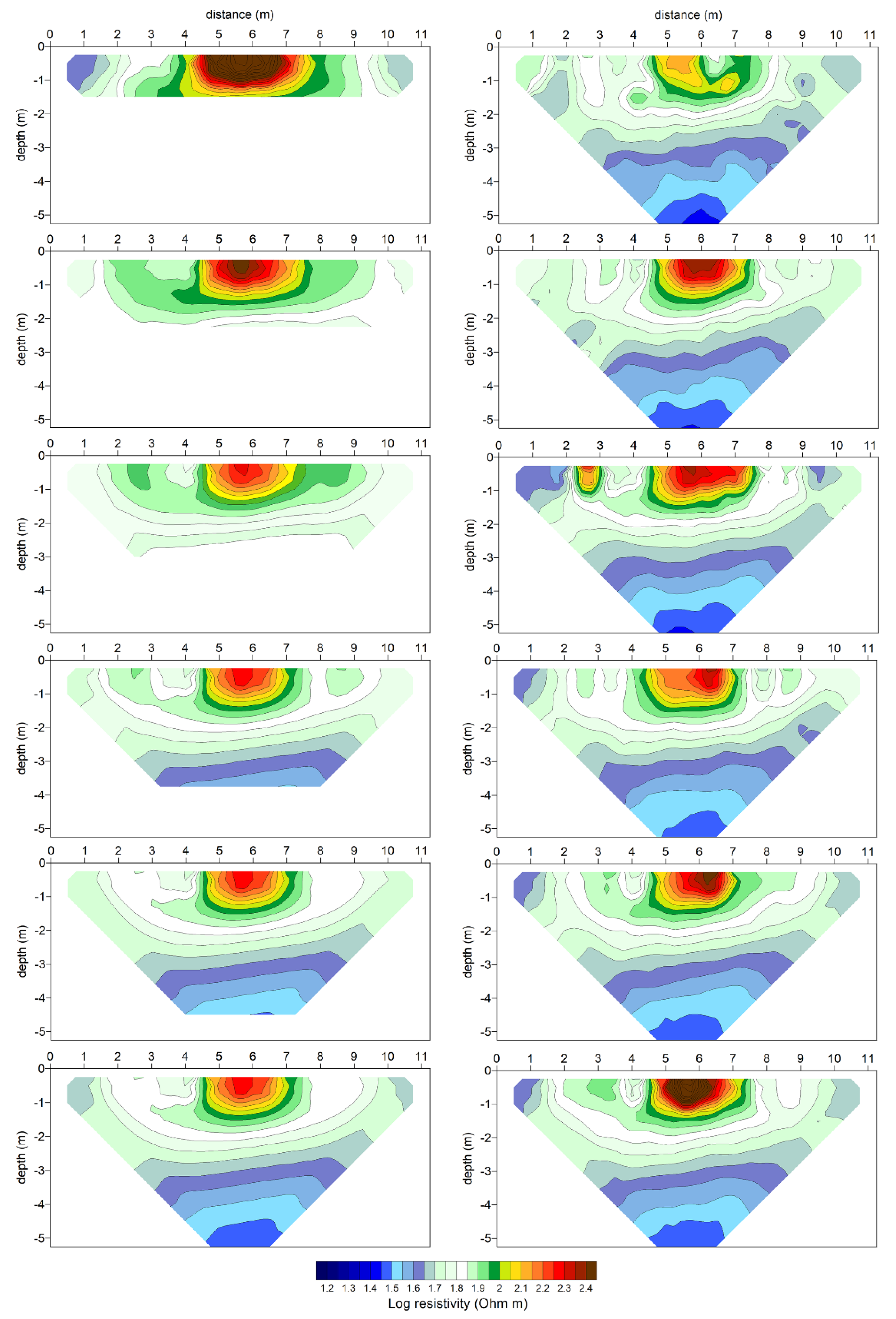
The left-hand column in Figure 11, shows the progressive PERTI sections using the Nq tests depth scanning approach, while the right-hand column shows the sequence of sections, obtained by averaging point by point 10 PERTI sections (for each Nq, 10 data sets were used) elaborated using randomly extracted Nq data (tests) from the N = 91 starting dataset (from top to bottom Nq = 15, Nq = 30, Nq = 45, Nq = 60, Nq = 75 and Nq = 90).
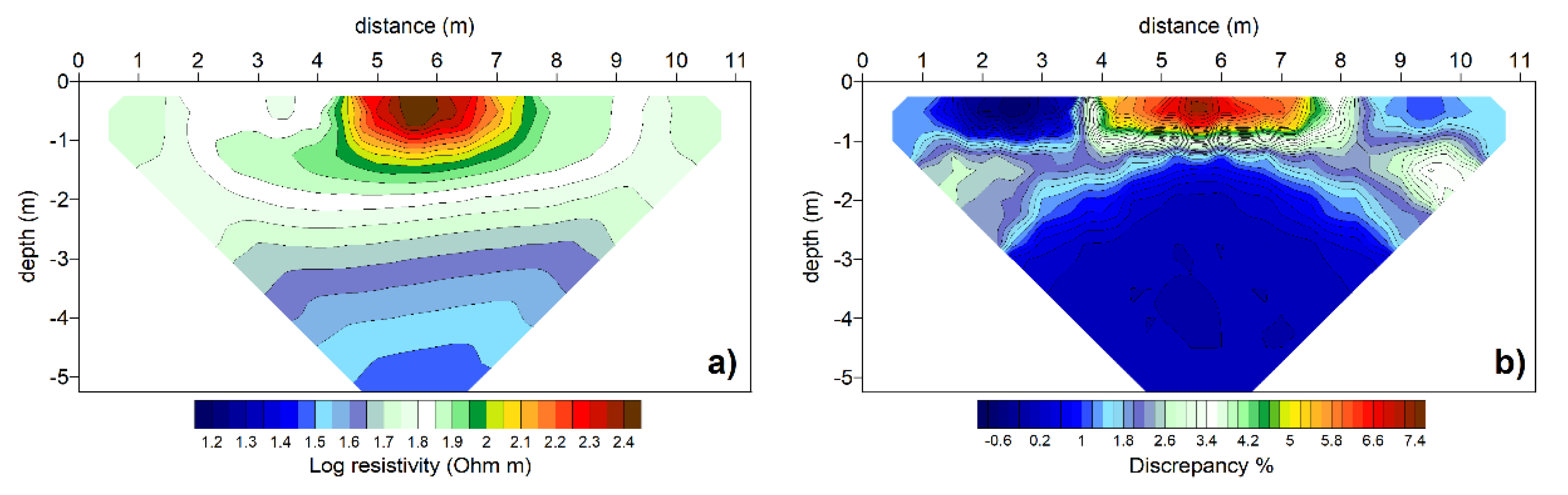
At last, Figure 12a shows the final E-PERTI section, resulting from the least squares linear best fitting applied point by point over the whole set of estimated resistivities from both columns of Figure 11. The E-PERTI section, although very similar to the original PERTI section, at a closer examination displays an improved image of the inner highest resistivity nucleus attributable to the real shape of the pipe.
To make this result more explicit, the section in Figure 12b shows the behaviour of the percent discrepancy factor, calculated at each point as the difference between the resistivity value in the E-PERTI section of Figure 12a and that in the PERTI section of Figure 10d, normalised with respect to the latter. The slightly stronger resistivity contrast that emerges in the section in Figure 12a between the top central nucleus and the surrounding material is thus accepted as a better imaging of the expected contrast between the pipe with adjacent disjointed stony blocks and the surrounding wet fine-grained soil (see Figure 10, intermediate section).
6. Discussion
The motivations behind this work were the good results obtained so far from the application of the PERTI method to a great variety of field cases. Leaving aside the advantages of PERTI, already mentioned in this work, it is now worth spending a few words on those aspects of weakness, which are indeed common to all inversion methods, and are substantially linked to the negative influences produced by the presence of both random and systematic noise on geoelectrical data. Mainly for this last type of noise, in fact, unless there are aprioristic interventions by the interpreter, by their subjective nature and therefore questionable in principle, an uncritical inversion process is generally not able to filter out artefacts entirely, which therefore may often be valued as targets. Many authors recommend using reciprocal data to characterise noise. Reciprocals are able to characterise random noise, and to some extent systematic noise since the current electrodes are not the same. This allows to identify objectively data points with higher noise level and to weigh them during inversion [35,36,37,38].
Reducing the negative influence of noise is thus one of the reasons why the possibility of extending the PERTI tool has been investigated, by introducing the statistical analysis of the behaviour of subsets of data extracted from the original dataset. The relevant aspect of this analysis is that the same PERTI formula, allowing to estimate resistivity in all points of the surveyed space, directly adapts to a statistical linear least-squares best fit. This allows giving a statistical relevance to the recognition of target bodies against artefacts.
The simulations have shown that it is in fact possible to distinguish an artefact from a target, by exploiting from the statistical point of view the quite variable character in intensity and position of the images of the former compared to the stability of the latter. For example, the most classic of the systematic disturbances observed are the so-called reverse V-shaped effects, like that visible in the field pseudosection of Figure 10, or more generally the electrode effects, to which the dipole–dipole device is extremely sensitive. We have shown that in the statistical process of random selection of data subsets, it is possible to recognise the presence of artefacts because of their variability in shape and intensity. Similarly, by the depth progressive scanning statistical procedure, as it proceeds from top to bottom, a gradual fading of these artefacts has also been observed. Therefore, recognised as such, one can try to weaken their influence a posteriori, preserving the information content, e.g., by assigning in any of the elaborations discussed above a low weight to those extracted data that belong to a corrupted dataset sector. An example of this further elaboration is shown in Figure 13.
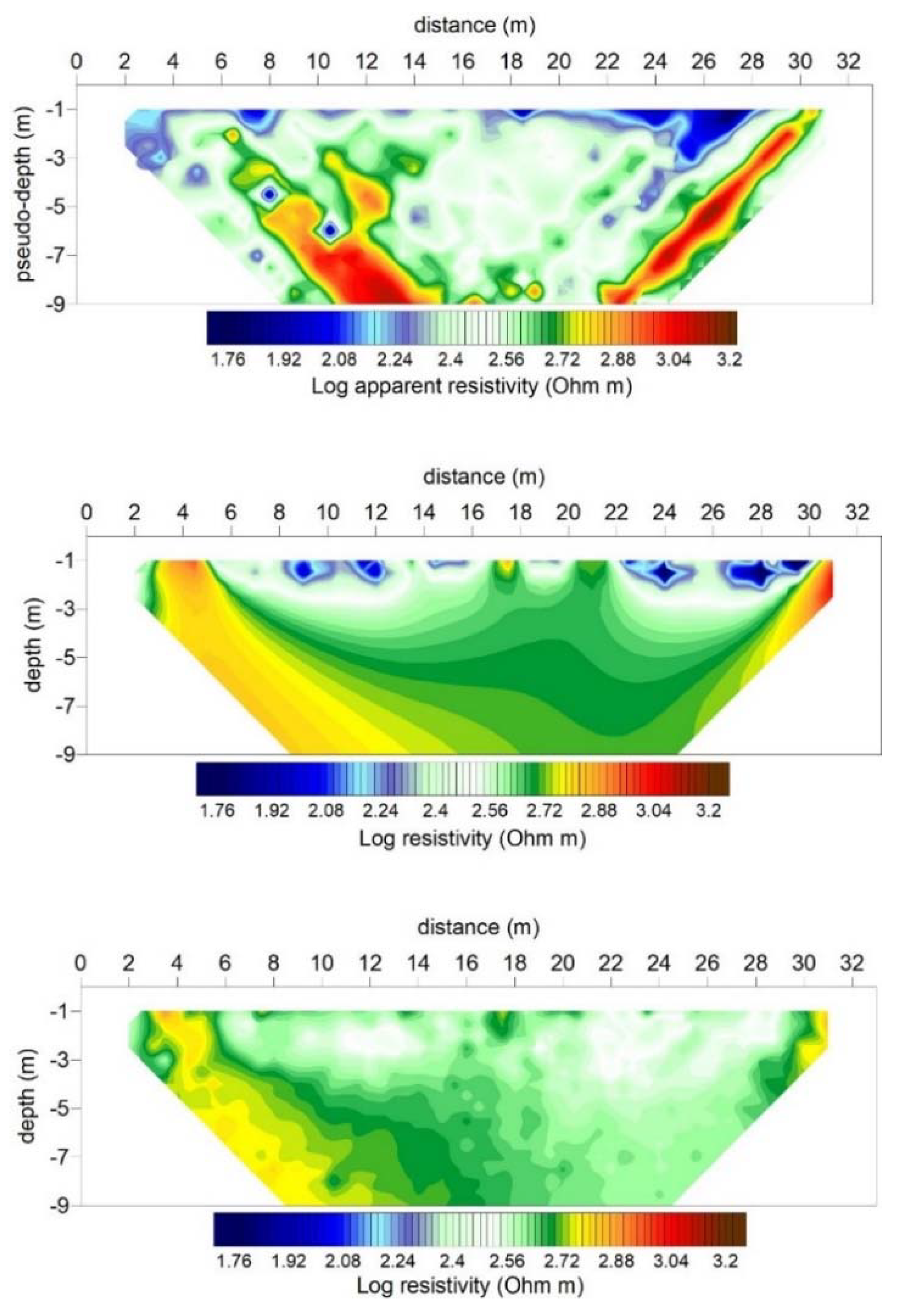
The top section in Figure 13 represents a DD field pseudosection, measured in the archaeological park of Petra (Jordan) in order to check for the presence of a tomb, hypothesised buried inside the local sandstone subsoil. An evident dragging electrode effect, the high elongated resistive zone, is visible at the right-hand margin of the pseudosection, and to a lesser extent another one is present also at the left-hand side. The picture in the middle depicts the classical PERTI section elaborated from the whole original dataset, where the corrupting effect appears largely magnified. Finally, the lower section represents the E-PERTI section derived by a linear best-fit procedure applied to sets of random Nq tests from the original N-dimensional top pseudosection, after damping the influence of the electrode effects. A 20% reduction factor has been applied to all those apparent resistivity values that, after extraction of the Nq tests, resulted in at least 3 points to the corrupted strips. In the final E-PERTI section we now observe that there are not resistive zones on the right part anymore, what seems to exclude the presence of a tomb, which was expected to be a highly resistive target inside a less resistive background. This exercise was done to show the possibility of using E-PERTI to distribute different weights always in a probabilistic key.
7. Conclusions
To conclude we wish now to stress the rationale of the PERTI method, which seems to provide an interesting theoretical framework for interpretation. Although it is not intrinsically better than regularised inversion in terms of imaging, nevertheless it allows to infer a wide variety of statistical outcomes from geoelectrical datasets, permitted by the probabilistic paradigm upon which it is based.
Since modelling is in principle the search for invariants from datum intrinsic variability, probability and statistics presently seemed to us proper tools to help reveal the physical properties of a hidden target.
Bernoulli’s conceptual scheme has been assumed to comply with any resistivity dataset, which allowed a multiplicity of mutually independent subsets to be extracted and analysed singularly. A standard least squares procedure has at last been adopted for the statistical determination of the model resistivity at each point of the surveyed volume as the slope of a linear equation that relates the multiplicity of the resistivity estimates to the extracted data subsets.
The simulations and examples provided in this paper now allow us to state that the E-PERTI fitting procedure reveals more robust to noise than the original PERTI tool, and that the technique of extraction of subsets of the data for both random and vertical/horizontal scanning of the investigated volume open the possibility to optimise the data acquisition process.
At last, we let observe that in all the synthetic and field cases dealt with in this paper, for the sake of conciseness and simplicity we have considered only the dipole–dipole array, limitedly to the widely used 2D profiling technique. Needless to say, the principles of the PERTI method recalled in Section 2, as well as the extension developed in Section 3 are completely general, valid for any electrode device and for 3D applications.
Author Contributions
Conceptualization, M.C., P.M. and D.P.; Data curation, M.C., P.M. and D.P.; Formal analysis, M.C., P.M. and D.P.; Methodology, M.C., P.M. and D.P.; Software, M.C., P.M. and D.P.; Validation, M.C., P.M. and D.P.; Writing—original draft, M.C., P.M. and D.P.; Writing—review & editing, M.C., P.M. and D.P. All authors have read and agreed to the published version of the manuscript.
Funding
This research received no external funding.
Acknowledgments
The authors wish to express their gratitude to the three anonymous referees and the Editor Thomas Hermans for their valuable suggestions, which have helped to improve the manuscript.
Conflicts of Interest
The authors declare no conflict of interest.
References
- Loke, M.H.; Barker, R.D. Rapid least-squares inversion of apparent resistivity pseudosections by a quasi-Newton method. Geophys. Prospect. 1996, 44, 131–152. [Google Scholar] [CrossRef]
- Zhou, B. Electrical Resistivity Tomography: A Subsurface-Imaging Technique. In Applied Geophysics with Case Studies on Environmental, Exploration and Engineering Geophysics; Kanli, A.I., Ed.; IntechOpen: London, UK, 2018; pp. 1–16. [Google Scholar] [CrossRef] [Green Version]
- Andersen, K.E.; Brooks, S.P.; Hansen, M.B. Bayesian inversion of geoelectrical resistivity data. J. R. Stat. Soc. Ser. B (Stat. Methodol.) 2003, 65, 619–642. [Google Scholar] [CrossRef] [Green Version]
- Galetti, E.; Curtis, A. Transdimensional electrical resistivity tomography. J. Geophys. Res. Solid Earth 2018, 123, 6347–6377. [Google Scholar] [CrossRef]
- Ramirez, A.L.; Nitao, J.J.; Hanley, W.G.; Aines, R.; Glaser, R.E.; Sengupta, S.K.; Dyer, K.M.; Ickling, T.L.; Daily, W.D. Stochastic inversion of electrical resistivity changes using a Markov Chain Monte Carlo approach. J. Geophys. Res. Solid Earth 2005, 110. [Google Scholar] [CrossRef] [Green Version]
- Tso, C.-H.M.; Kuras, O.; Wilkinson, P.B.; Uhlemann, S.; Chambers, J.E.; Meldrum, P.I.; Graham, J.; Sherlock, E.F.; Binley, A. Improved characterization and modelling of measurement errors in electrical resistivity tomography (ERT) surveys. J. Appl. Geophys. 2017, 146, 103–119. [Google Scholar] [CrossRef] [Green Version]
- Patella, D. Introduction to ground surface self-potential tomography. Geophys. Prospect. 1997, 45, 653–681. [Google Scholar] [CrossRef]
- Mauriello, P.; Patella, D. Resistivity anomaly imaging by probability tomography. Geophys. Prospect. 1999, 47, 411–429. [Google Scholar] [CrossRef]
- Mauriello, P.; Patella, D. Resistivity tensor probability tomography. Prog. Electromagn. Res. B 2008, 8, 129–146. [Google Scholar] [CrossRef] [Green Version]
- Mauriello, P.; Patella, D. Geoelectrical anomalies imaged by polar and dipolar probability tomography. Prog. Electromagn. Res. 2008, 87, 63–88. [Google Scholar] [CrossRef] [Green Version]
- Alaia, R.; Patella, D.; Mauriello, P. Imaging multipole self- potential sources by 3D probability tomography. Prog. Electromagn. Res. B 2009, 14, 311–339. [Google Scholar] [CrossRef] [Green Version]
- Alaia, R.; Patella, D.; Mauriello, P. Application of geoelectrical 3D probability tomography in a test-site of the archaeological park of Pompei (Naples, Italy). J. Geophys. Eng. 2008, 5, 67–76. [Google Scholar] [CrossRef]
- Compare, V.; Cozzolino, M.; Mauriello, P.; Patella, D. Resistivity probability tomography at the Castle of Zena (Italy). Eurasip J. Image Video Process. 2009, 1–9. [Google Scholar] [CrossRef] [Green Version]
- Minelli, A.; Cozzolino, M.; Di Nucci, A.; Guglielmi, S.; Giannantonio, M.; D’Amore, D.; Pittoni, E.; Groot, A.M. The prehistory of the Colombian territory: The results of the Italian archaeological investigation on the Checua site (Municipality of Nemocòn, Cundinamarca Department). J. Biol. Res. 2012, 85, 94–97. [Google Scholar] [CrossRef]
- Compare, V.; Cozzolino, M.; Mauriello, P.; Patella, D. Three- dimensional resistivity probability tomography at the prehistoric site of Grotta Reali (Molise, Italy). Archaeol. Prospect. 2009, 16, 53–63. [Google Scholar] [CrossRef]
- Compare, V.; Cozzolino, M.; Di Giovanni, E.; Mauriello, P. Examples of resistivity tomography for cultural heritage management. In Near Surface 2010-16th European Meeting of Environmental and Engineering Geophysics; European Association of Geoscientists and Engineers, EAGE: Amsterdam, The Netherlands, 2010. [Google Scholar] [CrossRef]
- Valente, E.; Ascione, A.; Ciotoli, G.; Cozzolino, M.; Porfido, S.; Sciarra, A. Do moderate magnitude earthquakes generate seismically induced ground effects? The case study of the Mw = 5.16, 29th December 2013 Matese earthquake (southern Apennines, Italy). Int. J. Earth Sci. 2018, 107, 517–537. [Google Scholar] [CrossRef] [Green Version]
- Mauriello, P.; Patella, D. A data-adaptive probability-based fast ERT inversion method. Prog. Electromagn. Res. 2009, 97, 275–290. [Google Scholar] [CrossRef] [Green Version]
- Blaschek, R.; Hördt, A.; Kemna, A. A new sensitivity-controlled focusing regularization scheme for the inversion of induced polarization data based on the minimum gradient support. Geophysics 2008, 73, F45–F54. [Google Scholar] [CrossRef]
- Zhdanov, M.S.; Tolstaya, E. Minimum support nonlinear parametrization in the solution of a 3D magnetotelluric inverse problem. Inverse Probl. 2004, 20, 937–952. [Google Scholar] [CrossRef]
- Loke, M.H.; Acworth, I.; Dahlin, T. A comparison of smooth and blocky inversion methods in 2D electrical imaging surveys. Explor. Geophys. 2003, 34, 182–187. [Google Scholar] [CrossRef]
- Hermans, T.; Kemna, A.; Nguyen, F. Covariance-constrained difference inversion of time-lapse electrical resistivity tomography data. Geophysics 2016, 81, E311–E322. [Google Scholar] [CrossRef] [Green Version]
- Amato, V.; Cozzolino, M.; De Benedittis, G.; Di Paola, G.; Gentile, V.; Giordano, C.; Marino, P.; Rosskopf, C.M.; Valente, E. An integrated quantitative approach to assess the archaeological heritage in highly anthropized areas: The case study of Aesernia (southern Italy). Acta Imeko 2016, 5, 33–43. [Google Scholar] [CrossRef]
- Cozzolino, M.; Di Giovanni, E.; Mauriello, P.; Vanni Desideri, A.; Patella, D. Resistivity tomography in the Park of Pratolino at Vaglia (Florence, Italy). Archaeol. Prospect. 2012, 19, 253–260. [Google Scholar] [CrossRef]
- Cozzolino, M.; Mauriello, P.; Patella, D. Resistivity Tomography Imaging of the substratum of the Bedestan Monumental Complex at Nicosia, Cyprus. Archaeometry 2014, 56, 331–350. [Google Scholar] [CrossRef] [Green Version]
- Cozzolino, M.; Longo, F.; Pizzano, N.; Rizzo, M.L.; Voza, O.; Amato, V.A. Multidisciplinary Approach to the Study of the Temple of Athena in Poseidonia-Paestum (Southern Italy): New Geomorphological, Geophysical and Archaeological Dat. Geosciences 2019, 9, 324. [Google Scholar] [CrossRef] [Green Version]
- Cozzolino, M.; Caliò, L.M.; Gentile, V.; Mauriello, P.; Di Meo, A. The Discovery of the Theater of Akragas (Valley of Temples, Agrigento, Italy): An Archaeological Confirmation of the Supposed Buried Structures from a Geophysical Survey. Geosciences 2020, 10, 161. [Google Scholar] [CrossRef]
- Cozzolino, M.; Baković, M.; Borovinić, N.; Galli, G.; Gentile, V.; Jabučanin, M.; Mauriello, P.; Merola, P.; Živanović, M. The contribution of geophysics to the knowledge of the hidden archaeological heritage of Montenegr. Geosciences 2020, 10, 187. [Google Scholar] [CrossRef]
- Di Giuseppe, M.G.; Troiano, A.; Fedele, A.; Caputo, T.; Patella, D.; Troise, C.; De Natale, G. Electrical resistivity tomography imaging of the near-surface structure of the Solfatara crater, Campi Flegrei (Naples, Italy). Bull. Volcanol. 2015, 77, 27. [Google Scholar] [CrossRef]
- Cozzolino, M.; Mauriello, P.; Moisidi, M.; Vallianatos, F. A Probability Electrical Resistivity Tomography Imaging of complex tectonic features in the Kissamos and Paleohora urban areas, Western Crete (Greece). Ann. Geophys. 2019, 62. [Google Scholar] [CrossRef] [Green Version]
- Gnedenko, B.V. Kurs Teorii Verojatnostej, Mir, Moscow; Published in Italian as Teoria della Probabilità; Editori Riuniti: Rome, Italy, 1979. [Google Scholar]
- Uhlemann, S.; Wilkinson, P.B.; Maurer, H.; Wagner, F.M.; Johnson, T.C.; Chambers, J.E. Optimized survey design for electrical resistivity tomography: Combined optimization of measurement configuration and electrode placement. Geophys. J. Int. 2018, 214, 108–121. [Google Scholar] [CrossRef]
- Wilkinson, P.B.; Chambers, J.E.; Meldrum, P.I.; Ogilvy, R.D.; Caunt, S. Optimization of Array Configurations and Panel Combinations for the Detection and Imaging of Abandoned Mineshafts using 3D Cross-Hole Electrical Resistivity Tomography. J. Environ. Eng. Geophys. 2006, 11, 213–221. [Google Scholar] [CrossRef] [Green Version]
- Stummer, P.; Maurer, H.; Green, A.G. Experimental design: Electrical resistivity data sets that provide optimum subsurface information. Geophysics 2004, 69, 120–139. [Google Scholar] [CrossRef]
- LaBrecque, D.J.; Miletto, M.; Daily, W.; Ramirez, A.; Owen, E. The effects of noise on Occam’s inversion of resistivity tomography data. Geophysics 1996, 61, 538–548. [Google Scholar] [CrossRef]
- Slater, L.; Binley, A.M.; Daily, W.; Johnson, R. Cross-hole electrical imaging of a controlled saline tracer injection. J. Appl. Geophys. 2000, 44, 85–102. [Google Scholar] [CrossRef]
- Koestel, J.; Kemna, A.; Javaux, M.; Binley, A.; Vereecken, H. Quantitative imaging of solute transport in an unsaturated and undisturbed soil monolith with 3-D ERT and TDR. Water Resour. Res. 2008, 44, W12411. [Google Scholar] [CrossRef] [Green Version]
- Lesparre, N.; Nguyen, F.; Kemna, A.; Robert, T.; Hermans, T.; Daoudi, M.; Flores-Orozco, A. A new approach for time-lapse data weighting in electrical resistivity tomography. Geophysics 2017, 82, E325–E333. [Google Scholar] [CrossRef]
Figure 1.
Schematic depiction of the characteristics of a dipole-dipole electrode device used to perform a 2D geoelectrical profile and the rule used to construct an apparent resistivity pseudosection.
Figure 1.
Schematic depiction of the characteristics of a dipole-dipole electrode device used to perform a 2D geoelectrical profile and the rule used to construct an apparent resistivity pseudosection.

Figure 2.
A synthetic test: (a) assigned 2D three-prism model, (b) simulated pseudosection, (c) model reconstruction by the original PERTI method.
Figure 2.
A synthetic test: (a) assigned 2D three-prism model, (b) simulated pseudosection, (c) model reconstruction by the original PERTI method.

Figure 3.
Average sections, obtained by averaging point by point 20 PERTI sections elaborated using randomly extracted Nq data (tests) from the N = 295 starting dataset. Nq = 50 (a), Nq = 100 (b), Nq = 150 (c), Nq = 200 (d) and Nq = 250 (e).
Figure 3.
Average sections, obtained by averaging point by point 20 PERTI sections elaborated using randomly extracted Nq data (tests) from the N = 295 starting dataset. Nq = 50 (a), Nq = 100 (b), Nq = 150 (c), Nq = 200 (d) and Nq = 250 (e).

Figure 4.
Section resulting from the estimation of with a linear best-fit procedure applied point by point to the resistivity values belonging to the PERTI sections in Figure 2.
Figure 4.
Section resulting from the estimation of with a linear best-fit procedure applied point by point to the resistivity values belonging to the PERTI sections in Figure 2.

Figure 5.
Extractions of the Nq tests in depth (from top to bottom k = 5, k = 7, k = 9, k = 10) and estimation of with linear best-fit procedure (last section).
Figure 5.
Extractions of the Nq tests in depth (from top to bottom k = 5, k = 7, k = 9, k = 10) and estimation of with linear best-fit procedure (last section).

Figure 6.
Extraction of the Nq tests by a stepwise displacement of 2 m of a 10 m wide data window along the array axis. The reduced sections are classical PERTI results over the whole set of tests within each window.
Figure 6.
Extraction of the Nq tests by a stepwise displacement of 2 m of a 10 m wide data window along the array axis. The reduced sections are classical PERTI results over the whole set of tests within each window.

Figure 7.
A perspective view of the same synthetic experiment as in Figure 6, but with PERTI sections displayed every 5 m along the profile axis, and estimation of with linear best-fit procedure (frontmost section).
Figure 7.
A perspective view of the same synthetic experiment as in Figure 6, but with PERTI sections displayed every 5 m along the profile axis, and estimation of with linear best-fit procedure (frontmost section).

Figure 8.
Example of dispersion of resistivity values at 2 m depth from all overlapping segments of Figure 6, against offset distance x along the entire profile length.
Figure 8.
Example of dispersion of resistivity values at 2 m depth from all overlapping segments of Figure 6, against offset distance x along the entire profile length.

Figure 9.
Pseudosection corresponding to the three-prism model in Figure 2a, corrupted by a 30% random noise in the left side portion (a); classical PERTI section (b); section resulting from the estimation of with a weighted best-fit procedure applied point by point to the resistivity values obtained by a sequential horizontal scanning (c).

Figure 10.
Chapultepec castle on the Chapulín hill in Mexico City (a), the Baths of Moctezuma (b) with indication of the survey line, the dipole-dipole (DD) pseudosection (c) and the PERTI section (d).
Figure 10.
Chapultepec castle on the Chapulín hill in Mexico City (a), the Baths of Moctezuma (b) with indication of the survey line, the dipole-dipole (DD) pseudosection (c) and the PERTI section (d).

Figure 11.
Extension of PERTI for the field example of Figure 10 showing progressive Nq tests by vertical scanning (left column) and random Nq tests from the N-dimensional pseudosection space (right column).
Figure 11.
Extension of PERTI for the field example of Figure 10 showing progressive Nq tests by vertical scanning (left column) and random Nq tests from the N-dimensional pseudosection space (right column).

Figure 12.
E-PERTI section resulting from the estimation of with a linear best-fit procedure applied point by point to the resistivity values belonging to the PERTI sections in Figure 11 (a) and discrepancy section between the E-PERTI section in (a) and the classical PERTI section in Figure 10b (b).

Figure 13.
Fading procedure of a systematic noise effect from a field dataset: the DD field pseudosection (upper section), the classical PERTI section (intermediate section), the filtered best-fit E-PERTI section (lower section).
Figure 13.
Fading procedure of a systematic noise effect from a field dataset: the DD field pseudosection (upper section), the classical PERTI section (intermediate section), the filtered best-fit E-PERTI section (lower section).

© 2020 by the authors. Licensee MDPI, Basel, Switzerland. This article is an open access article distributed under the terms and conditions of the Creative Commons Attribution (CC BY) license (http://creativecommons.org/licenses/by/4.0/).
Share and Cite
MDPI and ACS Style
Cozzolino, M.; Mauriello, P.; Patella, D. An Extension of the Data-Adaptive Probability-Based Electrical Resistivity Tomography Inversion Method (E-PERTI). Geosciences 2020, 10, 380. https://doi.org/10.3390/geosciences10100380
AMA Style
Cozzolino M, Mauriello P, Patella D. An Extension of the Data-Adaptive Probability-Based Electrical Resistivity Tomography Inversion Method (E-PERTI). Geosciences. 2020; 10(10):380. https://doi.org/10.3390/geosciences10100380
Chicago/Turabian StyleCozzolino, Marilena, Paolo Mauriello, and Domenico Patella. 2020. "An Extension of the Data-Adaptive Probability-Based Electrical Resistivity Tomography Inversion Method (E-PERTI)" Geosciences 10, no. 10: 380. https://doi.org/10.3390/geosciences10100380
Note that from the first issue of 2016, this journal uses article numbers instead of page numbers. See further details here.