Article

Novel Expressions for the Derivatives of Sixth Kind Chebyshev Polynomials: Spectral Solution of the Non-Linear One-Dimensional Burgers’ Equation

by
Waleed Mohamed Abd-Elhameed
Department of Mathematics, Faculty of Science, Cairo University, Giza 12613, Egypt
Fractal Fract. 2021, 5(2), 53; https://doi.org/10.3390/fractalfract5020053
Submission received: 16 April 2021 / Revised: 30 May 2021 / Accepted: 3 June 2021 / Published: 6 June 2021
(This article belongs to the Section Numerical and Computational Methods)

Abstract

:
This paper is concerned with establishing novel expressions that express the derivative of any order of the orthogonal polynomials, namely, Chebyshev polynomials of the sixth kind in terms of Chebyshev polynomials themselves. We will prove that these expressions involve certain terminating hypergeometric functions of the type 4 F 3 ( 1 ) that can be reduced in some specific cases. The derived expressions along with the linearization formula of Chebyshev polynomials of the sixth kind serve in obtaining a numerical solution of the non-linear one-dimensional Burgers’ equation based on the application of the spectral tau method. Convergence analysis of the proposed double shifted Chebyshev expansion of the sixth kind is investigated. Numerical results are displayed aiming to show the efficiency and applicability of the proposed algorithm.

1. Introduction

Orthogonal polynomials are successfully employed for the numerical solutions of various differential equations. For example, Jacobi polynomials and their special cases are extensively utilized in a variety of papers. Four kinds of Chebyshev polynomials are specific polynomials of the family of Jacobi polynomials. The first and second kinds are ultraspherical polynomials, while the third and fourth kinds are two types of non-symmetric Jacobi polynomials. All four kinds of Chebyshev polynomials have their roles and applications. They are widely investigated from both theoretical and numerical points of view. For example, Kim et al. in [1] established some sums of finite products of the second, third, and fourth kinds. From a practical point of view, a new class of dual-band waveguide filters is introduced based on Chebyshev polynomials of the second kind in [2]. Oloniiju et al. in [3] utilized Chebyshev polynomials of the first kind to obtain a pseudo-spectral solution to a certain multi-dimensional fractional problem.
Among the important orthogonal polynomials are the so-called “generalized ultraspherical polynomials”. These polynomials were investigated by Lashenov in [4]. The generalized ultraspherical polynomials involve two parameters. For specific choices of these parameters, one obtains the standard ultraspherical polynomials. In addition, there are other two special classes of the generalized ultraspherical polynomials, namely, Chebyshev polynomials of the fifth and sixth kinds. These two classes of polynomials were also introduced in the Ph. D. thesis of Jamei [5]. In fact, Jamei, called these polynomials “Chebyshev polynomials” since he could represent them by half-trigonometric expressions. The authors in [6,7] found full trigonometric expressions for these polynomials, so these two kinds of polynomials may be classified as “Chebyshev polynomials” because of their trigonometric expressions, such as the well-known four kinds of Chebyshev polynomials. Recently, fifth and sixth kinds Chebyshev polynomials have been studied theoretically and practically. For example, Abd-Elhameed and Youssri developed new moments and linearization formulas of the sixth kind Chebyshev polynomials in [8]. Moreover, the same authors in [6,7] utilized the fifth and sixth kinds Chebyshev polynomials in handling some types of fractional differential equations. Jafari et al. in [9] utilized a sixth kind collocation algorithm to treat an inverse reaction-diffusion-convection problem. Moreover, in [10], the authors solved a class of non-linear variable-order fractional reaction-diffusion equation based on using the shifted Chebyshev polynomials of the fifth kind. For some other articles concerned with the different kinds of Chebyshev polynomials, see for example [11,12,13,14].
From a numerical point of view, spectral methods have been extensively utilized for obtaining numerical solutions of various differential equations. The fundamental principle behind the implementation of spectral methods is built on expressing the numerical solution as a suitable combination of certain selected polynomials. Extensive attention has been appointed to various types of spectral methods because of their roles in numerical analysis in general, and in the scope of numerical solutions of differential and integral equations in particular. One can consult [15,16,17] for the different applications of spectral methods in various disciplines. There are three celebrated kinds of spectral methods, namely, the Galerkin, tau and collocation methods. Galerkin method is productively applied to some types of differential equations, see for example [18,19,20,21]. Tau method is advantageous in use due to its flexibility, since no need for choosing the basis functions satisfying the underlying initial and boundary conditions unlike the Galerkin method, see for example [22,23,24,25,26]. The collocation method is the most common method in use. It can be applied to all types of differential equations. For some articles that employ collocation methods in the numerical solutions of different types of differential equations, one can be referred to [27,28,29,30,31,32].
The hypergeometric functions are crucial in mathematical analysis and its applications. In fact, they arise in the area of special functions and their applications. Various important formulas of different orthogonal polynomials and special functions may be given in explicit formulas involve hypergeometric functions or generalized hypergeometric functions. It is worthwhile to mention that the duplication, connection and linearization coefficients of Jacobi polynomials and their particular polynomials are expressed in terms of different hypergeometric functions of unit argument. These hypergeometric functions may be reduced in some cases by either standard formulas or through some suitable symbolic algorithms such as Zielberger’s algorithm, see for example [33,34,35].
The problem of determining the coefficients linking the high-order derivatives and repeated integrals of special functions with their original polynomials is of great interest. These coefficients play important parts in spectral methods. They serve in the numerical solutions of linear and non-linear differential equations. These coefficients are often expressed in terms of hypergeometric functions of unit argument which can be summed in particular cases. For example, the authors in [36] established expressions of the derivatives of the fifth kind Chebyshev polynomials and they proved that these expressions involve hypergeometric functions of the type 4 F 3 ( 1 ) . Furthermore, in the two papers [18,37], the authors developed new formulas for the high-order derivatives and repeated integrals of Chebyshev polynomials of the third and fourth kinds and utilized the developed formulas for treating some special types of differential equations. Additionally, the linearization problems of different special functions are of fundamental interest in mathematical physics. For some important articles in this direction, one can consult [38,39,40].
The non-linear Burgers’ equation and its modified equations are of interest. There are several authors who treated these types of equations using different numerical algorithms. Some of these methods are: operational matrix method [41], collocation method based on B-splines [42], reproducing kernel function [43], finite difference method [44], modified cubic B-spline differential quadrature method [45], modified cubic B-spline collocation method [46], cubic B-spline differential quadrature methods [47], improvised cubic B-spline collocation method in [48]. On the other hand, some other methods were followed for treating Burgers-type equations. For example, the authors in [49] obtained exact travelling wave solutions for the local fractional two-dimensional Burgers-type equations.
One of the principal goals of this article is to establish new expressions of the high-order derivatives of the sixth kind Chebyshev polynomials. It will be shown that these derivatives can be expressed in terms of hypergeometric functions of the type 4 F 3 ( 1 ) that can be reduced in some specific cases. Another principal goal of this article is to utilize these formulas for obtaining numerical solutions of the non-linear one dimensional Burgers’ equation with the aid of the spectral tau method.
The main reasons for our attention to investigate and employ the class of the Chebyshev polynomials of the sixth kind which is a special class of the generalized ultraspherical polynomials are due to the following reasons:
  • Some of the fundamental formulas concerned with the Chebyshev polynomials of the sixth kind such as the power form representation, inversion formula and the moments formula are not difficult in deriving;
  • Chebyshev polynomials of the sixth kind have a trigonometric representation which simplifies the derivation of some formulas concerned with them;
  • The linearization coefficients of these polynomials were derived before in Reference [8] in an explicit simple expression. These coefficients are crucial in the implementation of our proposed numerical algorithm in the current paper.
The rest of the paper is arranged as follows. In Section 2, an overview on the generalized ultraspherical polynomials and the sixth kind Chebyshev polynomials is given. Section 3 is interested in establishing new expressions of the high-order derivatives of sixth kind Chebyshev polynomials in terms of their original ones. Section 4 is devoted to presenting and analyzing a spectral algorithm for treating the one-dimensional Burgers’ equation based on the application of the spectral tau method. The convergence analysis of the double shifted Chebyshev expansion is investigated in Section 5. Section 6 is concerned with displaying some illustrative examples. At the end of the paper, we give some concluding remarks in Section 7.

2. An Overview on the Generalized Ultraspherical Polynomials and Chebyshev Polynomials of the Sixth Kind

This section is dedicated to presenting an overview on the symmetric polynomials, namely, the generalized ultraspherical polynomials. In addition, we will give some relations and identities concerned with a special class of these polynomials, namely Chebyshev polynomials of the sixth kind.

2.1. An Overview on the Generalized Ultraspherical Polynomials

The generalized monic ultraspherical polynomials are symmetric polynomials that generalize the standard monic ultraspherical polynomials [4]. These polynomials are linked with Jacobi polynomials by the following relation:
R k ( λ , μ ) ( x ) = k 2 ! λ + μ + 1 2 k 2 λ + μ + 1 2 k P k 2 λ , μ 1 2 2 x 2 1 , k even , x k 1 2 ! λ + μ + 1 2 k + 1 2 λ + μ + 1 2 k P k 1 2 λ , μ + 1 2 2 x 2 1 , k odd ,
where P k ( λ , μ ) is the standard Jacobi polynomial of degree k.
The generalized ultraspherical polynomials R k ( λ , μ ) ( x ) are orthogonal polynomials on [ 1 , 1 ] with respect to the weight function w ( x ) = ( 1 x 2 ) λ x μ . Therefore, it is clear that the standard ultraspherical polynomials can be obtained as special ones of the generalized polynomials R k ( λ , μ ) ( x ) for the case corresponding to μ = 0 .
In this paper, we will employ a specific kind of the generalized ultraspherical polynomials R k ( λ , μ ) ( x ) . More precisely, we will consider the case corresponding to λ = 1 2 and μ = 2 . These polynomials are called Chebyshev polynomials of the sixth kind.

2.2. Some Fundamental Properties of Sixth Kind Chebyshev Polynomials

This subsection concentrates on displaying some fundamental properties and relations of Chebyshev polynomials of the sixth kind Y m ( x ) = R m ( 1 2 , 2 ) ( x ) , m 0 . These polynomials are orthogonal on [ 1 , 1 ] with respect to w ( x ) = x 2 1 x 2 . More precisely, we have (see [7])
1 1 x 2 1 x 2 Y m ( x ) Y n ( x ) d x = g m , if   m = n , 0 , if   m n ,
and
g m = π 2 2 m + 3 1 , m even , m + 3 m + 1 , m odd .
The polynomials Y k ( x ) can be generated via the following recurrence relation:
Y k ( x ) = x Y k 1 ( x ) k ( k + 1 ) + ( 1 ) k ( 2 k + 1 ) + 1 4 k ( k + 1 ) Y k 2 ( x ) , Y 0 ( x ) = 1 , Y 1 ( x ) = x , k 2 .
Abd-Elhameed and Youssri in [7] proved that Chebyshev polynomials of the sixth kind have the following trigonometric representation:
Y j cos θ = sin ( j + 2 ) θ 2 j sin 2 θ , j even , sin ( j + 1 ) θ + ( j + 1 ) cos ( θ ) sin ( j + 2 ) θ 2 j + 1 ( j + 1 ) cos 2 ( θ ) sin ( θ ) , j odd .
The following two lemmas display the power form representations of Chebyshev polynomials of the sixth kind and their inversion formulae.
Lemma 1
([8]). If n is a non-negative integer, then the power form representations of Chebyshev polynomials of the sixth kind are given by
Y 2 n ( x ) = Γ n + 3 2 ( 2 n + 1 ) ! k = 0 n ( 1 ) k n k ( k + 2 n + 1 ) ! Γ k + n + 3 2 x 2 n 2 k ,
Y 2 n + 1 ( x ) = Γ n + 5 2 ( 2 n + 2 ) ! k = 0 n ( 1 ) k n k ( k + 2 n + 2 ) ! Γ k + n + 5 2 x 2 n 2 k + 1 .
Lemma 2
([8]). If n is a non-negative integer, then the inversion formulae of Chebyshev polynomials of the sixth kind are given by
x 2 n = ( 2 n + 1 ) ! k = 0 n 2 1 2 k ( k + n + 1 ) k ! ( k + 2 n + 2 ) ! Y 2 n 2 k ( x ) ,
x 2 n + 1 = ( 2 n + 1 ) ! ( 2 n + 3 ) k = 0 n 2 1 2 k ( k + n + 1 ) k ! ( k + 2 n + 3 ) ! Y 2 n 2 k + 1 ( x ) .
Now, the shifted Chebyshev polynomials of the fifth kind on [ 0 , L ] can be defined as:
C j , L ( x ) = Y j 2 x L 1 .
These polynomials are orthogonal on [ 0 , L ] with respect to w L ( x ) = ( L 2 x ) 2 x ( L x ) in the sense that
0 L w L ( x ) C i , L ( x ) C j , L ( x ) d x = h i , L , if   i = j , 0 , if   i j ,
with
h i , L = L 4 π 2 2 i + 5 1 , i even , i + 3 i + 1 , i odd .
Remark 1.
It is to be noted here that if one obtains a formula concerned with the Chebyshev polynomials of the sixth kind, it is easy to find the corresponding formula for the shifted Chebyshev polynomials of the sixth kind on [ 0 , L ] .
The following special values are important:
C j , L ( 0 ) = 1 2 i + 1 i + 2 , i even , ( i + 3 ) , i odd ,
and
C j , L ( L ) = 1 2 i + 1 i + 2 , i even , i + 3 , i odd .
The next lemma would also be helpful in the following.
Lemma 3.
For all non-negative integers m and r, the following reduction formula holds:
4 F 3 m , r 3 2 , 1 2 r , 2 r + m 2 2 r 2 , r 1 2 , r 1 2 1 = m ! ( 2 r m + 2 ) ! ( 2 r + 2 ) ! 1 , m even , 2 r + 5 2 r + 1 , m odd .
Proof. 
First, set
A m , r = 4 F 3 m , r 3 2 , 1 2 r , 2 r + m 2 2 r 2 , r 1 2 , r 1 2 1 .
In virtue of Zeilberger’s algorithm, it is possible to demonstrate that A m , r satisfies the following recurrence relation of order two:
( 2 r + m 2 ) ( 2 r + m 1 ) A m + 2 , r ( m + 1 ) ( m + 2 ) A m , r = 0 , A 0 , r = 1 , A 1 , r = 2 r + 5 2 ( r + 1 ) ( 2 r + 1 ) ,
whose exact solution is explicitly given by
A m , r = m ! ( 2 r m + 2 ) ! ( 2 r + 2 ) ! 1 , m even , 2 r + 5 2 r + 1 , m odd .
This proves Lemma 3. □

3. Derivatives Expressions of Sixth Kind Chebyshev Polynomials

This section is interested in establishing new expressions for the high-order derivatives of Chebyshev polynomials of the sixth kind in terms of their original polynomials. The following theorems and corollaries give the main results.
Theorem 1.
Let r be any non-negative integer, and let p be any integer with r p 1 . For ( r + p ) even, the following formula is valid
D p Y r ( x ) = r ! ( r p + 1 ) m = 0 r p 2 2 2 m ( r 2 m p + 2 ) m ! ( r m p + 2 ) ! × 4 F 3 m , r + p + 1 2 , r + m + p 2 , r + 1 2 1 2 r 1 , r + p 1 2 , 1 2 r + 1 2 1 Y r p 2 m ( x ) ,
and represents the greatest integer less than or equal to ℓ.
Proof. 
To prove relation (15), it suffices to show that the following two formulae hold:
D 2 p Y 2 r ( x ) = π ( 2 r ) ! 2 2 p 2 r Γ r p + 1 2 m = 0 r p r + p 1 2 m m ! ( r m p ) ! ( 2 r + m + 2 p 2 ) m × 4 F 3 m , r 1 2 , r + p + 1 2 , 2 r + m + 2 p 2 2 r 1 , 1 2 r , r + p 1 2 1 Y 2 r 2 m 2 p ( x ) , p 1 ,
and
D 2 p + 1 Y 2 r + 1 ( x ) = π ( 2 r + 1 ) ! 2 2 p 2 r Γ r p + 1 2 m = 0 r p r + p 1 2 m m ! ( r m p ) ! ( 2 r + m + 2 p 2 ) m × 4 F 3 m , r 3 2 , r + p + 1 2 , 2 r + m + 2 p 2 2 r 2 , 1 2 r , r + p 1 2 1 Y 2 r 2 m 2 p ( x ) , p 0 .
First, we prove relation (16). Based on the analytic formula of Y 2 r ( x ) in (5), we can express D 2 p Y 2 r ( x ) as
D 2 p Y 2 r ( x ) = k = 0 r p ( 1 ) k 2 2 k ( 2 r k + 1 ) ! k ! ( 2 r 2 k + 1 ) ( 2 r 2 p 2 k ) ! x 2 r 2 p 2 k .
If we insert the inversion formula of x 2 r 2 p 2 k from (7) into the last relation, then we get
D 2 p Y 2 r ( x ) = k = 0 r p ( 1 ) k 2 2 k ( 2 r k + 1 ) ! k ! ( 2 r 2 k + 1 ) ( 2 r 2 p 2 k ) ! × m = 0 r k p 2 1 2 m ( 2 r 2 p 2 k + 1 ) ! ( r m p k + 1 ) m ! ( 2 r m 2 ( p + k 1 ) ) ! Y 2 r 2 m 2 p 2 k ( x ) .
After some lengthy manipulation, relation (19) may be written alternatively as:
D 2 p Y 2 r ( x ) = m = 0 r p 2 1 2 m ( r + m + p 1 ) × k = 0 m ( 1 ) k ( 2 r k + 1 ) ! ( 2 r + 2 k + 2 p 1 ) k ! ( 2 r 2 k + 1 ) ( m k ) ! ( 2 r m k 2 p + 2 ) ! Y 2 r 2 m 2 p ( x ) .
Now, we can show that the interior sum that appears in the right-hand side of relation (20) can be written in terms of hypergeometric form as:
k = 0 m ( 1 ) k ( 2 r k + 1 ) ! ( 2 r + 2 k + 2 p 1 ) k ! ( 2 r 2 k + 1 ) ( m k ) ! ( 2 r m k 2 p + 2 ) ! = π 2 2 r + 2 m + 2 p 1 ( 2 r ) ! r + p 1 2 m m ! ( r + m + p 1 ) Γ r p + 1 2 ( r m p ) ! ( 2 r + m + 2 p 2 ) m × 4 F 3 r 1 2 , m , r + p + 1 2 , 2 r + m + 2 p 2 2 r 1 , 1 2 r , r + p 1 2 1 .
The last identity along with relation (20) yields relation (16).
To prove formula (17), we make use of relation (6) to write
D 2 p + 1 Y 2 r + 1 ( x ) = 2 r + 3 r + 1 k = 0 r p ( 1 ) k 2 2 k 1 ( 2 r k + 2 ) ! k ! ( 2 r 2 k + 3 ) ( 2 r 2 p 2 k ) ! x 2 r 2 p 2 k .
Making use of relation (7), the last relation can be converted into
D 2 p + 1 Y 2 r + 1 ( x ) = 2 r + 3 r + 1 k = 0 r p ( 1 ) k 2 2 k 1 ( 2 r k + 2 ) ! k ! ( 2 r 2 k + 3 ) ( 2 r 2 p 2 k ) ! × m = 0 r k p 2 1 2 m ( 2 r 2 p 2 k + 1 ) ! ( r m p k + 1 ) m ! ( 2 r m 2 ( p + k 1 ) ) ! Y 2 r 2 m 2 p 2 k ( x ) ,
which can be transformed again into
D 2 p + 1 Y 2 r + 1 ( x ) = 2 r + 3 r + 1 m = 0 r p 2 2 m ( r m p + 1 ) × k = 0 m ( 1 ) k ( 2 r k + 2 ) ! ( 2 r 2 k 2 p + 1 ) k ! ( m k ) ! ( 2 r 2 k + 3 ) ( 2 r m k 2 p + 2 ) ! Y 2 r 2 m 2 p ( x ) .
If we note the identity:
k = 0 m ( 1 ) k ( 2 r k + 2 ) ! ( 2 r 2 k 2 p + 1 ) k ! ( m k ) ! ( 2 r 2 k + 3 ) ( 2 r m k 2 p + 2 ) ! = π ( r + 1 ) ( 2 r + 1 ) ! 4 r + m + p r + p 1 2 m ( 2 r + 3 ) m ! ( r m p + 1 ) Γ r p + 1 2 ( r m p ) ! ( 2 r + m + 2 p 2 ) m × 4 F 3 m , r 3 2 , r + p + 1 2 , 2 r + m + 2 p 2 2 r 2 , r 1 2 , r + p 1 2 1 ,
then relation (24) along with (25), yields formula (17).
The proof of Theorem 1 is now complete. □
Theorem 2.
Let r be any non-negative integer, and let p be any integer, with r p 1 . For ( r + p ) odd, the following formula is valid
D p Y r ( x ) = r ! ( r p + 2 ) m = 0 r p 1 2 2 2 m ( r 2 m p + 1 ) m ! ( r m p + 2 ) ! × 4 F 3 m , p r 2 , r + m + p 2 , r + 1 2 1 2 r 1 , r + p 2 1 , 1 2 r + 1 2 1 Y r p 2 m ( x ) .
Proof. 
Formula (26) can be split into the following two formulae:
D 2 p Y 2 r + 1 ( x ) = ( 2 r + 1 ) ! m = 0 r p 2 1 2 m ( 2 r 2 p + 3 ) ( r m p + 1 ) m ! ( 2 r m 2 p + 3 ) ! × 4 F 3 m , r 3 2 , r + p 1 2 , 2 r + m + 2 p 3 2 r 2 , r 1 2 , r + p 3 2 1 Y 2 r 2 m 2 p + 1 ( x ) ,
and
D 2 p + 1 Y 2 r ( x ) = ( 2 r 2 p + 1 ) m = 0 r p 1 2 1 2 m ( 2 r ) ! ( r m p ) m ! ( 2 r m 2 p + 1 ) ! × 4 F 3 m , r 1 2 , r + p + 1 2 , 2 r + m + 2 p 1 2 r 1 , r + 1 2 , r + p 1 2 1 Y 2 r 2 m 2 p 1 ( x ) .
Relations (27) and (28) can be proved using similar procedures followed in the proof of Theorem 1. □
Now, and based on the results of Theorems 1 and 2, we present a single formula that expresses the pth-derivative of the polynomials Y r ( x ) in terms of their original polynomials. The next theorem displays this important formula.
Theorem 3.
Let r , p be any non-negative integers with r p 1 . The following formula for the high-order derivatives of sixth kind Chebyshev polynomials holds
D p Y r ( x ) = m = 0 r p 2 A m , r , p Y r p 2 m ( x ) ,
where the coefficients A m , r , p are explicitly given in the following form:
A m , r , p = r ! 2 2 m m ! ( r m p + 2 ) ! × ( r p + 1 ) ( 2 + r 2 m p ) × 4 F 3 m , r + p + 1 2 , r + m + p 2 , r + 1 2 1 2 r 1 , r + p 1 2 , 1 2 r + 1 2 1 , ( r + p ) e v e n , ( r p + 2 ) ( 1 + r 2 m p ) × 4 F 3 m , p r 2 , r + m + p 2 , r + 1 2 1 2 r 1 , r + p 2 1 , 1 2 r + 1 2 1 , ( r + p ) o d d .
Remark 2.
The first-order derivative of Y r ( x ) , r 1 , can be expressed in terms of their original polynomials by two expressions free of any hypergeometric functions. The following two corollaries display these formulas.
Corollary 1.
Let r 1 . The first-derivative of Y 2 r ( x ) has the following expression:
D Y 2 r ( x ) = m = 0 r 1 2 1 2 m ( r m ) Y 2 r 2 m 1 ( x ) .
Proof. 
Setting q = 0 in formula (28) yields the following formula
D Y 2 r ( x ) = ( 2 r + 1 ) ! m = 0 r 1 2 1 2 m ( r m ) m ! ( 2 r m + 1 ) ! × 2 F 1 m , m 2 r 1 2 r 1 1 Y 2 r 2 m 1 ( x ) .
In virtue of the well-known identity of Chu-Vandermonde, the above 2 F 1 ( 1 ) can be reduced to give
2 F 1 m , m 2 r 1 2 r 1 1 = m ! ( 2 r m + 2 ) m ,
and, therefore, relation (31) can be obtained. □
Corollary 2.
Let r 0 . The following identity holds
D Y 2 r + 1 ( x ) = π 2 2 r 1 ( r + 1 ) Γ r + 1 2 m = 0 r 2 ( 2 r 2 m + 2 ) ! r 1 2 2 m ( r 2 m ) ! ( 2 r + 2 m 2 ) 2 m Y 2 r 4 m ( x ) + π 2 2 r 1 ( 2 r + 5 ) ( r + 1 ) ( 2 r + 1 ) Γ r + 1 2 m = 0 r 1 2 ( 2 r 2 m + 1 ) ! r 1 2 2 m + 1 ( r 2 m 1 ) ! ( 2 r + 2 m 1 ) 2 m + 1 Y 2 r 4 m 2 ( x ) .
Proof. 
Setting q = 0 in formula (17) yields the following formula
D Y 2 r + 1 ( x ) = π 2 2 r ( 2 r + 1 ) ! Γ r + 1 2 m = 0 r r 1 2 m m ! ( r m ) ! ( 2 r + m 2 ) m × 4 F 3 m , r 3 2 , 1 2 r , 2 r + m 2 2 r 2 , r 1 2 , r 1 2 1 Y 2 r 2 m ( x ) .
Based on the result of Lemma 3, some manipulations lead to formula (35). □
Now, it is easy to deduce the high-order derivatives formula of the shifted Chebyshev polynomials of the sixth kind in terms of their original shifted ones only by replacing x by 2 x L 1 in formula (29). The following theorem exhibits this result.
Theorem 4.
Let r , p be any non-negative integers with r p 1 . The following formula for the high-order derivatives of sixth kind Chebyshev polynomials holds
D p C r , L ( x ) = m = 0 r p 2 A ¯ m , r , p C r p 2 m , L ( x ) ,
where the coefficients A ¯ m , r , p are given explicitly in the following form:
A ¯ m , r , p = r ! 2 2 m p L p m ! ( r m p + 2 ) ! × ( r p + 1 ) ( 2 + r 2 m p ) × 4 F 3 m , r + p + 1 2 , r + m + p 2 , r + 1 2 1 2 r 1 , r + p 1 2 , 1 2 r + 1 2 1 , ( r + p ) e v e n , ( r p + 2 ) ( 1 + r 2 m p ) × 4 F 3 m , p r 2 , r + m + p 2 , r + 1 2 1 2 r 1 , r + p 2 1 , 1 2 r + 1 2 1 , ( r + p ) o d d .
Remark 3.
For upcoming purposes, it is convenient to write the derivatives formula (4) in the following alternative form:
D p C r , L ( x ) = m = 0 ( m + r + p ) e v e n r p d m , r , L , p C m , L ( x ) ,
where the coefficients d m , r , p are explicitly given as:
d m , r , L , p = 2 m + 2 p r r ! L p 1 2 ( m p + r ) ! 1 2 ( m p + r ) + 2 ! × 4 F 3 1 2 + p 2 r 2 , 2 m 2 + p 2 r 2 , m 2 + p 2 r 2 , 1 2 1 + r 2 1 r , 1 2 + p 2 r 2 , 1 2 1 + r 2 1 , m e v e n , ( 1 + m ) ( 2 + p r ) × 4 F 3 p 2 r 2 , 2 m 2 + p 2 r 2 , m 2 + p 2 r 2 , 1 2 1 + r 2 1 r , 1 + p 2 r 2 , 1 2 1 + r 2 1 , m o d d .

4. Spectral Tau Algorithm for One-Dimensional Burgers’ Equation

In this section, we are interested in obtaining a numerical solution for the non-linear one dimensional Burgers’ equation. Some theoretical results serve in deriving the proposed algorithm. More precisely, the expression of the high-order derivatives of the shifted Chebyshev polynomials along with the linearization formula of these polynomials is employed. In addition, the spectral tau method is utilized to discretize the one-dimensional non-linear Burgers’ partial differential equation. In order to proceed in our proposed algorithm, the following linearization formula is essential in the sequel.
Theorem 5.
For all non-negative integers m and n, the following linearization formula for the shifted Chebyshev polynomials of the sixth kind is valid
C m , L ( x ) C n , L ( x ) = s = m n m + n B s , m , n C L , s ( x ) ,
where the linearization coefficients B s , m , n are given by
B s , m , n = 2 1 + s m n × 1 + ( 1 ) 1 2 ( s + m + n ) , both s , m a n d n a r e e v e n , ( 2 + m ) ( 2 + n ) + 1 2 ( 1 ) 1 2 ( s + m + n ) s ( 4 + s ) m ( 4 + m ) ( 2 + n ) 2 ( 1 + m ) ( 1 + n ) , s e v e n , m o d d , n o d d , ( 2 + s ) ( 2 + n ) + 1 2 ( 1 ) 1 2 ( s + m + n ) s ( 4 + s ) m ( 4 + m ) + ( 2 + n ) 2 ( 3 + s ) ( 1 + n ) , s o d d , m e v e n , n o d d , ( 2 + s ) ( 2 + m ) + 1 2 ( 1 ) 1 2 ( s + m + n ) ( 4 + s ( 4 + s ) + m ( 4 + m ) n ( 4 + n ) ) ( 3 + s ) ( 1 + m ) , s o d d , m o d d , n e v e n , 0 , ( s + m + n ) odd .
Proof. 
The linearization formula of Chebyshev polynomials of the sixth kind that derived in [8] lead to formula (40), only if x is replaced by 2 x L 1 . □
Now, consider the following one-dimensional non-linear Burgers’ partial differential equation:
U t + U U x = ν 2 U x 2 , ( x , t ) Ω = ( 0 , L ) × ( 0 , τ ) ,
subject to the initial condition:
U ( x , 0 ) = η ( x ) , x ( 0 , L ) ,
and the boundary conditions:
U ( 0 , t ) = ξ 0 ( t ) , U ( L , t ) = ξ 1 ( t ) , t ( 0 , τ ) ,
where, ν is the positive coefficient of kinematic viscosity, η , ξ 0 and ξ 1 are prescribed known continuous functions.
Our strategy to solve (42) governed by the initial condition (43) and the boundary conditions (44) is based on applying the spectral tau method. So first, consider the two following basis functions sets:
ϕ m ( x ) = C m , L ( x ) , ψ n ( t ) = C n , τ ( t ) .
Let U = U ( x , t ) L 2 ( Ω ) , and assume that U can be expanded in the following double expansion:
U = n = 0 m = 0 u m n ϕ m ( x ) ψ n ( t ) ,
and consider the following approximation of U :
U U K = n = 0 K m = 0 K u m n ϕ m ( x ) ψ n ( t ) .
Thanks to the derivatives formula in (38), we have the following expressions:
U K t = n = 1 K m = 0 K j = 0 , ( j + n ) o d d n 1 d j , n , τ , 1 u m n ϕ m ( x ) ψ j ( t ) ,
U K x = n = 0 K m = 1 K j = 0 , ( j + m ) o d d m 1 d j , m , L , 1 u m n ϕ j ( x ) ψ n ( t ) ,
2 U K x 2 = n = 0 K m = 2 K j = 0 , ( j + m ) e v e n m 2 d j , m , L , 2 u m n ϕ j ( x ) ψ n ( t ) .
Now, the linearization formula (40) enables one to write the product U K U K x as:
U K U K x = n ¯ = 0 K m ¯ = 0 K n = 0 K m = 1 K j = 0 , ( j + m ) o d d m 1 ν ¯ = | m ¯ j | m ¯ + j ν = | n ¯ n | n ¯ + n d j , m , L , 1 B ν ¯ , m ¯ , j B ν , n ¯ , n u m ¯ n ¯ u m n ϕ ν ¯ ( x ) ψ ν ( t ) .
Now, we are in a position to get the residual of Equation (42). It can be written in the form
R e s ( x , t ) = U K t + U K U K x ν 2 U K x 2 = n = 1 K m = 0 K j = 0 , ( j + n ) o d d n 1 d j , n , τ , 1 u m n ϕ m ( x ) ψ j ( t ) ν n = 0 K m = 2 K j = 0 , ( j + m ) e v e n m 2 d j , m , L , 2 u m n ϕ j ( x ) ψ n ( t ) + n ¯ = 0 K m ¯ = 0 K n = 0 K m = 1 K j = 0 , ( j + m ) o d d m 1 ν ¯ = 0 m ¯ + j ν = 0 n ¯ + n d j , m , L , 1 B ν ¯ , m ¯ , j B ν , n ¯ , n u m ¯ n ¯ u m n ϕ ν ¯ ( x ) ψ ν ( t ) .
The residual of the initial condition (43) is given by:
R ( x ) = U K ( x , 0 ) η ( x ) = n = 0 K m = 0 K u m n ϕ m ( x ) ψ n ( 0 ) η ( x ) ,
while the residuals of the boundary conditions (44) are given by:
R 0 ( t ) = U K ( 0 , t ) ξ 0 ( t ) = n = 0 K m = 0 K u m n ϕ m ( 0 ) ψ n ( t ) ξ 0 ( t ) ,
R 1 ( t ) = U K ( L , t ) ξ 1 ( t ) = n = 0 K m = 0 K u m n ϕ m ( L ) ψ n ( t ) ξ 1 ( t ) .
We apply the typical tau method to get
0 τ 0 L R e s ( x , t ) ϕ r ( x ) ψ s ( t ) w L ( x ) w τ ( t ) d x d t = 0 , 0 r K 1 , 0 s K 1 ,
0 L R ( x ) ϕ 0 ( x ) w L ( x ) d x = 0 ,
0 τ R 0 ( t ) ψ r ( t ) w τ ( t ) d t = 0 , 0 r K 1 ,
0 τ R 1 ( t ) ψ r ( t ) w τ ( t ) d t = 0 , 0 r K 1 .
Based on Equations (50)–(53) together with Equations (54)–(57) lead to the following equations
n = 1 K d s , n , τ , 1 u r n h r , L h s , τ ν m = 2 K d r , m , L , 2 u m s h r , L h s , τ + n ¯ = 0 K m ¯ = 0 K n = 0 K m = 1 K j = 0 , ( j + m ) o d d m 1 d j , m , L , 1 B r , m ¯ , j , L B s , n ¯ , n , τ u m ¯ n ¯ u m n h r , L h s , τ = 0 , 0 r , s , K 1 ,
h 0 , L n = 0 K u 0 n ψ n ( 0 ) = 0 L η ( x ) ϕ 0 ( x ) w L ( x ) d x ,
h r , τ m = 0 K u m r ϕ m ( 0 ) = 0 τ ξ 0 ( t ) ψ r ( t ) w τ ( t ) d t , 0 r K 1 ,
h r , τ m = 0 K u m r ϕ m ( L ) = 0 τ ξ 1 ( t ) ψ r ( t ) w τ ( t ) d t , 0 r K 1 .
Equations (58)–(61), generate a system of non-linear algebraic equations with quadratic non-linearity in the unknown expansion coefficients { u m n } of dimension K 2 , we use the efficient Newtons’ iterative technique with zero initial approximations and consequently, it is possible to achieve an approximation of the solution.

5. Convergence of the Double Chebyshev Expansion

This section is confined to discuss the convergence analysis of the double shifted Chebyshev expansion that is used to find the approximate solution of the the non-linear one-dimensional Burgers’ equation.
Theorem 6
([7]). The following inequality holds
| C j , L ( z ) | < j 2 2 j , z [ 0 , L ] .
Let f ( z ) L w 2 [ 0 , L ] provided with | f ( 3 ) ( z ) | A . In addition, assume that f ( z ) has the following expansion
f ( z ) = j = 0 a j C j , L ( z ) .
The series in (62) is uniformly convergent to f ( z ) , and the following estimation holds for the expansion coefficients
| a j | < A 2 j 3 , j > 3 .
Theorem 7
([7]). Let f ( z ) satisfy the assumptions of Theorem 6, and let e N ( z ) = j = N + 1 a j C j , L ( z ) be the global error. The following inequality is valid
| e N ( z ) | < A 2 N .
The following Theorem is concerned with the convergence of the double shifted sixth kind Chebyshev expansion.
Theorem 8.
Let U and U K , be the exact and approximate solutions given in (45) and (46), respectively, and assume that U = f ( x ) g ( t ) , where both f and g satisfy the hypothesis of Theorem 6. We have the following two estimates:
  • The expansion coefficients u m n , satisfy, | u m n | = O ( m n ) 3 ;
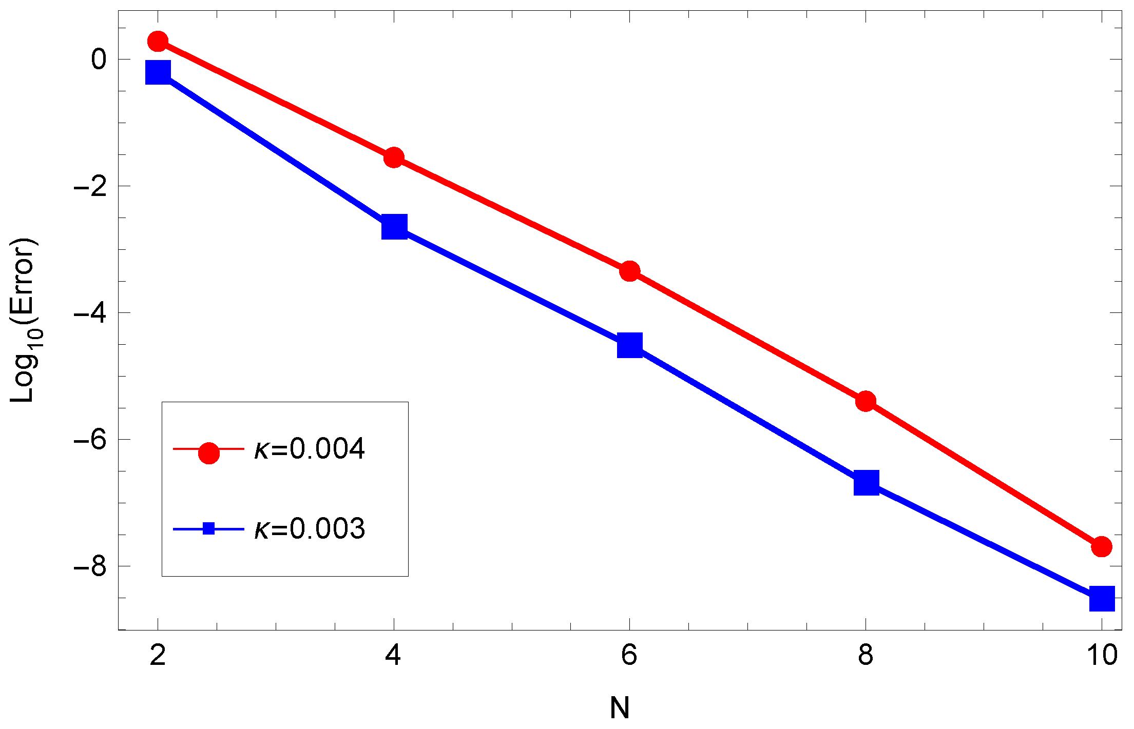
  • The trunction error estimate is dominated by the following estimate | U U K | = O ( 4 K ) .
Proof. 
Following similar procedures to those followed in Abd-Elhameed et al. in [21] along with Theorems 6 and 7, we get the desired result.  □

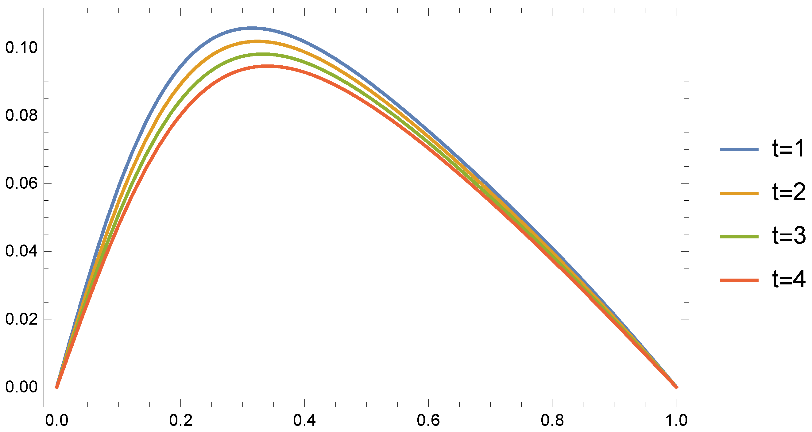
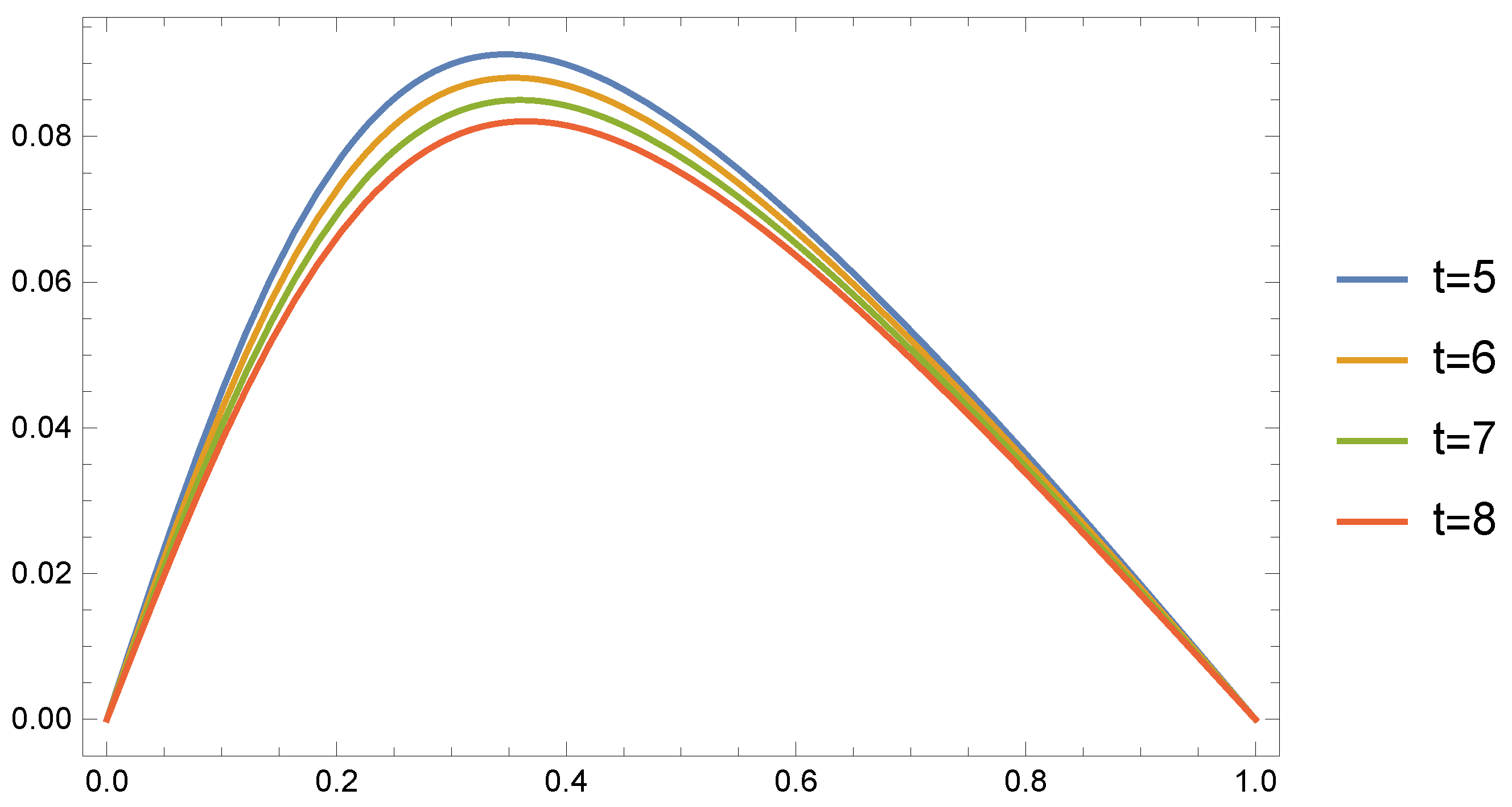
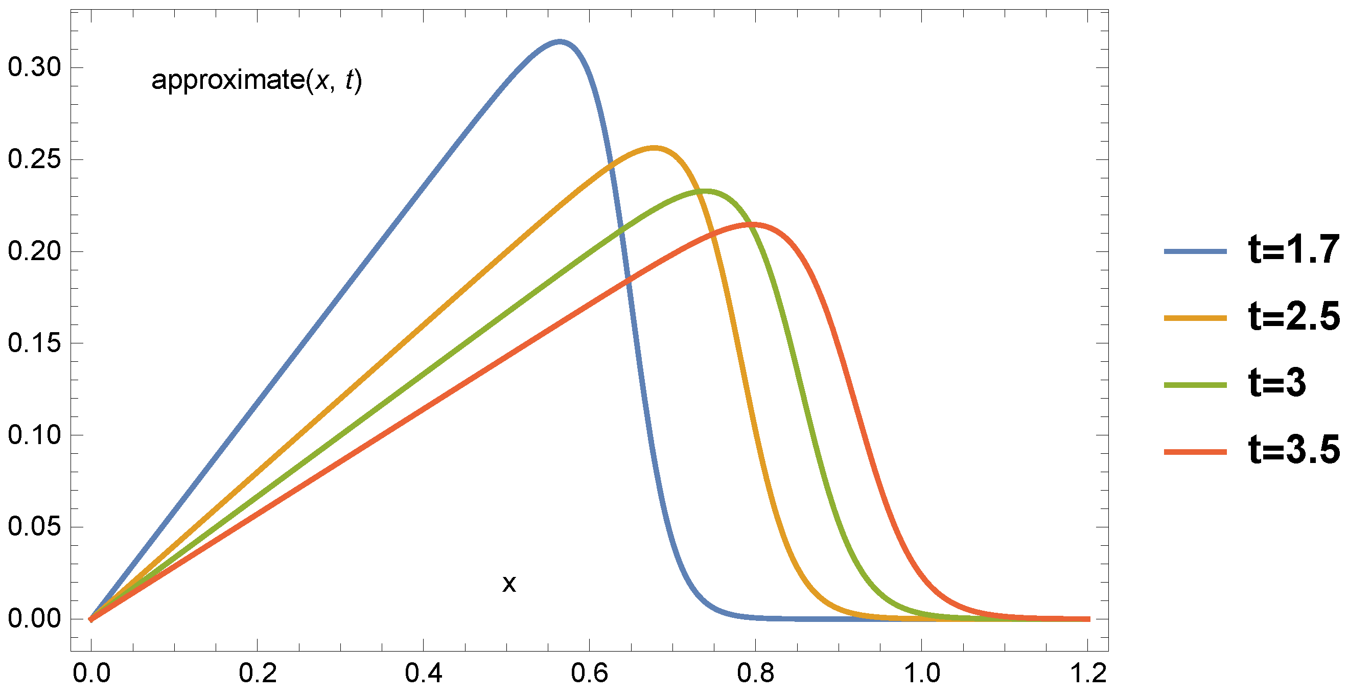
6. Numerical Experiments and Comparisons

This section is confined to displaying some numerical examples to show the applicability and efficiency of our shifted Chebyshev sixth kind tau method (SC6TM). Furthermore, comparisons with some other methods in the literature are presented.
Example 1
([41]). Consider the following non-linear Burgers’ equation
U t + U U x = ν 2 U x 2 , ( x , t ) Ω = ( 0 , 1 ) × ( 0 , τ ) ,
governed by the initial condition:
U ( x , 0 ) = sin ( π x ) , x ( 0 , 1 ) ,
and by the homogeneous boundary conditions:
U ( 0 , t ) = U ( 1 , t ) = 0 , t ( 0 , τ ) .
The analytic solution of (64)–(66) can be obtained with the aid of Hopf–Cole method ([50]). This solution is obtained in [41]. It is given by
U ( x , t ) = 2 π ν k = 1 a k e k 2 π 2 ν t sin ( k π x ) a 0 + k = 1 a k e k 2 π 2 ν t cos ( k π x ) ,
with the following Fourier coefficients
a 0 = 0 1 exp { ( 2 π ν ) 1 ( 1 cos ( π x ) ) } d x , a k = 2 0 1 exp { ( 2 π ν ) 1 ( 1 cos ( π x ) ) } cos ( k π x ) d x , k > 1 .
In Table 1, we report a comparison between the exact solution, our proposed method and Chebyshev wavelets Picard method (CWPM) that developed in [41] for solving Example 1, while in Figure 1 and Figure 2, we illustrate the behavior of the resulting approximate solutions for different values of t and for N = 5 .
Example 2
([41]). Consider Equation (64) governed by the same boundary conditions (66) but with the following initial condition:
U ( x , 0 ) = sin ( 2 π x ) , x ( 0 , 1 ) ,
In this case, the Fourier coefficients are given by
a 0 = 0 1 exp { ( 4 π ν ) 1 ( 1 cos ( 2 π x ) ) } d x , a k = 2 0 1 exp { ( 4 π ν ) 1 ( 1 cos ( 2 π x ) ) } cos ( k π x ) d x , k > 1 .
In Table 2, we report the errors resulted from the application of SC6TM for Example 2, while in Figure 3 and Figure 4, we illustrate the behavior of the resulting approximate solutions for different values of t when N = 6 .
Example 3
([41]). We consider Equation (64) governed by the same boundary conditions (66) but subject to the initial condition:
U ( x , 0 ) = 4 x ( 1 x ) , x ( 0 , 1 ) .
In this case the Fourier coefficients are given by
a 0 = 0 1 exp { ( 3 ν ) 1 ( 3 x 2 2 x 3 ) } d x , a k = 2 0 1 exp { ( 3 ν ) 1 ( 3 x 2 2 x 3 ) } cos ( k π x ) d x , k > 1 .
In Figure 5 and Figure 6, the behavior of the approximate solutions resulted from the application of SC6TM for different values of t and for N = 10 is illustrated. Furthermore, in Figure 7, we illustrate the Log-error plot for different values of N.
Example 4
([45,47]). Consider Equation (64) subject to the initial condition:
U ( x , 1 ) = x e 1 8 ν e x 2 4 ν + 1 , x ( 0 , 1.2 ) ,
and the boundary conditions:
U ( 0 , t ) = U ( 1.2 , t ) = 0 ,
in this case the exact solution for this problem for t > 1 is given by
U ( x , t ) = x t e 1 8 ν t e x 2 4 ν t + 1 .
We apply our proposed algorithm for the case corresponding to ν = 0.005 , N = 10 , and T = 3.6 . In Table 3, we report a comparison between the maximum absolute errors of Example 4 resulted from the application of our proposed method, the method developed in [45], and the three methods in [47]. In addition, Figure 8 displays the approximate solutions of Example 4 for different values of t, while Figure 9 illustrates the behavior of the errors resulted form the application of our proposed method for different values of t.

7. Conclusions

In this work, we developed new expressions for the high-order derivatives of Chebyshev polynomials of the sixth kind in terms of their original ones. We proved that these derivatives can be expressed in terms of certain terminating hypergeometric functions of unit argument that can be summed in some specific cases. These expressions along with some other formulas concerned with the sixth kind Chebyshev polynomials are employed to solve the one dimensional Burgers’ differential equation via the application of the spectral tau method. The proposed method transforms the non-linear Burgers’ equation governed by its initial and boundary conditions into a non-linear algebraic system that can be solved through any suitable numerical solver. The presented numerical examples show that our proposed algorithm is applicable and efficient. We do believe that our derived theoretical formulas are new and useful. Furthermore, they can be utilized to solve several types of linear and non-linear differential equations. In addition, it is worthy to point out here that the investigation of the generalized ultraspherical polynomials theoretically and practically needs extensive work, and we plan to investigate them as future work.

Funding

The author received no funding for this study.

Institutional Review Board Statement

Not applicable.

Informed Consent Statement

Not applicable.

Data Availability Statement

Not applicable.

Acknowledgments

The author would like to thank the editor and the reviewers for carefully reading the article and also for their constructive and valuable comments which have improved the paper in its present form.

Conflicts of Interest

The author declares no conflict of interest.

References

  1. Kim, T.; Kim, D.S.; Lee, H.; Kwon, J. studies in sums of finite products of the second, third, and fourth kind Chebyshev polynomials. Mathematics 2020, 8, 210. [Google Scholar] [CrossRef] [Green Version]
  2. Leong, Y.; Cheab, S.; Soeung, S.; Wong, P.W. A new class of dual-band waveguide filters based on Chebyshev polynomials of the second kind. IEEE Access 2020, 8, 28571–28583. [Google Scholar] [CrossRef]
  3. Oloniiju, S.D.; Goqo, S.P.; Sibanda, P. A Chebyshev pseudo-spectral method for the multi-dimensional fractional Rayleigh problem for a generalized Maxwell fluid with Robin boundary conditions. Appl. Numer. Math. 2020, 152, 253–266. [Google Scholar] [CrossRef]
  4. Lashenov, K.V. On a class of orthogonal polynomials. Sci. Notes Leningr. Gov. Pedagog. Inst. 1953, 89, 167–189. [Google Scholar]
  5. Masjed-Jamei, M. Some New Classes of Orthogonal Polynomials and Special Functions: A Symmetric Generalization of Sturm-Liouville Problems and its Consequences. Ph.D. Thesis, Department of Mathematics, University of Kassel, Kassel, Germany, 2006. [Google Scholar]
  6. Abd-Elhameed, W.M.; Youssri, Y.H. Fifth-kind orthonormal Chebyshev polynomial solutions for fractional differential equations. Comput. Appl. Math. 2018, 37, 2897–2921. [Google Scholar] [CrossRef]
  7. Abd-Elhameed, W.M.; Youssri, Y.H. Sixth-Kind Chebyshev spectral approach for solving fractional differential equations. Int. J. Nonlinear Sci. Numer. Simul. 2019, 20, 191–203. [Google Scholar] [CrossRef]
  8. Abd-Elhameed, W.M.; Youssri, Y.H. Neoteric formulas of the monic orthogonal Chebyshev polynomials of the sixth-kind involving moments and linearization formulas. Adv. Differ. Equ. 2021, 2021, 84. [Google Scholar] [CrossRef]
  9. Jafari, H.; Babaei, A.; Banihashemi, S. A novel approach for solving an inverse reaction–diffusion–convection problem. J. Optim. Theory Appl. 2019, 183, 688–704. [Google Scholar] [CrossRef]
  10. Pandey, P.; Gómez-Aguilar, J.F. On solution of a class of nonlinear variable order fractional reaction–diffusion equation with Mittag–Leffler kernel. Numer. Methods Partial Differ. Equ. 2021, 37, 998–1011. [Google Scholar] [CrossRef]
  11. Öztürk, Y. solution for the system of Lane–Emden type equations using Chebyshev polynomials. Mathematics 2018, 6, 181. [Google Scholar] [CrossRef] [Green Version]
  12. Hassani, H.; Machado, J.A.T.; Avazzadeh, Z.; Naraghirad, E. Generalized shifted Chebyshev polynomials: Solving a general class of nonlinear variable order fractional PDE. Commun. Nonlinear Sci. Numer. Simul. 2020, 85, 105229. [Google Scholar] [CrossRef]
  13. Habenom, H.; Suthar, D.L. Numerical solution for the time-fractional Fokker–Planck equation via shifted Chebyshev polynomials of the fourth kind. Adv. Differ. Equ. 2020, 2020, 315. [Google Scholar] [CrossRef]
  14. Duangpan, A.; Boonklurb, R.; Treeyaprasert, T. finite integration method with shifted Chebyshev polynomials for solving time-fractional Burgers’ equations. Mathematics 2019, 7, 1201. [Google Scholar] [CrossRef] [Green Version]
  15. Canuto, C.; Hussaini, M.; Quarteroni, A.; Zang, T.A. Spectral Methods in Fluid Dynamics; Springer: Berlin, Germany, 1988. [Google Scholar]
  16. Shizgal, B. Spectral Methods in Chemistry and Physics; Springer: Dordrecht, The Netherlands, 2015. [Google Scholar]
  17. Hesthaven, J.; Gottlieb, S.; Gottlieb, D. Spectral Methods for Time-Dependent Problems; Cambridge University Press: Cambridge, UK, 2007; Volume 21. [Google Scholar]
  18. Doha, E.H.; Abd-Elhameed, W.M. On the coefficients of integrated expansions and integrals of Chebyshev polynomials of third and fourth kinds. Bull. Malays. Math. Sci. Soc. 2014, 37, 383–398. [Google Scholar]
  19. Doha, E.H.; Abd-Elhameed, W.M.; Youssri, Y.H. Efficient spectral-Petrov–Galerkin methods for the integrated forms of third-and fifth-order elliptic differential equations using general parameters generalized Jacobi polynomials. Appl. Math. Comput. 2012, 218, 7727–7740. [Google Scholar] [CrossRef]
  20. Youssri, Y.H.; Abd-Elhameed, W.M. Numerical spectral Legendre-Galerkin algorithm for solving time fractional telegraph equation. Rom. J. Phys. 2018, 63, 1–16. [Google Scholar]
  21. Abd-Elhameed, W.M.; Doha, E.H.; Youssri, Y.H.; Bassuony, M.A. New Tchebyshev-Galerkin operational matrix method for solving linear and nonlinear hyperbolic telegraph type equations. Numer. Methods Partial Differ. Equ. 2016, 32, 1553–1571. [Google Scholar] [CrossRef]
  22. Faghih, A.; Mokhtary, P. An efficient formulation of Chebyshev tau method for constant coefficients systems of multi-order FDEs. J. Sci. Comput. 2020, 82, 6. [Google Scholar] [CrossRef]
  23. Mohammadi, F.; Cattani, C. A generalized fractional-order Legendre wavelet Tau method for solving fractional differential equations. J. Comput. Appl. Math. 2018, 339, 306–316. [Google Scholar] [CrossRef]
  24. Doha, E.H.; Abd-Elhameed, W.M. Accurate spectral solutions for the parabolic and elliptic partial differential equations by the ultraspherical tau method. J. Comput. Appl. Math. 2005, 181, 24–45. [Google Scholar] [CrossRef] [Green Version]
  25. Abd-Elhameed, W.M.; Youssri, Y.H. Spectral tau algorithm for certain coupled system of fractional differential equations via generalized Fibonacci polynomial sequence. Iran. J. Sci. Technol. Trans. A Sci. 2019, 43, 543–554. [Google Scholar] [CrossRef]
  26. Abd-Elhameed, W.M.; Machado, J.A.T.; Youssri, Y.H. Hypergeometric fractional derivatives formula of shifted Chebyshev polynomials: Tau algorithm for a type of fractional delay differential equations. Int. J. Nonlinear Sci. Numer. Simul. 2021. [Google Scholar] [CrossRef]
  27. Khader, M.M.; Adel, M. Numerical approach for solving the Riccati and logistic equations via QLM-rational Legendre collocation method. Comput. Appl. Math. 2020, 39, 166. [Google Scholar] [CrossRef]
  28. Costabile, F.; Napoli, A. Collocation for high order differential equations with two-points Hermite boundary conditions. Appl. Numer. Math. 2015, 87, 157–167. [Google Scholar] [CrossRef]
  29. Costabile, F.; Napoli, A. A method for high-order multipoint boundary value problems with Birkhoff-type conditions. Intern. J. Comput. Math. 2015, 92, 192–200. [Google Scholar] [CrossRef]
  30. Saw, V.; Kumar, S. The Chebyshev collocation method for a class of time fractional convection-diffusion equation with variable coefficients. Math. Methods Appl. Sci. 2021, 44, 6666–6678. [Google Scholar] [CrossRef]
  31. Abd-Elhameed, W.M. On solving linear and nonlinear sixth-order two point boundary value problems via an elegant harmonic numbers operational matrix of derivatives. CMES Comput. Model. Eng. Sci. 2014, 101, 159–185. [Google Scholar]
  32. Napoli, A.; Abd-Elhameed, W.M. An innovative harmonic numbers operational matrix method for solving initial value problems. Calcolo 2017, 54, 57–76. [Google Scholar] [CrossRef]
  33. Abd-Elhameed, W.M. New product and linearization formulae of Jacobi polynomials of certain parameters. Integral Transform. Spec. Funct. 2015, 26, 586–599. [Google Scholar] [CrossRef]
  34. Abd-Elhameed, W.M. New formulae between Jacobi polynomials and some fractional Jacobi functions generalizing some connection formulae. Anal. Math. Phys. 2019, 9, 73–98. [Google Scholar] [CrossRef]
  35. Abd-Elhameed, W.M.; Ali, A. New specific and general linearization formulas of some classes of Jacobi polynomials. Mathematics 2021, 9, 74. [Google Scholar] [CrossRef]
  36. Abd-Elhameed, W.M.; Youssri, Y.H. New formulas of the high-order derivatives of fifth-kind Chebyshev polynomials: Spectral solution of the convection–diffusion equation. Numer. Methods Partial Differ. Equ. 2021. [Google Scholar] [CrossRef]
  37. Doha, E.H.; Abd-Elhameed, W.M.; Bassuony, M.A. On the coefficients of differentiated expansions and derivatives of Chebyshev polynomials of the third and fourth kinds. Acta Math. Sci. 2015, 35, 326–338. [Google Scholar] [CrossRef]
  38. Srivastava, H.M. Some Clebsch-Gordan type linearisation relations and other polynomial expansions associated with a class of generalised multiple hypergeometric series arising in physical and quantum chemical applications. J. Phys. A Math. Gen. 1988, 21, 4463. [Google Scholar] [CrossRef]
  39. Srivastava, H.M. A unified theory of polynomial expansions and their applications involving Clebsch-Gordan type linearization relations and Neumann series. Astrophys. Space Sci. 1988, 150, 251–266. [Google Scholar] [CrossRef]
  40. Srivastava, H.M.; Niukkanen, A.W. Some Clebsch-Gordan type linearization relations and associated families of Dirichlet integrals. Math. Comput. Model. 2003, 37, 245–250. [Google Scholar] [CrossRef]
  41. Hariharan, G.; Swaminathan, G.; Sripathy, B. An efficient operational matrix approach for the solutions of Burgers’ and fractional Burgers’ equations using wavelets. J. Math. Chem. 2021, 59, 554–573. [Google Scholar] [CrossRef]
  42. Singh, B.K.; Gupta, M. A new efficient fourth order collocation scheme for solving Burgers’ equation. Appl. Math. Comput. 2021, 399, 126011. [Google Scholar]
  43. Xie, S.S.; Heo, S.; Kim, S.; Woo, G.; Yi, S. Numerical solution of one-dimensional Burgers’ equation using reproducing kernel function. J. Comput. Appl. Math. 2008, 214, 417–434. [Google Scholar] [CrossRef] [Green Version]
  44. Bratsos, A.G. A fourth-order numerical scheme for solving the modified Burgers equation. Comput. Math. Appl. 2010, 60, 1393–1400. [Google Scholar] [CrossRef] [Green Version]
  45. Arora, G.; Singh, B.K. Numerical solution of Burgers’ equation with modified cubic B-spline differential quadrature method. Appl. Math. Comput. 2013, 224, 166–177. [Google Scholar] [CrossRef]
  46. Mittal, R.C.; Jain, R.K. Numerical solutions of nonlinear Burgers’ equation with modified cubic B-splines collocation method. Appl. Math. Comput. 2012, 218, 7839–7855. [Google Scholar] [CrossRef]
  47. Korkmaz, A.; Dağ, İ. Cubic B-spline differential quadrature methods and stability for Burgers’ equation. Eng. Comput. 2013, 30, 320–344. [Google Scholar] [CrossRef]
  48. Kukreja, V.K. An improvised collocation algorithm with specific end conditions for solving modified Burgers equation. Numer. Methods Partial Differ. Equ. 2021, 37, 874–896. [Google Scholar]
  49. Yang, X.J.; Gao, F.; Srivastava, H.M. Exact travelling wave solutions for the local fractional two-dimensional Burgers-type equations. Comput. Math. Appl. 2017, 73, 203–210. [Google Scholar] [CrossRef]
  50. Cole, J.D. On a quasi-linear parabolic equation occurring in aerodynamics. Q. Appl. Math. 1951, 9, 225–236. [Google Scholar] [CrossRef] [Green Version]
Figure 1. The approximate solutions of Example 1 at different times.
Fractalfract 05 00053 g001
Figure 2. The approximate solutions of Example 1 at different times.
Fractalfract 05 00053 g002
Figure 3. The approximate solutions of Example 2 at different times.
Fractalfract 05 00053 g003
Figure 4. The approximate solutions of Example 2 at different times.
Fractalfract 05 00053 g004
Figure 5. The approximate solutions of Example 3 at different times.
Fractalfract 05 00053 g005
Figure 6. The approximate solutions of Example 3 at different times.
Fractalfract 05 00053 g006
Figure 7. Log-errors of Example 3 for different values of ν and N.
Fractalfract 05 00053 g007
Figure 8. The approximate solutions of Example 4 for different values of t.
Fractalfract 05 00053 g008
Figure 9. Errors of Example 4 for different values of t.
Fractalfract 05 00053 g009
Table 1. Comparison between the exact solution, CWPM solution and SC6TM solution of Example 1.
x = 0.25 x = 0.5 x = 0.75
tSC6TMCWPM [41]ExactSC6TMCWPM [41]ExactSC6TMCWPM [41]Exact
0.10.261480.261470.261480.383420.38340.383420.281570.281560.28157
0.150.161480.161460.161480.234060.234040.234060.169740.169730.16974
0.20.099470.099460.099470.142890.142880.142890.102660.102650.10266
0.250.061080.061070.061080.087230.087210.087230.062290.062290.06229
Table 2. Errors of Example 2, when ν = 1 and N = 6 .
x0.10.20.30.40.50.60.70.80.9
t = 0.2 1.2 × 10 6 2.4 × 10 6 3.4 × 10 6 5.7 × 10 6 5.2 × 10 6 6.1 × 10 6 6.7 × 10 6 8.1 × 10 6 1.9 × 10 5
t = 0.4 1.2 × 10 6 3.2 × 10 6 5.4 × 10 6 6.3 × 10 6 8.2 × 10 6 7.2 × 10 6 7.8 × 10 6 8.3 × 10 6 1.4 × 10 5
t = 0.6 1.2 × 10 6 3.2 × 10 6 3.6 × 10 6 5.4 × 10 6 5.5 × 10 6 5.5 × 10 6 6.8 × 10 6 7.1 × 10 6 1.9 × 10 5
t = 0.8 3.2 × 10 6 4.2 × 10 6 7.4 × 10 5 6.8 × 10 5 7.3 × 10 5 4.4 × 10 5 7.6 × 10 5 8.6 × 10 5 2.2 × 10 5
Table 3. Comparison between different errors of Example 4, when t = 3.6 .
Method [45] [47]-I [47]-II [47]-III SC6TM
L E r r o r 7.0 × 10 5 4.6 × 10 4 5.2 × 10 4 5.4 × 10 4 2.2 × 10 6
Publisher’s Note: MDPI stays neutral with regard to jurisdictional claims in published maps and institutional affiliations.

