1. Introduction
Droplet dispensing is the process of ejecting discrete fluidic volumes with two immiscible fluids [
1]. The ejection process can happen in various droplet breakup regimes, one of them being an on-demand breakup. The dispense is performed by providing the fluid with enough energy as a short actuation pulse in the form of thermal fluctuations or mechanical vibrations to overcome energies holding the fluid back, such as capillary forces.
When this actuation pulse is applied, the droplet takes a teat shape due to the positive pressure and the opposing surface tension where the fluid touches the orifice [
2]. Next, a tail is formed, caused by the inertia of the liquid, and this tail is broken by the upward pull of the negative pressure created. After leaving the nozzle, the droplet continuously changes its shape from the initial cylindrical-like shape to wobbling between tear-like and spherical shapes, until it becomes stably spherical due to the surface tension of the fluid. Hence, during the initial phase of the ejection, the droplet undergoes a shape evolution before reaching a stable spherical state, i.e., it follows a specific spatiotemporal trajectory. For non-contact dispensers (such as PipeJet P9, BioFluidix GmbH, Freiburg im Breisgau, Germany [
3]), this spatiotemporal motion pattern depends on various factors: the geometries involved (such as the characteristic length (D) of the dispenser), the actuation dynamics (such as the stroke length (SL) and downstroke velocity (DV)), the rheological (such as viscosity) and physical properties (such as density) of the liquid being dispensed, the surface effects, and the environmental variables (such as temperature and relative humidity). This primary droplet can also be followed by secondary droplets known as satellites.
To simplify the modeling of the ejection events, characteristic numbers can be used. These numbers are dimensionless quantities and hence systems with the same characteristic numbers behave similarly regardless of factors such as their scale. The dimensionless numbers which are interesting for the droplet ejection process are the Weber number (
We) and the Ohnesorge number (
Oh) [
1]. The droplets will follow different spatiotemporal trajectories when ejected either with a different
We and/or with a different
Oh.
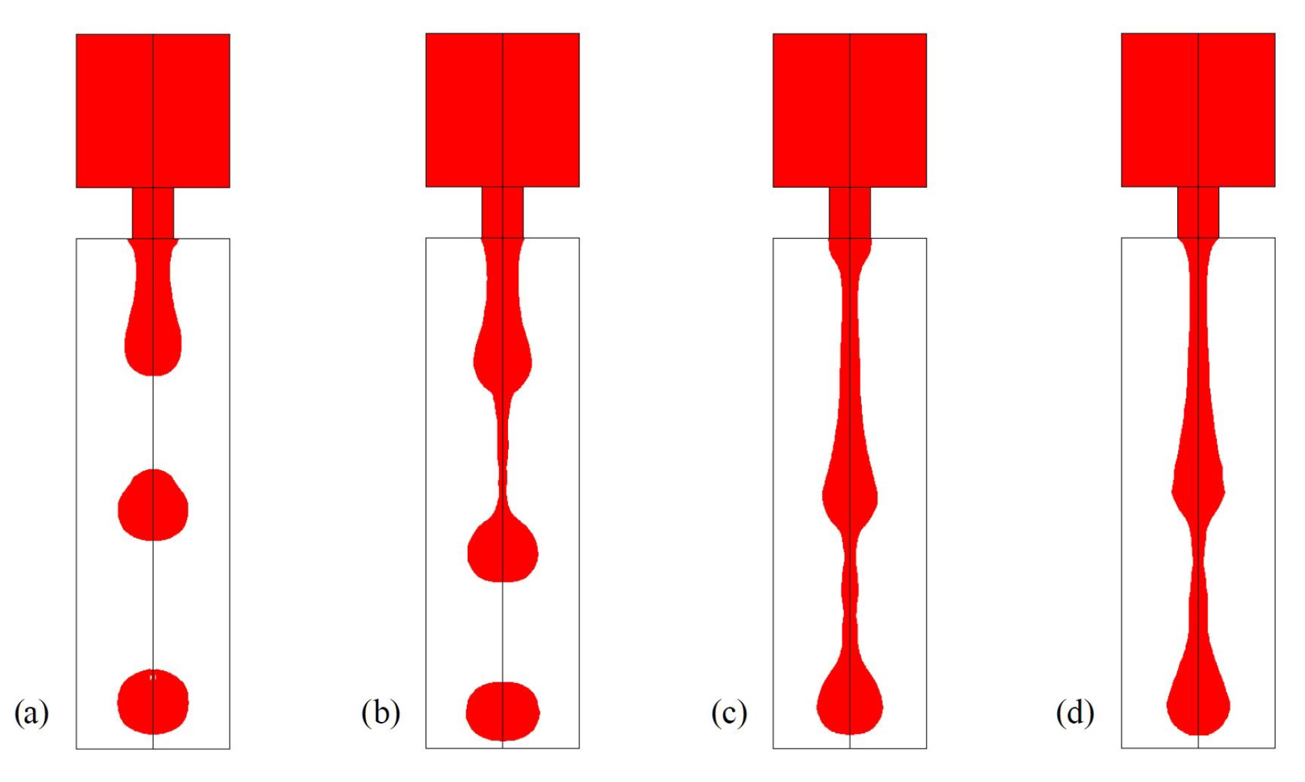
Figure 1 shows the output of a simulation conducted wherein fluid is ejected at various
Oh [
4].
We is the ratio between the kinetic energy of a fluid and its surface energy [
1]. Therefore, it depends on the actuation parameters and the liquid properties, whereas
Oh relates the following: internal viscous dissipation to inertia and surface tension. Therefore, it depends on the liquid properties and the characteristic length. The relation between
We,
Oh, and the Reynolds number (
Re) is given in Equation (
1)
where
is the dynamic viscosity of the liquid,
is the density,
D is the characteristic length, and
is the surface tension. The spatiotemporal trajectories formed by the ejected droplets can be imaged using a high-speed camera.
Even though mathematical models exist to create these droplet trajectories from the initial conditions [
5], solving the inverse problem (i.e., estimating the initial conditions from the trajectories) is not trivial. Nonetheless, such a solver is useful in practical scenarios. It could be used, for instance, to adjust dispenser parameters on the fly as the liquid properties change due to temperature fluctuations. As neural networks are universal approximators [
6], these can be applied to solve the aforementioned problem. Convolutional neural networks (CNNs) are great tools for capturing the spatial and spatiotemporal content [
7]. Hence, these can be used to identify liquids with different
Oh from the captured images and image sequences (videos) of the dispensed droplets.
Convolutional neural networks (CNNs), which belong to the class of machine learning algorithms known as deep learning (DL) [
8], build complex representations by taking simpler representations as input in an end-to-end manner. This ability to automatically build new constructs on top of existing representations gives DL the ability to extract the non-obvious complex representations from the underlying data. This can then be used to perform tasks such as distinguishing between different classes present in the data, i.e., classification. The training for this classification process can be conducted in a supervised fashion if the type of liquid in the image, i.e., the label, is known.
As droplets with different Oh follow different spatiotemporal trajectories, they may form unique shapes. This indicates that neural networks with only 2D extractors may be enough and 3D information processing may not be needed. To test this, different CNN architectures with pure 2D convolutions, pure 3D convolutions, or 3D–2D mixed convolutions were compared.
2. Data Acquisition
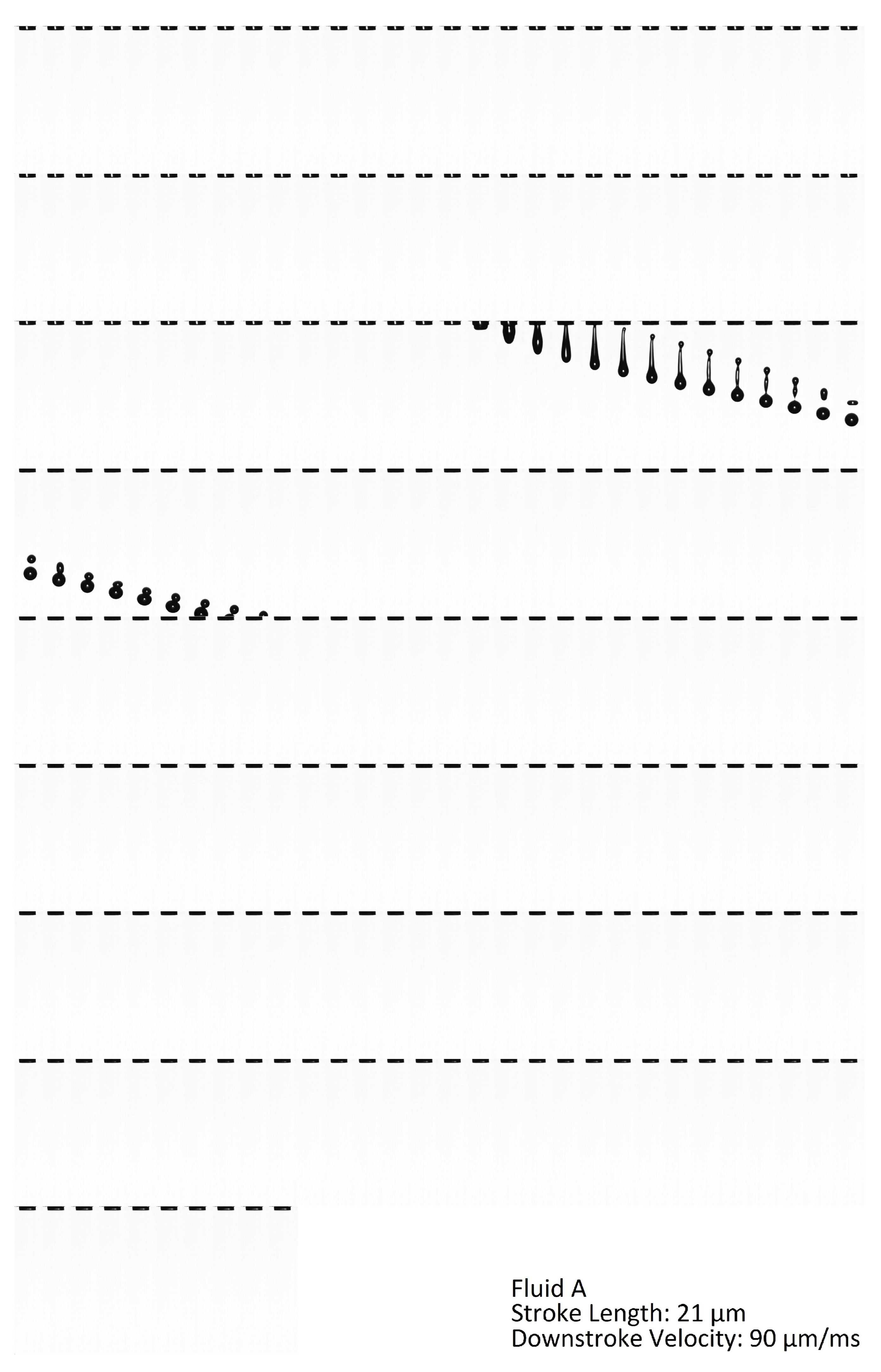
Data acquisition is one of the major tasks in the DL pipeline. To fulfill the need of acquiring a large amount of labeled data, an automated data acquisition setup, named TestRig, was used. For each droplet dispense, a sequence of 250 frames at 6806 frames per second was recorded.
Figure A2 shows an example sequence. During the data acquisition process, various sources for shortcut learning [
9] such as poor lighting, poor focus, tilting of the dispenser nozzle, etc., were avoided. The following topics are discussed in the following subchapters: hardware and software of the TestRig (
Section 2.1), the test liquids used (
Section 2.2), as well as hardware configuration and acquisition protocols (
Section 2.3).
2.1. Hardware and Software of the TestRig
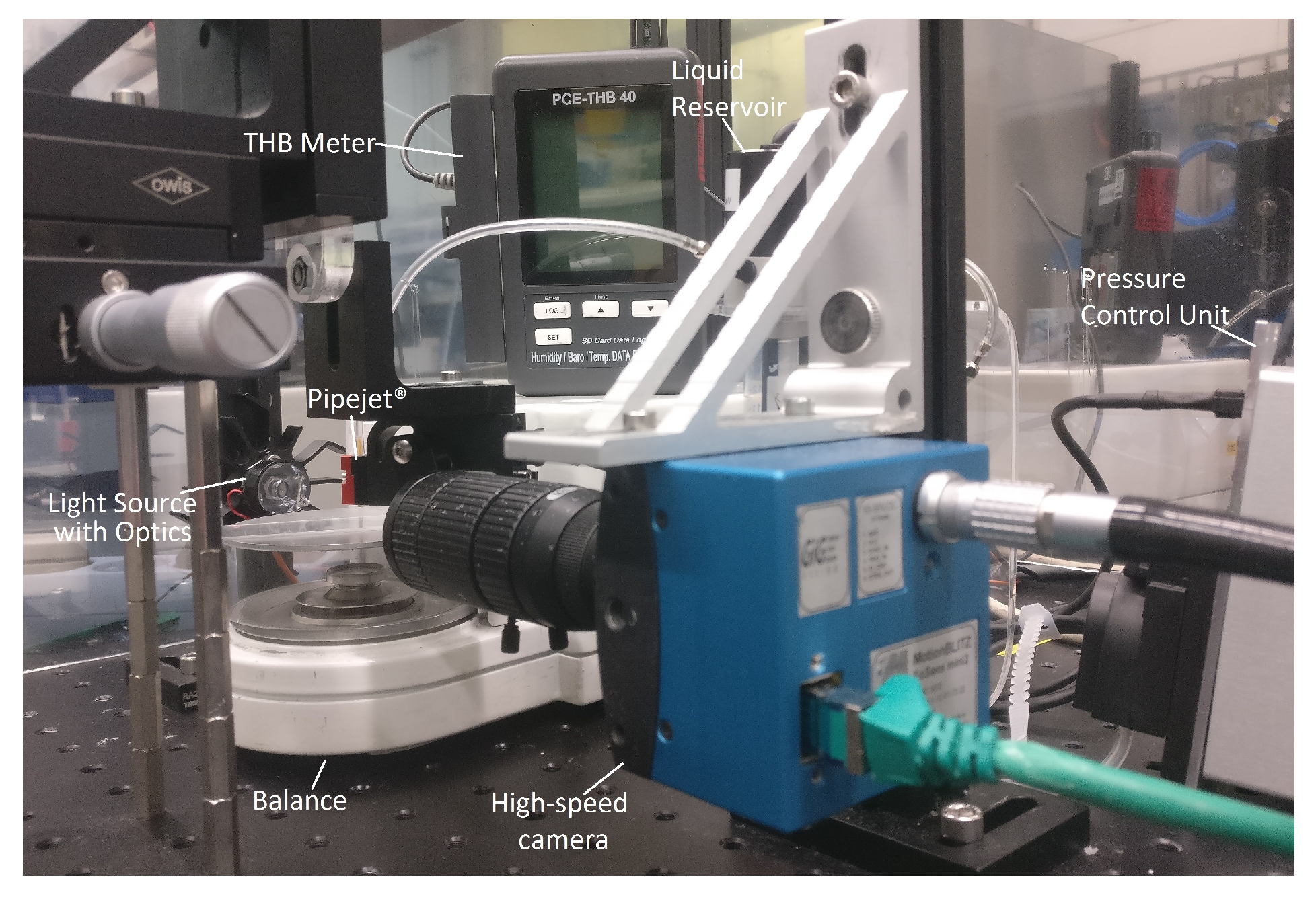
Figure 2 shows the TestRig. It was built on top of an optical breadboard. The droplets were dispensed using a nanoliter non-contact droplet dispenser (BioFluidix PipeJet
®, Freiburg im Breisgau, Germany [
3]) mounted on a three-axis precision stage. The nozzles had an inner diameter of 500
. The falling droplets were imaged as shadows by positioning the dispenser nozzle between a light-emitting diode and a high-speed camera (MotionBLITZ EoSens
® mini2, Mikrotron GmbH, Unterschleissheim, Germany). To reduce the influence of convection on the trajectory of the droplets, the setup was covered with walls and a lid.
The liquid pressure was regulated during the acquisition using a pressure control module (ActivePCR, BioFluidix GmbH, Freiburg im Breisgau, Germany). Additionally, the weight of the falling droplets was measured using a micro-weighing balance (SC2 Ultra-Microbalance, Sartorius AG, Goettingen, Germany) placed under the orifice, and the ambient temperature, pressure, and humidity were logged with a thermo-hygrometer.
The TestRig was controlled via an in-house developed software called ♯Drop [
10]. It was used to trigger the camera, configure the parameters of the PipeJet
® actuation, and log mass, ambient temperature, relative humidity, and pressure readings. Next, MotionBLITZ
® Director2 was used to configure and operate the camera. Furthermore, Biofluidix Pipejet
® Control software was used to configure and operate the pressure control unit.
2.2. Used Liquids
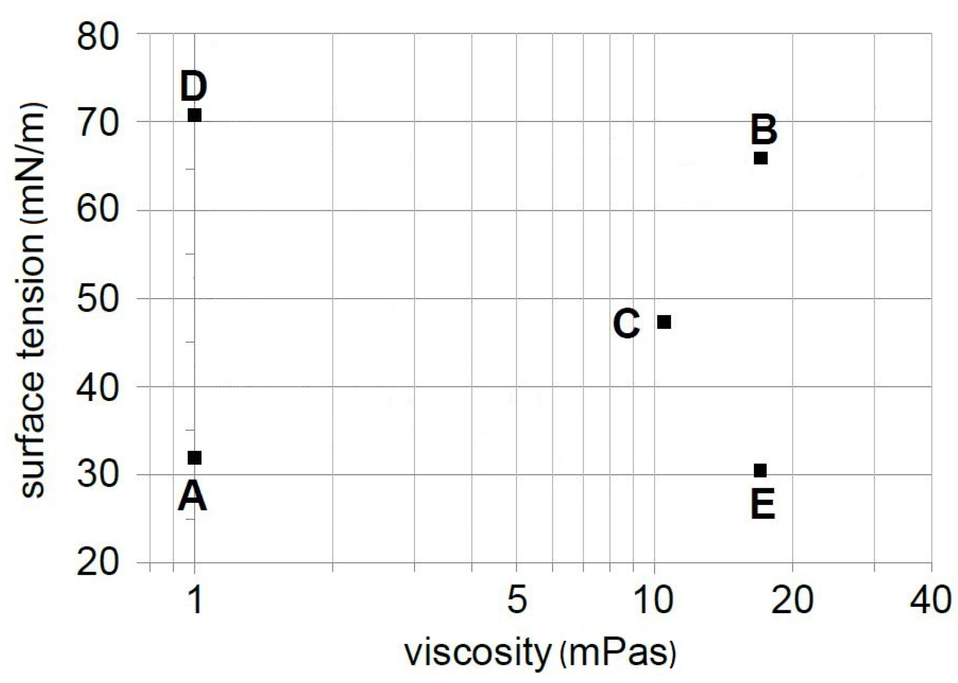
This study uses five of the eight model liquids developed in [
11], covering the whole range of viscosity and surface tension of 646 of the most common in vitro diagnostics reagents.
Figure 3 presents the surface tension vs. viscosity for the model liquids.
Table 1 summarizes fluid properties, the
Oh for a 500
nozzle, and the components shortlisted from [
11]. There were little fluctuations in the ambient temperatures (23.2 °C to 28.6 °C) during acquisition, but the resulting error in the
Oh calculation (for water) was not significant (0.54 × 10
−3) as all the other liquids used in this study have significantly larger
Oh.
2.3. Hardware Parameters and Acquisition Protocol
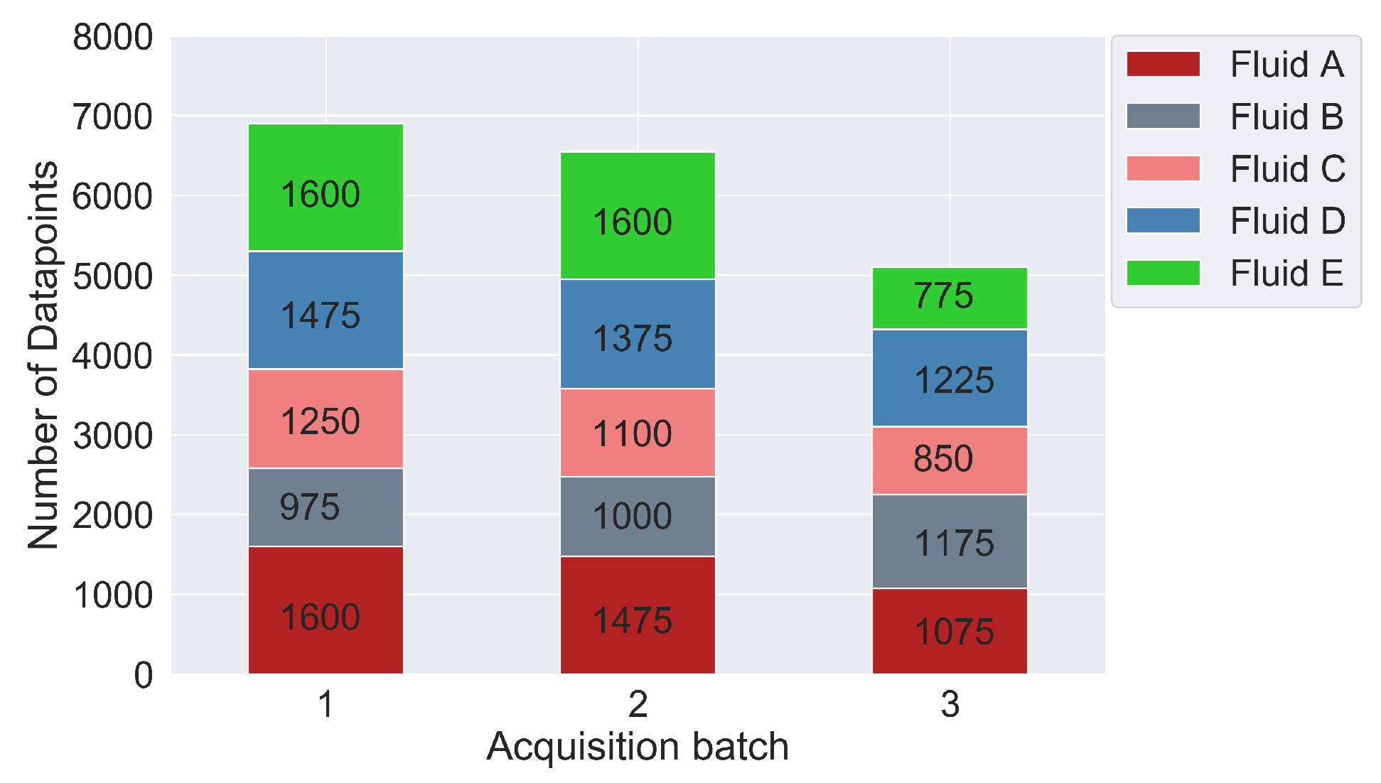
A set of 64 configurations was chosen for driving the Pipejet®. Each of these configurations was repeated 25 times consecutively, leading to a total of 1600 dispenses. Each configuration was a combination of one of the eight SLs (10, 12, 14, 16, 18, 21, 23, or 25 ) and one of the eight DVs (60, 70, 80, 90, 100, 110, 120, or 130 /) with all the DVs sequenced in ascending order with a single SL before moving to a higher SL. An acquisition batch is a set containing one acquisition cycle from all five test liquids. The data acquisition was conducted in three acquisition batches.
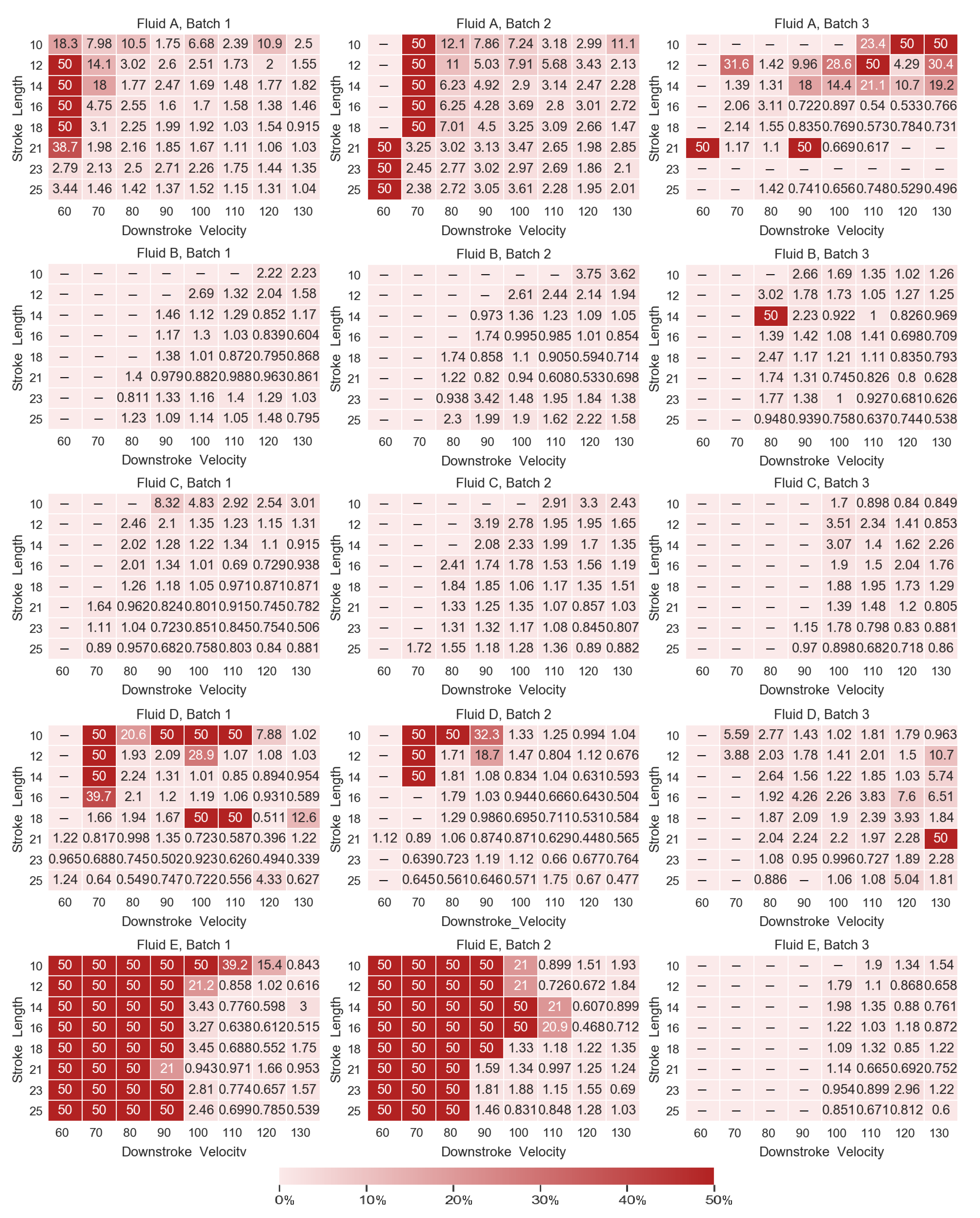
Depending on the viscosity of the individual liquids, some actuation configurations did not provide enough energy to eject the liquid. These invalid configurations were filtered out of the dataset. This resulted in 31 to 64 valid configurations based on the liquid, nozzle condition, and environmental conditions.
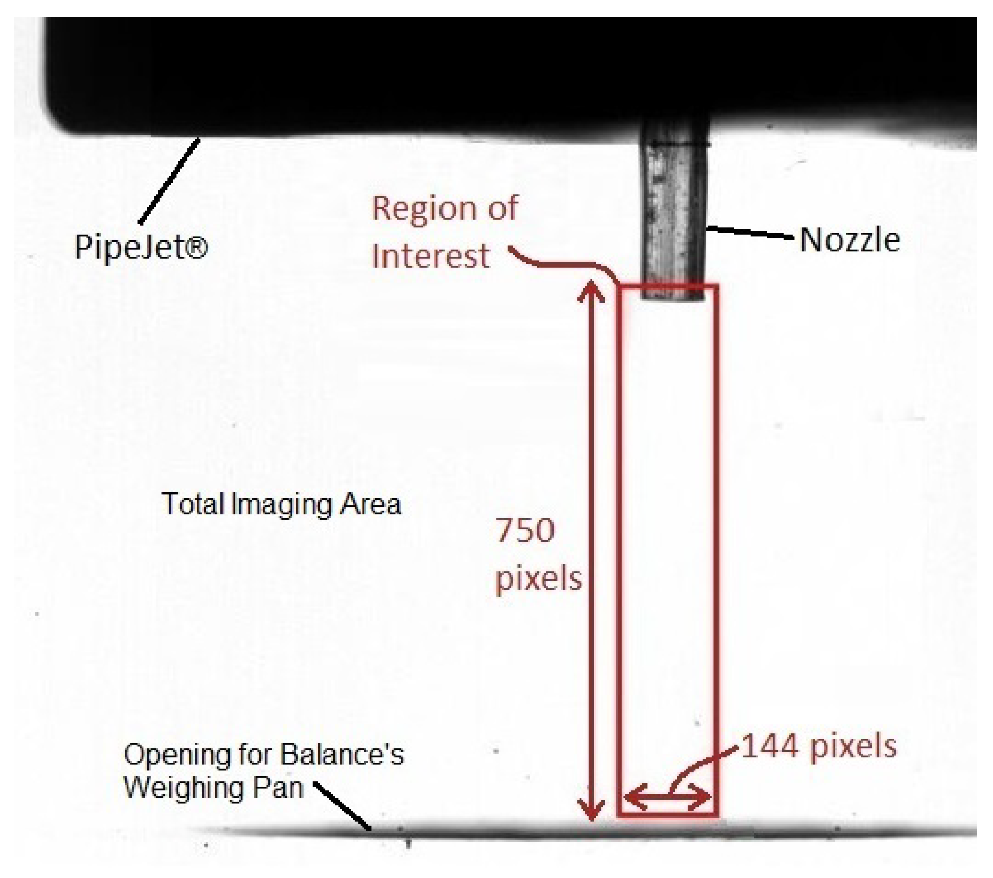
The camera was configured by defining a frame size with a height of 750 pixels and a width of 144 pixels. The height was experimentally determined to ensure that, even for the drop with the longest tail (produced with the liquid with the highest Oh, liquid E), there should exist at least one frame that contains the entire droplet, from head to tail. Next, the width was obtained by observing the number of pixels covered by the nozzle and multiplying it by 3 to account for the tilting of the nozzle. The configurations resulted in a maximum frame rate of 6806 fps for the current hardware. For each dispense, 250 images were acquired at this frame rate.
The tip of the nozzle was kept in the frame. This was primarily because the droplets have a high degree of spatiotemporal changes when leaving the nozzle, which can be interesting for the classification task. Moreover, the nozzle of known diameter can also be used as a reference object for camera zoom and focus. A shadowgraph of the field of view in the imaging plane is given in
Figure 4.
The time difference between two consecutive dispenses was 31 s for the first two acquisition batches to save all the acquired images. It was increased to 33 s in the third acquisition batch to give the dataset a bit of diversity and improve the generalization of the trained model on new, unseen datasets. Gravimetric weight analysis was performed according to the GRM method [
12,
13] with settling and measuring times of eight seconds each in the first two acquisition batches and which were increased to 15 s in the third to measure the slowest falling droplets accurately.
2.4. First Appearance of Droplet
Each image sequence had 250 images, in which some of the initial frames were empty. The number of empty frames was dependent on the PipeJet
® configuration used and was independent of the liquids used in this study. The first frame where the droplet appears was identified by running a data pre-processing script. The first appearance ranged from frame 71 (SL = 25
, DV = 60
/ms)–186 (SL = 10
, DV = 130
/ms) (
Appendix A).
3. Deep Learning
3.1. Architectures
In the current study, seven different neural network architectures were compared. These neural networks can be classified based on the type of data stream (pure 2D, pure 3D, or both 2D and 3D) or based on the network depth (shallower or deeper).
There were two pure 2D architectures: ResNet-18 [
14] (which contains 18 2D-convolution layers) and ResNet-C (a 14-layer variant of ResNet-18). Both of these were relatively shallow networks. The ResNet (or Residual Network) architecture introduced skip connections that are effective in reducing the vanishing gradients problem of deep networks. There was one purely 3D architecture (3D-ResNet18 [
15]). This is a variant of Resnet-18 where the pure 2D convolutions are replaced with pure 3D convolutions to capture the spatiotemporal content of the data. The remaining four architectures contained both the 2D and 3D convolutions. These are ECO Lite, ECO Full [
7], ECOmini-18, and ECOmini-C. ECO Lite and ECO Full are the deeper networks used in this study. These were originally made for action recognition on videos, where the relevant information is also spread out over multiple frames. These networks were created on an assumption that, even though the information relevant for classification spans multiple frames, single frames also contain significant information regarding the task.
In both these architectures, the image frames are initially fed to 2D convolution layers. This is achieved using the BNInception architecture until the inception-3c layer [
16]. In the ECO Lite architecture, the representations from these individual frames are stacked together and fed to the 3D-ResNet18 architecture. The ECO Full architecture further augments the ECO lite by adding a 2D convolution stream parallel to the 3D-ResNet18 architecture. This 2D stream is made using the BNInception architecture from the inception-4a layer to the last pooling layer. The two steams are fused later in the network by appending the outputs in a single fully connected layer.
The last two architectures, ECOmini-18 and ECOmini-C, were made on a blueprint similar to the ECO Full architecture. In ECOmini-18, the layers up to inception-3c from ECO Full were replaced by the first nine of ResNet-18, and the rest of the layers were used in parallel to 3D-ResNet18, whereas in ECOmini-C, the first seven layers of ResNet-18 replaced the layers up to inception-3c and used the rest parallel to 3D-ResNet18. As these architectures use a ResNet-18 backbone, they were relatively shallower.
Table 2 summarizes the seven architectures and the type of convolutions utilized.
3.2. Hyperparameters and Hyperparameter Optimization
While training the neural network models, different hyperparameters such as learning rate (LR), drop out, batch size, etc., were tuned. The choice of optimal hyperparameters was made using a sequential model-based algorithm configuration (SMAC) [
17] run for a maximum of 20 epochs. For each training run, SMAC was run for a maximum of 24 h either on an NVIDIA
® Tesla
® V100 or on an NVIDIA
® GeForce
® RTX 2080 Ti. The set’s accuracy was obtained from the epoch with the highest validation accuracy. The hyperparameters (and their SMAC limits) were as follows: LR (10
−6–10
−1), drop out (0.01–0.99), and batch size (8–32).
In addition to the above, a decaying LR strategy was used within each SMAC instance. In this strategy, the LR was reduced to one-tenth of its value if the accuracy did not improve for the “n” number of epochs.The choice of this “n” count was also a hyperparameter (3–10). Next, the networks were provided with an option to retain self-normalization after the dropout layer. This was achieved using a flag that switches between dropout and alpha dropout as a hyperparameter. Lastly, a hyperparameter was used to choose the data augmentation level. Control over the amount of augmentation is required to ensure that the augmented data still represent the actual process of droplet ejection.
3.3. Data Augmentation
Three techniques were used to perform data augmentation: horizontal flipping with a flipping probability of 50%, contrast and brightness jitter with a random value up to 5%, and random cropping with different augmentation levels. There were six augmentation levels (0–5) that represent a maximum reduction in side length due to random cropping and were used as a hyperparameter which was optimized via SMAC. An augmentation level of 0 represented no cropping, whereas an augmentation level of 5 represented a maximum cropping of 10% of the side length, preserving the aspect ratio. The crops were upscaled to the original image size before feeding to the neural network.
3.4. Experimental Setup
The current work was a five-class classification task, trained with stochastic gradient descent, using cross-entropy as a loss function. Acquisition Batch 1 was used for training and Batch 2 for testing. To analyze the effect of adding more data, acquisition batch 3 was also included in the training data. To ensure reproducibility, the GPU and CPU pseudorandom generators were seeded with the same value of 0 for deterministic runs.
The dataset was used either uncleaned (referred to as CV ∞) or cleaned with CV values of 5% or 2% calculated from the droplet mass values obtained during data acquisition. As a pre-processing step, the grayscale images were shrunk by a factor of 6, resulting in an image size of 125 × 24 pixels. The last pooling layer was made with rectangular kernels with a 4:1 height-to-width ratio.
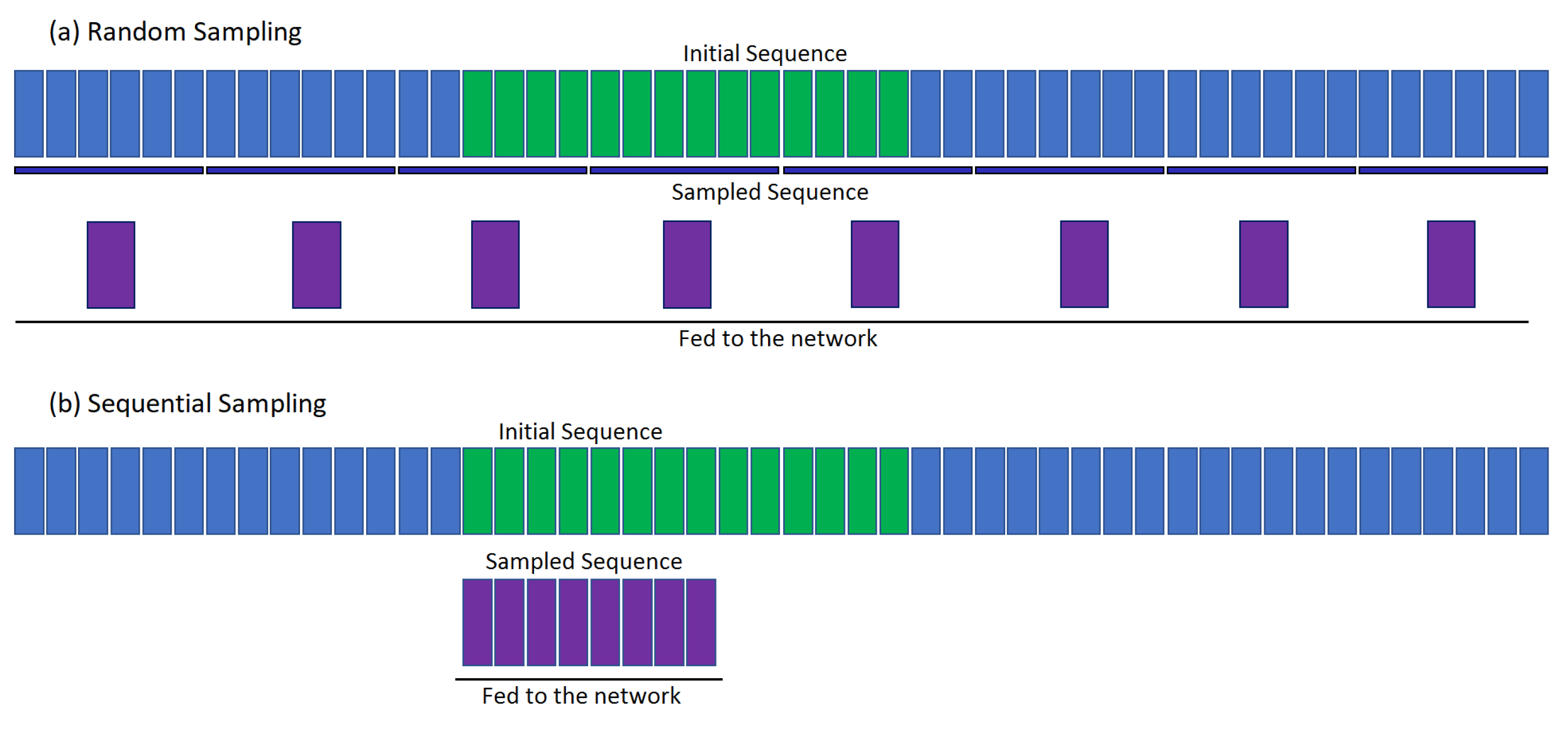
The input images were obtained by sampling down the acquired videos to n-images (4, 8, 12, or 16) with either the random sampling (RS) [
7] or sequential sampling (SS) technique. In random sampling, the image sequence is temporally separated into n-segments of equal size, and one image is sampled from each segment. This strategy helps the network to see the images from the entire temporal domain. In sequential sampling, n-images are sampled sequentially from a predefined starting point. By this strategy, the network is fed with sequential localized information from the region of interest. The starting point for this strategy was selected at a point after the first appearance of the droplet. Therefore, the images can be sampled from the initial region of dispense where there are a significant number of changes in the shape of droplets or these can be from a later part in the sequence where the droplet is mostly spherical.
Figure 5 illustrates both sequential and random sampling techniques.
4. Results and Discussions
The first tests were performed on deeper architectures. These networks were trained for 70 epochs. 3D-Resnet18, ECO Lite, and ECO Full had 87.40%, 87.62%, and 89.68% respective accuracies. Extensive testing was not performed on these architectures because they were overfitting. The rest of this section compares the shallower architectures, compares the sampling strategies, analyzes the effect of data cleaning, and analyzes the effect of adding the third acquisition batch. All these tests use eight segments.
4.1. Comparing Shallower Architectures
As there were various reasons (sampling strategy, data cleaning, and the number of batches used for training) which may lead to different accuracies for the same neural network architecture, this section compares the performance of the networks over these variables.
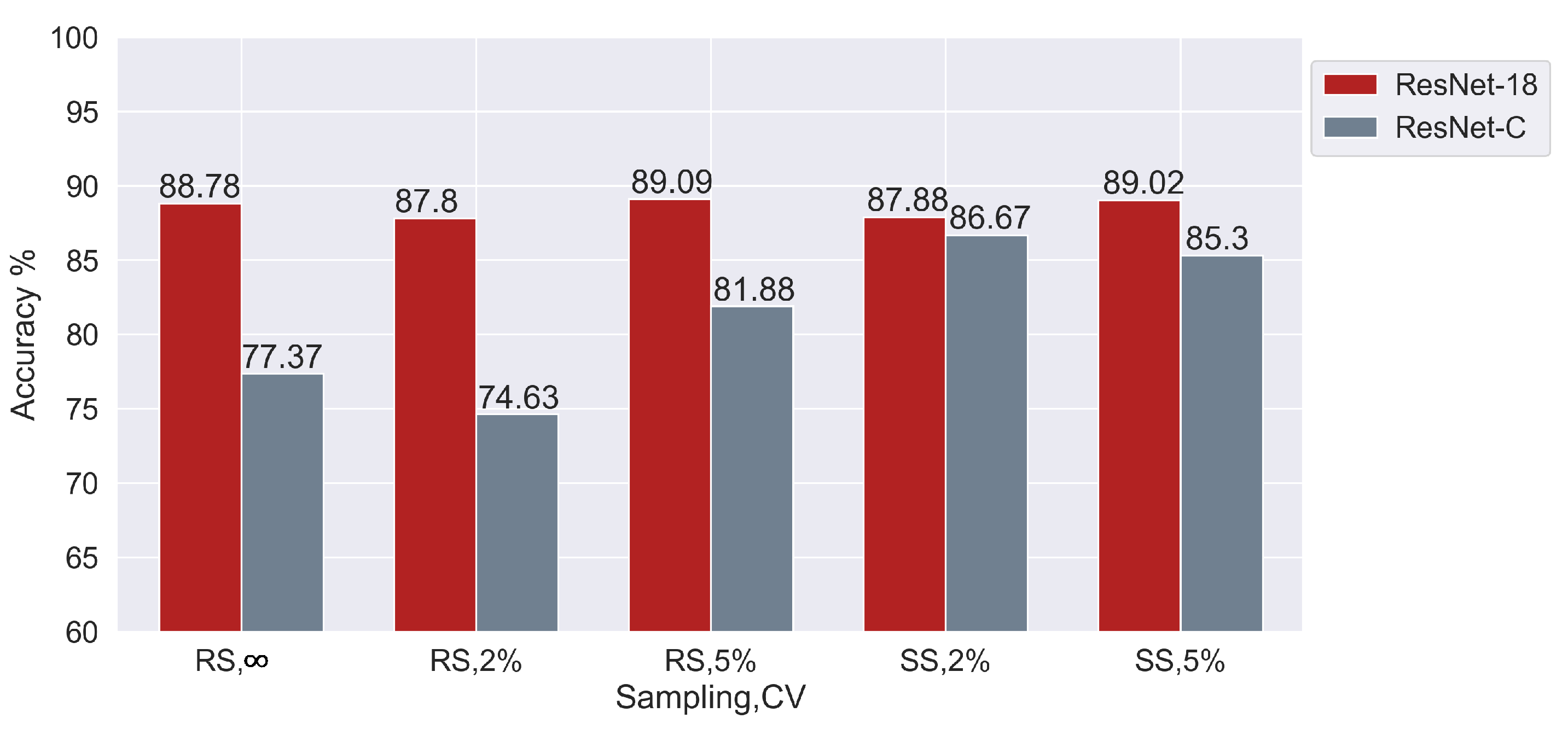
Figure 6 compares the pure 2D architectures on various filtering intensities (expressed as CV thresholds) and sampling conditions. ResNet-C has a lower performance as compared to ResNet-18. This shows that, for the current task, the higher number of layers in ResNet-18 makes it better at extracting the underlying features for every sampling and cleaning condition.
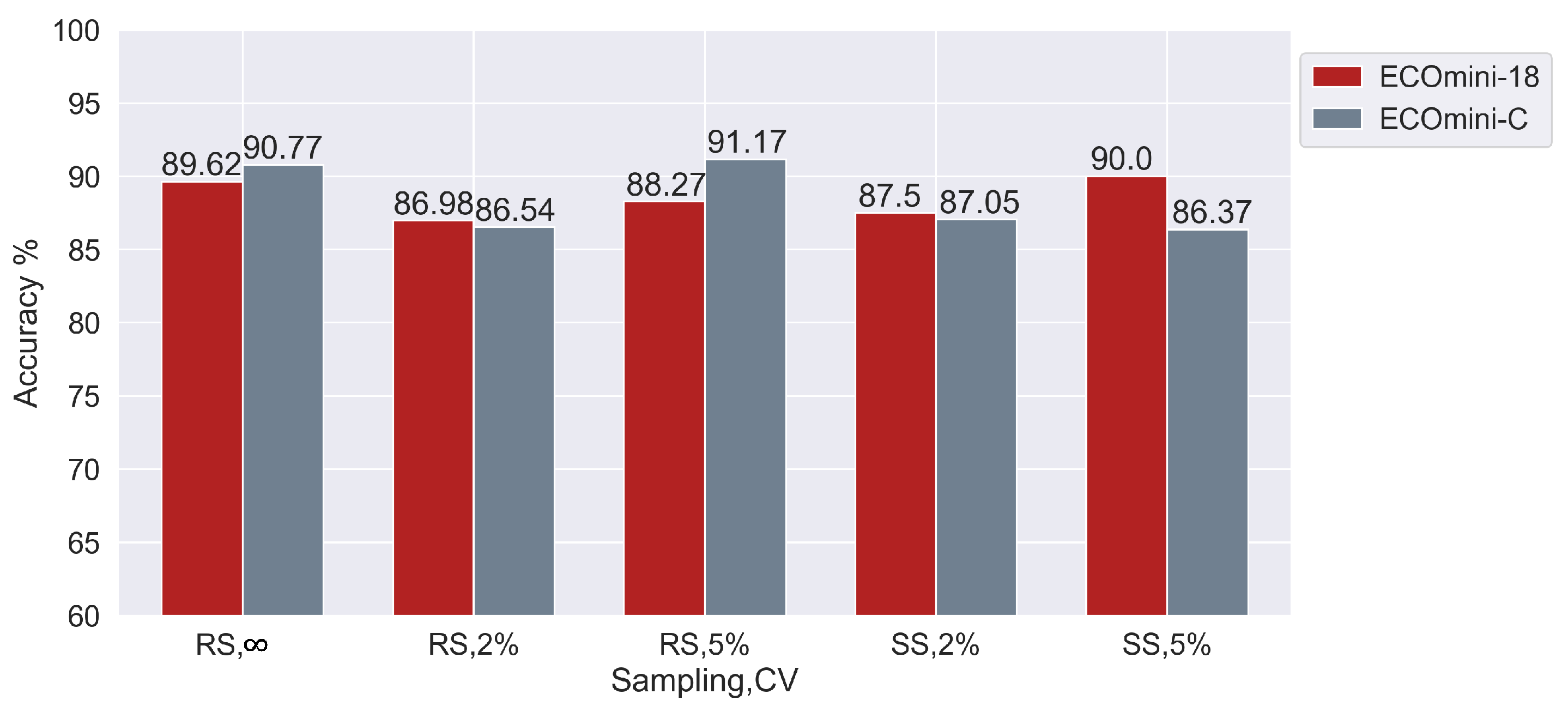
Next,
Figure 7 compares ECOmini-18 and ECOmini-C on various CV and sampling conditions. ECOmini-18 and ECOmini-C showed similar performance on the given dataset. This shows that adding the 3D layers with the ResNet-C helps it to extract more useful information from the current dataset.
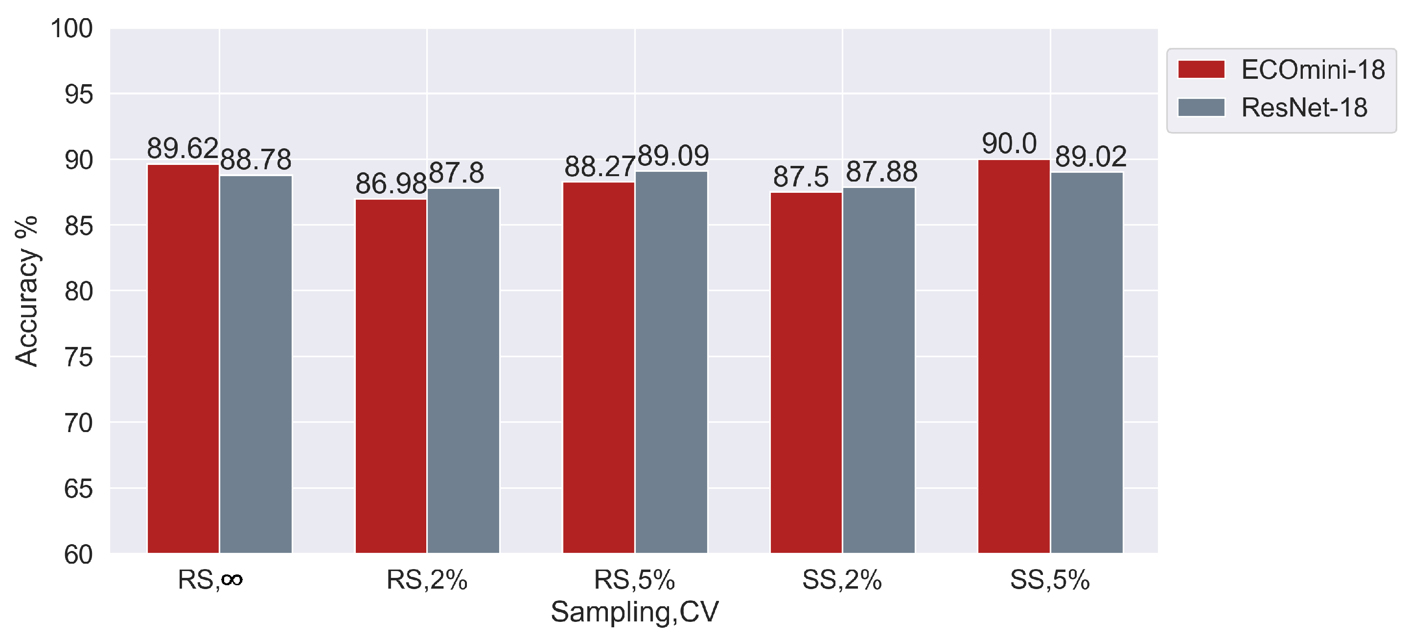
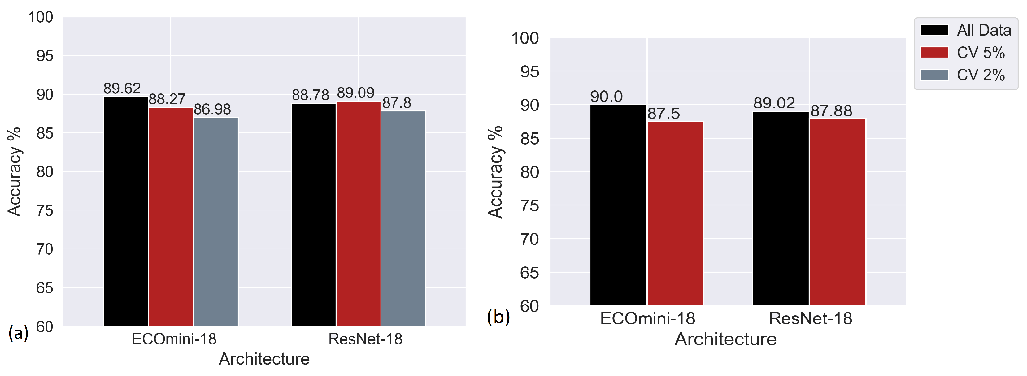
To analyze the effect of adding a 3D component with a good 2D extractor, a comparison between ECOmini-18 and ResNet-18 is shown in
Figure 8. ECOmini-18 and ResNet-18 showed similar performance. This shows that the spatiotemporal trajectories produced during dispensing at the current
Oh produce distinct enough underlying frames that the 2D components extracted by ResNet-18 alone are enough for the classification task. A high difference between the
Oh leads to very different underlying images [
4]; hence, the current 2D extractors can differentiate between the
Oh based on the single frames. Hence, for datasets similar to the one used in this study where the difference in the
Oh is large, a 2D architecture can be used to make inferences with a single frame.
4.2. Comparing Sampling Strategies
Depending on the non-contact dispensing parameters, the droplets had a different first frame of appearance and were dispensed at different velocities. These lead to a different number of empty frames before the dispense and after the droplet had left the region of interest. Therefore, a random sampling strategy can have a significant number of empty frames.
Figure 9 shows a performance comparison between ResNet-18 and ECOmini-18 while using the two sampling strategies.
In the case of ResNet-18, both sampling strategies had very similar performances. As it is a 2D architecture, ResNet-18 does not extract any patterns that exist between the frames. Hence, it is not affected by the type of sampling, whereas in the case of ECOmini-18, sequential sampling outperforms random sampling for the current dataset. This can be because, for the current dataset, the useful information on shape evolution lies in the initial part of the dispenses. To verify this, sequential sampling with different offsets was performed.
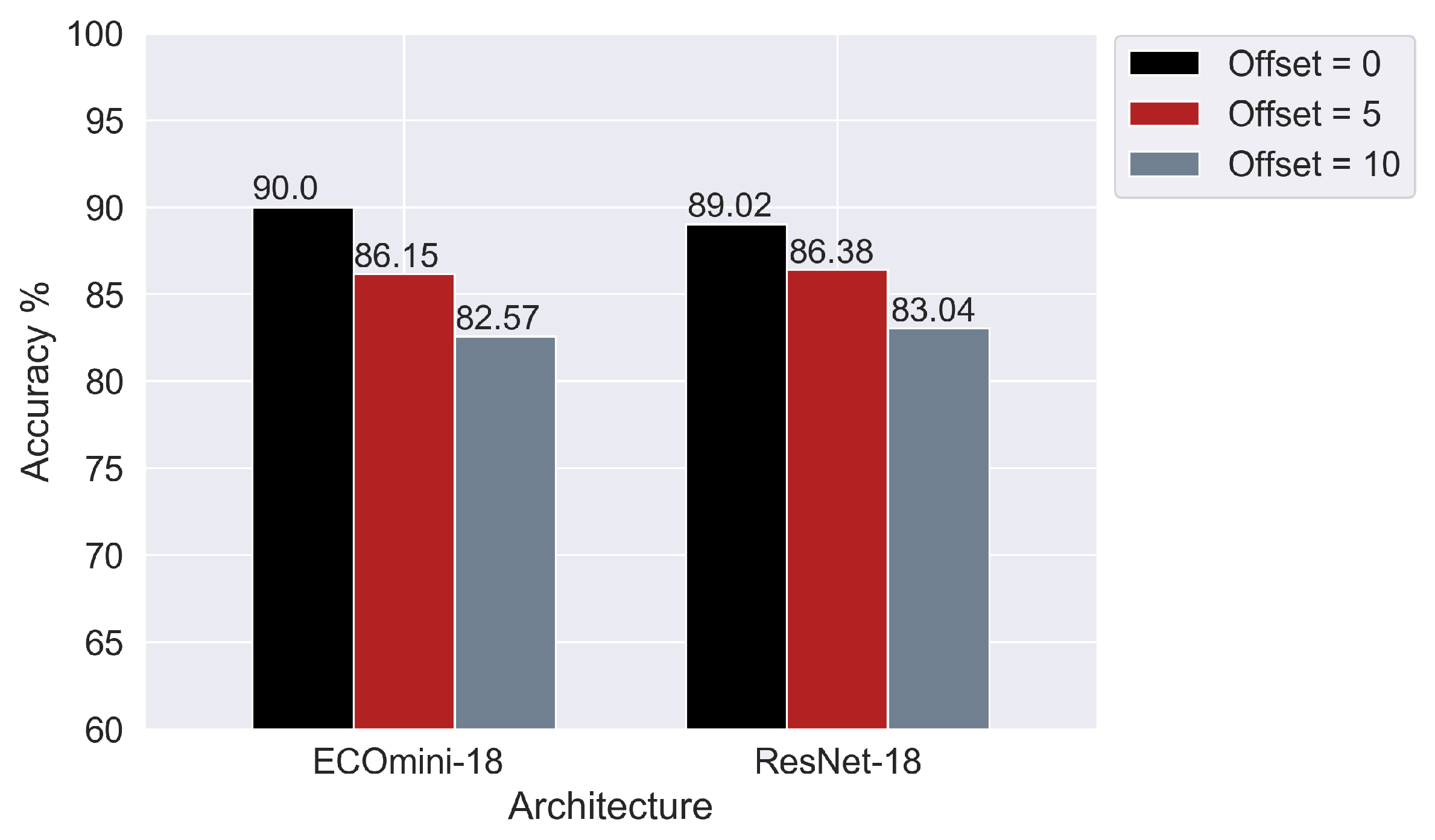
Figure 10 shows a sequential sampling of eight frames with no offset, a five-frame offset, and a ten-frame offset for ECOmini-18 and ResNet-18.
The neural networks perform the best when fed with images from the initial part of the sequence. Hence, the relevant information is relatively more localized in the initial part of the sequences.
4.3. Effect of Data Cleaning
The data were cleaned based on the CV of the droplet mass obtained within the 25 repeats of the same dispenser configuration. The lower the CV threshold, the lower the amount of remaining data. It is worth noting that CV
∞ represents the uncleaned data.
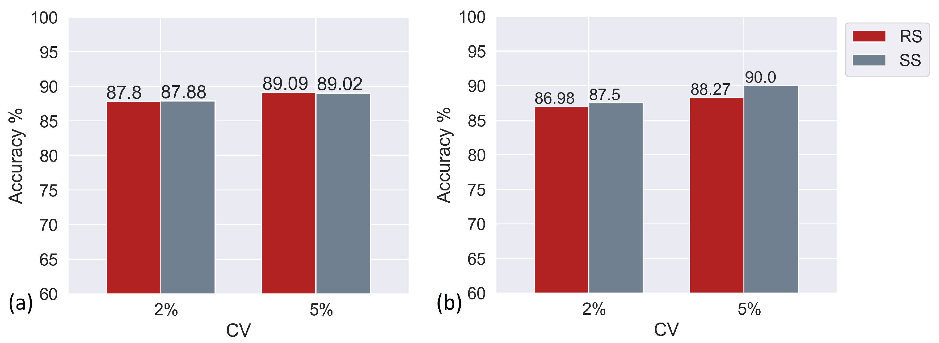
Figure 11 compares the performance of the ECOmini-18 and ResNet-18 over different CV thresholds and sampling strategies.
The performance of the neural networks decreases with the decrease in the amount of data as the amount of filtering is increased.
4.4. Effect of Adding New Acquisition Batch
Training on more than one acquisition batch helps the network reduce the shortcut learning that can arise by training on a single batch. The increase in the amount of diverse data helps the neural network to better generalize.
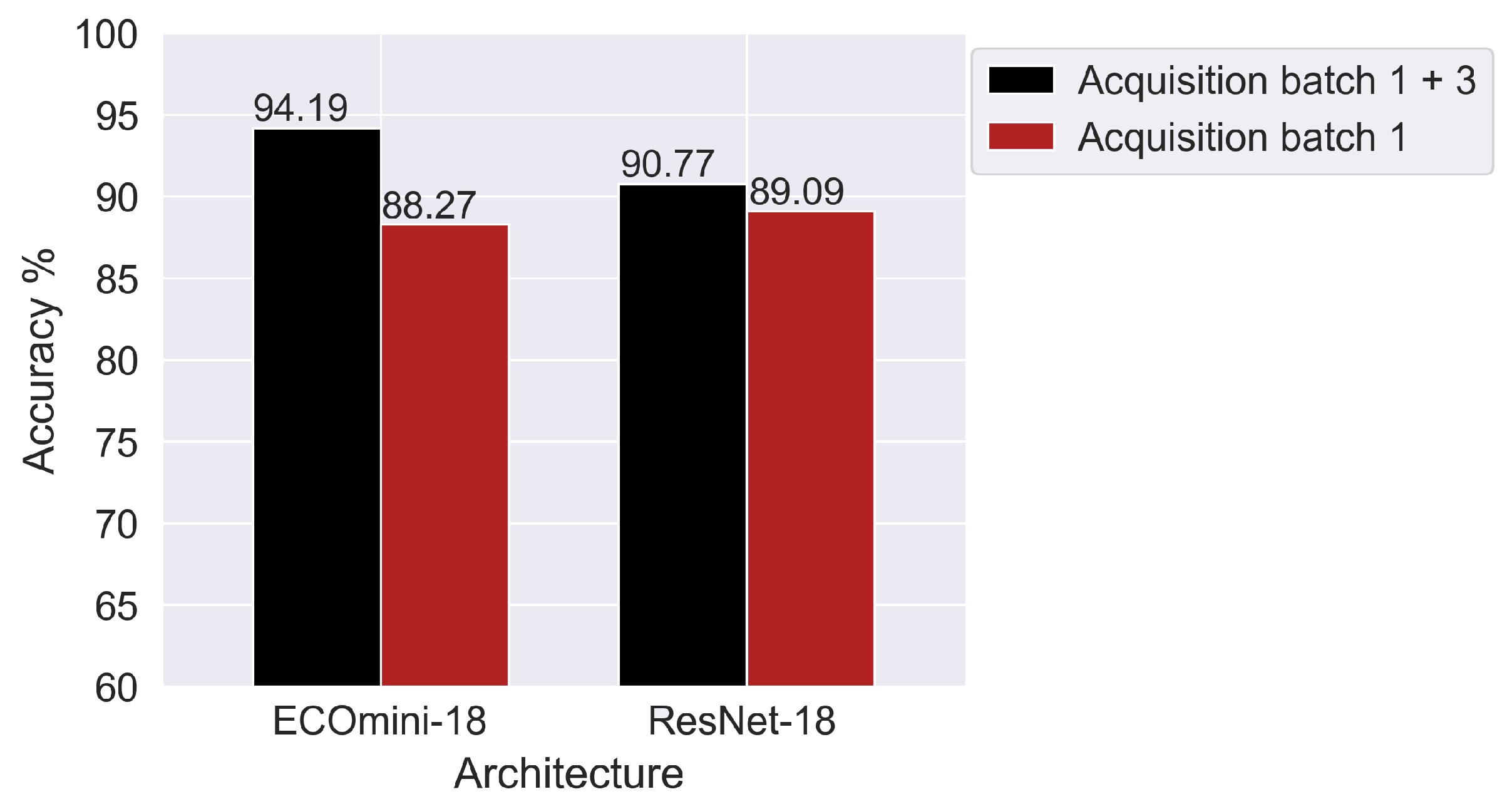
Figure 12 shows a comparison between the networks trained on a single acquisition batch and the networks trained on two acquisition batches. The data here are cleaned with a CV threshold of 5%.
The performance of the neural networks increases when the training is performed on acquisition batch 1 and 3 jointly. The ECOmini-18 model obtained by training on acquisition batch 1 and 3 jointly was the best model in the entire study.
5. Conclusions
The current work compares seven different neural network architectures over different sampling techniques, data cleaning conditions, and number of acquisition batches. In conclusion, deeper architectures (such as ECO Full) tend to overfit while finding the Ohnesorge number from dispensed droplet images. A shallower architecture with both 2D and 3D convolutions (ECOmini-18) performs slightly better than a shallower architecture with only 2D convolutions (ResNet-18). Though it has a slightly lower accuracy, inference can be made using ResNet-18 with as little as one image. The results also show that the CNNs with both 2D and 3D convolutions perform better when the frames are sampled sequentially, starting from the frame of the first appearance of the droplet. Next, it can be seen that data cleaning causes a decrease in classification accuracy due to a reduction in the amount of training data. Lastly, it can be seen that training on more than one acquisition batch improves the accuracy of the trained model. ECOmini-18 showed the maximum accuracy of 94.2%, trained on data from acquisition batches 1 and 3 jointly. This study is a proof-of-concept for neural networks to predict Ohnesorge numbers from droplet images. Moving forward, the technique can be further developed into a regression task, where the Ohnesorge number is a continuous scalar, instead of restricted to discrete classes. The CNNs can further be applied to other applications such as predicting the pinch-off time. Furthermore, the current CNNs can be trained in a physics-informed setup, reducing the size of datasets and biases from the experimental data.


 ,
, 


