Computation of Kinematic and Magnetic α-Effect and Eddy Diffusivity Tensors by Padé Approximation

Abstract

We present examples of Padé approximations of the $\alpha$-effect and eddy viscosity/diffusivity tensors in various flows. Expressions for the tensors derived in the framework of the standard multiscale formalism are employed. Algebraically, the simplest case is that of a two-dimensional parity-invariant six-fold rotation-symmetric flow where eddy viscosity is negative, indicating intervals of large-scale instability of the flow. Turning to the kinematic dynamo problem for three-dimensional flows of an incompressible fluid, we explore the application of Padé approximants for the computation of tensors of magnetic $\alpha$-effect and, for parity-invariant flows, of magnetic eddy diffusivity. We construct Padé approximants of the tensors expanded in power series in the inverse molecular diffusivity $1/\eta$ around $1/\eta =0$. This yields the values of the dominant growth rate to satisfactory accuracy for $\eta$, several dozen times smaller than the threshold, above which the power series is convergent. We do computations in Fortran in the standard “double” (real*8) and extended “quadruple” (real*16) precision, and perform symbolic calculations in Mathematica.

1. Introduction

Power series expansion of analytic functions is perhaps the most powerful tool of numerical analysis. Let us just note that most algorithms for the numerical integration of ordinary differential equations, such as the Runge–Kutta methods, rely on Taylor series expansions for derivation. The truncated series—i.e., polynomials—are easy to compute, and thus provide an important basic algorithm for the evaluation of many analytic functions.

However, there are two caveats. One is related to the finite precision of computations, stemming from the hardware architecture and employed in the overwhelming majority of computer codes. A well-known example of the resultant failure of a computational procedure is the straightforward attempt to compute an exponent of a real large negative number by this technique [1]. Mathematically, this does not present any difficulty—the large individual terms in the Taylor expansion around zero are guaranteed to mutually cancel out and yield the final result, which is less than unity. For finite-precision computations, however, the cancellation is no longer guaranteed, and the initial growth of individual terms can result in the ultimate loss of accuracy.

The other stems from the finiteness of the radius of convergence of most power series encountered in computational practice. A complementary technique is then needed to analytically continue a function defined by the power series outside its circle of convergence. This can be achieved by constructing the so-called Padé approximants [2,3,4], i.e., an implementation of the continuation in the form of the ratio of two polynomials. Let us cite the words of appraisal in [5]: “Padé approximation has the uncanny knack of picking the function you had in mind from among all the possibilities. Except when it doesn’t! That is the downside of Padé approximation: it is uncontrolled. There is, in general, no way to tell how accurate it is, or how far out in x it can usefully be extended. It is a powerful, but in the end still mysterious, technique”.

A no less mysterious notion is that of eddy diffusivity [6], also known as eddy (or turbulent) viscosity when fluid viscosity, the source of diffusion in hydrodynamics, is considered. Like the magnetic $\alpha$-effect and anisotropic kinetic alpha (AKA)-effect, eddy diffusivities are often encountered in magnetohydrodynamics when the generation of large-scale magnetic fields by flows of electrically conductive fluids is considered. At first sight, it is in direct contradiction with the second principle of thermodynamics. Of course, in fact no physical laws are violated. Both notions just describe the mean influence of the small scales on large-scale structures.

According to the modern paradigm, cosmic magnetic fields (such as the solar or geomagnetic field) exist due to the dynamo processes in the moving, electrically conductive medium (such as melted rocks in the outer Earth’s core) [7]. The generating flows are typically turbulent and feature a vast hierarchy of spatial and temporal scales. Small-scale fluctuations of the flow (called “cyclonic events” by Parker) give rise to small fluctuations in the magnetic field. The interaction of the small-scale components of the magnetic field and the flow velocity produces a mean electromotive force (e.m.f.) that may have a non-zero component parallel to the mean magnetic field, and this can be beneficial for magnetic field generation [8]. The part of the mean e.m.f. linear in the mean field gives rise to the so-called magnetic $\alpha$-effect. If the flow is parity-invariant, the $\alpha$-effect disappears and the impact of yet smaller spatial scales becomes apparent; the mean e.m.f. is then a linear combination of the first-order spatial derivatives of the mean field, giving rise to eddy (turbulent) diffusivity. These physical ideas are treated under various simplifying assumptions in mean-field electrodynamics [9,10], and relying only on the first principles, by asymptotic methods of homogenization of elliptic operators in magnetohydrodynamic multiscale stability theory [11,12,13,14,15,16,17]. Weakly nonlinear stability problems are also amenable to these methods [18].

The analysis of equations makes it evident that eddy viscosity/diffusivity acquires unusual properties because it acts on mean fields only, i.e., essentially an open physical system is considered. In fact, in this class of MHD systems, the inverse energy cascade is important, with energy proliferating from small scales toward large ones; the source of energy for the developing large-scale magnetic, hydrodynamic, or combined MHD perturbation is the forcing applied to maintain the perturbed (also sometimes called basic) fluid flow.

Evaluation of the $\alpha$-effect and eddy diffusivity tensors involves solving the so-called auxiliary problems, which are linear problems for the respective elliptic operators of linearization. In the large-scale dynamo problem, computing the magnetic $\alpha$-effect tensor requires considering three such problems; the number increases to 12 when the tensor of eddy diffusivity is sought (unless auxiliary problems for the adjoint operator come into play, decreasing the number of auxiliary problems to be treated to just 6, see, e.g., [19,20]). Interesting results (e.g., instability to large-scale perturbation or dynamos) are typically obtained for relatively small molecular viscosity or magnetic diffusivity. Consequently, high spatial resolution is needed when solving the auxiliary problems, which makes the problems computationally intensive. However, the tensors can be easily expanded in the respective Reynolds number (i.e., in the inverse viscosity or diffusivity, provided the size of the flow periodicity box and the flow velocity are order unity) when it is small, i.e., for large viscosities and diffusivities. When the parameter tends to the critical value for the onset of the small-scale instability (i.e., in the dynamo context, to the value for which the generation of small-scale magnetic fields starts), the tensors usually exhibit singular behavior [20,21,22,23] of a simple pole type, bounding from above the radius of convergence of the series. This suggests trying Padé approximants for computing the tensors and the respective large-scale magnetic field/instability growth rates.

Here, we report numerical experiments exploring these ideas. The paper is organized as follows. In Section 2, we apply the Padé approximants techniques for evaluation of the eddy viscosity in a two-dimensional flow with two symmetries, in whose presence the eddy viscosity tensor reduces to a scalar. In view of the first caveat discussed in the beginning of this introduction, we have chosen to perform the calculations in precise arithmetics allowing an arbitrary number of correct digits; for this purpose, we have used the programming language Mathematica, giving an opportunity to make symbolic computations. In Section 3, we revert to the standard “double precision” computations (real*8, in Fortran speak) of the magnetic $\alpha$-effect tensor, using the “quadruple precision” (real*16) computations for comparison. In Section 4, we again employ the symbolic capabilities of Mathematica to evaluate the magnetic eddy diffusivity tensor. Our findings are summarized in Section 5.

2. Calculation of Eddy Viscosity

No truly two-dimensional flows exist in nature, but they mimick properties of natural objects, such as the atmosphere or ocean [24,25,26]. We analyze the eddy viscosity tensor, ${\epsilon }_{ijk\ell }$ [11], of a two-dimensional flow of incompressible fluid that has two symmetries: parity invariance ($S1$) and six-fold rotation symmetry ($S2$).

Since an $S1$-symmetric flow has a center of symmetry, it cannot possess the large-scale anisotropic kinetic $\alpha$-effect [27]. This is important because in the presence of the AKA effect, the large-scale dynamics are essentially dispersive and non-diffusive, concealing the impact of the eddy viscosity. The symmetry $S2$ implies the isotropy of fourth-order tensors (see, for instance, [28]), in particular, ${\epsilon }_{ijk\ell }={\nu }_{\mathrm{E}}{\delta }_{ij}{\delta }_{k\ell }$, where the scalar ${\nu }_{\mathrm{E}}$ is the (standard) eddy viscosity and ${\delta }_{mn}$ is the Kronecker symbol. Although the assumption that a flow features the two symmetries is mathematically convenient, it may be non-realistic when considering natural or engineering problems [29].

Two-dimensional flows endowed with the symmetries $S1$ and $S2$ can be constructed as follows. A space-periodic flow is assumed, the periodicity cell being the rectangle

$$[0,L_1]\times [0,L_2]\ni \mathbf{x}=(x_1,x_2),L_1=\sqrt{3}{L}_2=2\pi .$$

Its stream-function $\mathsf{\Psi }(t,\mathbf{x})$ is then a sum of Fourier modes whose wave vectors are $p(2,0)+q(1,\sqrt{3})$, where p and q are integers. Any two such modes that have wave vectors mutually related by rotations by $\pi /3$ must both be involved in the sum with the same real amplitude.

We begin this section by recalling the expression for scalar eddy viscosity in terms of the solutions to two auxiliary problems and the analytical framework for evaluating the expansion of the eddy viscosity tensor in powers of the inverse of the molecular viscosity. We carry on by recalling the standard terminology and definitions of Padé approximants to a series. Finally, we discuss our results and conclusions.

2.1. Eddy Viscosities and Multiscale Techniques

For parity-invariant and six-fold rotation-symmetric flows of an incompressible fluid, eddy viscosities were calculated in [11] by multiscale techniques. They can be expressed in terms of solutions to two auxiliary problems, which can be solved analytically only in special cases [11] (e.g., if the flow depends only on a single spatial coordinate).

Briefly, the eddy viscosity in an isotropically forced two-dimensional flow is calculated as follows [11,30]. In terms of the stream-function $\mathsf{\Psi }(t,\mathbf{x})$, the two-dimensional forced Navier–Stokes equation for incompressible fluid takes the form

$${\partial }_t{\nabla }^2\mathsf{\Psi }+J({\nabla }^2\mathsf{\Psi },\mathsf{\Psi })=\nu {\nabla }^2{\nabla }^2\mathsf{\Psi }+\partial f_1/\partial x_2-\partial f_2/\partial x_1.$$

Its solution, $\mathsf{\Psi }$, defines a basic flow. Here, $J(g_1,g_2)=(\partial g_1/\partial x_1)(\partial g_2/\partial x_2)-(\partial g_1/\partial x_2)(\partial g_2/\partial x_1)$ is the Jacobian determinant of functions $g_1(x_1,x_2)$ and $g_2(x_1,x_2)$, the operator ${\nabla }^2={\partial }^2/\partial x_1^2+{\partial }^2/\partial x_2^2$ is the Laplacian, $\nu$ the kinematic molecular viscosity, and $\mathbf{f}=(f_1,f_2)$ the external force. (In our numerical examples, the flow norm and the size of the small-scale periodicity cell are order unity; thus, the inverse molecular viscosity can be regarded as the local Reynolds number, which is the key dimensionless parameter of the problem.) Now assume that the basic flow possesses the symmetries $S1$ and $S2$. Then the (scalar) eddy viscosity coefficient, ${\nu }_{\mathrm{E}}={\nu }_{\mathrm{E}}(\mathsf{\Psi },\nu )$, which depends only on the basic flow and molecular viscosity, is [30]

$${\nu }_{\mathrm{E}}(\mathsf{\Psi },\nu )=\nu -〈\left(Q+2\frac{\partial S}{\partial x_1}\right)\frac{\partial \mathsf{\Psi }}{\partial x_2}〉.$$

(1)

Here, the angle brackets denote the average over the periodicity cell,

$$〈g(x_1,x_2)〉=\frac{1}{L_1{L}_2}{\int }_{x_1=0}^{L_1}{\int }_{x_2=0}^{L_2}g(x_1,x_2)\mathrm{d}{x}_2\mathrm{d}{x}_1,$$

the scalar functions $Q(x_1,x_2)$ and $S(x_1,x_2)$ are solutions to two auxiliary problems

$$\mathfrak{G}Q=\frac{\partial {\nabla }^2\mathsf{\Psi }}{\partial x_2},\mathfrak{G}S=Q\frac{\partial {\nabla }^2\mathsf{\Psi }}{\partial x_2}+2J\left(\mathsf{\Psi },\frac{\partial Q}{\partial x_1}\right)-{\nabla }^{2}Q\frac{\partial \mathsf{\Psi }}{\partial x_2}+4\nu \frac{\partial {\nabla }^{2}Q}{\partial x_1},$$

(2)

and $\mathfrak{G}$ denotes the linearization of the Navier–Stokes equation around $\mathsf{\Psi }$,

$$\mathfrak{G}:\psi \mapsto J({\nabla }^2\psi ,\mathsf{\Psi })+J({\nabla }^2\mathsf{\Psi },\psi )-\nu {\nabla }^2{\nabla }^2\psi .$$

We restrict it to zero-mean functions of the same space periodicity as the basic flow. In this functional space, we can define the inverse Laplace operator, which we denote as ${\nabla }^{-2}$. A field G from this space can be expressed as a Fourier series

$$G(x_1,x_2)=\sum _{p,q\in \mathbb{Z}}{\widehat{G}}_{p,q}exp\left(2\pi \mathrm{i}(p{x}_1/L_1+q{x}_2/L_2)\right),$$

(3)

where $〈G〉={\widehat{G}}_{0,0}=0.$ The equation ${\nabla }^{2}F=G\iff F={\nabla }^{-2}G$ can now be readily solved: given $〈F〉=0$, we find

$${\nabla }^{-2}G=-{\left(2\pi \right)}^{-2}\sum _{p,q\in \mathbb{Z}\setminus \left\{0\right\}}\frac{{\widehat{G}}_{p,q}}{{(p/L_1)}^2+{(q/L_2)}^2}exp\left(2\pi \mathrm{i}(p{x}_1/L_1+q{x}_2/L_2)\right).$$

(4)

The existence of a deterministic time-independent space-periodic flow, which has an isotropic negative eddy viscosity when the molecular viscosity is below a critical value, was established in [31]. The so-called decorated hexagonal flow (DHF), on which we will also focus here, is

$$\begin{array}{cc}\mathsf{\Psi }(x_1,x_2)=[\hfill & -cos2x_1-cos(x_1+\sqrt{3}{x}_2)-cos(x_1-\sqrt{3}{x}_2)\hfill \\ & +cos(4x_1+2\sqrt{3}{x}_2)+cos(5x_1-\sqrt{3}{x}_2)+cos(x_1-3\sqrt{3}{x}_2)\hfill \\ & -cos4x_1-cos(2x_1+2\sqrt{3}{x}_2)-cos(2x_1-2\sqrt{3}{x}_2)\hfill \\ & +cos(4x_1-2\sqrt{3}{x}_2)+cos(5x_1+\sqrt{3}{x}_2)+cos(x_1+3\sqrt{3}{x}_2)]/2.\hfill \end{array}$$

(5)

The phenomenon of negative eddy viscosity is quite common among two-dimensional divergenceless space-periodic basic flows with the symmetries $S1$ and $S2$: about 1/3 of such flows feature negative eddy viscosity for sufficiently low molecular viscosity [30]. The auxiliary problems (2) can be solved either numerically by spectral methods or by expanding in powers of ${\nu }^{-1}$ to high orders and afterwards extending analytically (relying on their meromorphy  [30]) beyond the disk of convergence. We examine the latter method, enabling us to perform all calculations exactly.

2.2. Eddy Viscosity Expansion in Powers of ${\nu }^{-1}$

Let us expand (1):

$${\nu }_{\mathrm{E}}(\mathsf{\Psi },\nu )=\nu +\sum _{n=1}^{\infty }{\nu }_{\mathrm{E}}^{\left(n\right)}\left(\mathsf{\Psi }\right){\nu }^{-n}.$$

(6)

To calculate ${\nu }_{\mathrm{E}}^{\left(n\right)}$, we expand the solutions Q and S to (2) in Maclaurin series in ${\nu }^{-1}$:

$$Q=\sum _{n=1}^{\infty }{Q}^{\left(n\right)}{\nu }^{-n},S=\sum _{n=1}^{\infty }{S}^{\left(n\right)}{\nu }^{-n}.$$

Substituting the series into (1) and integrating by parts yields

$${\nu }_{\mathrm{E}}^{\left(n\right)}\left(\mathsf{\Psi }\right)=〈-Q^{\left(n\right)}\frac{\partial \mathsf{\Psi }}{\partial x_2}+2S^{\left(n\right)}\frac{{\partial }^2\mathsf{\Psi }}{\partial x_1\partial x_2}〉.$$

(7)

Here, $Q^{\left(1\right)}=-{\nabla }^{-2}(\partial \mathsf{\Psi }/\partial x_2)$ and $S^{\left(1\right)}=-4{\nabla }^{-2}(\partial Q^{\left(1\right)}/\partial x_1),$ and the subsequent terms satisfy the recurrence relations:

$$Q^{\left(n\right)}=\mathfrak{B}{Q}^{(n-1)},$$

(8)

$$S^{\left(n\right)}=\mathfrak{B}{S}^{(n-1)}-{\nabla }^{-2}{\nabla }^{-2}\left[Q^{(n-1)}\frac{\partial {\nabla }^2\mathsf{\Psi }}{\partial x_2}+2J\left(\mathsf{\Psi },\frac{\partial Q^{(n-1)}}{\partial x_1}\right)-{\nabla }^2{Q}^{(n-1)}\frac{\partial \mathsf{\Psi }}{\partial x_2}+4\frac{\partial {\nabla }^2{Q}^{\left(n\right)}}{\partial x_1}\right],$$

(9)

where the operator $\mathfrak{B}$ is defined as

$$\mathfrak{B}:f\mapsto {\nabla }^{-2}{\nabla }^{-2}\left[J({\nabla }^{2}f,\mathsf{\Psi })+J({\nabla }^2\mathsf{\Psi },f)\right].$$

Since here we consider parity-invariant flows, their stream-functions being even, i.e., $\mathsf{\Psi }(-\mathbf{x})=\mathsf{\Psi }\left(\mathbf{x}\right)$, the series (6) involves only odd powers of ${\nu }^{-1}$ [30], i.e., ${\nu }_{\mathrm{E}}^{\left(n\right)}=0$ for all even n.

By definition, the $[L/M]$ Padé approximant to a series, whose first $m\ge L+M+1$ terms are known, is the ratio of a polynomial of degree $\le L$ to a polynomial of degree $\le M$, such that the first $L+M+1$ terms of the expansion of the ratio coincide with the respective terms of the series.

We use Padé approximants to reconstruct the dependence of the eddy viscosity on the inverse molecular viscosity employing the expansion (6). The Padé approximation techniques can also be naturally applied for exploring the poles of the eddy viscosity. A pole on the real axis can usually be linked to the onset of linear instability to small-scale perturbations, or sometimes (if it appears again on decreasing $\nu >0$) to its cessation.

2.3. Results of Calculations

The performance of present-day computers and efficiency of symbolic programming software gives an opportunity to calculate the coefficients (7) using recurrence relations (8)-(9) and construct the Padé approximants exactly. All calculations reported in this section are performed with full precision by Mathematica [32].

Table 1. The first 39 non-zero coefficients of (6) for the decorated hexagonal flow (DHF, prime decomposition where presented). The first 5 significant figures of these coefficients are given in [31]. $“a⋘p⋙c”$ denotes a natural number containing p decimal digits between a and b.

n	Coefficient ${\mathit{\nu }}_{\mathbf{E}}^{\left(\mathit{n}\right)}$ (Exact Rational Number)
1	$\frac{3}{2^2}$
3	$-\frac{3\times 5\times 11\times 1931\times 80491}{2^9\times 7^4\times {13}^2\times {19}^2}$
5	$-\frac{3\times {53}^2\times 222967\times 1994517983033813651288306079222192539}{2^{19}\times 5^2\times 7^9\times {13}^6\times {19}^7\times {31}^3\times {37}^2\times {43}^3\times {61}^2}$
7	$\frac{3^3\times 23\times 17401\times 11608063\times 570396658307516795186040829874710499\times 595146062519802577066082838776447096016784218965582671080441286999}{2^{25}\times 5^2\times 7^{17}\times {13}^{10}\times {19}^{11}\times {31}^5\times {37}^7\times {43}^5\times {61}^6\times {67}^3\times {73}^3\times {79}^3\times {97}^3\times {103}^2\times {109}^2}$
9	$-\frac{9606359879⋘188⋙5777697637}{2^{33}\times 5^2\times 7^{24}\times {11}^2\times {13}^{14}\times {19}^{15}\times {31}^7\times {37}^{11}\times {43}^7\times {61}^{10}\times {67}^5\times {73}^5\times {79}^5\times {97}^5\times {103}^3\times {109}^6\times {127}^3\times {139}^3\times {151}^3\times {157}^2\times {163}^2}$
11	$-\frac{7129561983⋘324⋙7108258721}{8493879641⋘326⋙4312960000}$
⋮	⋮
39	$-\frac{1648936106⋘9785⋙2091564067}{3775138782⋘9788⋙0000000000}$

shows some of the first twenty non-zero coefficients ${\nu }_{\mathrm{E}}^{\left(n\right)}$ ($n=1,3,5,\dots ,39$) for the DHF. One of the reasons for performing full precision symbolic computations with Mathematica has been a hope of discovering useful relations between the coefficients of the approximants. Unfortunately, none are visible in the data in Table 1.

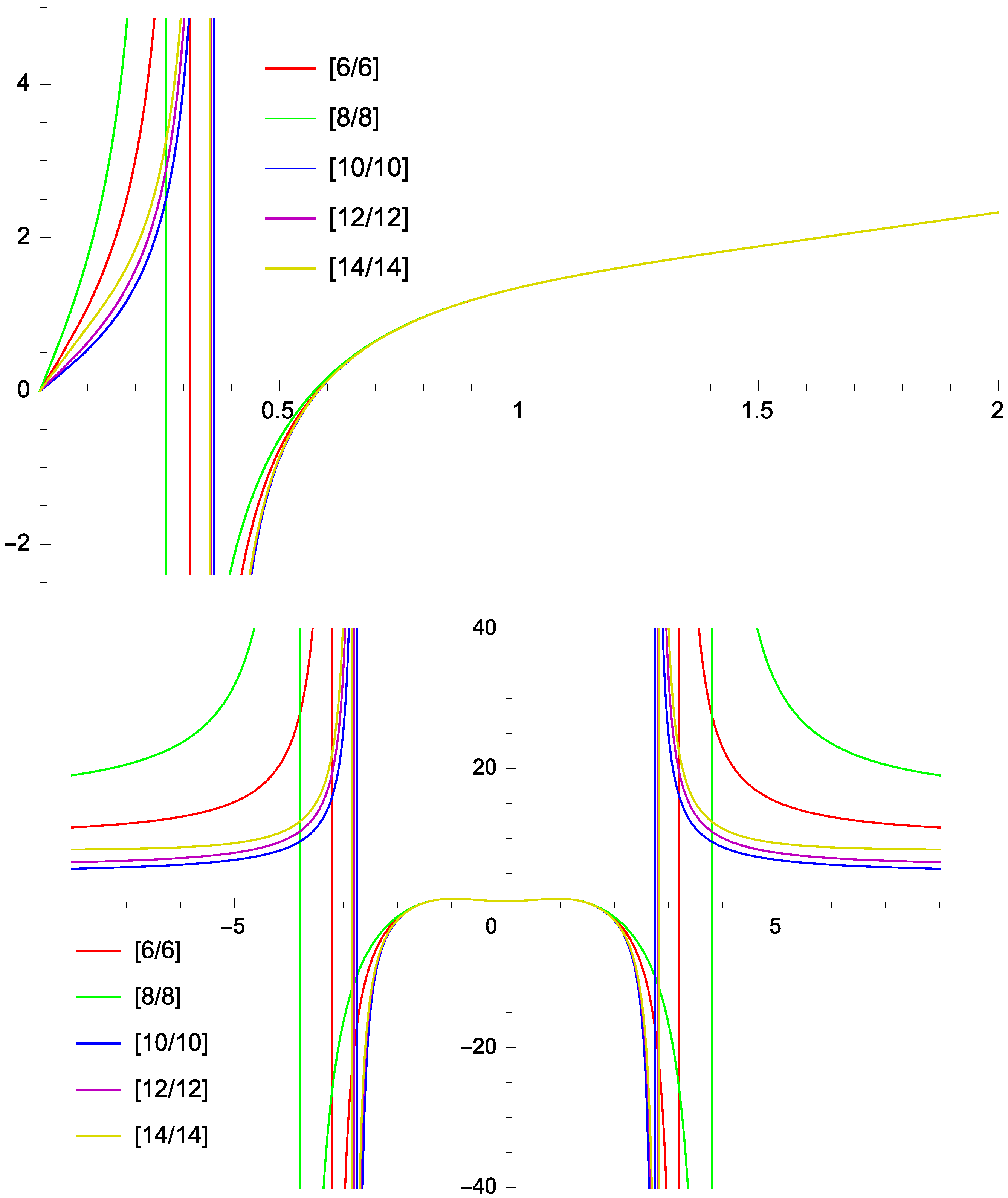
We truncate the series (6) at orders up to 39, even terms missing. Roots of their Padé approximants quickly stabilize near $\nu ={\nu }^{\star }\approx 0.58$ (see Figure 1), indicating a transition to negative eddy viscosity at lower molecular viscosities. The root ${\nu }^{\star }$ is simple; a sharpened estimate is $1/{\nu }^{\star }=1.72144\pm {10}^{-5}$.

These results indicate that Padé approximants are a reliable alternative to other methods for the calculation of the point of the onset of large-scale instability in this type of flow. Not only do they furnish stable estimates (provided the approximated function is meromorphic and the series is long enough), but they also serve as precursors to future work. An illustration is Figure 1 (right), where the $[14/14]$ approximant (as many others) exhibits a singular behavior near $1/\nu \approx 2.81$ apparently related to the onset of linear instability to small-scale perturbations. The non-monotonicity of the eddy viscosity as a function of $\nu$ can be regarded as a manifestation of the complexity of the two-dimensional turbulent flow.

3. Computation of the Magnetic $\mathit{\alpha }$-Effect Tensor

As we have seen in the previous section, the use of Padé expansions for reconstructing the dependence of eddy viscosity on the molecular one is possible and does not require very high degrees of the polynomials involved, at least for moderate (not very small) molecular viscosities. However, for 3D fields, arbitrary-precision symbolic calculations cannot be regarded as a practical realization of the approximation algorithm. Here, we construct Padé approximants for evaluation of the magnetic $\alpha$-effect tensor using arithmetics of floating point numbers of the conventional double (real*8) and the extended quadruple (real*16) precision. The problem now at hand is to construct approximations applicable for small magnetic molecular diffusivities.

3.1. The Multiscale Formalism Revealing the Magnetic $\alpha$-Effect

We review here the multiscale expansions [17] describing the kinematic generation of large-scale magnetic fields by small-scale zero-mean space-periodic steady flows. Our magnetic modes depend on two three-dimensional spatial variables, the fast, $\mathbf{x}$, and slow, $\mathbf{X}=\epsilon \mathbf{x}$, one (the flow $\mathbf{v}$ depends exclusively on $\mathbf{x}$). A magnetic mode $\mathbf{b}$ is an eigenfield of the magnetic induction operator $\mathfrak{L}:$

$$\mathfrak{L}\mathbf{b}=\lambda \mathbf{b},$$

(10)

$$\mathfrak{L}:\mathbf{b}\mapsto \eta {\nabla }^2\mathbf{b}+\nabla \times (\mathbf{v}\times \mathbf{b}).$$

(11)

Here, $\eta$ is the magnetic molecular diffusivity and Re $\lambda$ the growth rate of the mode $\mathbf{b}$. Both the mode and flow are solenoidal.

The scale ratio $\epsilon$ is a small parameter of the problem, in which the magnetic mode $\mathbf{b}$ and its growth rate are expanded:

$$\mathbf{b}=\sum _{n=0}^{\infty }{\mathbf{b}}_n(\mathbf{X},\mathbf{x}){\epsilon }^n,$$

(12)

$$\lambda =\sum _{n=0}^{\infty }{\lambda }_n{\epsilon }^n.$$

(13)

By substituting the expansions into (10) and the solenoidality conditions, we derive a hierarchy of equations for the coefficients in (12) and (13).

As in the previous section, we denote by angle brackets the mean over the periodicity cell ${\mathbb{T}}^3$ in the fast variables and by the braces, the fluctuating part:

$$〈\mathbf{f}〉={\left(2\pi \right)}^{-3}{\int }_{{\mathbb{T}}^3}\mathbf{f}(\mathbf{X},\mathbf{x})\mathrm{d}\mathbf{x}=\sum _{k=1}^3{〈\mathbf{f}〉}_k{\mathbf{e}}_k,\left\{\mathbf{f}\right\}=\mathbf{f}-〈\mathbf{f}〉.$$

Here, ${\mathit{e}}_k$ are unit Cartesian coordinate vectors.

The relevant solution to the first (order ${\epsilon }^0$) equation $\mathfrak{L}{\mathbf{b}}_0={\lambda }_0{\mathbf{b}}_0$ is ${\lambda }_0=0$ and a linear combination ${\mathbf{b}}_0={\sum }_{k=1}^3{〈{\mathbf{b}}_0〉}_k{\mathbf{s}}_k$ of small-scale solenoidal neutral magnetic modes ${\mathbf{s}}_k\left(\mathbf{x}\right)$ that are solutions to the three so-called auxiliary problems of type I:

$$\mathfrak{L}{\mathbf{s}}_k=0,〈{\mathbf{s}}_k〉={\mathbf{e}}_k.$$

(14)

Averaging the second (order ${\epsilon }^1$) equation,

$$\mathfrak{L}{\mathbf{b}}_1+2\eta (\nabla ·{\nabla }_{\mathbf{X}}){\mathbf{b}}_0+{\nabla }_{\mathbf{X}}\times (\mathbf{v}\times {\mathbf{b}}_0)={\lambda }_1{\mathbf{b}}_0,$$

(15)

we obtain an eigenvalue problem

$${\nabla }_{\mathbf{X}}\times \left(\mathfrak{A}〈{\mathbf{b}}_0〉\right)={\lambda }_1〈{\mathbf{b}}_0〉,{\nabla }_{\mathbf{X}}·〈{\mathbf{b}}_0〉=0$$

(16)

(the subscript $\mathbf{X}$ denotes differentiation in the slow variables). Here, $\mathfrak{A}$ is the tensor of the magnetic $\alpha$-effect. The kth column of this $3\times 3$ matrix is

$${\mathfrak{A}}_k=〈\mathbf{v}\times {\mathbf{s}}_k〉,$$

(17)

in agreement with Parker’s [8] concept of the interaction of fine structures of the flow, $\mathbf{v}$, and magnetic field, ${\sum }_{k=1}^3{〈{\mathbf{b}}_0〉}_k\left\{{\mathbf{s}}_k\right\}$, giving rise to a mean e.m.f., $\mathfrak{A}〈{\mathbf{b}}_0〉$, linear in the large-scale magnetic field $〈{\mathbf{b}}_0〉$. For space-periodic mean fields

$$〈{\mathbf{b}}_0〉=\mathbf{B}{\mathrm{e}}^{\mathrm{i}\mathbf{q}·\mathbf{X}},\mathbf{B}·\mathbf{q}=0,$$

(18)

where $\mathbf{q}$ is an arbitrary unit vector, straightforward algebra [20] yields solutions to the eigenvalue problem (16):

$${\lambda }_{1_{\pm }}\left(\mathbf{q}\right)=\frac{\mathrm{i}}{2}\left(({\mathfrak{A}}_3^2-{\mathfrak{A}}_2^3)q_1+({\mathfrak{A}}_1^3-{\mathfrak{A}}_3^1)q_2+({\mathfrak{A}}_2^1-{\mathfrak{A}}_1^2)q_3\right)\pm \sqrt{a},a=\mathbf{q}·(det{}^{\mathrm{s}}\mathfrak{A}){{}^{\mathrm{s}}\mathfrak{A}}^{-1}\mathbf{q}.$$

(19)

Here, ${{}^{\mathrm{s}}\mathfrak{A}}_k^l=({\mathfrak{A}}_k^l+{\mathfrak{A}}_l^k)/2$ are entries of the symmetrized $\alpha$-tensor ${}^{\mathrm{s}}\mathfrak{A}=(\mathfrak{A}+{\mathfrak{A}}^{*})/2$.

For $a\le 0$, the $\alpha$-effect just sustains harmonic oscillations of the mean magnetic field in the slow time $T_1=\epsilon t$. When $a>0$, the slow-time growth rate Re ${\lambda }_1\left(\mathbf{q}\right)=\sqrt{a}$ of the large-scale magnetic mode depends only on the symmetrized tensor ${}^{\mathrm{s}}\mathfrak{A}$, whose eigenvalues ${\alpha }_i$ are real. In the Cartesian coordinate system, whose axes coincide with eigenvectors of ${}^{\mathrm{s}}\mathfrak{A}$, (19) takes the form

$$a={\alpha }_1{\alpha }_2{\left(q_3^{\prime }\right)}^2+{\alpha }_2{\alpha }_3{\left(q_1^{\prime }\right)}^2+{\alpha }_1{\alpha }_3{\left(q_2^{\prime }\right)}^2,$$

where $q_i^{\prime }$ are components of $\mathbf{q}$ in this basis. Thus,

$${\gamma }_{\alpha }\equiv \underset{\left|\mathbf{q}\right|=1}{max}\mathrm{Re}{\lambda }_{1_{\pm }}\left(\mathbf{q}\right)=\sqrt{max({\alpha }_1{\alpha }_2,{\alpha }_2{\alpha }_3,{\alpha }_1{\alpha }_3)}$$

(20)

is the maximum slow-time growth rate of large-scale magnetic modes generated by the $\alpha$-effect. While the entries of the $\alpha$-effect tensor, ${\mathfrak{A}}_l^k$, are smooth functions of $\eta$, the graph of ${\gamma }_{\alpha }$ (20) has cusps at the points $\eta$, where ${\alpha }_1<{\alpha }_2=0<{\alpha }_3$ [20] (see, e.g., two such cusps in Figure 2).

When $a\ne 0$ and the kernel of the magnetic induction operator $\mathfrak{L}$ does not involve small-scale zero-mean modes (generically both conditions are satisfied), all terms in the expansions (12) and (13) can be determined from the hierarchy of equations obtained by substituting the series into the eigenvalue Equation (10). If the symmetrized tensor ${}^{\mathrm{s}}\mathfrak{A}$ is positively or negatively defined (and if the spatial periodicity of the eigenfunction is compatible with that of the flow), then the series (12) and (13) are summable [16] for sufficiently small $\epsilon$ and constitute an analytical in the $\epsilon$ eigensolution for the large-scale magnetic induction operator; a unique $\epsilon$-parameterized branch of the eigenvalues (13) originates from any simple eigenvalue ${\lambda }_1$ of the $\alpha$-effect operator.

3.2. Padé Approximation

The modes ${\mathbf{s}}_k$ (and consequently, elements of the magnetic $\alpha$-effect tensor) are functions of molecular eddy diffusivity $\eta$, meromorphic in this parameter. (By contrast, the slow-time growth rates of modes generated by the $\alpha$-effect are not, because the square root present in (19) gives rise to branch points.) A power series expansion of ${\mathbf{s}}_k$ in ${\eta }^{-1}$ for large $\eta$ can be constructed like in the hydrodynamic problem considered in the previous section. We divide (14) by $\eta$ to obtain

$${\nabla }^2{\mathbf{s}}_k=-{\eta }^{-1}\nabla \times (\mathbf{v}\times {\mathbf{s}}_k).$$

Consequently, the coefficients in the expansion

$${\mathbf{s}}_k=\sum _{n=0}^{\infty }{\mathbf{s}}_k^{\left(n\right)}{\eta }^{-n}$$

(21)

satisfy the recurrence relations

$${\mathbf{s}}_k^{\left(0\right)}={\mathbf{e}}_k,{\mathbf{s}}_k^{\left(n\right)}=-{\nabla }^{-2}\left(\nabla \times (\mathbf{v}\times {\mathbf{s}}_k^{(n-1)})\right)\mathrm{for}n\ge 1$$

(22)

(cf. (5.14)–(5.15) in [13]). Here, ${\nabla }^{-2}$ denotes the inverse Laplacian in the fast variables acting in the functional space of zero-mean fields. (Actually, we consider the problem for a flow, whose r.m.s.  velocity is unity; the size of the periodicity box also being order unity, the inverse molecular diffusivity ${\eta }^{-1}$ can be regarded, like in the hydrodynamic case, to be equal to the local magnetic Reynolds number, the dimensionless parameter characterizing the mathematical properties of the problem. (21) can thus be understood as an expansion in a small Reynolds number.) These recurrence relations can be used to compute the coefficients in (21) by pseudospectral methods. It must be noted that mathematically, they are perfectly suitable for numerical work: indeed, the presence of the inverse Laplacian in the second relation (22) suggests that on increasing the number n of the coefficient ${\mathbf{s}}_k^{\left(n\right)}$, they become smoother and their energy spectrum decay is steeper. This is in sharp contrast, for instance, with the recurrence relations for the Lagrangian time-Taylor coefficients in the expansions of solutions to the Euler equation for incompressible fluid flow [33].

It is straightforward to determine the radius of convergence of the series (21), $\rho$, regarded as a function of $1/\eta$. The recurrence relations (22) involve the operator

$$\mathfrak{M}:\mathbf{s}\mapsto -{\nabla }^{-2}\left(\nabla \times (\mathbf{v}\times \mathbf{s})\right)$$

(23)

acting in the functional space of solenoidal zero-mean space-periodic fields. Since it is compact, its spectrum consists of a countable set of eigenvalues ${\mu }_i$, tending to zero. Consequently, $\rho \ge 1/{max}_i\left|{\mu }_i\right|$; generically the equality holds, but $\rho >1/{max}_i\left|{\mu }_i\right|$ if the expansion of ${\mathbf{s}}_k^{\left(1\right)}$ in the basis of eigenfunctions of the operator $\mathfrak{M}$ does not involve eigenfunctions associated with any eigenvalue ${\mu }_i$ such that $|{\mu }_i|={max}_i\left|{\mu }_i\right|$. Therefore, generically the radii of convergence of the series for all the three ${\mathbf{s}}_k$ are the same.

Clearly, the radius of convergence of the ensuing series for the $\alpha$-effect tensor (17),

$${\mathfrak{A}}_k=\sum _{n=1}^{\infty }{\mathfrak{A}}_k^{\left(n\right)}{\eta }^{-n},{\mathfrak{A}}_k^{\left(n\right)}=〈\mathbf{v}\times {\mathbf{s}}_k^{\left(n\right)}〉,$$

(24)

is not smaller than that of the series (21) for ${\mathbf{s}}_k$. Let us note a symmetry property of (24). Denote by the superscript minus objects pertinent to the reverse flow $-\mathbf{v}$:

$${\mathfrak{L}}^{-}:\mathbf{b}\mapsto \eta {\nabla }^2\mathbf{b}-\nabla \times (\mathbf{v}\times \mathbf{b}),{\mathfrak{L}}^{-}{\mathbf{s}}_k^{-}=0,〈{\mathbf{s}}_k^{-}〉={\mathbf{e}}_k,{\mathfrak{A}}_k^{-}=〈-\mathbf{v}\times {\mathbf{s}}_k^{-}〉.$$

(25)

The $\alpha$-effect tensor ${\mathfrak{A}}^{-}$ for the reverse flow $-\mathbf{v}$ is obtained from the tensor $\mathfrak{A}$ for $\mathbf{v}$ by transposition, i.e., ${\left({\mathfrak{A}}_k^{-}\right)}_l={\left({\mathfrak{A}}_l\right)}_k$ [20]. Since the recurrence relations (22) are linear in $\mathbf{v}$,

$${\mathbf{s}}_k^{\left(n\right)}={(-1)}^n{\left({\mathbf{s}}_k^{-}\right)}^{\left(n\right)},$$

(26)

where ${\left({\mathbf{s}}_k^{-}\right)}^{\left(n\right)}$ denote the coefficients in the expansion of ${\mathbf{s}}_k^{-}$ in power series (21). This implies

$${\left({\mathfrak{A}}_l\right)}_k^{\left(n\right)}={\left({\mathfrak{A}}_k^{-}\right)}_l^{\left(n\right)}={〈-\mathbf{v}\times {\left({\mathbf{s}}_k^{-}\right)}^{\left(n\right)}〉}_l={(-1)}^{n+1}{〈\mathbf{v}\times {\mathbf{s}}_k^{\left(n\right)}〉}_l={(-1)}^{n+1}{\left({\mathfrak{A}}_k\right)}_l^{\left(n\right)}.$$

Therefore, the coefficients in the series (24) are symmetric matrices for odd n and antisymmetric ones for even n. In other words, the symmetrized $\alpha$-effect tensor ${}^{\mathrm{s}}\mathfrak{A}$ involved in the computation of the discriminant a in (19) is expanded in odd powers of ${\eta }^{-1}$, and of the common imaginary part of ${\lambda }_{1_{\pm }}\left(\mathbf{q}\right)$ in even powers; the latter expansion is not needed when computing just the growth rates.

3.3. Numerical Results

Here, we construct Padé approximants for the $\alpha$-effect tensor (24) for a sample solenoidal flow and compare the maximum growth rate values ${\gamma }_{\alpha }$ (20) obtained for the approximated tensor to those computed directly at individual values of $\eta$ by spectral methods.

For this purpose, a sample solenoidal flow has been synthesized as a Fourier series with pseudo-random coefficients, corrected to make it solenoidal and zero-mean. It involves Fourier harmonics for wave numbers not exceeding 10. The coefficients are scaled so that the energy spectrum decays exponentially by 10 orders of magnitude and the r.m.s. velocity is unity.

Solutions to auxiliary problems have been computed by the code in [34] employing standard pseudo-spectral methods. For $\eta >0.05$, the problem was preconditioned by the operator ${(-{\nabla }^2)}^{-1/2}$, readily available in the Fourier space. The resolution of ${64}^3$ Fourier harmonics was used. Energy spectra of the neutral modes ${\mathbf{s}}_k$ decay for this flow by at least 9 orders of magnitude for the smallest considered $\eta =0.035$. The Lebesgue space $L_2$ norms of ${\mathbf{s}}_k^{\left(n\right)}$ from $n=0$ to $n=128$ decay by 38 orders of magnitude, and hence the power series (21) and (24) converge for $\eta \gtrsim 0.50$.

3.3.1. Approximation by the Algorithm I

We have tried two approaches for the construction of Padé approximants of the entries of the $\alpha$-effect tensor. Here we discuss the results obtained by the algorithm proposed in [35].

Padé approximant ${[M/L]}_f$ of a function $f\left(y\right)={\sum }_{n=0}^{\infty }{f}^{\left(n\right)}{y}^n$ is the ratio of two polynomials of degrees M (numerator) and L (denominator), whose $M+L+1$ first Taylor expansion coefficients coincide with those of f. For the sake of argument, let us assume $M\ge L$. Then $L+1$ coefficients of the denominator $d\left(y\right)={\sum }_{n=0}^{L+1}{d}_n{y}^n$ satisfy the linear system of equations of the form

$$\left[\begin{array}{ccccc}{f}^{(M+1)}\hfill & f^{\left(M\right)}\hfill & \dots & f^{(M+2-L)}\hfill & f^{(M+1-L)}\hfill \\ f^{(M+2)}\hfill & f^{(M+1)}\hfill & \dots & f^{(M+3-L)}\hfill & f^{(M+2-L)}\hfill \\ \dots \\ f^{(M+L-1)}\hfill & f^{(M+L-2)}\hfill & \dots & f^{(M+2)}\hfill & f^{(M+1)}\hfill \\ f^{(M+L)}\hfill & f^{(M+L-1)}\hfill & \dots & f^{(M+1)}\hfill & f^{\left(M\right)}\hfill \end{array}\right]\left[\begin{array}{c}{d}_0\hfill \\ d_1\hfill \\ \dots \hfill \\ d_{L-1}\hfill \\ d_L\hfill \end{array}\right]=0.$$

(27)

(finding the coefficients of the numerator upon solving (27) is straightforward; see [3,4] for details).

In our case, the coefficients ${\mathbf{s}}^{\left(n\right)}$ are obtained by iteratively applying the operator $\mathfrak{M}$ (23). It is compact, and its eigenvalues, except for a finite number of them, are below unity in absolute value. The respective spectral components decay during the iterations according to the power law and sooner or later reduce in magnitude below the accuracy of computations. Consequently, for large L the Toeplitz matrix of size $L\times (L+1)$ in the l.h.s.  of (27) becomes numerically degenerate, i.e., its rank effectively falls below L. To construct an approximant under such adverse numerical conditions, it was proposed in [35] to compute the singular value decomposition of this matrix and to regard its effective rank as equal to the number of singular values whose absolute value exceeds the given relative tolerance tol (i.e., is not smaller than $\mathtt{tol}\parallel (f^{\left(1\right)},f^{\left(2\right)},\dots ,f^{(M+L-1)},f^{(M+L)})\parallel$, where $\parallel ·\parallel$ is the standard Lebesgue space $L_2$ norm), decreasing the degrees of the polynomials involved in the Padé approximation, M and L, by the number of the “missing” dimensions. To counter noise due to rounding errors, $\mathtt{tol}={10}^{-14}$ was often used in [35].

Beyond the poor spectral properties of the system of equations for the Padé coefficients, there exist two other reasons for amplification of the numerical noise originally due to round-off errors:

•

Pseudospectral methods used in the computation of space-periodic solutions ${\mathbf{s}}_k$ to the auxiliary problems (14) and their coefficients ${\mathbf{s}}_k^{\left(n\right)}$ (22) involve fast Fourier transforms. These algorithms are very efficient. However, they operate by computing various linear combinations of the Fourier coefficients. Typically, at least for moderate molecular diffusivities, the energy spectra of these fields decay fast. In a sum of a large coefficient with a small (in absolute values) one, a significant part of the accuracy of the smaller coefficient is lost.

•

Insufficiency of the spatial resolution can result in significant numerical errors. We may note that while increasing the resolution improves solutions, it aggravates the FFT accuracy problems.   

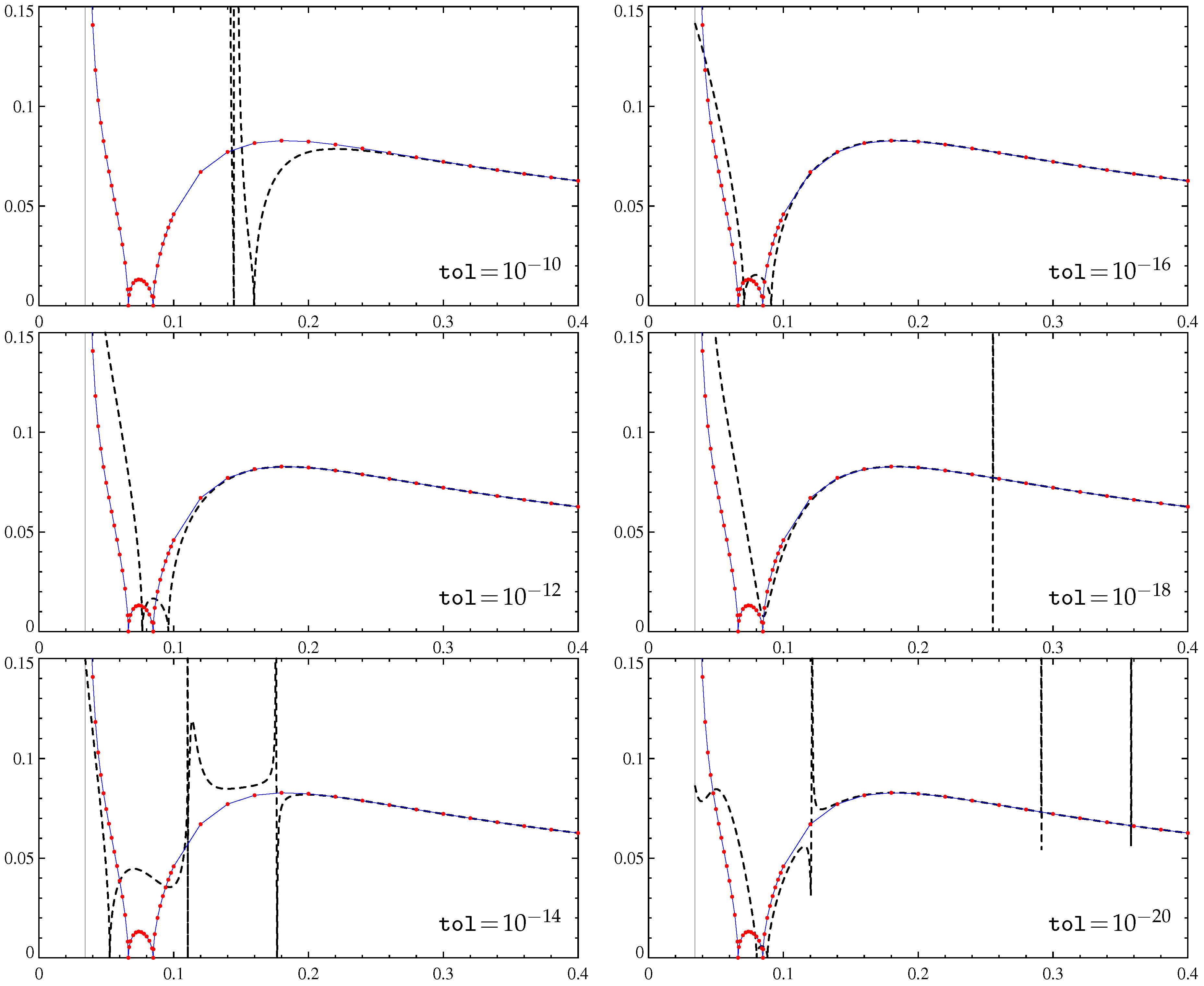
We have tried the algorithm in [35] for a set of $\mathtt{tol}$ values ranging between ${10}^{-10}$ and ${10}^{-20}$ using the MATLAB procedure provided by the authors of [35]. We have computed 65 first coefficients of the power series expansions of the symmetrized $\alpha$-effect tensor entries ${\left({{}^{\mathrm{s}}\mathfrak{A}}_k\right)}_l^{\left(n\right)}$ (which involve only odd powers of $1/\eta$; see Section 3.2) up to order ${\eta }^{-129}$ terms with the spatial resolution of ${64}^3$ Fourier harmonics. The MATLAB procedure has been requested to construct the [63/64] Padé approximants for each entry. The results are shown in Figure 2. We observe that the approximations of the maximum growth rates ${\gamma }_{\alpha }$ are relatively accurate for $\mathtt{tol}={10}^{-12}$ and ${10}^{-16}$ for $\eta \gtrsim 0.1$. This bound is roughly 5 times smaller than the minimal $\eta$ for which the power series for ${{}^{\mathrm{s}}\mathfrak{A}}_k^l$ converge.

Table 2. Order parameter L of the Padé approximants $[2L-1/2L]$ (ratios of polynomials in $1/\eta$) constructed by the algorithm in [35] for six independent entries of the symmetrized $\alpha$-effect tensor ${}^{\mathrm{s}}\mathfrak{A}$.

tol	${{}^{\mathbf{s}}\mathfrak{A}}_1^1$	${{}^{\mathbf{s}}\mathfrak{A}}_1^2$	${{}^{\mathbf{s}}\mathfrak{A}}_1^3$	${{}^{\mathbf{s}}\mathfrak{A}}_2^2$	${{}^{\mathbf{s}}\mathfrak{A}}_2^3$	${{}^{\mathbf{s}}\mathfrak{A}}_3^3$
${10}^{-10}$	5	5	6	5	5	5
${10}^{-12}$	6	6	6	6	6	6
${10}^{-14}$	7	7	8	7	7	7
${10}^{-16}$	8	8	9	8	8	8
${10}^{-18}$	9	8	10	10	9	9
${10}^{-20}$	10	10	11	10	10	10

sheds light on the reasons why the gain is unsatisfactory (for $\eta \ge 0.1$ spectral computations of the $\alpha$-effect, growth rates for individual $\eta$’s are efficient): since the rank decreases, when small in absolute value, singular values are discarded, and the algorithm ends up with very moderate orders $[2L/2L-1]$.

The four remaining panels in Figure 2 reveal the presence of the so-called Froissart doublets in the approximants of some entries. Froissart doublets is a factor of the form $(1/\eta -a)/(1/\eta -\tilde{a})$ in the approximant, where the two constants a and $\tilde{a}$ are close but distinct. Such a factor implies a singular behavior of the approximant for $1/\eta$ close to $\tilde{a}$, not altering its behavior much at distances from $\tilde{a}$ significantly larger than $|a-\tilde{a}|$. Often, such factors are artifacts emerging due to noise in the data. Almost vertical segments of the plots are signatures of the Froissart doublets (see Figure 2). They extend to both positive and negative infinity in the graphs of the approximants, but since (20) are nonlinear functions of the tensor entries, the respective segments of graphs of ${\gamma }_{\alpha }$ may be bounded from below and/or above. (Their detection has proven unexpectedly difficult; in order to reliably show their full range in the vertical direction, we have plotted the approximation step ${10}^{-9}$ along the abscissa.) We thus see that although the algorithm in [35] is supposed to be robust, it is prone to yielding approximants involving Froissart doublets.

3.3.2. Approximation by the Algorithm II

Since we have failed to obtain satisfactory results with the use of the algorithm I in [35], we have also tested the algorithm II in [5]. Quoting from [5], although the equations for the coefficients of the approximant involve a matrix in the Toeplitz form, “experience shows that the equations are frequently close to singular, so that one should not solve them by the methods” relying on this form, “but rather by full LU decomposition. Additionally, it is a good idea to refine the solution by iterative improvement (routine mprove in §2.5)”. This is implemented in their pade procedure. We have used it with one alteration: the routine mprove stops when the discrepancy increases; instead, it has been allowed to make up to 1000 improvement iterations, permitting the discrepancy to temporarily grow and storing the minimum-discrepancy solution obtained in the course of these iterations (however, it has often been forced to stop before the allowed number of iterations has been performed, the iterative process blowing up with an overflow).

Approximate maximum slow-time growth rates (20) of large-scale magnetic modes generated by the $\alpha$-effect have been computed for the same flow again using $[2L-1/2L]$ Padé approximants for the entries ${{}^{\mathrm{s}}\mathfrak{A}}_l^k\left(\eta \right)$. They are compared in Figure 3 for increasing orders L with the actual maximum growth rates obtained by direct computation of the fields ${\mathbf{s}}_k$ using spectral methods for individual molecular diffusivities $\eta$.

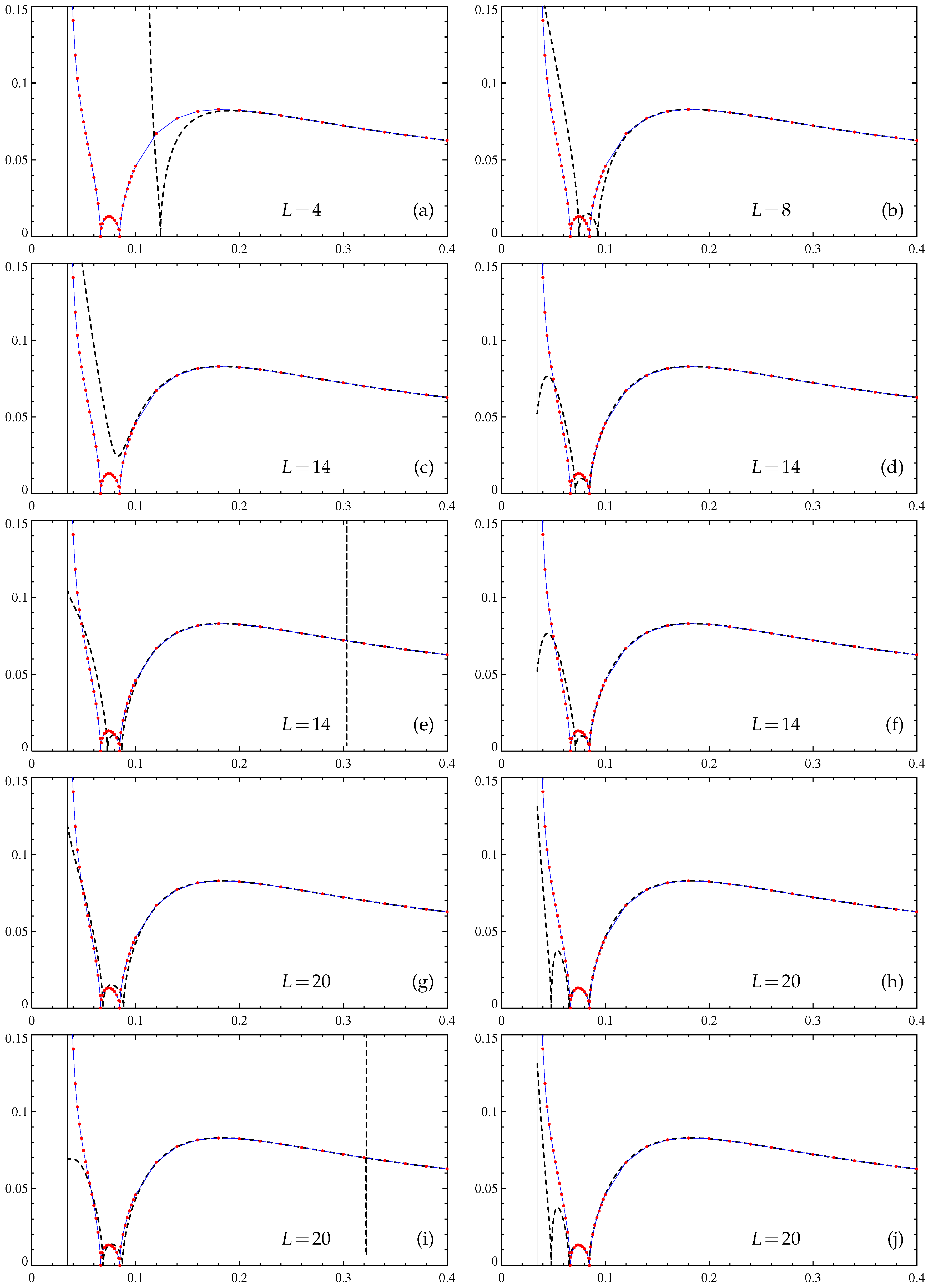
Four Padé approximants $[2L-1/2L]$ of the entries of the $\alpha$-effect tensor have been constructed for each considered L, using the resolution of ${64}^3$ or ${512}^3$ Fourier harmonics and running our code with the double (real*8) or extended quadruple (real*16) precision of the floating-point number arithmetics. In computers built around Intel and compatible processors, the former is standard, and the latter is not supported by hardware but is software-emulated; however, many compilers do not require modifying the Fortran source code to use it, all of the floating-point data and computations can be readily promoted to the real*16 precision by using the appropriate compiler option such as −r16. Higher precision and resolution has been expected to improve the accuracy of the coefficients of the approximants, to augment the orders of the approximants beyond those produced by the algorithm in [35], and to increase the $\eta$ interval, where the growth rate values determined for the approximated $\alpha$-effect tensor are close to the actual growth rates.

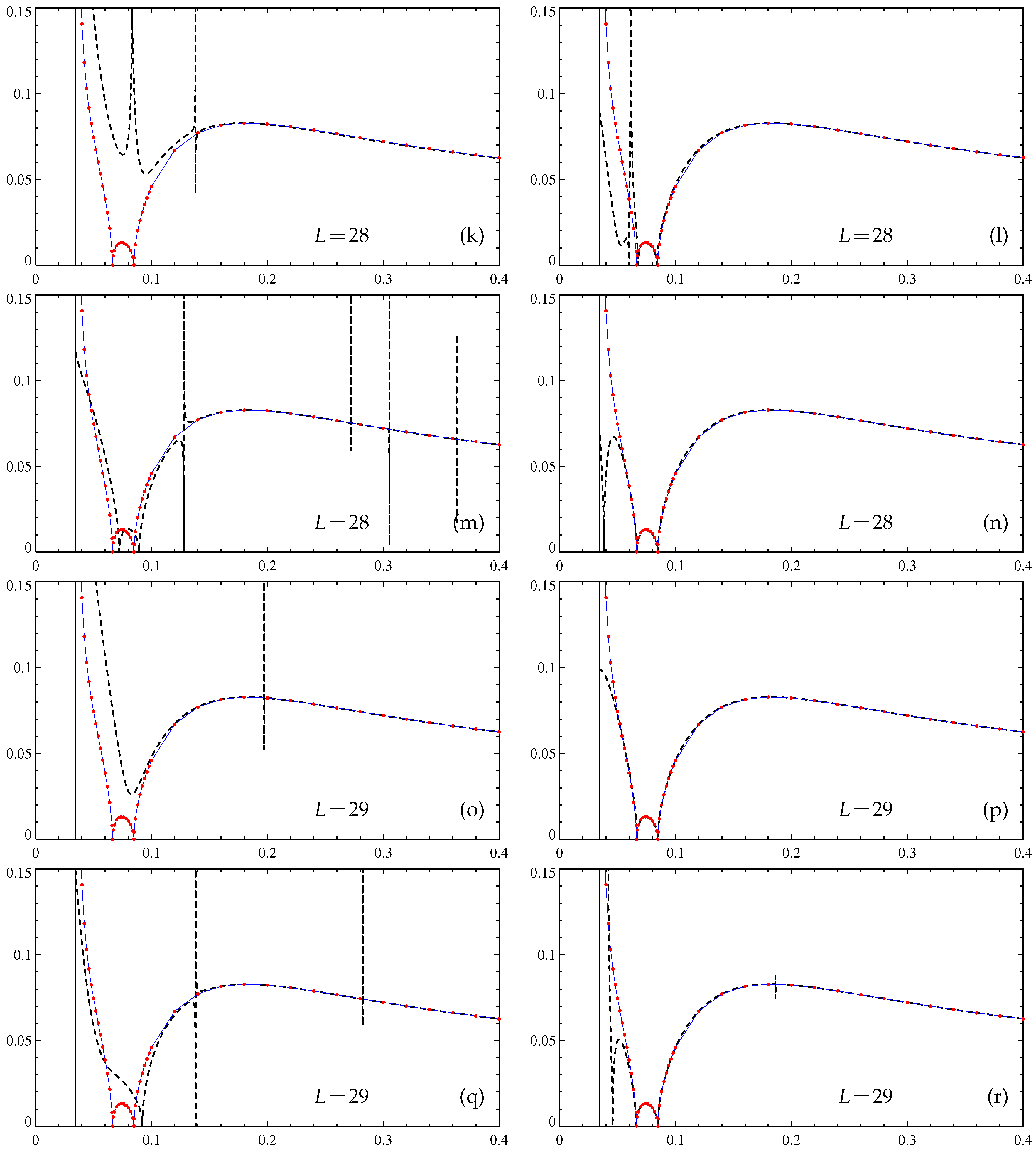
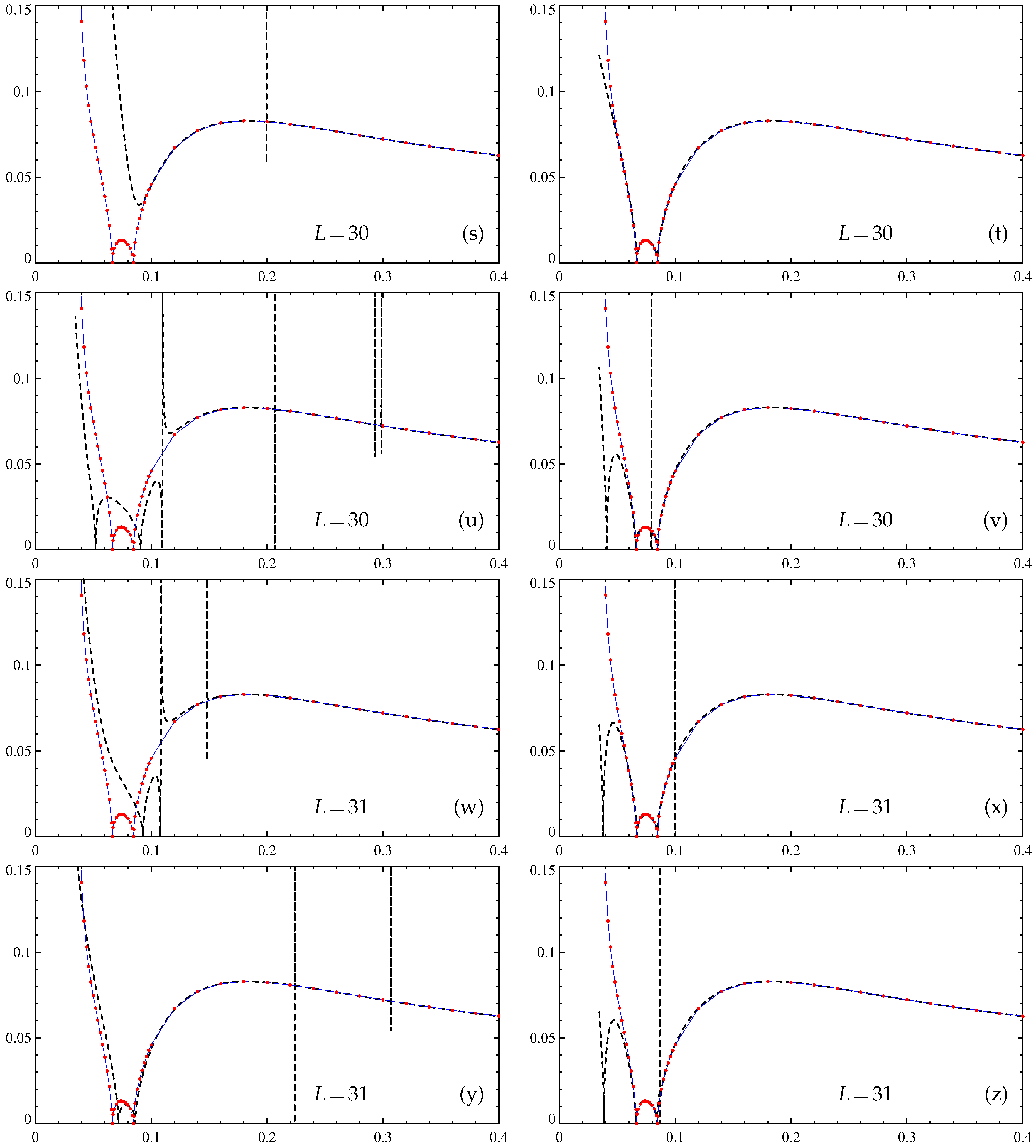
In Figure 3, we show the resultant approximations of ${\gamma }_{\alpha }$ for $L=4$, 8, 14, 20, and 28 to 31. The four graphs for $L=4$ are visually indistinguishable, and we show only one of them; the same holds true for $L=8$. For $L=14$ and 20, the plots of the approximated ${\gamma }_{\alpha }$, computed with quadruple precision for the two spatial resolutions, also visually coincide (Figure 3d,f,h,j), but this is wrong for the respective double precision approximations. For higher L, all four plots are visually distinct. The quadruple precision approximations are plagued much less by the Froissart doublets (and never involve multiple occurrences of the doublets) than the double precision ones. Three high-L quadruple precision approximations are reasonably accurate for $L=28$ and the ${512}^3$ resolution for $\eta \ge 0.055$ (Figure 3n), for $L=29$ and the ${64}^3$ resolution for $\eta \ge 0.05$ (Figure 3p), and for $L=30$ and the ${64}^3$ resolution for $\eta \ge 0.05$ (Figure 3t). Thus, the left end of the interval of validity of Padé approximations has decreased roughly twice compared to that obtained by the algorithm in [35]. All other quadruple-precision approximations for $L\ge 29$ (Figure 3r,v,x,z) can also give reasonable accuracy for $\eta \gtrsim 0.06÷0.07$ upon removal of Froissart doublets from the affected approximants of ${{}^{\mathrm{s}}\mathfrak{A}}_l^k$.

These results suggest that Padé approximants are useful for representing the functional dependence of the slow-time growth rates (20) of large-scale magnetic modes generated by the $\alpha$-effect for fairly low magnetic molecular diffusivities. However, for the construction of Padé approximants, accurate enough to serve small $\eta$, the quadruple precision arithmetics must be used, and hence run times become comparable to those of direct computation of the growth rates at individual $\eta$s (note that real*16 computations are typically ten times slower than real*8 ones). Therefore, another strategy is perhaps also sensible: in computations for an individual $\eta$, to use relatively low-order, not very precise Padé approximants for neutral modes ${\mathbf{s}}_k$ (constructed, for instance, at each point in space or for each Fourier harmonics within the employed resolution) as the initial data for further refinement by the usual iterative methods.

4. Computation of the Magnetic Eddy Diffusivity Tensor

As discussed in Section 2, an important class are parity-invariant flows. This symmetry is compatible with the equations of fluid dynamics (the Navier–Stokes or Euler equations) provided the forcing has the same property. For such a flow, the domain of the operator of magnetic induction $\mathfrak{L}$ splits into the subspaces of parity-invariant fields (such that $\mathbf{f}(-\mathbf{x})=-\mathbf{f}\left(\mathbf{x}\right)$) and of parity-anti-invariant ones (such that $\mathbf{f}(-\mathbf{x})=\mathbf{f}\left(\mathbf{x}\right)$). Solutions to the auxiliary problems (14), ${\mathbf{s}}_k\left(\mathbf{x}\right)$, are therefore parity-anti-invariant. This implies $\mathfrak{A}=0$ (see (17)), i.e., no $\alpha$-effect acts in such flows, and hence ${\lambda }_1=0$.

4.1. The Multiscale Formalism Revealing the Magnetic Eddy Diffusivity

By (15),

$${\mathbf{b}}_1=\sum _{k=1}^3\sum _{m=1}^3\frac{\partial {〈{\mathbf{b}}_0〉}_k}{\partial X_m}{\mathbf{g}}_{mk},$$

where the small-scale zero-mean (non-solenoidal!) fields ${\mathbf{g}}_{mk}\left(\mathbf{x}\right)$ solve nine auxiliary problems of type II:

$$\mathfrak{L}{\mathbf{g}}_{mk}=-2\eta \frac{\partial {\mathbf{s}}_k}{\partial x_m}-{\mathbf{e}}_m\times (\mathbf{v}\times {\mathbf{s}}_k).$$

(28)

For parity-invariant $\mathbf{v}$, ${\mathbf{g}}_{mk}\left(\mathbf{x}\right)$ are also parity-invariant. Moreover, ${\mathbf{b}}_n$ are parity-anti-invariant for all even n and parity-invariant for odd n [17] in the expansion (12), and no odd powers of $\epsilon$ enter the series (13) for the eigenvalue $\lambda$.

Averaging the third (order ${\epsilon }^2$) equation in the hierarchy yields

$$\eta {\nabla }_{\mathbf{X}}^2〈{\mathbf{b}}_0〉+{\nabla }_{\mathbf{X}}\times \sum _{k=1}^3\sum _{m=1}^3{\mathfrak{D}}_{mk}\frac{\partial {〈{\mathbf{b}}_0〉}_k}{\partial X_m}={\lambda }_2〈{\mathbf{b}}_0〉,$$

(29)

where

$${\mathfrak{D}}_{mk}=〈\mathbf{v}\times {\mathbf{g}}_{mk}〉$$

(30)

is the so-called tensor of magnetic eddy diffusivity correction. Again assuming that the mean field $〈{\mathbf{b}}_0〉$ is a Fourier harmonic (18), we find [20]

$${\lambda }_{2_{\pm }}\left(\mathbf{q}\right)=-\eta -\frac{1}{2}\sum _{j,l,n}(D_n^l-D_l^n)q_j\pm \sqrt{d},$$

(31)

$$d=\sum _{j,l,n}\left(({\left({{}^{\mathrm{s}}D}_n^l\right)}^2-{{}^{\mathrm{s}}D}_l^l{{}^{\mathrm{s}}D}_n^n)q_j^2-2q_j{q}_n({{}^{\mathrm{s}}D}_n^l{{}^{\mathrm{s}}D}_j^l-{{}^{\mathrm{s}}D}_l^l{{}^{\mathrm{s}}D}_j^n)\right),$$

(32)

where both sums are over even permutations of indices 1, 2, and 3 (i.e., $(j,l,n)$ are combinations (1,2,3), (2,3,1), and (3,1,2)), and it is denoted

$$D_n^l=\sum _m{\mathfrak{D}}_{mn}^l{q}_m,{{}^{\mathrm{s}}D}_n^l=(D_n^l+D_l^n)/2.$$

(33)

The minimum

$${\eta }_{\mathrm{eddy}}\equiv \underset{\left|\mathbf{q}\right|=1}{min}(-\mathrm{Re}{\lambda }_{2_{\pm }}\left(\mathbf{q}\right))$$

(34)

is called the minimum magnetic eddy diffusivity. When it is negative, the interaction of the fluctuating small-scale velocity and magnetic field is capable of generating large-scale magnetic fields. For this reason, this quantity is of prime interest in large-scale dynamo theory.

Expression (30) can be transformed into

$${\mathfrak{D}}_{mk}^l=〈{\mathbf{Z}}_l·\left(2\eta \frac{\partial {\mathbf{s}}_k}{\partial x_m}+{\mathbf{e}}_m\times (\mathbf{v}\times {\mathbf{s}}_k)\right)〉,$$

(35)

where ${\mathbf{Z}}_l$ are zero-mean solutions to three auxiliary problems for the adjoint operator:

$${\mathfrak{L}}^{*}{\mathbf{Z}}_l=\mathbf{v}\times {\mathbf{e}}_l,$$

(36)

and ${\mathfrak{L}}^{*}:\mathbf{z}\mapsto \eta {\nabla }^2\mathbf{z}-\{\mathbf{v}\times (\nabla \times \mathbf{z})\}$ is the operator adjoint to $\mathfrak{L}$ acting in the space of zero-mean space-periodic fields.

4.2. Padé Approximation

Relation (30) suggests constructing expansions of the solutions to the auxiliary problems in the inverse molecular diffusivity, (21), and

$${\mathbf{g}}_{mk}=\sum _{n=1}^{\infty }{\mathbf{g}}_{mk}^{\left(n\right)}{\eta }^{-n}.$$

(37)

Dividing (28) by $\eta$ yields

$${\nabla }^2{\mathbf{g}}_{mk}=-{\eta }^{-1}\nabla \times (\mathbf{v}\times {\mathbf{g}}_{mk})-2\frac{\partial {\mathbf{s}}_k}{\partial x_m}-{\eta }^{-1}{\mathbf{e}}_m\times (\mathbf{v}\times {\mathbf{s}}_k),$$

whereby

$${\mathbf{g}}_{mk}^{\left(1\right)}=-{\nabla }^{-2}\left(2\frac{\partial {\mathbf{s}}_k^{\left(1\right)}}{\partial x_m}+{\mathbf{e}}_m\times (\mathbf{v}\times {\mathbf{e}}_k)\right),$$

(38)

$${\mathbf{g}}_{mk}^{\left(n\right)}=-{\nabla }^{-2}\left(\nabla \times (\mathbf{v}\times {\mathbf{g}}_{mk}^{(n-1)})+2\frac{\partial {\mathbf{s}}_k^{\left(n\right)}}{\partial x_m}+{\mathbf{e}}_m\times (\mathbf{v}\times {\mathbf{s}}_k^{(n-1)})\right)\mathrm{for}n>1.$$

(39)

Clearly, the flow being parity-invariant, all ${\mathbf{s}}_k^{\left(n\right)}$ are parity-anti-invariant and all ${\mathbf{g}}_{mk}^{\left(n\right)}$, parity-invariant. By (30) and (37),

$${\mathfrak{D}}_{mk}=\sum _{n=1}^{\infty }{\mathfrak{D}}_{mk}^{\left(n\right)}{\eta }^{-n},{\mathfrak{D}}_{mk}^{\left(n\right)}=〈\mathbf{v}\times {\mathbf{g}}_{mk}^{\left(n\right)}〉.$$

(40)

Thus, algorithm I consists of the following steps:

•

find the fields ${\mathbf{s}}_k^{\left(n\right)}$ employing (22);

•

find the fields ${\mathbf{g}}_{mk}^{\left(n\right)}$ employing (38) and (39);

•

calculate the coefficients ${\mathfrak{D}}_{mk}^{\left(n\right)}$ employing (40).

Expressions (40) reveal symmetry properties of coefficients in the eddy diffusivity tensor expansion (similar to those of the coefficients of the $\alpha$-effect tensor expansion). Eddy diffusivity tensor for the reverse flow $-\mathbf{v}$ is related to that of the flow $\mathbf{v}$ by the relations ${\left({\mathfrak{D}}_{ml}^{-}\right)}_k=-{\mathfrak{D}}_{mk}^l$ [19]. By (38) and (39), ${\mathbf{g}}_{mk}^{\left(n\right)}={(-1)}^n{\left({\mathbf{g}}_{mk}^{-}\right)}^{\left(n\right)}$. Thus, identities, analogous to those used in the case of the $\alpha$-effect tensor, reveal that for each fixed m, the coefficients ${\left({\mathfrak{D}}_{mk}^l\right)}^{\left(n\right)}$ in the series (40) are symmetric $3\times 3$ matrices for even n, and antisymmetric ones for odd n. This implies that the symmetrized matrix ${}^{\mathrm{s}}\mathbf{D}$ (33), determining the discriminant d (32), is expanded in even powers of $1/\eta$, and the antisymmetric one $\mathbf{D}-{}^{\mathrm{s}}\mathbf{D}$, determining the common part of ${\lambda }_{2_{\pm }}\left(\mathbf{q}\right)$ (31), in odd powers.

It is simple to show that, like in the case of $\alpha$-effect dynamos, for a given flow $\mathbf{v}$, the radius of convergence of all of the series (37) and (40) (regarded as functions of $1/\eta$) is generically equal to $1/{max}_i\left|{\mu }_i\right|$, where ${\mu }_i$ are eigenvalues of the compact operator $\mathfrak{M}$ (23); convergence of the series is guaranteed for $\eta >{max}_i\left|{\mu }_i\right|$.

An alternative form of the eddy diffusivity tensor can be exploited. Comparing (14) and (36), we find

$${\mathbf{e}}_l+\nabla \times {\mathbf{Z}}_l={\mathbf{s}}_l^{-}\Rightarrow {\mathbf{Z}}_l={\eta }^{-1}{\nabla }^{-2}(\mathbf{v}\times {\mathbf{s}}_l^{-}),$$

(41)

where the superscript minus denotes objects pertinent to the reverse flow $-\mathbf{v}$ (see (25)). Using (41) to eliminate ${\mathbf{s}}_k$ in (35) yields [19]

$${\mathfrak{D}}_{mk}^l=\eta 〈{\mathbf{Z}}_l·\left(2\nabla \times \frac{\partial {\mathbf{Z}}_k^{-}}{\partial x_m}-{\mathbf{e}}_m\times {\nabla }^2{\mathbf{Z}}_k^{-}\right)〉.$$

(42)

By (41), all ${\mathbf{Z}}_l$ are parity-invariant, and hence (36) is equivalent to

$${\nabla }^2{\mathbf{Z}}_l={\eta }^{-1}(\mathbf{v}\times ({\mathbf{e}}_l+\nabla \times {\mathbf{Z}}_l)),$$

which implies a power series expansion

$${\mathbf{Z}}_l=\sum _{n=1}^{\infty }{\mathbf{Z}}_l^{\left(n\right)}{\eta }^{-n},$$

(43)

where the coefficients satisfy recurrence relations

$${\mathbf{Z}}_l^{\left(1\right)}={\nabla }^{-2}(\mathbf{v}\times {\mathbf{e}}_l),{\mathbf{Z}}_l^{\left(n\right)}={\nabla }^{-2}(\mathbf{v}\times (\nabla \times {\mathbf{Z}}_l^{(n-1)}))\mathrm{for}n>1.$$

(44)

By linearity of (44) in $\mathbf{v}$, the coefficients of such an expansion for the reverse flow are linked:

$${\left({\mathbf{Z}}_l^{-}\right)}^{\left(n\right)}={(-1)}^n{\mathbf{Z}}_l^{\left(n\right)}.$$

This implies algorithm II for calculation of ${\left({\mathfrak{D}}_{mk}^l\right)}^{\left(n\right)}$ based on (42):

• find the fields ${\mathbf{Z}}_l^{\left(n\right)}$ applying (44);

• for $n\ge 1$ calculate

$${\left({\mathfrak{D}}_{mk}^l\right)}^{\left(n\right)}=\sum _{j=1}^n{(-1)}^j〈{\mathbf{Z}}_l^{(n+1-j)}·\left(2\nabla \times \frac{\partial {\mathbf{Z}}_k^{\left(j\right)}}{\partial x_m}-{\mathbf{e}}_m\times {\nabla }^2{\mathbf{Z}}_k^{\left(j\right)}\right)〉.$$

(45)

Using (41), it is straightforward, albeit tedious, to transform (42) into

$${\mathfrak{D}}_{mk}^l=\eta {〈\left\{{\mathbf{s}}_l^{-}\right\}\times \left\{{\mathbf{s}}_k\right\}-\left\{{\mathbf{s}}_k\right\}\nabla ·{\mathbf{Z}}_l+\left\{{\mathbf{s}}_l^{-}\right\}\nabla ·{\mathbf{Z}}_k^{-}〉}_m.$$

(46)

Relations (41) imply

$$\nabla \times {\mathbf{Z}}_l^{\left(n\right)}={(-1)}^n{\mathbf{s}}_l^{\left(n\right)},{\mathbf{Z}}_l^{\left(n\right)}={(-1)}^{n-1}{\nabla }^{-2}(\mathbf{v}\times {\mathbf{s}}_l^{(n-1)})\mathrm{for}n\ge 1.$$

(47)

Thus, the coefficients in the expansion (40) have the entries

$${\left({\mathfrak{D}}_{mk}^l\right)}^{\left(n\right)}=\sum _{j=1}^n{〈{(-1)}^j{\mathbf{s}}_l^{\left(j\right)}\times {\mathbf{s}}_k^{(n+1-j)}-{\mathbf{s}}_k^{(n+1-j)}\nabla ·{\mathbf{Z}}_l^{\left(j\right)}-{(-1)}^n{\mathbf{s}}_l^{(n+1-j)}\nabla ·{\mathbf{Z}}_k^{\left(j\right)}〉}_m.$$

(48)

Algorithm III consists of the following steps:

•

determine coefficients in the expansion of the neutral magnetic modes ${\mathbf{s}}_k$ applying recurrence relations (22);

•

in the course of these calculations, determine coefficients in the expansion of $\nabla ·{\mathbf{Z}}_l$ using (47);

•

calculate the coefficients ${\left({\mathfrak{D}}_{mk}^l\right)}^{\left(n\right)}$ applying (48).

If the flow $\mathbf{v}$ involves a small number of Fourier harmonics, it is unclear a priori which of the three algorithms is more efficient. Algorithm I involves the computation of two sets of coefficients, for ${\mathbf{s}}_k$ and ${\mathbf{g}}_{mk}$, algorithm II, only of the set of coefficients for ${\mathbf{Z}}_l$, and algorithm III is an intermediate case involving two sets of coefficients, for ${\mathbf{s}}_k$ and $\nabla ·{\mathbf{Z}}_l$. However, the calculation of the n-term sums (45) and (48) in algorithms II and III, respectively, is computer-intensive.

4.3. Numerical Results

For numerical experimentation, we have applied two types of flows: the so-called cosine flows introduced in [20], and their curls, considered in [21]. They are of interest in that the latter have a point-wise zero vorticity (kinematic) helicity, and the former have a point-wise zero velocity helicity, but nevertheless they are capable of both small- and large-scale magnetic field generation (see ibid.). Involving a small number of trigonometric functions, they are particularly useful for calculating the Taylor series coefficients (40).

The cosine flows are defined as follows:

$$\begin{array}{cc}\hfill v_1& =\beta n(b_{1}sin\left(\mathbf{a}·\mathbf{x}\right)+a_{1}sin\left(\mathbf{b}·\mathbf{x}\right))cosn{x}_3,\hfill \\ \hfill v_2& =\beta n(b_{2}sin\left(\mathbf{a}·\mathbf{x}\right)+a_{2}sin\left(\mathbf{b}·\mathbf{x}\right))cosn{x}_3,\hfill \\ \hfill v_3& =-\beta \left(\mathbf{a}·\mathbf{b}\right)(cos\left(\mathbf{a}·\mathbf{x}\right)+cos\left(\mathbf{b}·\mathbf{x}\right))sinn{x}_3.\hfill \end{array}$$

(49)

Here, $\mathit{a}=(a_1,a_2,0)$ and $\mathbf{b}=(b_1,b_2,0)$ are constant horizontal vectors, and

$$\beta =2(n^2{\left(\right|\mathbf{a}|}^2+{\left|\mathbf{b}\right|}^2{)+2{\left(\mathbf{a}·\mathbf{b}\right)}^2)}^{-1/2},$$

so that the r.m.s. flow velocity is unity.

Because of many symmetries of the cosine flows, all entries of the eddy diffusivity tensor $\mathfrak{D}$ vanish, except for five pairs (see [20]):

$${\mathfrak{D}}_{31}^2=-{\mathfrak{D}}_{32}^1,{\mathfrak{D}}_{12}^3=-{\mathfrak{D}}_{13}^2,{\mathfrak{D}}_{23}^1=-{\mathfrak{D}}_{21}^3,{\mathfrak{D}}_{22}^3=-{\mathfrak{D}}_{23}^2,{\mathfrak{D}}_{13}^1=-{\mathfrak{D}}_{11}^3.$$

Consequently, the minimum eddy diffusivity (34) takes a simple form:

$${\eta }_{\mathrm{eddy}}=\eta -max\left({\mathfrak{D}}_{31}^2,\frac{1}{2}\left({\mathfrak{D}}_{12}^3+{\mathfrak{D}}_{23}^1+\sqrt{{({\mathfrak{D}}_{12}^3-{\mathfrak{D}}_{23}^1)}^2+{({\mathfrak{D}}_{22}^3+{\mathfrak{D}}_{13}^1)}^2}\right)\right).$$

(50)

We have considered the particular sample flow for

$$\mathbf{a}=(1,0,0),\mathbf{b}=(1,1,0),n=1$$

(51)

and used Mathematica again to implement algorithm I: we have calculated exactly the coefficients of the expansions (21) and (37) of solutions to the auxiliary problems (14) and (28) using the recurrence relations (22) and (38) and (39), and of the coefficients ${\mathfrak{D}}_{mk}^{\left(n\right)}$ of the series (40) up to order ${\eta }^{-49}$. The precise coefficients ${\mathbf{s}}_k^{\left(49\right)}$ and ${\mathbf{g}}_{mk}^{\left(49\right)}$ require about 2 Gbytes of memory for storage (in the ASCII form). For the flow (49), the coefficients ${\mathfrak{D}}_{mk}^{\left(n\right)}$ turn out to be rational; in the ASCII form, the vectors ${\mathfrak{D}}_{mk}^{\left(49\right)}$ occupy 10 to 20 Kbytes of memory.

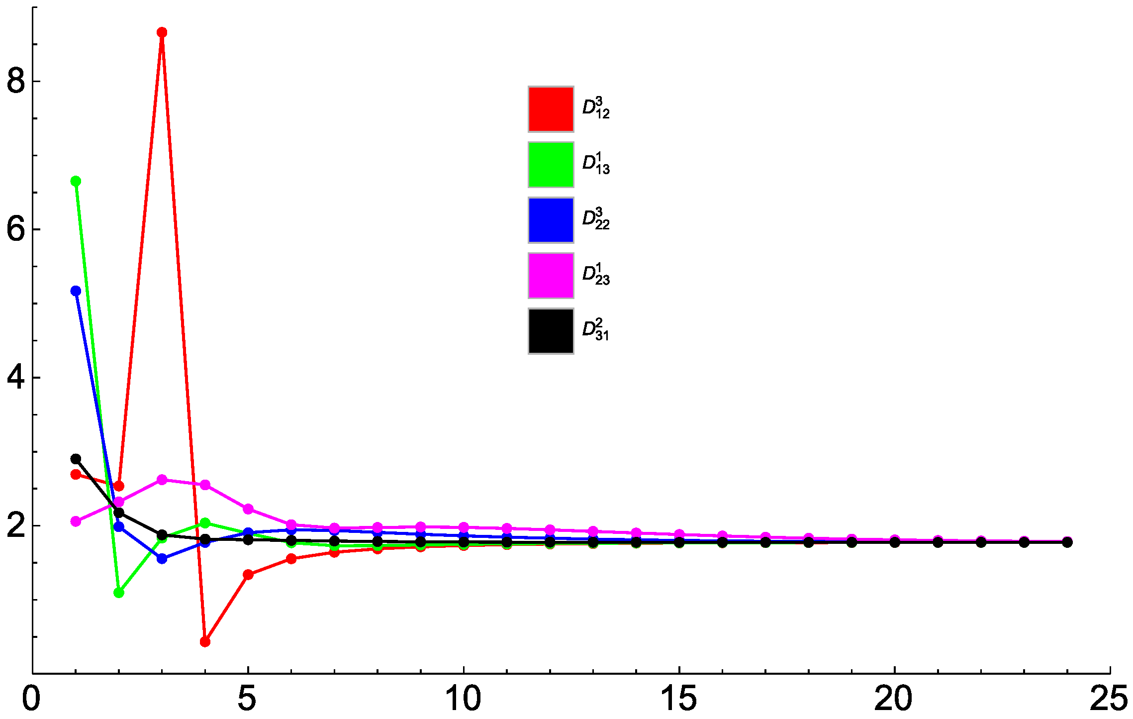
Figure 4 shows the sequence of the ratios $|{\left({\mathfrak{D}}_{mk}^l\right)}^{(2n-1)}/{\left({\mathfrak{D}}_{mk}^l\right)}^{(2n+1)}{|}^{1/2}$ for five independent entries. The limit of this sequence for $n\to \infty$ is equal to the radius of convergence of the series (40) (regarded as a function of $1/\eta$) for the respective entry (note that due to the antisymmetry in l and k, the entries involve only odd powers of $1/\eta$). The figure demonstrates that the series for the five entries have the same radius of convergence and converge for $\eta \gtrsim 0.5.$

Because precise Mathematica calculations require considerable computer resources, we have not considered high-order Padé approximants. The amount of calculations reduces if meromorphic functions

$$q_1={\mathfrak{D}}_{31}^2,q_2=({\mathfrak{D}}_{12}^3+{\mathfrak{D}}_{23}^1)/2,q_3=({({\mathfrak{D}}_{12}^3-{\mathfrak{D}}_{23}^1)}^2+{({\mathfrak{D}}_{22}^3+{\mathfrak{D}}_{13}^1)}^2)/4$$

(52)

are approximated only, in terms of which (see (50))

$${\eta }_{\mathrm{eddy}}=\eta -max(q_1,q_2+\sqrt{q_3}).$$

(53)

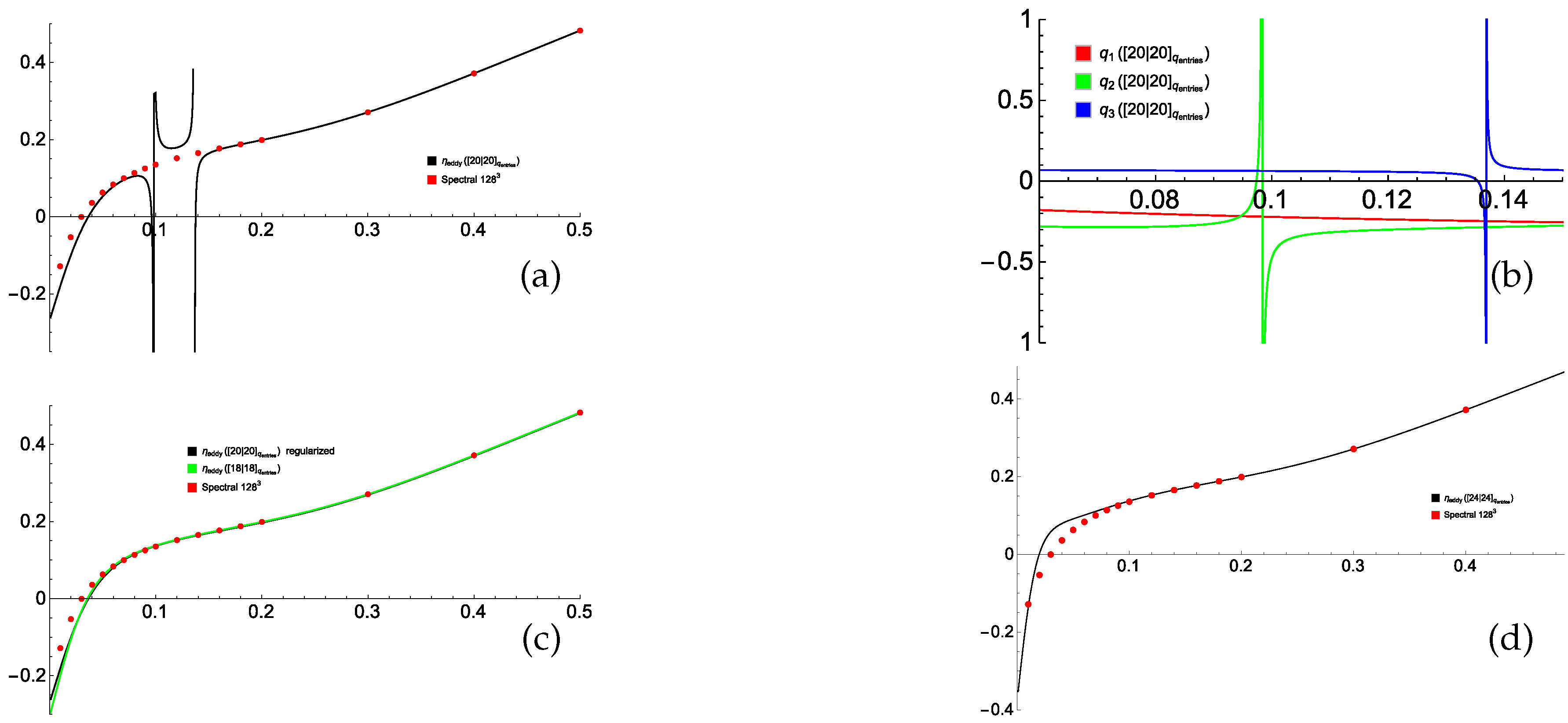
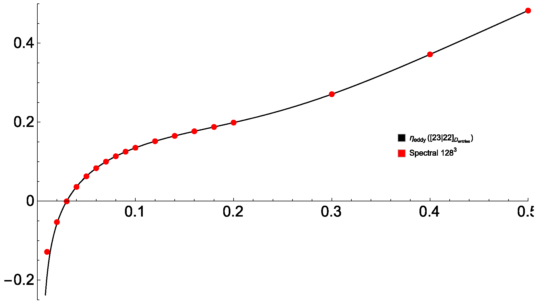
The poor quality of the resultant approximation (see Figure 5a) is due to the presence of two Froissart doublets in the approximants of $q_2$ and $q_3$ (Figure 5b). Gaps are present in the plot in Figure 5a, where the approximant of $q_3$ becomes negative due to its singular behavior, and thus the square root in (53) cannot be extracted. Upon factoring the doublets out (which is simple in Mathematica) in the two plagued approximants, the quality of the approximation becomes very similar to that obtained by using [18/18] approximants of $q_i$ (see Figure 5c). Increasing the orders to [24/24] does not significantly improve the approximated ${\eta }_{\mathrm{eddy}}$ (see Figure 5d). A better approximation is obtained if the elements of the eddy diffusivity tensor $\mathfrak{D}$ are Padé-approximated individually (see Figure 6); this gives reasonably accurate values of ${\eta }_{\mathrm{eddy}}$ for $\eta \gtrsim 0.02$, which is roughly 25 times larger than the minimum $\eta$, for which the power series in $1/\eta$ for the fields ${\mathbf{s}}_k$ and ${\mathbf{g}}_{mk}$, as well as the elements of the tensor $\mathfrak{D}$, are convergent.

Upon shifting by a quarter of the period in the vertical coordinate $x_3$, the curl of (49) takes the form

$$\begin{array}{cc}\hfill v_1=& \beta \left((\left(\mathbf{a}·\mathbf{b}\right)a_2+n^2{b}_2)sin\left(\mathbf{a}·\mathbf{x}\right)+(\left(\mathbf{a}·\mathbf{b}\right)b_2+n^2{a}_2)sin\left(\mathbf{b}·\mathbf{x}\right)\right)cosn{x}_3,\hfill \\ \hfill v_2=& -\beta \left((\left(\mathbf{a}·\mathbf{b}\right)a_1+n^2{b}_1)sin\left(\mathbf{a}·\mathbf{x}\right)+(\left(\mathbf{a}·\mathbf{b}\right)b_1+n^2{a}_1)sin\left(\mathbf{b}·\mathbf{x}\right)\right)cosn{x}_3,\hfill \\ \hfill v_3=& \beta n(a_2{b}_1-a_1{b}_2)(cos\left(\mathbf{a}·\mathbf{x}\right)-cos\left(\mathbf{b}·\mathbf{x}\right))sinn{x}_3,\hfill \end{array}$$

(54)

where we now assume the normalizing factor

$$\beta =2{\left((n^4+{\left(\mathbf{a}·\mathbf{b}\right)}^2){\left(\right|\mathbf{a}|}^2+{\left|\mathbf{b}\right|}^2)+2n^2{(\left(\mathbf{a}·\mathbf{b}\right)}^2+{\left|\mathbf{a}\right|}^2{\left|\mathbf{b}\right|}^2)\right)}^{-1/2},$$

for which the r.m.s. flow velocity is again 1. Since this flow possesses all the symmetries of (49), the expression (50) for the minimum eddy diffusivity still applies.

Following algorithm II, for a sample flow (54) for

$$\mathbf{a}=(0,1,0),\mathbf{b}=(2,2,0),n=1,$$

(55)

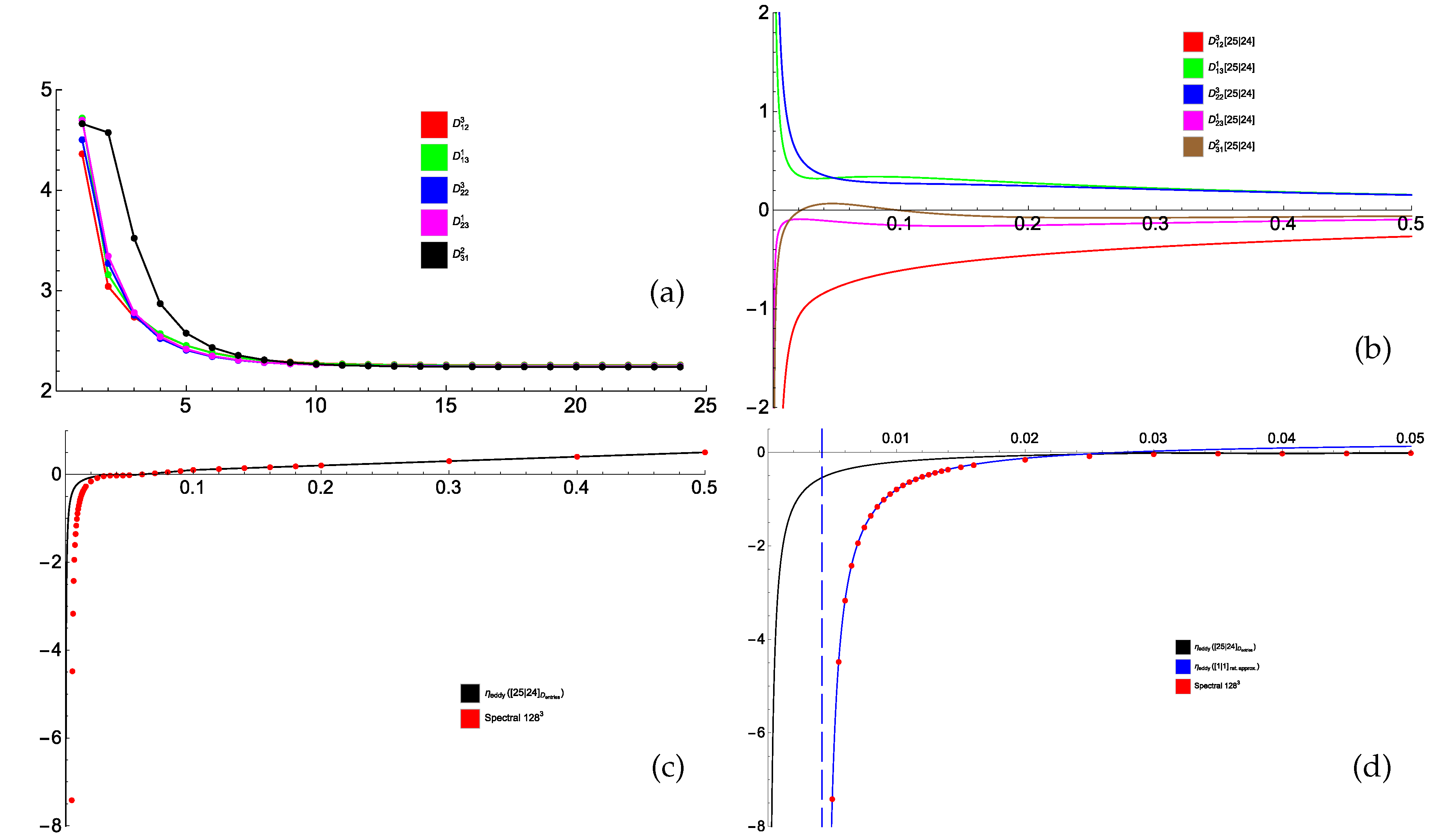
we have calculated with Mathematica 49 coefficients ${\mathfrak{D}}_{mk}^{\left(n\right)}$ of the series (40) up to order ${\eta }^{-49}$. The graph of the ratios $|{\left({\mathfrak{D}}_{mk}^l\right)}^{(2n-1)}/{\left({\mathfrak{D}}_{mk}^l\right)}^{(2n+1)}{|}^{1/2}$ for the five independent entries (see Figure 7a) of the eddy diffusivity tensor shows that the series (40) converge for $\eta \gtrsim 2.2$. The highest-order (for this set of coefficients) [25/24] approximants of the entries are free of Froissart doublets (see Figure 7b). They yield a satisfactory approximation of dependence on $\eta$ of the minimum magnetic eddy diffusivity for $\eta \gtrsim 0.03$, which is roughly 70 times smaller than the bound obtained for convergence of the Taylor series (40) for ${\mathfrak{D}}_{mk}^l$ (see Figure 7c,d). However, their fidelity is insufficient to reproduce the singularity of the minimum eddy diffusivity observed in Figure 7c,d.

The symmetries of the flow (54), (55) imply that the neutral modes ${\mathbf{s}}_k$ reside in invariant subspaces of the magnetic induction operator, which can be categorized in terms of the Fourier harmonics ${\mathbf{b}}_{\mathbf{n}}{\mathrm{e}}^{\mathrm{i}\mathbf{n}·\mathbf{x}}$, comprising the Fourier series for ${\mathbf{s}}_k$ (by virtue of the mode periodicity, the wave vectors $\mathbf{n}$ have integer components). Only the harmonics that have the following properties enter the Fourier series for ${\mathbf{s}}_k$:

• ${\mathbf{b}}_{\mathbf{n}}={\mathbf{b}}_{-\mathbf{n}}$ are real;
• the numbers $n_1$ and $n_1/2+n_2+n_3$ are even;
• ${\mathbf{s}}_1$ and ${\mathbf{s}}_2$ are symmetric in $x_3$ (i.e., $b_{\mathbf{n}}^1=b_{{\mathbf{n}}^{*}}^1,b_{\mathbf{n}}^2=b_{{\mathbf{n}}^{*}}^2,b_{\mathbf{n}}^3=-b_{{\mathbf{n}}^{*}}^3$), and ${\mathbf{s}}_3$ is antisymmetric in $x_3$ (i.e., $b_{\mathbf{n}}^1=-b_{{\mathbf{n}}^{*}}^1,b_{\mathbf{n}}^2=-b_{{\mathbf{n}}^{*}}^2,b_{\mathbf{n}}^3=b_{{\mathbf{n}}^{*}}^3$), where ${\mathbf{n}}^{*}=(n_1,n_2,-n_3)$.

We have checked that for $\eta >{\eta }_{\mathrm{cr}}=0.00420516$, small-scale modes from the subspace, where ${\mathbf{s}}_1$ and ${\mathbf{s}}_2$ are located, are not generated, but at $\eta ={\eta }_{\mathrm{cr}}$ the small-scale generation starts in the subspace, where ${\mathbf{s}}_3$ resides. It is known [20,21,23] that the point of the onset of the small-scale generation is typically associated with a singularity of the $\alpha$-effect or eddy diffusivity tensors; this is the case for the flow under consideration. In Figure 7d, we observe that the least-squares fit by a hyperbola through 20 computed values of minimum eddy diffusivity at equispaced points in the interval $0.0045\le \eta \le 0.014$ is very accurate (only 19 points out of the 20 are shown; for the smallest $\eta =0.0045$, eddy diffusivity –20.217501, also well approximated by the hyperbola, is out of the vertical range of Figure 7d). The hyperbolic fit yields the location of the singularity at $\eta =0.0041988$ (the vertical asymptote is shown by a dashed line in Figure 7d), which is very close to the point of the onset of the small-scale generation ${\eta }_{\mathrm{cr}}=0.00420516$ computed by spectral methods; the hyperbola through the three smallest $\eta$ from this interval yields a closer value 0.00420233.

5. Conclusions

We have tested Padé approximants of the $\alpha$-effect and eddy diffusivity tensors, responsible for generation of large-scale fields, as functions of the respective molecular diffusivity: the viscosity $\nu$ when hydrodynamic perturbations are studied, and the magnetic diffusivity $\eta$ when the kinematic dynamo problem is under scrutiny. We have tried different computational tools: Fortran codes relying on floating point arithmetics and Mathematica for symbolic and arbitrary precision calculations. A relatively high (several dozens) order of Padé approximants is needed to obtain a reasonable accuracy of approximation of the tensor entries. For this, a high precision of computations (in particular, the quadruple precision in Fortran) has proved indispensable. For our sample flows, the Padé-approximated tensors yield large-scale magnetic field growth rates to satisfactory accuracy for $\eta$, several dozen times smaller than those for which power series in the inverse molecular diffusivity converge, for both large-scale generating mechanisms (the $\alpha$-effect and negative magnetic eddy diffusivity).

The application of these techniques in computational fluid dynamics and magnetohydrodynamics seems natural for estimating transport coefficients quantifying the influence of small scales on the evolution of large-scale fields in the spirit of large eddy simulation methods. Our findings, while promising, suggest that to achieve this goal, additional algorithms are needed for the determination

• of Froissart doublets in approximants of tensor entries and their elimination (the approach of [36] may prove useful for monitoring the absence of the doublets);
• of the interval in molecular diffusivity, where the approximation is sufficiently accurate;
• of the realistic orders of a Padé approximant, for which the length of such intervals is close to the maximum.

It is relatively easy to perform these tasks manually by trial-and-error methods—the difficulty lies in performing them automatically.

References

- Forsythe, G.E.; Malcolm, M.A.; Moler, C.B. Computer Methods for Mathematical Computations; Prentice-Hall: Englewood Cliffs, UK, 1977. [Google Scholar]
- Baker, G.A., Jr. Quantitative Theory of Critical Phenomena; Academic Press: Cambridge, MA, USA, 1990. [Google Scholar]
- Baker, G.A., Jr.; Graves-Morris, P. Padé Approximants; Cambridge University Press: New York, NY, USA, 1996. [Google Scholar]
- Gilewicz, J. Approximants de Padé; Lecture Notes in Mathematics; Springer: Berlin, Germany, 1978; Volume 667. [Google Scholar]
- Press, W.H.; Teukolsky, S.A.; Vetterling, W.T.; Flannery, B.P. Numerical Recipes in Fortran; The Art of Scientific Computing, 2nd ed.; Cambridge University Press: New York, NY, USA, 1993. [Google Scholar]
- Starr, V.P. Physics of Negative Viscosity Phenomena; McGraw-Hill: New York, NY, USA, 1968. [Google Scholar]
- Moffatt, H.K. Magnetic Field Generation in Electrically Conducting Fluids; Cambridge University Press: New York, NY, USA, 1978. [Google Scholar]
- Parker, E.N. Hydrodynamic dynamo models. Astrophys. J. 1955, 122, 293–314. [Google Scholar] [CrossRef]
- Krause, F.; Rädler, K.-H. Mean-Field Magnetohydrodynamics and Dynamo Theory; Academic-Verlag: Berlin, Germany, 1980. [Google Scholar]
- Steenbeck, M.; Krause, F.; Rädler, K.-H. A calculation of the mean electromotive force in an electrically conducting fluid in turbulent motion, under the influence of Coriolis forces. Z. Naturforsch. 1966, 21, 369–376. [Google Scholar]
- Dubrulle, B.; Frisch, U. Eddy viscosity of parity-invariant flow. Phys. Rev. A 1991, 43, 5355–5364. [Google Scholar] [CrossRef] [PubMed]
- Lanotte, A.; Noullez, A.; Vergassola, M.; Wirth, A. Large-scale dynamo by negative magnetic eddy diffusivities. Geophys. Astrophys. Fluid Dyn. 1999, 91, 131–146. [Google Scholar] [CrossRef]
- Roberts, G.O. Spatially periodic dynamos. Philos. Trans. R. Soc. Lond. A 1970, 266, 535–558. [Google Scholar] [CrossRef]
- Roberts, G.O. Dynamo action of fluid motions with two-dimensional periodicity. Philos. Trans. R. Soc. Lond. A 1972, 271, 411–454. [Google Scholar] [CrossRef]
- Vishik, M.M. Periodic dynamo. In Mathematical Methods in Seismology and Geodynamics; (Computational Seismology, issue 19); Keilis-Borok, V.I., Levshin, A.L., Eds.; Nauka: Moscow, Russia, 1986; English Translation: Computational Seismology; Allerton Press: New York, NY, USA, 1987; Volume 19, pp. 176–209. [Google Scholar]
- Vishik, M.M. Periodic dynamo. II. In Numerical Modelling and Analysis of Geophysical Processes; (Computational Seismology, issue 20); Keilis-Borok, V.I., Levshin, A.L., Eds.; Nauka: Moscow, Russia, 1987; pp. 12–22, English Translation: Computational Seismology; Allerton Press: New York, NY, USA, 1988; Volume 20, pp. 10–22. [Google Scholar]
- Zheligovsky, V.A. Large-Scale Perturbations of Magnetohydrodynamic Regimes: Linear and Weakly Nonlinear Stability Theory; Lecture Notes Phys.; Springer: Heidelberg, Germany, 2011; Volume 829. [Google Scholar]
- Chertovskih, R.; Zheligovsky, V. Large-scale weakly nonlinear perturbations of convective magnetic dynamos in a rotating layer. Physica D 2015, 313, 99–116. [Google Scholar] [CrossRef] [Green Version]
- Andrievsky, A.; Brandenburg, A.; Noullez, A.; Zheligovsky, V. Negative magnetic eddy diffusivities from test-field method and multiscale stability theory. Astrophys. J. 2015, 811, 135. [Google Scholar] [CrossRef]
- Rasskazov, A.; Chertovskih, R.; Zheligovsky, V. Magnetic field generation by pointwise zero-helicity three-dimensional steady flow of incompressible electrically conducting fluid. Phys. Rev. E 2018, 97, 043201. [Google Scholar] [CrossRef]
- Andrievsky, A.; Chertovskih, R.; Zheligovsky, V. Pointwise vanishing velocity helicity of a flow does not preclude magnetic field generation. Phys. Rev. E 2019, 99, 033204. [Google Scholar] [CrossRef] [Green Version]
- Andrievsky, A.; Chertovskih, R.; Zheligovsky, V. Negative magnetic eddy diffusivity due to oscillogenic α-effect. Physica D 2019. in submitted. [Google Scholar] [CrossRef]
- Zheligovsky, V.A.; Podvigina, O.M.; Frisch, U. Dynamo effect in parity-invariant flow with large and moderate separation of scales. Geophys. Astrophys. Fluid Dyn. 2001, 95, 227–268. [Google Scholar] [CrossRef] [Green Version]
- Frisch, U. Turbulence: The Legacy of A.N. Kolmogorov; Cambridge University Press: New York, NY, USA, 1995. [Google Scholar]
- Lindborg, E. Can the atmospheric kinetic energy spectrum be explained by two-dimensional turbulence? J. Fluid Mech. 1999, 388, 259–288. [Google Scholar] [CrossRef] [Green Version]
- Taylor, G.I. Eddy motion in the atmosphere. Philos. Trans. R. Soc. A 1915, 215, 1–26. [Google Scholar] [CrossRef]
- Frisch, U.; She, Z.S.; Sulem, P.L. Large-scale flow driven by the anisotropic anisotropic kinetic alpha effect. Physica D 1987, 28, 382–392. [Google Scholar] [CrossRef]
- Landau, L.D.; Lifshitz, E.M. Theory of Elasticity, 3rd ed.; Elsevier: New York, NY, USA, 2007. [Google Scholar]
- Cummins, P.F.; Holloway, G. Reynolds stress and eddy viscosity in direct numerical simulations of sheared two-dimensional turbulence. J. Fluid Mech. 2010, 657, 394–412. [Google Scholar] [CrossRef]
- Gama, S.; Vergassola, M.; Frisch, U. Negative eddy viscosity in isotropically forced two-dimensional flow: Linear and nonlinear dynamics. J. Fluid Mech. 1994, 260, 95–126. [Google Scholar] [CrossRef]
- Vergassola, M.; Gama, S.; Frisch, U. Proving the existence of negative isotropic eddy viscosity. In Theory of Solar and Planetary Dynamos; Proctor, M.R.E., Matthews, P.C., Rucklidge, A.M., Eds.; Cambridge University Press: New York, NY, USA, 1993; pp. 321–327. [Google Scholar]
- Hastings, C.; Mischo, K.; Morrison, M. Hands-on Start to Wolfram Mathematica and Programming with the Wolfram Language; Wolfram Media, Inc.: Champaign, IL, USA, 2015. [Google Scholar]
- Podvigina, O.; Zheligovsky, V.; Frisch, U. The Cauchy–Lagrangian method for numerical analysis of Euler flow. J. Comp. Phys. 2016, 306, 320–342. [Google Scholar] [CrossRef]
- Zheligovsky, V. Numerical solution of the kinematic dynamo problem for Beltrami flows in a sphere. J. Sci. Comp. 1993, 8, 41–68. [Google Scholar] [CrossRef]
- Gonnet, P.; Güttel, S.; Trefethen, L.N. Robust Padé approximation via SVD. SIAM Rev. 2013, 55, 101–117. [Google Scholar] [CrossRef]
- Beckermann, B.; Labahn, G.; Matos, A.C. On rational functions without Froissart doublets. Numer. Math. 2018, 138, 615–633. [Google Scholar] [CrossRef]
Figure 1.
Padé approximants (vertical axes) (top) and (bottom) for step 2. Horizontal axes: (top), (bottom). In the bottom panel, we extend to negative values on purpose to highlight that the Maclaurin expansion of is an even function of .
Figure 2.
Maximum slow-time growth rates (20) (vertical axis) of large-scale magnetic modes generated by the -effect as a function of the molecular diffusivity (horizontal axis), computed using the -effect tensor, Padé-approximated by the algorithm in [35] for a varying tolerance tol. Thin solid line: the dependence determined by computation of at individual values (red solid circles) by spectral methods (resolution Fourier harmonics), thick dashed line: the approximate dependence.
Figure 3.
Approximate dependencies of the maximum slow-time growth rates (20) (vertical axis) of large-scale magnetic modes generated by the -effect on molecular diffusivity (horizontal axis). Padé approximants of -effect tensor entries are constructed by the algorithm in [5] for the specified L. Resolution of (c,d,g,h,k,l,o,p,s,t,w,x) and (a,b,e,f,i,j,m,n,q,r,u,v,y,z) Fourier harmonics, computations with the double (real*8, left panels except (a)) and quadruple (real*16, right panels and (a)) precision. Thin solid line: the dependence revealed by computation of at individual values (red solid circles) by spectral methods (resolution Fourier harmonics), wide dashed line: Padé approximants.
Figure 4.
The ratios (vertical axis) versus (horizontal axis) for five independent entries of the eddy diffusivity tensor for the cosine flow (49), (51).
Figure 5.
Minimum eddy diffusivity (53) (vertical axis) for the sample flow (49), (51) computed using Padé approximants of the quantities (52) of orders [20/20] (a), [18/18] (green line) and regularized [20/20] (black line) (c), and [24/24] (d). Behavior of the [20/20] Padé approximants of (vertical axis) near the points, where Froissart doublets are located (b). Horizontal axis: magnetic molecular diffusivity . Red dots: minimum eddy diffusivity computed by spectral methods (resolution of Fourier harmonics) individually for the respective values.
Figure 6.
Minimum eddy diffusivity (53) (vertical axis) for the sample flow (49), (51) computed by Padé approximation of the individual entries of the eddy diffusivity tensor of orders [23/22] for varying magnetic molecular diffusivity (horizontal axis).
Figure 7.
The ratios (vertical axis) versus (horizontal axis) for five independent entries of the eddy diffusivity tensor for the flow (54), (55) (a). The [25/24] Padé approximants for the five entries (vertical axis) versus (horizontal axis) (b) and minimum eddy diffusivity (53) (vertical axis) computed using these approximants for varying (horizontal axis) (c). Red dots: minimum eddy diffusivity computed by spectral methods (resolution of Fourier harmonics) individually for the respective values. Zoomed-in view of plot (c) for small (black line) and a hyperbolic fit (blue line) through the 20 spectral eddy diffusivity values for 20 points in the interval step 0.0005 (d). The dashed line shows the vertical asymptote of the minimum eddy diffusivity at the onset of a small-scale dynamo in the symmetry subspace, where the neutral mode resides.