Article

Detection of Intelligent Intruders in Wireless Sensor Networks

Department of Computer Science and Information Systems, Bradley University, 1501 W Bradley Ave, Peoria, IL 61625, USA
*
Author to whom correspondence should be addressed.
Future Internet 2016, 8(1), 2; https://doi.org/10.3390/fi8010002
Submission received: 31 July 2015 / Revised: 27 November 2015 / Accepted: 7 December 2015 / Published: 20 January 2016
(This article belongs to the Special Issue Internet of Things)

Abstract

:
Most of the existing research works on the intrusion detection problem in a wireless sensor network (WSN) assume linear or random mobility patterns in abstracting intruders’ models in traversing the WSN field. However, in real-life WSN applications, an intruder is usually an intelligent mobile robot with environment learning and detection avoidance capability (i.e., the capability to avoid surrounding sensors). Due to this, the literature results based on the linear or random mobility models may not be applied to the real-life WSN design and deployment for efficient and effective intrusion detection in practice. This motivates us to investigate the impact of intruder’s intelligence on the intrusion detection problem in a WSN for various applications. To be specific, we propose two intrusion algorithms, the pinball and flood-fill algorithms, to mimic the intelligent motion and behaviors of a mobile intruder in detecting and circumventing nearby sensors for detection avoidance while heading for its destination. The two proposed algorithms are integrated into a WSN framework for intrusion detection analysis in various circumstances. Monte Carlo simulations are conducted, and the results indicate that: (1) the performance of a WSN drastically changes as a result of the intruder’s intelligence in avoiding sensor detections and intrusion algorithms; (2) network parameters, including node density, sensing range and communication range, play a crucial part in the effectiveness of the intruder’s intrusion algorithms; and (3) it is imperative to integrate intruder’s intelligence in the WSN research for intruder detection problems under various application circumstances.

1. Introduction

Wireless sensor networks (WSNs) and their applications have moved to the forefront of research interest due to the tremendous potential in both civil and military environments [1,2]. Typical application scenarios include battlefield surveillance [3], illegal border crossing [1], malicious vehicle tracking [4], search and rescue [5], civilian vehicle tracking and autonomous interception [6], object tracking [7,8], wild animal tracking [9], etc. As an important problem in WSNs, intrusion detection is defined as a WSN system for detecting mobile intruders that are trying to traverse the WSN’s field of interest (FoI) and reach the destination. The goal of intrusion detection using a WSN is to detect or prevent the intruder(s) from traversing the monitored FoI.

1.1. Related Works and Research Motivation

The research literature has extensively addressed the intrusion detection problem in WSNs under different metrics and assumptions [10]. On the one hand, the problem is addressed from the perspective of WSN design and deployment based on the assumption that an intruder follows a linear intrusion path and moves inside the WSN FoI at a constant speed [10,11,12,13,14,15,16,17,18]. The focus of the research is to investigate the tradeoff between WSN settings and detection probability and to identify critical network parameters for achieving the application-specific detection probability, while minimizing network cost and/or power consumption. Under the linear intrusion model, Cai et al. [19] derive the closed form formula of detection probability and the average detection delay of mobile intruder(s), taking into consideration the sensor sleeping pattern for energy efficiency. Gui et al. [11] study the tradeoff between intrusion detection quality and power conservation and derive the mean time when a linear mobile intruder is first detected. They also provide sleep-scheduling algorithms to guarantee a minimum response time for intrusion detection and power conservation. Lazos et al. [10,13] formulate the intrusion detection problem as a line-set intersection problem and utilize integral geometry to derive the intrusion detection probability for both random and deterministic WSNs. Wang et al. [15] derive the detection probability of a linear intruder that is detected by k sensors within the maximum allowable intrusion distance in homogeneous and heterogeneous WSNs. Further, Wang et al. [20] analyze the linear intruder detection problem in a Gaussian-distributed WSN with respect to a counterpart uniformly-distributed WSN and characterize the detection probability in both single-sensing detection and multiple-sensing detection scenarios.
On the other hand, the intrusion detection problem is addressed under the assumption that sensors and/or intruders are both mobile and follow some random mobility model [18]. Camp et al. [21] provide a comprehensive survey on a number of mobility models, including the random walk mobility model, the random way point mobility model, the random direction mobility model, the Gaussian-Markov mobility model, etc. The mobility model is to mimic the random movements of mobile sensors and/or intruders for network simulation and performance evaluations. Based on these random mobility models, Liu et al. [22] study the impact of sensor mobility on the network sensing coverage and intrusion detection probability. Their results show that sensor mobility can be exploited to improve the network sensor sensing coverage and reduce the detection time of a stationary intruder. For mobile intruders, the detection time depends on the mobility strategies of the sensors and the intruders. Keung et al. [23] address the mobile intruder detection problem in a mobile sensor network by formulating the problem as a k-barrier coverage problem. They derive the dynamic relationship for the k-barrier coverage performance in terms of the density of mobile sensors, sensing range, sensor mobility, intruder mobility, etc. This is done by utilizing the classical kinetic theory of gas molecules in physics for system modeling and analysis.
However, to the best of our knowledge, no prior research on the intrusion detection problem in sensor networks considers the intelligence of a mobile intruder that is capable of detecting nearby sensors and attempts to circumvent detected sensors for detection avoidance. In real-life applications, an intruder is usually an intelligent mobile robot with environment learning and detection avoidance capability. This motivates us to propose two intrusion algorithms that mimic the intelligent motion and behaviors of a mobile intruder in terms of detecting and avoiding nearby sensor(s) utilizing artificial intelligence (AI) strategies. The two proposed algorithms are integrated into a framework for intrusion detection analysis in WSNs, which enables us to examine the impact of intruder’s intelligence on the intrusion detection capability of a WSN under various circumstances.

1.2. Paper Organization

The remainder of this paper is organized as follows. Section 2 presents assumptions, models and definitions for intrusion detection analysis in a WSN. Section 3 describes three intrusion algorithms, including the widely-adopted linear intrusion algorithm and the two proposed AI-enabled intrusion algorithm, pinball and flood-fill. Section 4 presents simulation, performance evaluation and discussions. Finally, the paper is concluded in Section 5 with remarks on future work.

2. System Modeling and Definitions

In this section, we first present the assumptions and system models for the examination of the intelligent intruder detection problem in a WSN under various circumstances. We then systematically formulate the problem and define performance evaluation metrics to capture the interplay between the intruder’s intelligence and the WSN’s detection capability.

2.1. Assumptions and Models

For system modeling and problem formulation, assumptions are unavoidable. In this work, we consider a homogeneous WSN model with N uniformly- and randomly-distributed sensors in a fixed square plane A (i.e., FoI). The side length of A is L, and the area is | A | = L L . The purpose of the WSN is to detect undesired or unexpected intruder(s) within a given application-defined time duration ( T m a x ). More specifically, we assume:
  • All sensors have a sensing range of r s and a communication range of r c , both following the Boolean sensing/communication model;
  • The Base Station (BS) is located in the center of A and has a communication range of r c ;
  • Any intruder is not aware of the layout of the sensors’ placement;
  • Sensors deployed in the WSN are not aware of the intrusion path or strategies adopted by any intruder;
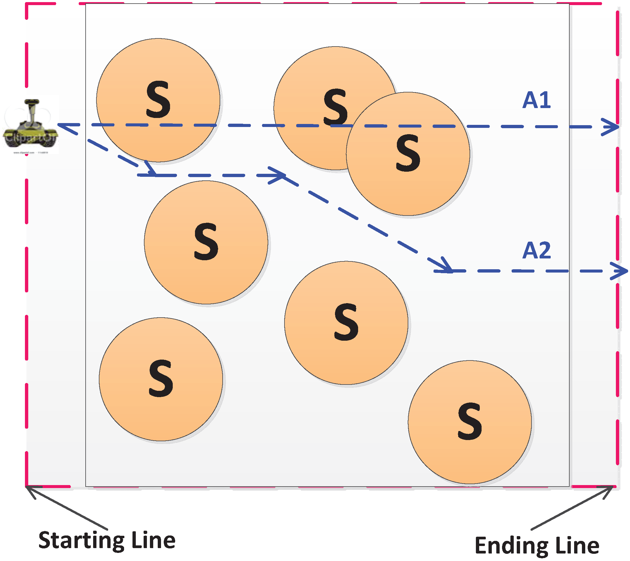
  • An intruder will enter the WSN FoI from any point along the left peripheral and move toward the right peripheral, aiming to traverse the WSN FoI and arrive at its destination outside of the FoI, as illustrated in Figure 1;
  • An intruder is able to detect nearby sensor(s) within its sensing range I r s ;
  • I r s > r s , which ensures that an intelligent intruder is able to sense nearby sensor(s) and perform detection avoidance before being detected by the WSN;
  • The terrain within the FoI will not affect sensor placement or the intruder’s intrusion path.
Figure 1. Illustration of an intelligent intruder detection problem formulation in a WSN. The intruder starts from a random point on the imaginary left periphery and moves toward another random point on the imaginary right periphery, which is the intruder’s destination. The intruder may adopt an AI-enabled intrusion algorithm (like A 2 ) for detection avoidance.
Futureinternet 08 00002 g001

2.2. Problem Formulation

The intelligent intruder detection problem in a WSN system can be formulated as a “game” according to “game theory” [24], which can be roughly abstracted as “a set of tools and a language for describing and predicting strategic behavior” [25], helping us abstract and understand how decision makers, i.e., the intelligent intruders, interact with the target WSN. In this paper, the interactions between an intruder and a WSN are terminated when either the intruder or the WSN wins. To be specific, the WSN is considered the “winner” if (1) the intruder is detected by a connected sensor before reaching its destination or (2) the intruder is still inside the WSN when the allotted time T m a x expires. Otherwise, the intruder is considered the “winner”. In other words, the intruder, modeled as an intelligent decision maker, is able to detect nearby sensors and take actions to circumvent the sensing coverage area of the WSN while heading for its destination.
Without loss of generosity and for the similarity of analysis and boundary effects’ avoidance, we formulate the given WSN field of interest A as a slightly bigger area with horizontal side length L + δ L ( δ L L ), while the vertical side length remains the same as L, as shown in Figure 1. The intruder will start from a random point on the imaginary left periphery and move toward another random point on the imaginary right periphery, which is the intruder’s destination.

2.3. Performance Evaluation Metrics

Based on the assumptions, models and problem formulation, we define the following performance metrics to study the impact of intruder’s intelligence on the intrusion detection capability of a WSN for various applications.
  • Detection probability P d e t : the probability that an intruder is detected by a connected sensor in a WSN within the maximum allowable intrusion time T m a x .
  • Prevention probability P p r e v t : the probability that an intruder is not detected, however is prevented from reaching its destination within the maximum allowable intrusion time T m a x .
  • WSN win probability P w s n : the sum of the detection probability P d e t and the prevention probability P p r e v t , and P w s n = P d e t + P p r e v t .
  • Escape probability P i n t r u : the probability that an intruder manages to escape the WSN FoI and arrives at the destination within the allotted T m a x .
In addition, we include the definitions for general WSN evaluation metrics including coverage, connectivity and connected coverage for the purpose of comparison [5]:
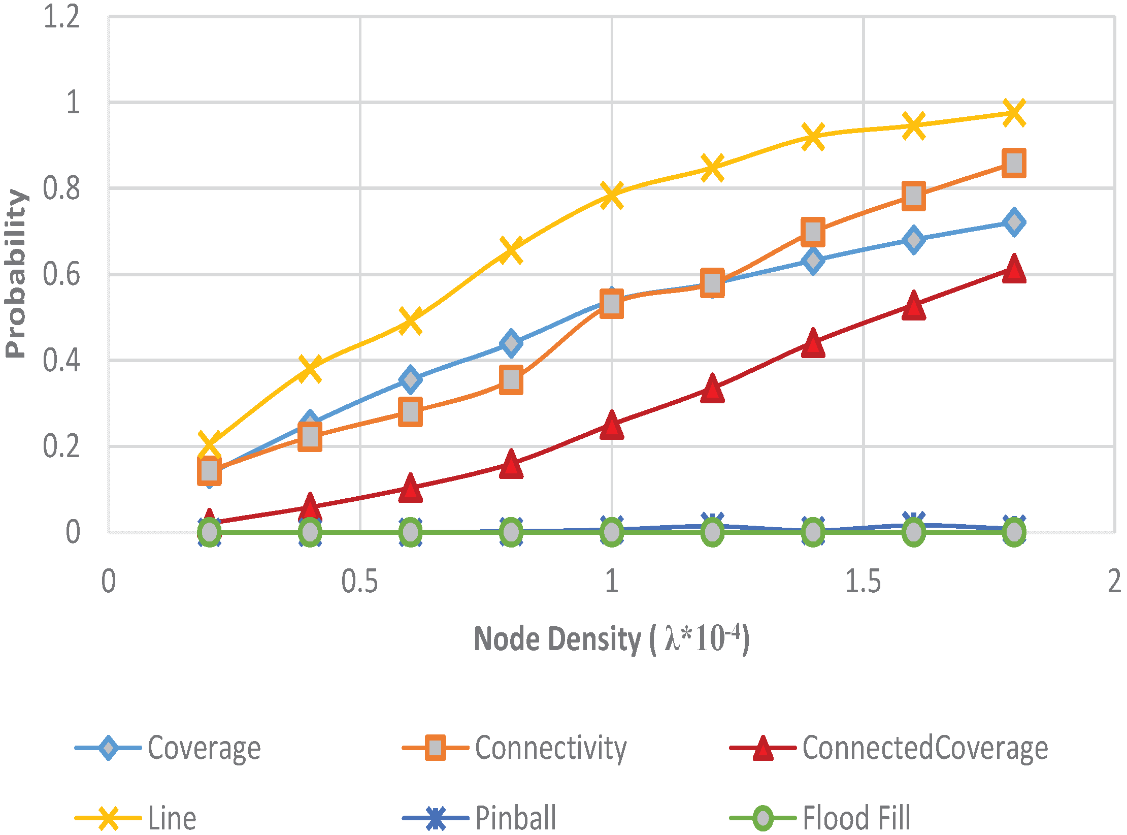
  • Coverage: Any point in the field of interest is said to be covered if it is within the sensing range of a sensor. The network coverage is defined as the probability of a random point in A being covered by at least one sensor.
  • Connectivity: Consider two random sensors s i and s j located inside A; s i and s j are connected if there exists a communication path between them. The network connectivity is defined as the probability of a random sensor that can communicate with the base station through a direct or multi-hop communication path, i.e., a connected sensor.
  • Connected coverage: An intruder is considered to be detected when it enters the sensing coverage area of a connected sensor (to the BS). The network connected coverage is thus defined as the probability of a random point in A that is covered by at least one connected sensor.
The notations used in this work are summarized in Table 1.

3. Intrusion Algorithms

In this section, three intrusion algorithms, including the linear intrusion, pinball intrusion and flood-fill intrusion algorithms, are presented.
Table 1. Notation table.
NotationDescription
LSide length of the field of interest
NNumber of sensors deployed
r s Sensing range
r c Communication range
I r s Intruder sensing range
λNode density
P d e t Detection probability
P p r e v t Prevention probability
P w s n WSN win probability
P i n t r u Intruder escape probability

3.1. Linear Intrusion Algorithm

Following the linear intrusion algorithm, the intruder will start from a source point on the imaginary starting line on the left side of the WSN FoI and follow a straight-line path toward the ending line on the right side. In Figure 1, A 1 illustrates an example linear intrusion path of a linear intruder.

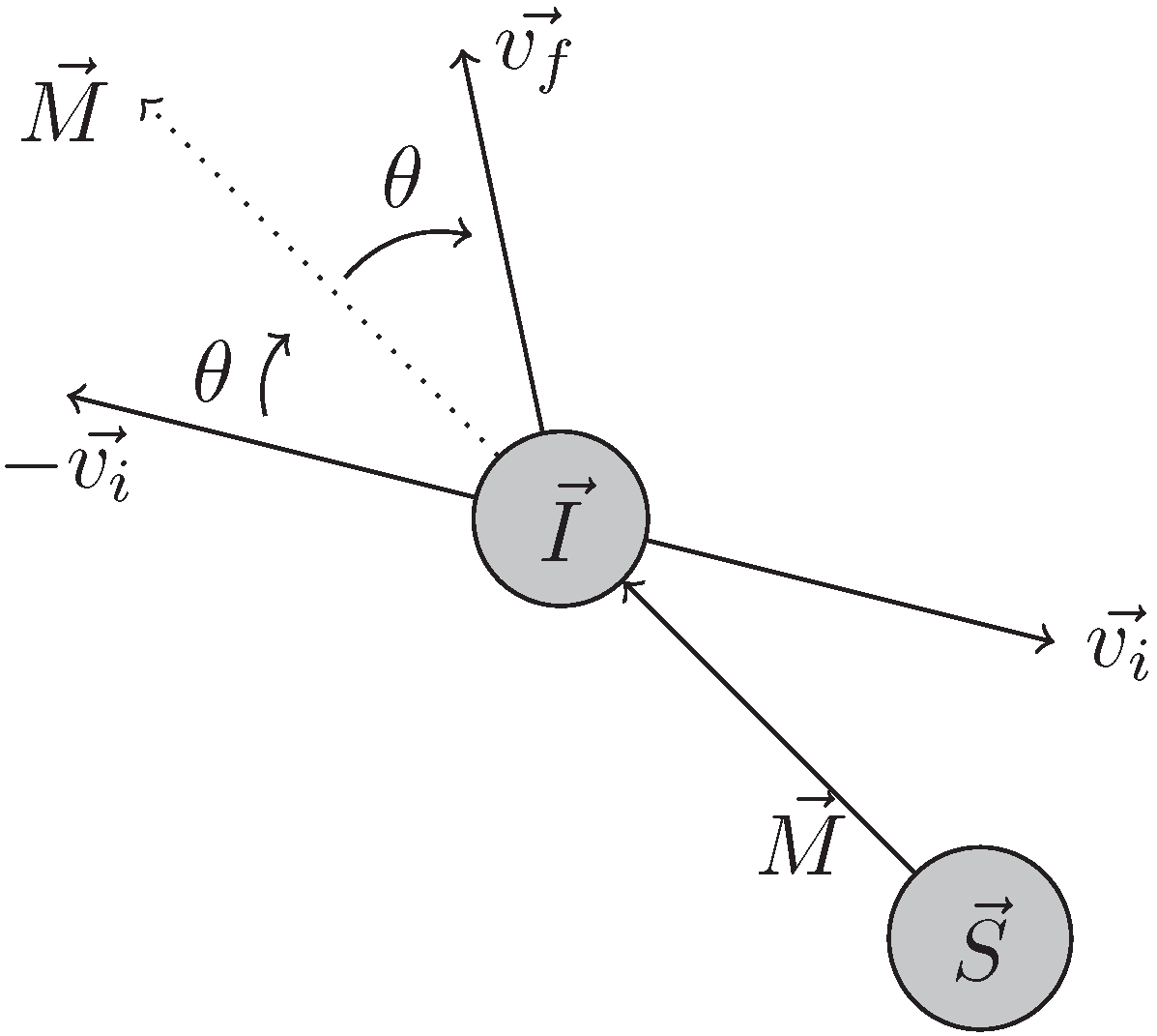
3.2. Pinball Intrusion Algorithm

Motivated by the kinetic theory behind billiards or pinball balls rebounding off a collision with equal kinetic energy [26,27], we propose the pinball algorithm for detection avoidance. Intruders following this detection avoidance strategy, called pinball intruders, will bounce away with a constant speed after encountering the boundaries of WSN FoI or detecting the sensing coverage area of a sensor within its sensing range I r s .
To be specific, the intruder starts its intrusion from the left periphery of the WSN FoI and moves toward the right periphery, aiming to safely pass the WSN and reach its destination in a timely manner. During its traversal, the intruder might sense a nearby sensor (within distance I r s ) or an edge of the FoI. If the intruder senses the left, upper, or bottom edge of the FoI, it will invert the x or y component of its velocity as if a ball hits the vertical or horizontal edges, respectively. On the other hand, if the intruder senses the sensing coverage area of a sensor that is modeled as a circular disk with radius r s , the normal of the reflection surface becomes the line between the intruder and the sensor. As illustrated in Figure 2, let I and S be the position vectors of the intruder and sensor detected. The x and y components of any vector A are denoted as A x and A y , respectively. The normal of the reflection surface is thus the mirror vector M = I S . Assume the intruder’s initial velocity is v i , and the resulting velocity is v f after bouncing off the sensor for collision avoidance. Using some vector math, v f can be computed by calculating the angle θ and performing a rotation on v i , as shown below.
θ = atan2 ( M y , M x ) atan2 ( v i y , v i y )
atan2 ( y , x ) = arctan y x ; ( x > 0 ) arctan y x + π ; ( y 0 , x < 0 ) arctan y x π ; ( y < 0 , x < 0 ) π 2 ; ( y > 0 , x = 0 ) π 2 ; ( y < 0 , x = 0 ) undefined , ( y = 0 , x = 0 )
Figure 2. Pinball algorithm.
Futureinternet 08 00002 g002
After solving for θ, twice that value is the angle that v i is to be rotated. Rotating v i by 2 θ gives the resultant velocity v f .
v f x = ( v i x ) c o s ( 2 θ ) ( v i y ) s i n ( 2 θ ) ; = v i x c o s ( 2 θ ) + v i y s i n ( 2 θ )
v f y = ( v i x ) s i n ( 2 θ ) + ( v i y ) c o s ( 2 θ ) ; = v i x s i n ( 2 θ ) v i x c o s ( 2 θ )
v f = v f x x ^ + v f y y ^
By setting the velocity to v f upon the intruder’s detection of any sensor or wall, the intruder avoids sensors by reflecting off of potential detection points. The pseudocode of the pinball intrusion algorithm is also described in Algorithm 1.
Note that some functionality is simplified into several functions to improve readability in Algorithm 1. To be specific:
  • n o r m a l i z e ( v ) performs vector normalization. It returns a vector that points in the same direction as the input vector, but with a length of one.
  • c o l l i d e s ( p , o b j ) performs sensor/wall detection between the entity’s original position and the next position p against the detected o b j (i.e., a sensor or an FoI boundary). In the case of an FoI boundary, the function will check for the intersection of two line segments. Additionally, in the case of a sensor, the function will check if p lies within the sensor’s circular disk of radius r s .
  • a n g l e B e t w e e n ( v 1 , v 2 ) finds the angle between the vectors v 1 and v 2 . The resulting value will utilize the a t a n 2 function defined in Equation (2).
    θ = a t a n 2 ( v 2 y , v 2 x ) a t a n 2 ( v 1 y , v 1 x )
  • v e c t o r R o t a t e ( v , θ ) returns the result of v rotated by θ around its origin.
Algorithm 1 Pinball.
1: while position ! = destination do
2:       velocity normalize ( destination position )
3:       nextPosition position + velocity
4:      if collides(nextPosition, horizontalWall) then
5:            velocity.y velocity.y
6:      if collides(nextPosition, verticalWall) then
7:            velocity.x velocity.x
8:      for all sensor in sensors do
9:           if collides(nextPosition, sensor) then
10:                 mirror position sensorPosition
11:                 angle angleBetween ( mirror , velocity )
12:                 negativeV velocity
13:                 velocity vectorRotate ( negativeV , 2 * angle )

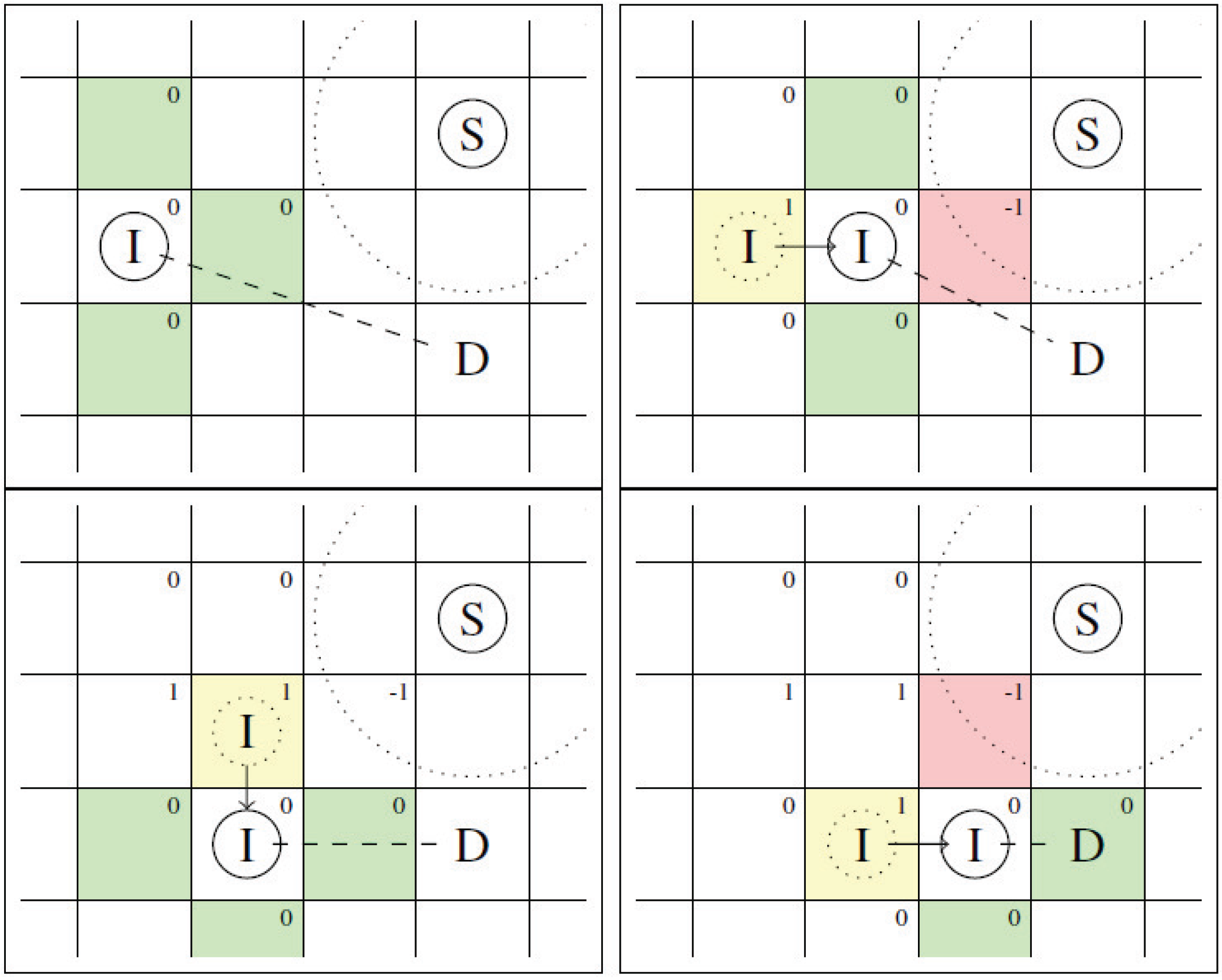
3.3. Flood-Fill Intrusion Algorithm

The pinball algorithm simply avoids collisions by bouncing off nearby sensors detected within its sensing range I r s . It does not estimate the cost to the destination for each state or efficiently store-and-update environment information with backtracking costs. In other words, while a pinball intruder can efficiently avoid sensor detection, it may become stuck or time-out inside the WSN FoI, i.e., it may not be able to reach the destination in a timely manner. In most WSN applications, an intruder’s primary goal is to safely traverse the WSN FoI and to arrive at its destination within a certain time. Hence, we propose a flood-fill intrusion algorithm that integrates environment learning, map building, updating, backtracking and path replanning for detection avoidance and timely destination arrival.
Different from the traditional flood-fill algorithms for maze-solving problems that require full prior knowledge of the environment, our proposed flood-fill algorithm assumes no prior knowledge of the WSN FoI. Instead, the flood-fill algorithm involves dividing the WSN FoI into a virtual m m grid map, and all cells in the map are initially “empty”, which represents no prior knowledge of the WSN FoI, as illustrated in Figure 3. The algorithm attempts to update the status of the cells by measuring and updating the WSN FoI status in terms of “safe” or “unsafe” and utilizes the learning information to direct the next move, until reaching the destination or experiencing a time-out.
Figure 3. An illustration of the flood fill algorithm.
Futureinternet 08 00002 g003
To start the algorithm, the intruder will choose a start position on the left extended periphery and a target position on the right extended periphery and will restrict all movements to the virtual grid, i.e., move from the center of one cell to the next one. On each move, as illustrated in Figure 3, the intruder must check its adjacent cells and update the cell values in the map to represent their sensing coverage status and the status of “visits”. To be specific:
  • If a cell c i is fully or partially covered by a detected sensor within r s , then the cell receives a value of 1 . Assume c ( x i , y i ) and s ( x j , y j ) are the locations of the cell c i , and the detected sensor s j . Cell c i will be considered as “unsafe” and receive a value of 1 if ( x i x j ) 2 + ( y i y j ) 2 < r s + 2 / 2 . Otherwise, cell c i is considered “safe” and receives a value of zero.
  • For a safe cell with a value of zero, the value will be incremented by one each time the intruder visits it. For instance, a cell with a value of three means the cell is visited by the intruder three times. This is because the intruder might have to backtrack under certain conditions.
During traversal, while the intruder has not reached its target position or experienced a time-out and when it comes to make a move, it will check all cells adjacent to it to see which one is should head to next. More specifically:
  • If a cell adjacent to the intruder has not been visited by the intruder before, it will check to see its coverage status first. Once the intruder has checked all adjacent cells, the intruder will proceed in the direction of the cell with the lowest value.
  • If multiple cells have the same value, the intruder will decide which direction to move based on the distance from each cell to its target position. For example, if the intruder needs to travel six units along the x-axis and three units along y-axis to reach its target position, it will first attempt to travel along the x-axis.
  • If that cell is not amongst those with the lowest value, then the intruder will go clockwise, checking the other cells for the lowest value, and will travel along the direction of the first lowest value cell it finds. Before the intruder leaves a cell, it will increment the value of that cell by one.
The pseudocode of the flood-fill intrusion algorithm is shown in Algorithm 2. Some critical functions and data structures are described as follows:
  • d i r e c t i o n s is an array containing the four basic directions: up ( < 0 , 1 > ), down ( < 0 , 1 > ), left ( < 1 , 0 > ) and right ( < 1 , 0 > ).
  • s t e p s is an array generated every loop containing the position of the intruder if it were to take each of the directions in d i r e c t i o n s
  • C o u n t ( a r r a y ) counts the number of elements in an array
  • m a p is a data structure mapping keys (cell positions) to values (cell values). Accessing a cell’s value is expressed as m a p [ p o s i t i o n ] .
Algorithm 2 Flood-fill.
1: while position ! = intruderDestinationPosition do
2:       for i = 0 ; i < Count(directions) ; i + + do
3:             steps[i] position + directions[i] * cellSize
4:       for i = 0 ; i < Count(directions) ; i + + do
5:            if ! map.containsKey ( directions[i] ) then
6:                 map[steps[i]] IsCovered(steps[i])
7:       for i = 0 ; i < Count(directions) ; i + + do
8:             hits[i] map[steps[i]]
9:        targetVector targetPosition - position
10:        maxDot
11:        generalDirection 1
12:       for i = 0 ; i < Count(directions) ; i + + do
13:             dot targetVector · directions[i]
14:            if dot > maxDot then
15:                 maxDot dot
16:                 generalDirection i
17:        min
18:        minHit 1
19:       for i = 0 ; i < Count(directions) ; i + + do
20:             j ( generalDirection + i ) % 4
21:            if hits[j] ! = 1 then
22:                if hits[j] < min then
23:                      min hits[j]
24:                      minHit j
25:       if minHit ! = 1 then
26:             position position + directions[minHit] * cellSize
27:             map[steps[minHit]] map[steps[minHit]] + 1

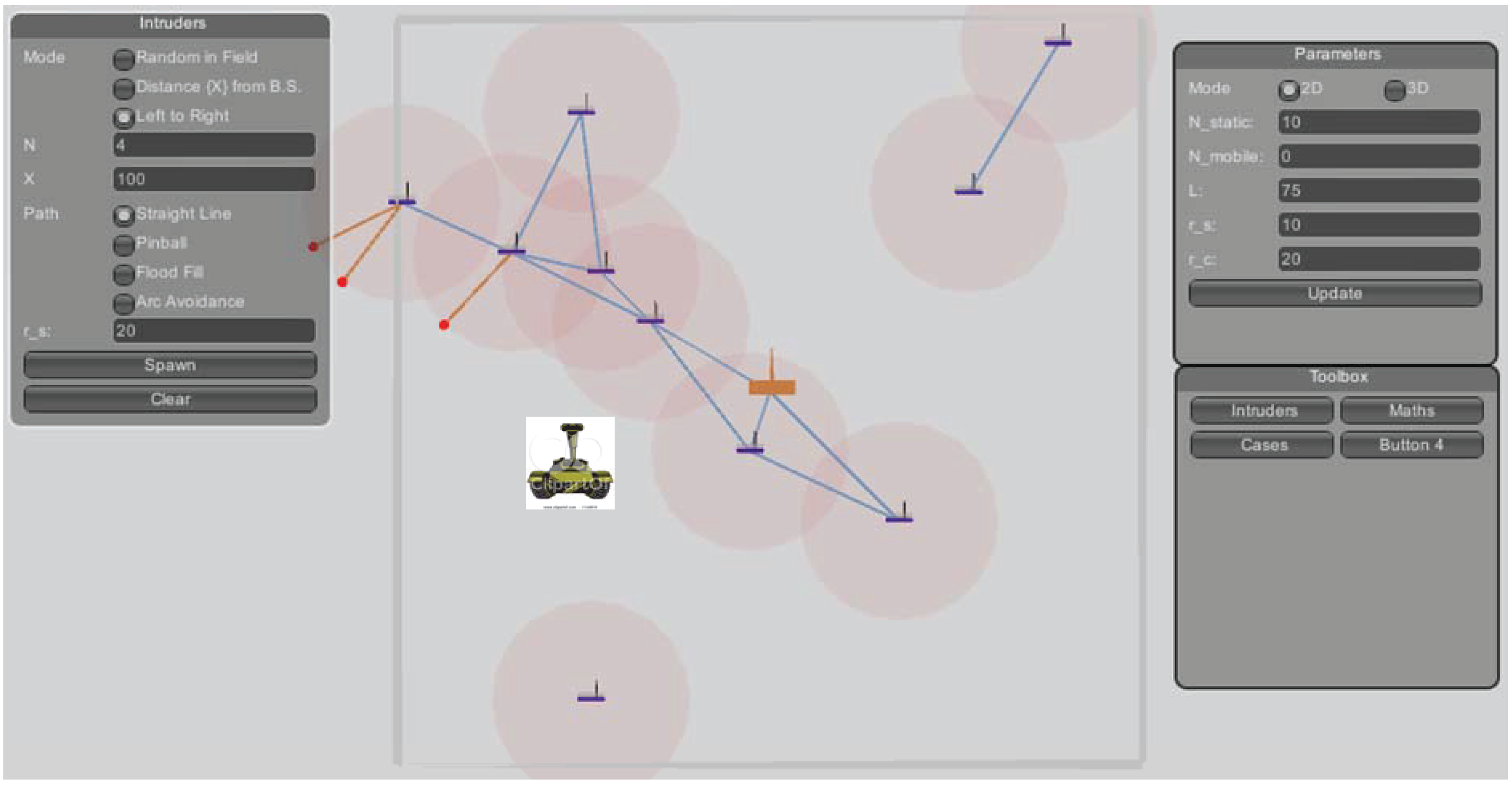
4. Demonstration, Simulation and Discussion

This section presents the simulation results and evaluates the impact of different intrusion algorithms on the intrusion detection problem of a WSN under various environments. We developed two simulators using the Unity platform [28,29] and C++ for demonstration and statistical analysis, respectively. Both simulators implement the three intrusion algorithms described in Section 3, capture the critical aspects of various WSNs and enable the interactions between intruders and WSNs. A screenshot of the simulator interface using Unity is demonstrated in Figure 4. The interface provides flexibility in selecting intrusion algorithms and configuring different WSN parameters for various settings. Moreover, Monte Carlo simulations are designed and conducted using the C++ simulator, aiming to examine the impact of different intrusion algorithms on the intrusion detection problem of a random WSN under various circumstances.
Figure 4. A screenshot of the simulator using the Unity platform.
Futureinternet 08 00002 g004

4.1. Impact of Node Density λ

First, we examine the impact of node density on the WSN win probability and the intruder’s escape probability, considering the three proposed intrusion algorithms. In this simulation, we fix L = 500 m, r s = 50 m and r c = 100 m and vary N from five to 45 to generate different node densities and network topologies. The intruder’s sensing range is set as I r s = 60 , unless otherwise specified. Figure 5, Figure 6 and Figure 7 illustrate the WSN win probability ( P w s n ), the escape probability ( P i n t r u ) and the network detection probability ( P d e t ) of an intruder that adopts the linear, pinball and flood-fill algorithms in random WSNs with varying node densities λ. All results plotted here are the average of 500 simulation runs under the same network settings. In each simulation run, we use two random variables, x and y, to generate the coordinates for each sensor in the FoI. In other words, 500 different network topologies within the considered node density range are generated and tested for statistical analysis in this section.
Figure 5. The WSN win probability ( P w s n ) of an intruder that adopts the linear, pinball and flood-fill algorithms in a WSN with varying node densities λ.
Futureinternet 08 00002 g005
Figure 6. The escape probability ( P i n t r u ) of an intruder that adopts the linear, pinball and flood-fill algorithms in a WSN with varying node densities λ.
Futureinternet 08 00002 g006
As Figure 5 and Figure 6 illustrate, the WSN win probability ( P w s n ) increases and the intruder’s escape probability ( P i n t r u ) decreases as the node density λ increases. This is because increased node density leads to higher connected coverage in the network field with a reduced safe area for the intruder to find a successful escape path. Second, there exist significant differences when an intruder traverses the same WSN field using different intrusion algorithms. Among the three considered algorithms, the flood-fill algorithm performs the best, while the pinball algorithm performs the worst. This is caused by the different design and implementation of detection avoidance strategies on the intruder side. To be specific, the pinball intruder simply avoids nearby sensors without taking into consideration the destination when adjusting its intrusion path. It then frequently moves to an area or position that is further away from the destination and results in the worst escape probability. This observation coincides with the results in a related work [16,30], “for an intruder, following a sine-curve intrusion path can be more beneficial than following a straight-line path as the probability of being detected can be substantially decreased, however, with a side effect of reducing intrusion progress towards the destination to some extent”. Namely, a linear intruder moves directly toward the destination without avoiding nearby sensors, and hence, it has a higher probability of escaping the WSN as compared to the pinball intruder. On the other hand, the flood-fill intruder aims to reach its destination and takes into consideration the destination when avoiding nearby sensors during its traversal and, thus, leads to the best performance in escaping the WSN field among the three algorithms.
Figure 7. The detection probability P d e t of an intruder that adopts the linear, pinball and flood-fill algorithms in a WSN with varying node densities λ.
Futureinternet 08 00002 g007
Figure 8 demonstrates the variances of the intruder’s escape probability ( P i n t r u ) of an intruder that adopts the linear, pinball and flood-fill algorithms versus node densities λ. As the node density increases, the escape probability ( P i n t r u ) of a pinball intruder gets closer to “0” most quickly while the flood-fill intruder gets the highest probability to escape the sensor field. This is caused by the different intelligent strategies applied in the intruder’s intrusion strategies. The results also suggest that there is a saturation point of the node density, after which deploying more sensors in the field of interest does not significantly decrease the intruder escape probability. The saturation point differs when the intruder takes different intrusion strategies.
Figure 8. The variances of the intruder’s escape probability ( P i n t r u ) of an intruder that adopts the linear, pinball and flood-fill algorithms in a WSN with varying node densities λ.
Futureinternet 08 00002 g008
It should be noted that the sensor detection avoidance strategy adopted by the pinball intruder may not be able to help improve its escape probability; however, it does help in reducing the detection probability ( P d e t ) to a significant extent. As illustrated in Figure 7, the detection probability of the considered WSN in detecting the intelligent pinball intruder and the flood-fill intruder approaches zero, while the detection probability of a linear intruder keeps increasing as the node density increases. The results confirm the necessity of integrating intruder’s intelligence in the WSN research for intruder detection for different applications.

4.2. Impact of Sensing Range r s

In this section, we examine the impact of sensing range r s on the WSN win probability ( P w s n ) and the intruder escape probability ( P i n t r u ). Again, we fix the network parameters as N = 25 , r c = 100 m, L = 500 m, A = 500 2 square meters and vary the the sensing range r s from 25 to 75 m. Figure 9 and Figure 10 illustrate the WSN win probability ( P w s n ) and the escape probability ( P i n t r u ) of an intruder that adopts the linear, pinball and flood-fill algorithms in random WSNs with varying sensing range r s . All results plotted here are the average of 500 simulation runs under the same network settings.
Figure 9. The WSN win probability ( P w s n ) of an intruder that adopts the linear, pinball and flood-fill algorithms in a WSN with varying sensing range r s .
Futureinternet 08 00002 g009
Figure 10. The escape probability ( P i n t r u ) of an intruder that adopts the linear, pinball and flood-fill algorithms in a WSN with varying sensing range r s .
Futureinternet 08 00002 g010
It is observed in Figure 9 and Figure 10 that, as the sensing range r s increases, the WSN win probability ( P w s n ) increases, and the intruder’s escape probability ( P i n t r u ) decreases for all three considered intruders. This is because the network sensing coverage increases as the increase of the sensing range r s , which makes it more difficult for the intruders to find a safe path to escape the WSN and reach their destination. Second, the WSN win probability ( P w s n ) in detecting and preventing the pinball intruder stays the highest, as indicated in Figure 9, and the pinball intruder performs the worst in escaping the WSN, as shown in Figure 10. This is because the pinball algorithm only avoids nearby sensors for detection avoidance without trying to make progress toward the destination. In addition, there exists a critical sensing range r s = 60 m, below which the WSN is shown to have the worst probability in preventing and detecting the flood-fill intruder. This is due to the best artificial intelligence strategies applied by the flood-fill intruder, including sensor detection, detection avoidance, map building, updating and backtracking, as described in Section 3.3. On the other hand, when the sensing range r s exceeds 60 m, the escape probability of the flood-fill intruder drops below the linear intruder and converges to the pinball intruder. This is caused by the high sensing coverage of the WSN when the sensing range exceeds 60 m, where the flood-fill intruder has to spend most of the time in avoiding nearby sensors instead of making progress toward the destination and, thus, gradually degrades to a pinball intruder.
The results in this section indicate that intelligent intruders may not always outperform the linear intruders when the network is well covered with a high sensing range. More specifically, there exists a critical sensing range, below which intelligent intruders have a higher probability of successfully traversing the WSN and reaching its destination and above which linear intruders outperform the intelligent intruders in terms of having a higher probability of reaching its destination.

4.3. Impact of Communication Range r c

To detect an intruder, a WSN should be well connected, so that detection can be reported to the base station. Namely, the network connectivity impacts the detection and prevention probability of a WSN and the escape probability of an intruder. The sensor’s communication range r c determines the network connectivity of a WSN. In order to examine the impact of communication range r c on the WSN win probability ( P w s n ) and the intruder’s escape probability ( P i n t r u ), we fix the network parameters as N = 25 , r s = 50 m, L = 500 m, A = 500 2 m 2 and vary the the communication range r c from 25 to 250 m. Each result plotted here is the average of 500 simulation runs under the same network settings.
Figure 11 and Figure 12 depict the WSN win probability ( P w s n ) and the escape probability ( P i n t r u ) of an intruder in traversing a WSN with varying communication ranges r c , taking into consideration the three considered intrusion algorithms. In the two figures, we have the following observations. First, the WSN win probability increases quickly in preventing and detecting the linear intruder, while that for the pinball and flood-fill intruders remains nearly constant as the communication range r c increases. This is because the network’s coverage remains the same with a constant number of deployed sensors N and sensing range r s . The same sensing coverage poses the same challenge for pinball and flood-fill intruders to detect and avoid sensors in their traversing. Namely, increased communication range has no contribution to the sensing coverage of the WSN. Thus, the WSN win probability of detecting and preventing pinball and flood-fill intruders keeps constant at the increase of the communication range r c . This also explains the nearly constant escape probability of the pinball and flood-fill intruder, as shown in Figure 12.
Figure 11. The WSN win probability ( P w s n ) of a WSN in detecting and preventing an intruder that adopts the linear, pinball and flood-fill algorithms in a WSN with varying communication range r c .
Futureinternet 08 00002 g011
On the other hand, it is observed that the WSN win probability of detecting and preventing the linear intruders increases, and the escape probability of the linear intruder drops with the increase of the communication range. This is because an increased communication range significantly contributes to the network connectivity and the connected coverage of a WSN. With increased communication range, more sensors that were initially isolated get connected to report the detection of the linear intruder to the base station. In other words, when the communication range is low, there exists a fraction of sensors that may be able detect the linear intruder within its sensing range; however, they may not able to report the detection to the base station for successful intruder detection. Hence, as the communication range increases, the probability that a linear intruder gets caught by a connected sensor increases, and its escape probability decreases accordingly.
Figure 12. The escape probability ( P i n t r u ) of an intruder that adopts the linear, pinball and flood-fill algorithms in a WSN with varying communication range r c .
Futureinternet 08 00002 g012
Moreover, we observe that there exist two critical communication ranges r c 1 = 60 and r c 2 = 120 . Specifically, when the communication range is below r c 1 , i.e., r c < r c 1 , the linear intruder outperforms the other two intelligent counterparts in terms of escape probability under the same network settings. Second, when the communication is above r c 2 , i.e., r c > r c 2 , both pinball and flood-fill intruders outperform the linear intruder, while the flood-fill intruder excels. Third, when the communication range is between the two critical ranges, i.e., r c 1 < r c < r c 2 , the flood-fill algorithm outperforms the linear algorithm, while the pinball algorithm performs the worst. The results indicate that intruder’s intelligence in detecting and avoiding nearby sensors has a significant impact on its escape probability, so as for the network connectivity.

4.4. Coverage, Connectivity, Connected Coverage versus Intruder Detection

From the above discussions, it is apparent that the general network quality of service (QoS), including sensing coverage, connectivity and connected coverage, has a significant impact on the detection probability of a WSN and the escape probability of an intruder. Therefore, it is important to examine the interplay between the general network QoS and the detection probability in a random WSN in Section 2.3.
Figure 13 illustrates the probability of coverage, connectivity, connected coverage and the detection probability of a random WSN in capturing linear, pinball and flood-fill intruders with varying node densities. In this simulation, we use the simulator to generate random topologies with different numbers of sensors ranging from five to 45 in an area of 500 × 500 square meters. Sensors are identical with a sensing range of r s = 50 m and a transmission range of r c = 100 m. In each case, we test 500 samples, and the probabilities are computed according to the definitions in Section 2.3.
Figure 13. Probability of coverage, connectivity, connected coverage and the detection probabilities of a random WSN with varying node densities λ.
Futureinternet 08 00002 g013
The simulation results in Figure 13 indicate that the coverage, the connectivity and the connected coverage all increase as the node density increases, and the probability of the connected coverage is always the lowest under the same network settings, as expected. Another observation is that the behaviors of both coverage and connectivity have similar tendencies over the node density and almost overlapped each other. This is because the communication range r c is set as twice the sensing range r s , i.e., r c = 2 r s in the study, which is a critical condition that a complete coverage of a convex WSN implies connectivity among the set of working sensors [31]. Last, but most importantly, the results demonstrate the significant differences among the coverage, connectivity, connected coverage and the detection probability of a WSN. More specifically, the probability of detecting a linear intruder is always higher than the network coverage, connectivity and connected coverage, while that of detecting the intelligent pinball and flood-fill intruders is always lower than the network coverage, connectivity and connected coverage. The results support our claim that: (1) existing results on general QoS in a WSN, including coverage, connectivity and connected coverage, cannot be directly applied to the intruder detection applications; and (2) intruder’s intelligence plays an important role in the detection probability of a WSN and requires a separate treatment in WSN research.

5. Conclusions

This work investigates the impact of intruder’s intelligence on the intrusion detection problem of a WSN under various circumstances for the first time. Two AI-enabled algorithms, pinball and flood-fill, are proposed and integrated into a WSN simulator for intrusion detection analysis. Simulation results demonstrate a significant impact of intruder’s intelligence on the intrusion detection probability of a WSN under various circumstances. In addition, network parameters, including node density, sensing range and communication range, have a crucial impact on the effectiveness of the intruder’s intrusion algorithms. It is therefore imperative to consider intruder’s intelligence in the design and deployment of WSNs for intrusion detection tasks. In the future, we are to consider more advanced path-planning strategies and study their impact on the intrusion detection problem in WSNs for various applications, aiming to provide practical insights into the real-life WSN design and implementation. The primary contribution of our work lies in the fact that it expands the knowledge of WSN research, leads to new research directions, and provides foundations for research in the field of WSNs for real-life intruder detection. We plan to investigate additional network factors, such as access delays, collisions, repetitions, routing, etc., on the detection capability of a WSN, taking into consideration advanced environmental learning and path planning algorithms.

Author Contributions

Y. W. conceived and directed the project; The remaining authors are students who all substantially contributed to the implementation of the project and the writing sections of this paper.

Conflicts of Interest

The authors declare no conflict of interest.

References

  1. Yang, H.; Sikdar, B. A protocol for tracking mobile targets using sensor networks. In Proceedings of the First IEEE International Workshop on Sensor Network Protocols and Applications, Anchorage, AK, USA, 11 May 2003; pp. 71–81.
  2. Yick, J.; Mukherjee, B.; Ghosal, D. Wireless sensor network survey. Comput. Netw. 2008, 52, 2292–2330. [Google Scholar] [CrossRef]
  3. Bokareva, T.; Hu, W.; Kanhere, S.; Ristic, B.; Gordon, N.; Bessell, T.; Rutten, M.; Jha, S. Wireless sensor networks for battlefield surveillance. In Proceedings of the Land Warfare Conference, Brisbane, Australia, 24-27 October 2006; pp. 1–8.
  4. Hamdi, M.; Boudriga, N.; Obaidat, M.S. WHOMoVeS: An optimized broadband sensor network for military vehicle tracking. Int. J. Commun. Syst. 2008, 21, 277–300. [Google Scholar] [CrossRef]
  5. Severino, R.; Alves, M. Engineering a search and rescue application with a wireless sensor network-based localization mechanism. In Proceedings of the IEEE International Symposium on a World of Wireless, Mobile and Multimedia Networks, WoWMoM 2007, Espoo, Finland, 18–21 June 2007; pp. 1–4.
  6. Sharp, C.; Schaffert, S.; Woo, A.; Sastry, N.; Karlof, C.; Sastry, S.; Culler, D. Design and implementation of a sensor network system for vehicle tracking and autonomous interception. In Proceedings of the Second European Workshop on Wireless Sensor Networks, Istanbul, Turkey, 31 January–2 February 2005; pp. 93–107.
  7. Tsai, H.W.; Chu, C.P.; Chen, T.S. Mobile object tracking in wireless sensor networks. Comput. Commun. 2007, 30, 1811–1825. [Google Scholar] [CrossRef]
  8. Bhatti, S.; Xu, J. Survey of target tracking protocols using wireless sensor network. In Proceedings of the Fifth International Conference on Wireless and Mobile Communications, ICWMC’09, Cannes, France, 23–29 August 2009; pp. 110–115.
  9. Dyo, V.; Ellwood, S.A.; Macdonald, D.W.; Markham, A.; Mascolo, C.; Pásztor, B.; Scellato, S.; Trigoni, N.; Wohlers, R.; Yousef, K. Evolution and sustainability of a wildlife monitoring sensor network. In Proceedings of the 8th ACM Conference on Embedded Networked Sensor Systems, Zurich, Switzerland, 3–5 November 2010; pp. 127–140.
  10. Lazos, L.; Poovendran, R.; Ritcey, J.A. Analytic evaluation of target detection in heterogeneous wireless sensor networks. ACM Trans. Sens. Netw. 2009, 5, 1–18. [Google Scholar] [CrossRef]
  11. Gui, C.; Mohapatra, P. Power conservation and quality of surveillance in target tracking sensor networks. In Proceedings of the 10th Annual International Conference on Mobile Computing and Networking, Philadelphia, PA, USA, 26 September–1 October 2004; pp. 129–143.
  12. Arora, A.; Dutta, P.; Bapat, S.; Kulathumani, V.; Zhang, H.; Naik, V.; Mittal, V.; Cao, H.; Demirbas, M.; Gouda, M.; et al. A line in the sand: A wireless sensor network for target detection, classification, and tracking. Comput. Netw. 2004, 46, 605–634. [Google Scholar] [CrossRef]
  13. Lazos, L.; Poovendran, R.; Ritcey, J.A. Probabilistic detection of mobile targets in heterogeneous sensor networks. In Proceedings of the 6th International Conference on Information Processing in Sensor Networks, Cambridge, MA, USA, 25–27 April 2007; pp. 519–528.
  14. Agah, A.; Das, S.K.; Basu, K.; Asadi, M. Intrusion detection in sensor networks: A non-cooperative game approach. In Proceedings of the Third IEEE International Symposium on Network Computing and Applications, (NCA 2004), Cambridge, MA, USA, 30 August–1 September 2004; pp. 343–346.
  15. Wang, Y.; Wang, X.; Xie, B.; Wang, D.; Agrawal, D.P. Intrusion detection in homogeneous and heterogeneous wireless sensor networks. IEEE Trans. Mob. Comput. 2008, 7, 698–711. [Google Scholar] [CrossRef]
  16. Wang, Y.; Leow, Y.K.; Yin, J. Is straight-line path always the best for intrusion detection in wireless sensor networks. In Proceedings of the 2009 15th International Conference on Parallel and Distributed Systems (ICPADS), Shenzhen, China, 8–11 December 2009; pp. 564–571.
  17. Hart, P.E.; Nilsson, N.J.; Raphael, B. A formal basis for the heuristic determination of minimum cost paths. IEEE Trans. Syst. Sci. Cybern. 1968, 4, 100–107. [Google Scholar] [CrossRef]
  18. Rao, N.S.V. An algorithmic framework for navigation in unknown terrains. IEEE Comput. 1989, 22, 37–43. [Google Scholar] [CrossRef]
  19. Cao, Q.; Yan, T.; Stankovic, J.; Abdelzaher, T. Analysis of target detection performance for wireless sensor networks. In Distributed Computing in Sensor Systems; Springer: Berlin, Heidelberg, 2005; pp. 276–292. [Google Scholar]
  20. Wang, Y.; Fu, W.; Agrawal, D.P. Gaussian versus uniform distribution for intrusion detection in wireless sensor networks. IEEE Trans. Parallel Distrib. Syst. 2013, 24, 342–355. [Google Scholar] [CrossRef]
  21. Camp, T.; Boleng, J.; Davies, V. A survey of mobility models for ad hoc network research. Wirel. Commun. Mob. Comput. 2002, 2, 483–502. [Google Scholar] [CrossRef]
  22. Liu, B.; Brass, P.; Dousse, O.; Nain, P.; Towsley, D. Mobility improves coverage of sensor networks. In Proceedings of the 6th ACM International Symposium on Mobile Ad Hoc Networking and Computing, Chicago, IL, USA, 25–28 May 2005; pp. 300–308.
  23. Keung, Y.; Li, B.; Zhang, Q. The intrusion detection in mobile sensor network. In Proceedings of the Eleventh ACM International Symposium on Mobile Ad Hoc Networking and Computing, Chicago, IL, USA, 20–24 September 2010; pp. 11–20.
  24. Morris, P. Introduction to Game Theory; Springer Science & Business Media: New York, NY, USA, 1994. [Google Scholar]
  25. Picker, R.C. An Introduction to Game Theory and the Law; Law School, University of Chicago: Chicago, IL, USA, 1994. [Google Scholar]
  26. Cutnell, J.D.; Johnson, K.W. Physics; John Wiley & Sons: Hoboken, NJ, USA, 2009. [Google Scholar]
  27. Kinetic Theory. Available online: http://physics.bu.edu/ duffy/py105/Kinetictheory.html (accessed on 18 April 2015).
  28. Unity3D. Available online: http://unity3d.com/unity (accessed on 28 March 2015).
  29. Blackman, S. Beginning 3D Game Development with Unity: All-in-One, Multi-Platform Game Development; Apress: New York, NY, USA, 2011. [Google Scholar]
  30. Wang, Y.; Leow, Y.K.; Yin, J. A novel sine-curve mobility model for intrusion detection in wireless sensor networks. Wirel. Commun. Mob. Comput. 2013, 13, 1555–1570. [Google Scholar] [CrossRef]
  31. Zhang, H.; Hou, J.C. Maintaining sensing coverage and connectivity in large sensor networks. Ad Hoc Sens. Wirel. Netw. 2005, 1, 89–124. [Google Scholar]

