Speech Inpainting Based on Multi-Layer Long Short-Term Memory Networks

Abstract

Audio inpainting plays an important role in addressing incomplete, damaged, or missing audio signals, contributing to improved quality of service and overall user experience in multimedia communications over the Internet and mobile networks. This paper presents an innovative solution for speech inpainting using Long Short-Term Memory (LSTM) networks, i.e., a restoring task where the missing parts of speech signals are recovered from the previous information in the time domain. The lost or corrupted speech signals are also referred to as gaps. We regard the speech inpainting task as a time-series prediction problem in this research work. To address this problem, we designed multi-layer LSTM networks and trained them on different speech datasets. Our study aims to investigate the inpainting performance of the proposed models on different datasets and with varying LSTM layers and explore the effect of multi-layer LSTM networks on the prediction of speech samples in terms of perceived audio quality. The inpainted speech quality is evaluated through the Mean Opinion Score (MOS) and a frequency analysis of the spectrogram. Our proposed multi-layer LSTM models are able to restore up to 1 s of gaps with high perceptual audio quality using the features captured from the time domain only. Specifically, for gap lengths under 500 ms, the MOS can reach up to 3~4, and for gap lengths ranging between 500 ms and 1 s, the MOS can reach up to 2~3. In the time domain, the proposed models can proficiently restore the envelope and trend of lost speech signals. In the frequency domain, the proposed models can restore spectrogram blocks with higher similarity to the original signals at frequencies less than 2.0 kHz and comparatively lower similarity at frequencies in the range of 2.0 kHz~8.0 kHz.

1. Introduction

In various audio processing tasks, audio signals often experience unexpected damage and information loss, which causes “gaps” within the audio signal. The process of restoring the gaps in the audio signal is called audio inpainting [1], which is also known as audio interpolation [2,3,4,5,6], extrapolation [7,8], waveform substitution [9], and imputation [10,11]. The term “inpainting” is adopted from image inpainting in the computer vision and image processing fields, which is a technique related to restoring the missing or corrupted parts of an image [12]. Audio inpainting is a general concept that includes restoring any audio signal, such as speech, music, instrument, environmental sounds, or any other auditory signals. It can be referred to as speech inpainting when applied to speech signals. As such, it is a specific form of audio inpainting.

In real-life applications, clean speech signals are often affected by many factors, such as degradation of audio quality, loss of information, and unpredictable noise [13], which leads to the incomplete transmission of speech signals, making it difficult for users at both the sending and receiving ends to communicate with each other. Speech inpainting aims to restore coherent and meaningful samples to the missing parts of a speech signal, ensuring that users at the receiving end do not perceive any information loss. In this paper, we propose an innovative speech inpainting mechanism to restore speech signal losses of up to one second using multi-layer Long Short-Term Memory (LSTM) networks [14].

Currently, there are two kinds of methodology used in the context of the audio inpainting task: mathematical-based approaches and deep learning-based algorithms. Previous research on audio inpainting mainly focused on using mathematical signal-processing techniques [1,2,3,4,5,6,7,8,10,11,15,16,17,18,19,20,21]. In recent years, with the gradual maturity of deep learning technology, researchers have begun to use deep learning-based audio inpainting algorithms to restore lost information in audio signals [22,23,24,25,26,27,28,29,30,31].

However, it should be noted that existing speech inpainting techniques primarily rely on “specific conditions” to restore the missing information. For example, SpeechPainter [27] is designed exclusively for text-based data, which means that during the inpainting process, all the speech transcripts are used to achieve outstanding predictions. Other techniques utilise visual information-based approaches, like facial motions together with the context information, to address the restoration task, as proposed in [31]. It is worth mentioning that during the signal transmission process in communication systems, such “specific conditions” do not exist except for the information before and after the missing area, which means that the loss of information is permanent and irreversible. Therefore, the methods mentioned above cannot be universally applied to all types of inpainting tasks due to their inherent limitations, which means that a new approach is needed.

In this paper, we propose a method for addressing speech inpainting using multi-layer LSTM networks. A series of LSTM networks containing between two and six layers were designed and trained on four single-speaker datasets, followed by further training on four multi-speaker datasets using an exclusive five-layer LSTM network. Our research is based on two types of datasets—single-speaker and multi-speaker datasets—to investigate the inpainting performance of the proposed LSTM models in terms of the perceived audio quality with different LSTM layers, datasets, and gap lengths. The performance is evaluated through the Mean Opinion Score (MOS) [32] and frequency analysis method [33] to assess the inpainted speech quality. Our proposed models are capable of learning information prior to the gap and inpainting coherently predicted speech samples to fill in missing gaps in the range of 20 ms–1000 ms.

The primary contribution of this paper lies in addressing speech inpainting in real-world communication scenarios, utilising only the voice information preceding the gap. In two-way real-time conversational communication, supplementary information, such as visual data, transcripts, and speech signals immediately following the gap, is not always available or feasible to use in speech inpainting. Using this supplementary information requires buffering a large amount of data and significant processing capability, resulting in lengthy jitter and degraded quality of service and user experience. The proposed speech-inpainting technique provides effective speech restoration without the need for supplementary information and achieves remarkable restoration effects and superior speech quality across gaps of varying lengths, significantly outperforming existing deep learning- and generative-based methods [22,23,24,25,26,27,28,29,30,31] that use supplementary information. This study not only contributes to the advancement of speech inpainting technology but also carries practical implications for applications such as speech enhancement and audio restoration.

The remainder of this paper is structured as follows. Section 2 presents the related works corresponding to our study. Section 3 illustrates the proposed methodology, model architecture, evaluation methods, and fine-tuning of the hyperparameters. Section 4 presents the experimental and training setup. Section 5 illustrates the results and analysis of the study. Section 6 presents the conclusions and suggests some future research directions.

2. Related Works

2.1. Conventional Audio Inpainting Based on Mathematics

Existing mathematical-based audio inpainting methods can be traced back to the last century. Early attempts at audio inpainting utilised spectral subtraction techniques for speech signal denoising, laying the foundation for subsequent audio restoration methods [34]. Atal proposed a linear prediction method to model the spectral envelope of speech signals, which can be used to restore missing gaps through linear prediction parameters; however, it cannot handle complex audio structures and non-stationary signals [35].

Considering the combination of statistical models, several studies have proposed the use of auto-regressive models to capture the correlation and structure within audio signals. Subsequently, the missing samples were inpainted and filled into corresponding positions through interpolation [2,3,4]. Furthermore, Lagrange et al. proposed an algorithm for sinusoidal component interpolation in the context of sinusoidal modelling, which can achieve a more realistic insertion of lost audio samples, especially in the case of musical modulations such as vibrato or tremolo [5,6]. To extend the duration of the restored audio samples, a longer audio extrapolation method was proposed in [7,8]. Considering the possibility of restoring lost audio signals in the time-frequency domain, Smaragdis et al. proposed a method to estimate missing spectrograms in the time-frequency domain of audio signals, which can process real-world polyphonic signals through imputation [10,11]. A more popular method is the sparsity-based approach [1,17,18,19,20,21], which aims to find the sparse representation of the missing part of the signal that best fits the surroundings [36].

In addition, there is another concept called Packet Loss Concealment (PLC) [15,16], which is similar to audio inpainting but specifically focuses on mitigating the impact of lost or corrupted packets in digital audio coding and communication systems. Both PLC and audio inpainting restore the loss of information, but they operate in different contexts and are based on different methodological foundations.

It is worth mentioning that the methods discussed above can only perform well in restoring millisecond-level gap lengths, roughly in the range of 10 ms–100 ms. For larger gaps, the restoration task tends to fail at producing plausible reconstructions, as the stationarity condition does not hold [36].

2.2. Deep Learning-Based Audio Inpainting Methods

In recent years, there has been an increase in the audio inpainting literature based on deep learning methods. Several key considerations need to be clarified in the context of the deep learning-based audio inpainting task, which can be summarised by three characteristics: the type of processed audio signal, the duration of the missing audio gap, and the deep learning method used.

Several studies have explored the efficacy of DNNs in addressing audio inpainting. Marafioti et al. utilised a DNN architecture to restore the missing part within an instrument’s audio signal using time-frequency coefficients (TF coefficients) [22], where the length of the inpainting gap was up to 128 ms. Similarly, Kegler et al. proposed an end-to-end DNN with a U-Net architecture to restore missing or distorted speech signals of up to 400 ms [23]. These works have shown that the DNN architecture can perform well in audio inpainting.

Generative Adversarial Networks (GANs) [24] have recently become a focal point in audio inpainting. Ebner et al. proposed to use the Wasserstein GAN (WGAN) to restore the lost part within an instrument’s audio signals based on short contexts (1 s from each side of the gap) and long contexts (2.5 s from each side of the gap), where the length of the inpainting gap was up to 550 ms [25]. Furthermore, [26] demonstrated that by using a conditional GAN (cGAN) model, missing audio segments could be restored based on the context of the surrounding audio and the latent variable of the cGAN. The authors aimed at restoring an instrument’s audio signals, where the lengths of the inpainting gap were up to 1500 ms.

It is worth noting that most of the approaches mainly focused on restoring music/instrument signals, which generally have long-term dependency and periodicity. In contrast, speech signals have more features and higher complexity when faced with several practical applications. Recent studies have noted the differences between music/instrument signal datasets and speech signal datasets [23,27,31]. Increasingly, researchers have started focusing on speech signals and using speech datasets to address audio inpainting.

As proposed in [27], the architecture of Perceiver IO [28] was used to restore the missing parts of speech signals according to the text transcript. The authors used a transformer-based model [29] to restore gaps of up to 1000 ms. Another study [30] proposed the use of a multi-modal transformer together with high-level visual features to restore an instrument’s audio signal, with gap lengths of up to 1600 ms. Other works, like [31], used visual information (facial motions) together with the audio context to restore gaps of up to 1600 ms within speech signals.

However, when comes to real-life two-way conversational communication scenarios, there are notable limitations shared by these approaches—they are all based on specific conditions. These conditions include the type of processed audio signal [22], relatively shorter gaps [23,25], the context before and after the gap [24], a text transcript [27,28], and visual information [30,31]. This limits the usage of the approaches in the literature to only their specific domains, as these conditions are not always available or feasible to use. This limitation underscores the necessity for further research in developing speech inpainting models that better align with practical communication scenarios.

3. Proposed Speech Inpainting Methods and Model Architecture

3.1. Long Short-Term Memory Networks

LSTM is a type of Recurrent Neural Network (RNN) architecture [37], which is designed to address the limitations of traditional RNNs in capturing long-distance dependencies and avoiding the vanishing gradient problem [14]. The vanishing gradient problem of the RNN model often occurs when the gradient of the loss function relative to the network weight becomes extremely small, which makes it difficult for RNNs to learn long-term correlations.

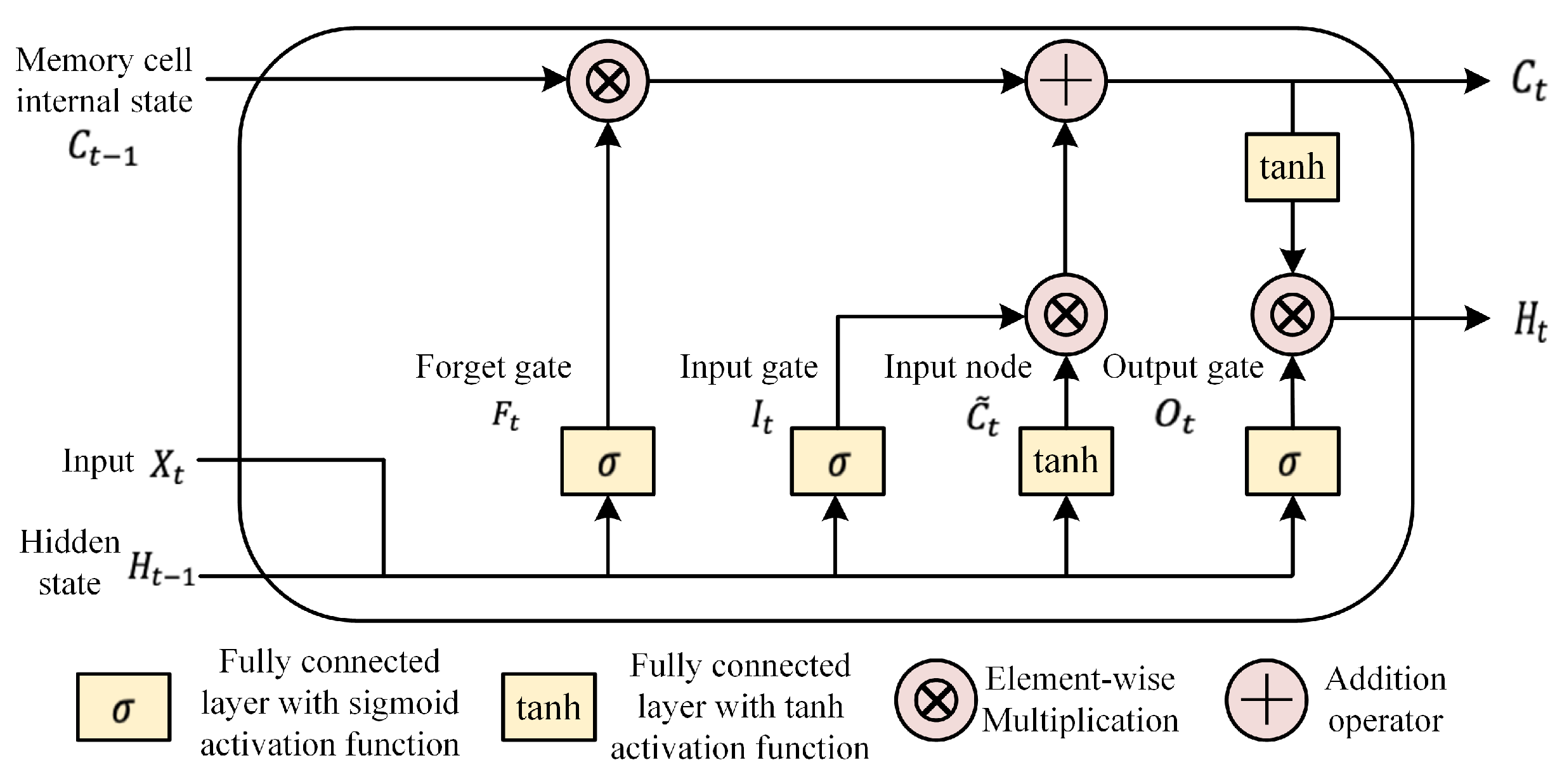
The structure of an LSTM cell is shown in Figure 1. By incorporating an input gate, forget gate, and output gate, the LSTM architecture has the ability to retain long-term memory of past inputs and their contextual information. Mathematically, let us denote the input time series as $X_t$, the hidden state of memory cells as $H_t$, the input gate as $I_t$, the forget gate as $F_t$, and the output gate as $O_t$, where $t\in [1,N]$ represents the time parameters. Then, we have the following notations:

$$\begin{array}{cc}\hfill I_t& =\sigma \left(X_t{W}_{xi}+H_{t-1}{W}_{hi}+b_i\right),\hfill \\ \hfill F_t& =\sigma \left(X_t{W}_{xf}+H_{t-1}{W}_{hf}+b_f\right),\hfill \\ \hfill O_t& =\sigma \left(X_t{W}_{xo}+H_{t-1}{W}_{ho}+b_o\right),\hfill \\ \hfill {\tilde{C}}_t& =tanh\left(X_t{W}_{xc}+H_{t-1}{W}_{hc}+b_c\right),\hfill \\ \hfill C_t& =F_t\otimes C_{t-1}+I_t\otimes {\tilde{C}}_t,\hfill \\ \hfill H_t& =O_t\otimes tanh\left(C_t\right),\hfill \end{array}$$

(1)

where W represents the weight parameters, b represents the bias parameters, and $\sigma$ represents the sigmoid activation function.

The input gate controls how much new information is added to the memory cell. The forget gate determines which information to discard from the memory cell. The output gate controls how much of the current memory cell state to feed to the next hidden state. In summary, the parameters inside the memory cell and the three gates are learned through backpropagation, allowing the network to selectively store and retrieve information over time and learn long-term dependencies in sequential data.

3.2. Series Prediction LSTM Model in Speech Inpainting

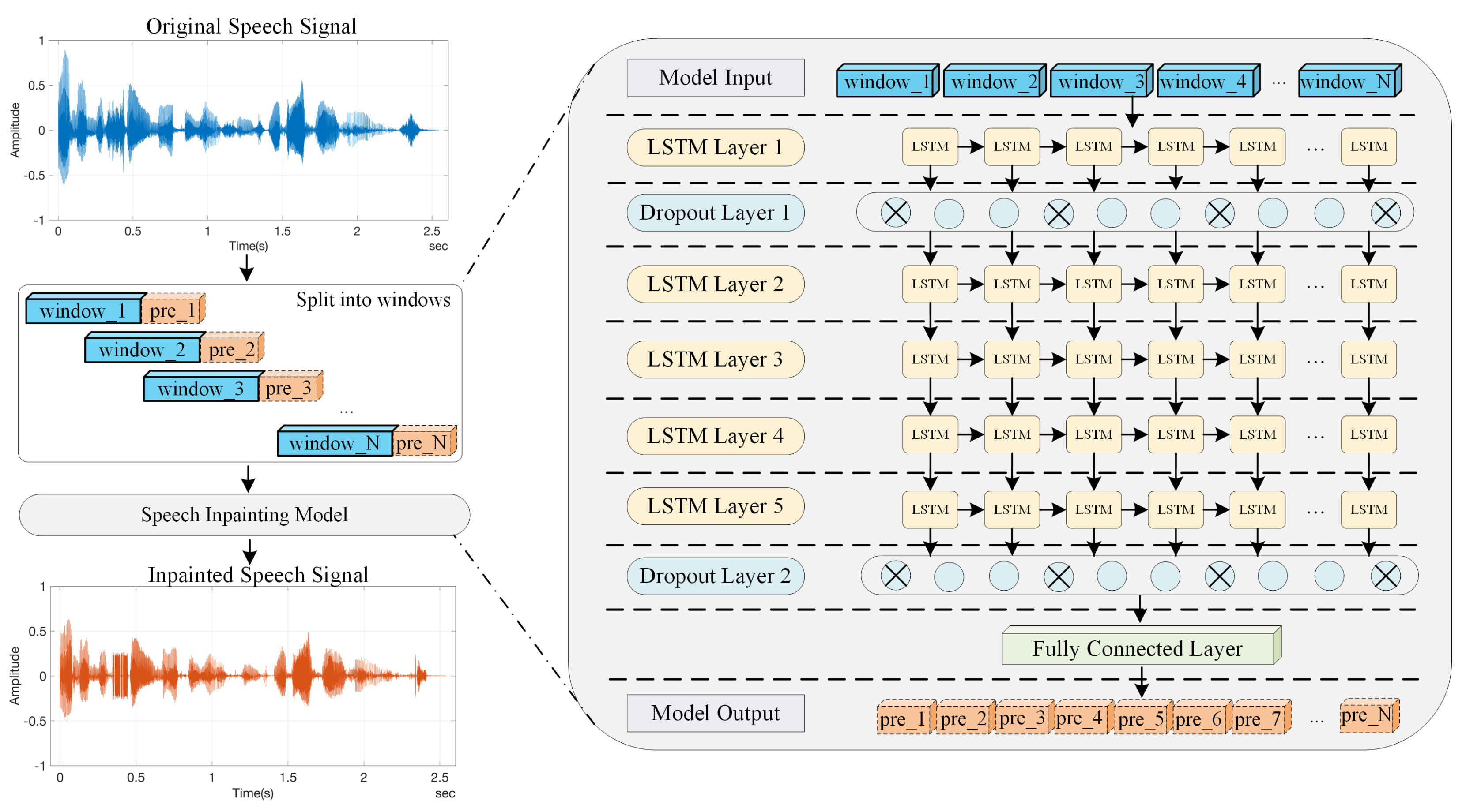
An LSTM model was constructed, as shown in Figure 2. The left side of the figure shows the proposed speech inpainting process applied in this work, and the right side shows the structure of the LSTM model. Note that only a five-layer LSTM model is depicted here.

The utilisation of LSTM in speech inpainting was motivated by its exceptional ability to capture complex temporal dependencies in spoken language. For processing and predicting time-series data such as speech signals, the capability of LSTM in modelling long-term temporal relationships, adapting to variable-length contexts, preserving contextual information, and learning hierarchical representations renders it well suited for this work.

During the speech inpainting process, the original speech signals are first split into multiple windows, labelled as $window\_i,\forall i\in [1,N]$, where N is the total number of windows split from the original speech signal, corresponding to the blue blocks in Figure 2. The length of each window is a fixed value of 640 speech samples, corresponding to a 40 ms speech signal when the signal is sampled at 16 kHz.

Subsequently, the split windows are fed into the LSTM model to obtain a series of prediction blocks, labelled as $pre\_\lambda$, where $\forall \lambda \in [1,N]$, and $\lambda$ is the number of predicted blocks in the inpainted speech signal, corresponding to the orange blocks in Figure 2. The length of each predicted block is 80 speech samples, corresponding to a 5 ms speech signal at a 16 kHz sampling rate. During each prediction process, the LSTM model predicts and outputs the results according to each input window in turn. After predicting a block, the window will shift 80 speech samples to form a new window of 640 speech samples and then repeat the prediction process. At the end of the inpainting process, all the predicted blocks (the orange-coloured ones in the figure) are concatenated to obtain the resulting inpainted speech signal, as shown at the bottom of the left-hand side of the figure.

3.3. Datasets

The datasets used in this research work were constructed from four widely used publicly accessible speech datasets: the LJ Speech dataset [38], the Hi-Fi multi-speaker dataset [39], the RyanSpeech dataset [40], and the LibriSpeech dataset [41]. Two categories of eight speech datasets were built for training and testing the proposed models. The first category contains four single-speaker datasets: one from the LJSpeech dataset, one from the RyanSpeech dataset, and two from the LibriSpeech dataset. The second category contains four multi-speaker datasets: one from the Hi-Fi multi-speaker dataset and three from the LibriSpeech dataset. The details of the datasets constructed in this research are shown in

Table 1. Datasets built in this research work.

Category	Dataset	Component (M: Male; F: Female)	Length (s)
Single-speaker	LJSpeech [38]	1 speaker (F)	400
	RyanSpeech [40]	1 speaker (M)	400
	LibriSpeech [41]	1 speaker (M)	400
	LibriSpeech [41]	1 speaker (F)	400
Multi-speaker	Hi-Fi [39]	10 speakers (4 F, 6 M)	400 for each speaker
	LibriSpeech [41]	10 speakers (5 F, 5 M)	400 for each speaker
	LibriSpeech [41]	10 speakers (5 F, 5 M)	400 for each speaker
	LibriSpeech [41]	10 speakers (5 F, 5 M)	400 for each speaker

:

• Single-speaker dataset:
  The first two datasets were built directly from the original LJSpeech and RyanSpeech datasets. The last two datasets were built from the LibriSpeech dataset, specifically from the “train-clean-100” folder, which contains speech data from multiple male and female speakers. The third dataset uses “folder 26” and the fourth uses “folder 32”. In this paper, these four datasets are referred to as LJSpeech, RyanSpeech, Libri_26, and Libri_32. Each dataset collates 400-second-long female or male speech samples at a 16 kHz sampling rate and contains one speaker.
• Multi-speaker dataset:
  The first dataset was built from the original Hi-Fi dataset, and the others were built from the LibriSpeech dataset. Each dataset contains 10 distinct speakers from both genders, collating 400-second-long speech samples at a 16 kHz sampling rate. These four datasets are referred to as HIFI, LibriM1, LibriM2, and LibriM3 in this paper.

3.4. Performance Evaluation

We chose the MOS and frequency analysis method [33] to evaluate the inpainted speech quality. The MOS is commonly used in the telecommunications industry to measure the perceived quality of audio and video signals, as defined by the ITU-T Recommendation P.800 [32]. The MOS returns a subjective rating scale that ranges from 1 to 5 to represent the quality, with an MOS of 5 being perceived as excellent, 4 as good, 3 as fair, 2 as poor, and 1 as bad. Two types of MOSs were employed in this work, corresponding to both narrow bandwidth (NB) and wide bandwidth (WB) speech signals. NB varies from 300 Hz to 3400 Hz, whereas WB varies from 50 Hz to 7000 Hz.

The evaluation process utilised a total of 24 models, with 20 models trained on the single-speaker dataset and 4 models trained on the multi-speaker dataset. For each single-speaker dataset, five models were utilised, with LSTM layers ranging from two to six, whereas an exclusive five-layer LSTM model was utilised for each multi-speaker dataset.

When evaluating each model, 10 speech signals not included in the training and testing datasets were selected, referred to as the original signal. The inpainting performance was assessed across seven different gap ranges for each test speech signal. The selected gap lengths were as follows: 20 ms, 40 ms, 50 ms, 100 ms, 200 ms, 500 ms, and 1000 ms. Each test speech signal was used to generate seven independent signals with different lengths of speech samples set to zero, referred to as zeroed signals. It should be noted that every zeroed signal generated from the same test speech signal had the same gap starting point, and the sample values of the entire gap were set to zero, meaning the signal was continuously missing. Nevertheless, the starting positions of gaps differed among the different test speech signals, which guaranteed that all gaps remained within the voiced part of the speech signal. Subsequently, the inpainted signals were generated. The proposed models were used to restore different lengths of speech samples, and then the inpainted samples were inserted into the corresponding gap locations of the zeroed signals, resulting in seven inpainted signals from each test speech signal.

The final evaluation results were determined by computing the average MOS between the ten original and ten inpainted signals in seven different gap ranges. It should be noted that the method used to calculate the average MOS was aimed at mitigating the impact of random errors that may arise during a single MOS calculation process, ensuring a more robust and reliable assessment of the inpainting performance.

3.5. Hyperparameter Optimisation

We systematically tested various hyperparameter configurations, and the three hyperparameters that had the most significant impact on the proposed models were considered for fine-tuning: the batch size, dropout rate, and location of the dropout layers. A more compact dataset containing 64,000 speech samples was built from the RyanSpeech dataset, and an exclusive five-layer LSTM model was used for training and testing. We used the same evaluation method described in Section 3.4.

3.5.1. Batch Size

As recommended in [42], four batch sizes were considered based on our proposed models: 256, 512, 640, and 1024. The average MOSs of the inpainting performance under different batch sizes and gap lengths are shown in

Table 2. Average MOSs of the inpainted speech with different gap lengths under different batch sizes.

Batch Size	Bandwidth	Gap Length (ms)
		20	40	50	100	200	500	1000
256	NB	3.95	3.80	3.78	3.67	3.37	2.93	2.34
	WB	3.84	3.70	3.62	3.51	3.06	2.22	1.69
512	NB	4.03	3.92	3.91	3.79	3.59	3.25	2.74
	WB	4.03	3.93	3.87	3.72	3.44	2.88	2.27
640	NB	4.08	3.95	3.92	3.82	3.62	3.23	2.72
	WB	4.01	3.87	3.80	3.68	3.37	2.72	2.06
1024	NB	4.08	3.90	3.89	3.77	3.52	3.15	2.62
	WB	4.07	3.93	3.90	3.80	3.45	2.83	2.19

.

In Table 2, it can be seen that when the gap length was less than or equal to 200 ms, the batch sizes that achieved the highest average MOSs were 640 (NB) and 1024 (WB), respectively. For gap lengths in the range of 500 ms~1000 ms, the highest average MOS was obtained when the batch size = 512.

As specified in the 3GPP standards for voice encoder/decoder (CODEC) for 4G/5G mobile communication systems [43,44,45], the maximum sampling rate of input voice signals is 48 kHz. This corresponds to 960 sample points for a frame of 20 ms. To ensure the model’s capability in learning the features and correction among speech frames during training, optimising speech communication quality across different bit rates, and ensuring the model’s adaptability to a variety of speech CODECs, the batch size should be close to the number of samples in one frame. Consequently, a batch size of 1024 was selected for final-tuning the model.

3.5.2. Dropout Rate

In our study, five dropout rates were chosen for fine-tuning: 0.1, 0.2, 0.3, 0.4, and 0.5. The average MOSs of the inpainting performance under different dropout rates and gap lengths are shown in

Table 3. Average MOSs of the inpainted speech with different gap lengths under different dropout rates.

Dropout Rate	Bandwidth	Gap Length (ms)
		20	40	50	100	200	500	1000
0.1	NB	4.10	3.94	3.91	3.82	3.58	3.18	2.63
	WB	4.11	3.96	3.90	3.78	3.48	2.92	2.25
0.2	NB	4.08	3.90	3.89	3.77	3.52	3.15	2.62
	WB	4.07	3.93	3.90	3.80	3.45	2.83	2.19
0.3	NB	4.07	3.93	3.88	3.77	3.57	3.15	2.61
	WB	4.04	3.92	3.86	3.75	3.47	2.90	2.23
0.4	NB	4.13	3.99	3.94	3.82	3.61	3.25	2.77
	WB	4.12	3.97	3.92	3.79	3.50	2.97	2.33
0.5	NB	4.12	3.96	3.90	3.80	3.55	3.16	2.61
	WB	4.14	3.97	3.91	3.81	3.51	2.93	2.25

. It can be observed that across all NB and WB scenarios, the optimal dropout rate was 0.4.

3.5.3. Location of the Dropout Layers

According to the models proposed in this research, five strategies for the placement of the dropout layers were considered, as follows:

• Location 1: dropout layers are placed after the first and last LSTM layers.
• Location 2: dropout layers are placed after the second and last LSTM layers.
• Location 3: dropout layers are placed after the third and last LSTM layers.
• Location 4: dropout layers are placed after the fourth and last LSTM layers.
• Location 5: dropout layers are placed after every LSTM layer.

As shown in

Table 4. Average MOSs of the inpainted speech with different gap lengths under different locations of the dropout layer.

Location	Bandwidth	Gap Length (ms)
		20	40	50	100	200	500	1000
1	NB	4.13	3.99	3.94	3.82	3.61	3.25	2.77
	WB	4.12	3.97	3.92	3.79	3.50	2.97	2.33
2	NB	4.04	3.92	3.87	3.76	3.58	3.20	2.67
	WB	4.05	3.93	3.88	3.78	3.51	2.97	2.33
3	NB	4.11	3.97	3.92	3.80	3.60	3.23	2.71
	WB	4.12	3.96	3.91	3.79	3.51	2.97	2.33
4	NB	4.02	3.89	3.84	3.72	3.54	3.19	2.69
	WB	4.03	3.90	3.84	3.71	3.43	2.82	2.19
5	NB	4.10	3.93	3.89	3.77	3.57	3.20	2.65
	WB	4.05	3.92	3.85	3.72	3.41	2.79	2.12

, overall, the best-performing dropout layer position was Location 1, which corresponds to placing the dropout layers after the first and last LSTM layers.

To summarise, the final selection of the proposed hyperparameters was as follows: batch size = 1024, dropout rate = 0.4, and the dropout layers were placed after the first and last LSTM layers.

4. Experiments

4.1. Experiment Setup

The deep learning models were developed using TensorFlow v2.6, CUDA v11.1, and Cudnn v8.2, and trained on a Linux workstation with Ubuntu 20.04.5 LTS OS, an NVIDIA GeForce RTX3090 GPU with 24GB of VRAM, and an Intel Core i7-12700K CPU. The MOS was calculated using Matlab-R2022a based on [46].

4.2. Model and Training Setup

In this research, we built eight datasets and introduced 24 LSTM models, comprising 20 single-speaker and 4 multi-speaker models. Specifically, we trained five models for each of the four single-speaker datasets, with the models corresponding to two to six LSTM layers, respectively. We also trained a model with five LSTM layers for each of the four multi-speaker datasets.

Following dataset construction, we obtained each of the single-speaker datasets with one dimension and 6,400,000 speech samples, and the multi-speaker dataset with ten dimensions and 6,400,000 speech samples for each speaker. For the single-speaker datasets, the models were designed to learn the speech features of different single speakers in the time domain and restore the lost speech samples of the gaps. For the multi-speaker datasets, ten dimensions of training speech samples were input into the model in parallel, and the models were designed to learn the speech features of ten different speakers and restore the lost speech samples of the gaps. All the datasets were divided into training and testing sets, with a split ratio of 85% for training and 15% for testing.

Speech signals are inherently non-stationary, deviating from the normal distribution due to the dynamic nature of the physical motion process within the vocal organs. To mitigate the impact of dimensionality on the inpainting results and ensure comparability across different speech features, the speech samples were pre-processed using min-max normalisation [47] to scale the values between 0 and 1 for subsequent training.

The values of the hyperparameters are shown in

Table 5. Summary of hyperparameters.

Hyperparameter	Value
Batch size	1024
Dropout rate	0.4
Input sequence length	640
Output sequence length	80
Adam optimiser	${\beta }_1$ = 0.9, ${\beta }_2$ = 0.999
Epochs (single-speaker datasets)	50
Epochs (multi-speaker datasets)	100
Input dimension (single-speaker datasets)	1
Input dimension (multi-speaker datasets)	10
Nodes in each LSTM input layer	100
Nodes in each LSTM output layer	100
Nodes in the dense layer	1

. We defined the length of each window as 640 speech samples (sequence length), and the length of each predicted block was set to 80 speech samples (predicted sequence length), which means that the speech inpainting process utilised the preceding 640 speech samples to predict the subsequent 80 speech samples. In the training process, the training epochs of the single-speaker and multi-speaker models were set to 50 and 100, respectively, to achieve better convergence.

4.3. Loss Function

The model training employed the Mean Square Error (MSE) as the loss function to quantify the disparity between the inpainted and original speech signal values [48],

$$\begin{array}{c}\hfill L(Ori,Inp)=\frac{1}{N}\sum _{i=1}^N{\left(or{i}_i-in{p}_i\right)}^2\end{array}$$

(2)

where $Ori$ represents the original speech signals, $Ori=\left\{or{i}_i\mid i=1,2,\cdots ,N\right\}$, $Inp$ represents the inpainted speech signals, and $Inp=\left\{in{p}_i\mid i=1,2,\cdots ,N\right\}$, N represents the predicted sequence length. The Adam optimiser [49] was used to optimise the training process, and the learning rate was set to 0.001.

4.4. Model Complexity

To assess model complexity, we calculated the total number of parameters, average training time, and average prediction speed for models with different categories and LSTM layers, as presented in

Table 6. Summary of model complexity and computation time.

Category	LSTM Layers	Total Parameters	Avg. Training Time (Hours)	Avg. Prediction Speed (Samples/s)
Single-speaker	2	121,301	7.50	33.70
	3	201,701	11.11	28.73
	4	282,101	14.58	24.98
	5	362,501	18.13	22.52
	6	442,901	21.67	20.19
Multi-speaker	5	366,101	37.50	22.80

. Specifically, the average training time and prediction speed were obtained over the four respective datasets for the two categories, with 50 and 100 training epochs for the single- and multi-speaker categories, respectively.

5. Results and Discussion

This section presents the evaluation results of the proposed LSTM models. First, the training performance, specifically the training losses of all proposed models, is presented. Subsequently, we assess the inpainting performance on four single-speaker datasets under various LSTM layers across NB and WB scenarios. Then, the frequency analysis of one test speech signal selected from the RyanSpeech dataset is presented to provide an in-depth analysis of the frequency domain. Lastly, the same analysis procedures are applied to the multi-speaker datasets to evaluate the inpainting performance.

5.1. Training Performance

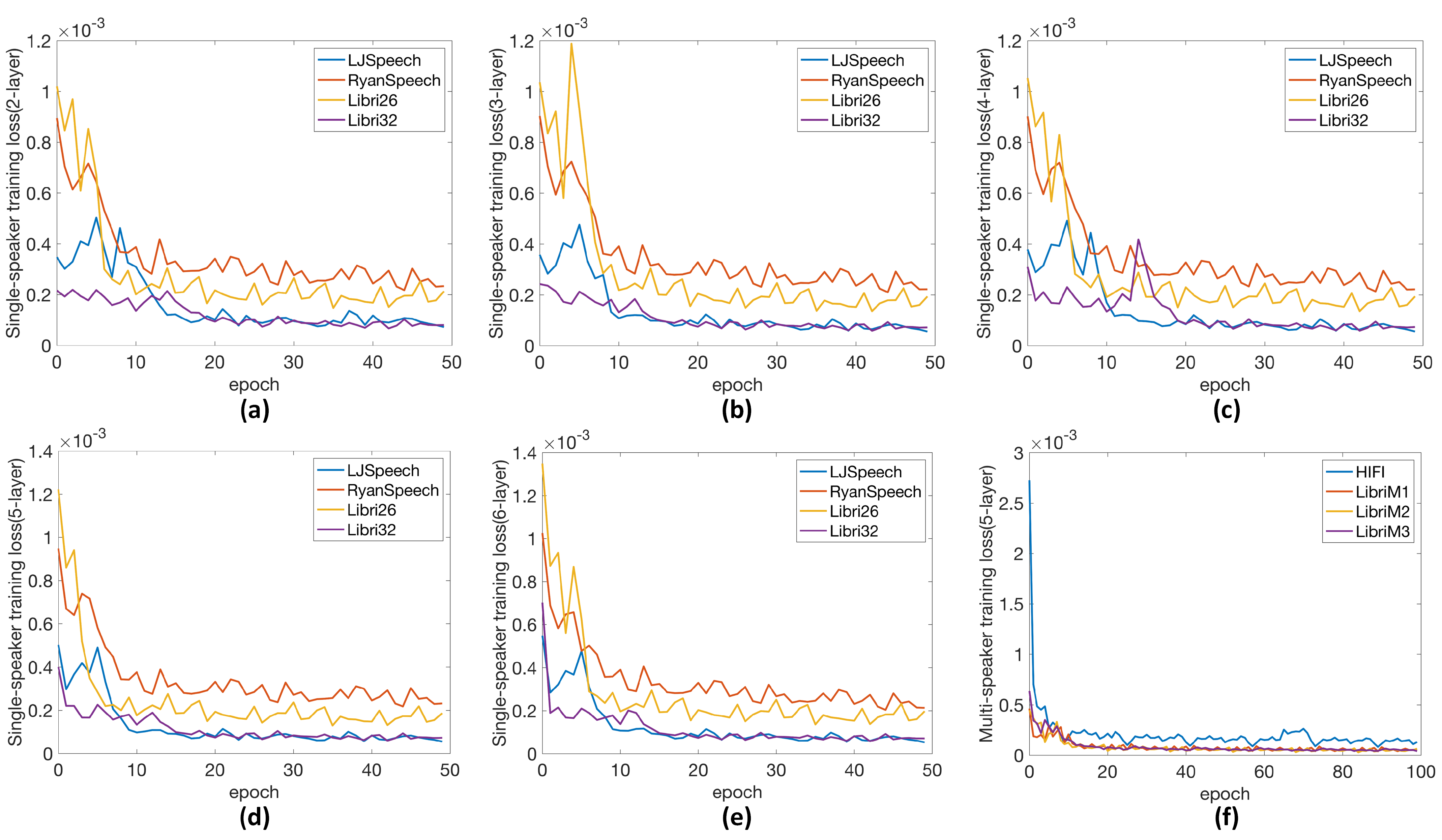
The training loss intuitively reflects the proposed models’ learning ability and convergence degree throughout each epoch. The training losses of models with different LSTM layers trained on four different datasets are shown in Figure 3.

To prevent overfitting during the training of the models, the early stopping regularisation method was used, with the patience value set to five. Two more experiments were conducted to validate the model’s generalisation capability:

• Each trained model was subjected to a series of speech inpainting tests on ten speech signals that were entirely independent of its own dataset. The restored speech signals consistently exhibited good MOSs and listening quality across various gap lengths.
• In order to further validate the generalisation capability, we conducted additional tests to examine the models by training them on a specific dataset and applying them to completely different datasets. In this experiment, a model was first trained on a dataset consisting of only female/male voices, and the model was then applied to restore male/female speech signals from completely different datasets. The inpainting results also demonstrated high MOSs and listening quality across various gap lengths.

As a result, we can reasonably state that no overfitting occurred during the models’ training process and the models generalised well on all the different datasets used in the experiment.

5.2. Inpainting Performance with Different Numbers of LSTM Layers

To examine the inpainting performance of different numbers of LSTM layers on the different single-speaker datasets, we calculated two types of average MOSs for different gap lengths, as shown in

Table 7. Average MOSs for different gap lengths and LSTM layers across four single-speaker datasets (NB).

Dataset	Bandwidth	LSTM Layers	Gap Length (ms)
			20	40	50	100	200	500	1000
LJSpeech	NB	2	4.17	3.96	3.92	3.84	3.71	3.27	2.69
		3	4.15	3.91	3.88	3.80	3.66	3.17	2.56
		4	4.14	3.95	3.92	3.79	3.67	3.21	2.59
		5	4.16	3.96	3.92	3.83	3.67	3.19	2.57
		6	4.10	3.91	3.86	3.77	3.62	3.13	2.49
RyanSpeech	NB	2	4.08	3.94	3.89	3.74	3.48	3.02	2.52
		3	4.15	4.00	3.94	3.74	3.53	3.07	2.56
		4	4.11	3.96	3.91	3.73	3.52	3.03	2.54
		5	4.07	3.91	3.85	3.68	3.43	2.92	2.44
		6	4.13	3.97	3.90	3.73	3.48	3.01	2.48
Libri_26	NB	2	4.29	4.15	4.10	3.90	3.72	3.25	2.68
		3	4.25	4.13	4.10	3.93	3.75	3.29	2.76
		4	4.25	4.14	4.11	3.92	3.77	3.30	2.78
		5	4.29	4.17	4.14	3.98	3.80	3.37	2.86
		6	4.24	4.12	4.09	3.89	3.71	3.22	2.67
Libri_32	NB	2	4.26	4.09	4.03	3.92	3.66	3.21	2.75
		3	4.29	4.07	4.02	3.88	3.64	3.17	2.69
		4	4.24	4.06	4.01	3.84	3.63	3.19	2.70
		5	4.24	4.06	4.00	3.85	3.61	3.14	2.66
		6	4.25	4.10	4.04	3.91	3.68	3.21	2.74

and

Table 8. Average MOSs for different gap lengths and LSTM layers across four single-speaker datasets (WB).

Dataset	Bandwidth	LSTM Layers	Gap Length (ms)
			20	40	50	100	200	500	1000
LJSpeech	WB	2	4.08	3.89	3.88	3.77	3.55	3.00	2.29
		3	4.02	3.86	3.82	3.70	3.47	2.89	2.21
		4	4.03	3.85	3.81	3.69	3.44	2.89	2.21
		5	4.13	3.94	3.89	3.74	3.52	2.94	2.27
		6	4.03	3.88	3.83	3.71	3.46	2.85	2.13
RyanSpeech	WB	2	4.10	3.99	3.93	3.78	3.49	2.90	2.29
		3	4.17	4.01	3.94	3.81	3.50	2.92	2.32
		4	4.12	3.97	3.92	3.78	3.50	2.89	2.27
		5	4.09	3.96	3.90	3.78	3.47	2.87	2.26
		6	4.15	4.01	3.94	3.81	3.50	2.89	2.25
Libri_26	WB	2	4.26	4.08	4.03	3.82	3.60	3.04	2.36
		3	4.18	4.04	4.00	3.80	3.60	3.06	2.42
		4	4.22	4.08	4.03	3.83	3.62	3.07	2.43
		5	4.25	4.09	4.02	3.87	3.62	3.09	2.44
		6	4.20	4.07	4.01	3.82	3.60	3.04	2.39
Libri_32	WB	2	4.33	4.11	4.05	3.94	3.72	3.17	2.53
		3	4.33	4.12	4.07	3.94	3.72	3.17	2.57
		4	4.28	4.11	4.06	3.92	3.70	3.13	2.49
		5	4.28	4.10	4.05	3.92	3.72	3.15	2.55
		6	4.30	4.11	4.07	3.95	3.73	3.15	2.54

.

It can be observed in Table 7 that the two-layer LSTM model performed well across all gap lengths on the LJSpeech dataset. Meanwhile, on the RyanSpeech dataset, the performance of the three-layer LSTM model was better compared to the other models. Notably, on the Libri_26 dataset, the five-layer LSTM model achieved the highest MOSs across all gap lengths and datasets. In the case of the Libri_32 dataset, the six-layer LSTM model exhibited marginally superior performance compared to the two-layer LSTM model, although the difference was not statistically significant.

In Table 8, the results show that on the LJSpeech dataset, the two-layer LSTM model achieved higher average MOSs for gap lengths greater than or equal to 100 ms, whereas the five-layer LSTM model performed better when the gap length was less than 100 ms. Similar results can be observed for the RyanSpeech and Libri_26 datasets in Table 7. However, on the Libri_32 dataset, the three-layer LSTM model achieved the highest MOSs across all datasets.

In summary, it was observed that, for each model with different LSTM layers, the average MOS decreased as the gap length increased. Across the different datasets, the model that obtained the highest average MOS varied. However, the differences among the five LSTM models were not significant, with only minor fluctuations. These slight differences in performance emphasise the impact of model architecture and training datasets on the performance of speech inpainting, which means that it is important to customise the model architecture according to different datasets and inpainting requirements.

5.3. Inpainting Performance Based on Frequency Analysis

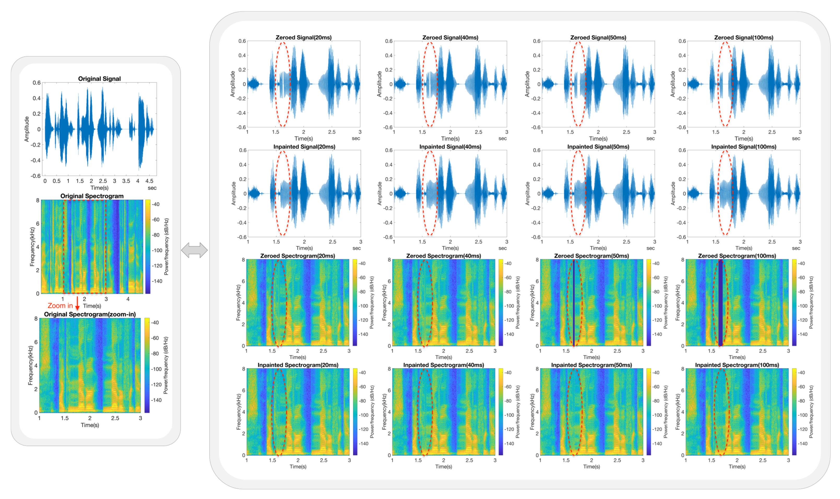
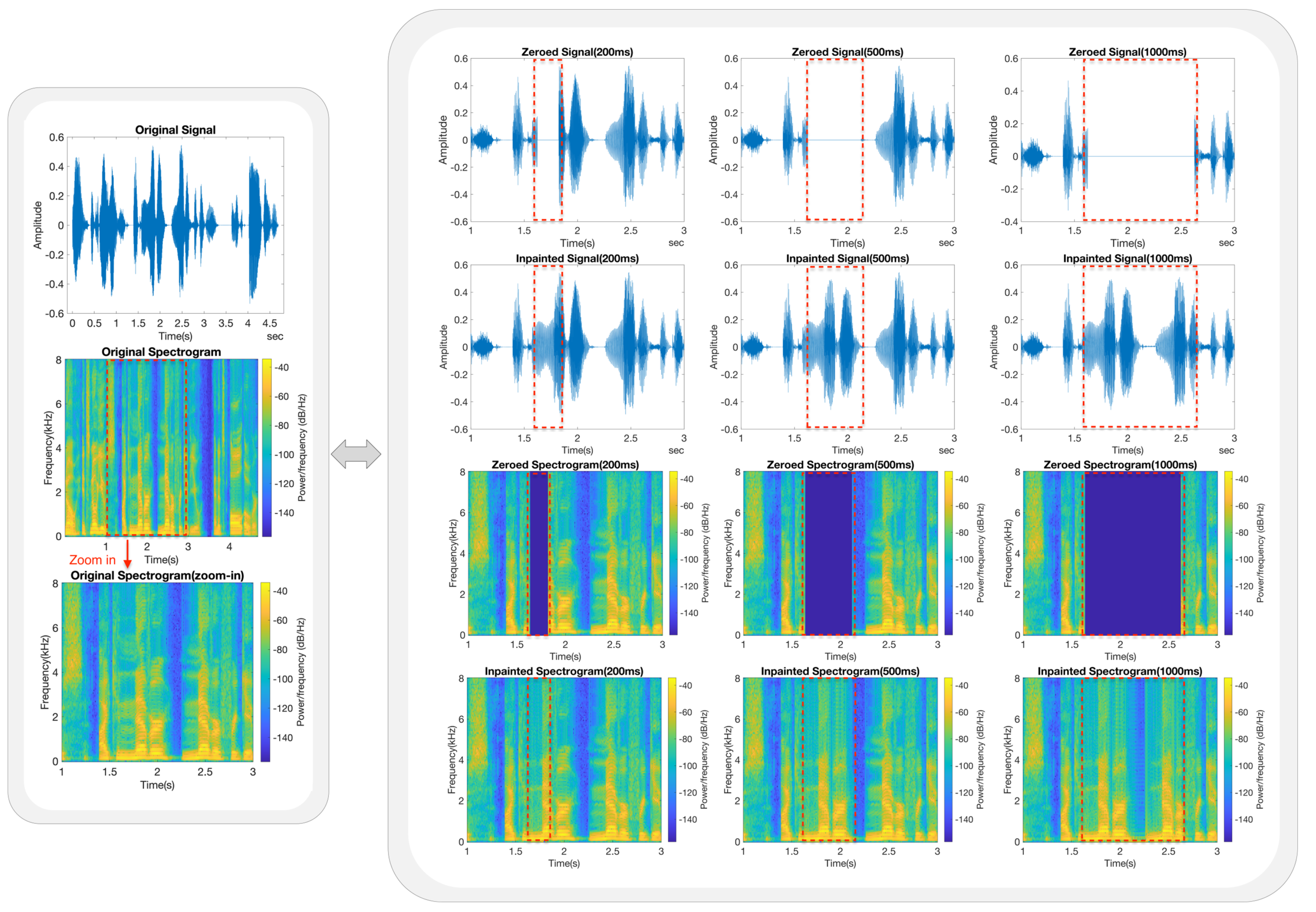
In order to provide an in-depth analysis of the inpainting performance, the frequency analysis method [33] was employed to analyse the spectrogram of the speech signals. The test speech signal was selected from the RyanSpeech dataset, with a duration of 4.7 s, and the gaps started from 1.62 s and lasted for 20 ms, 40 ms, 50 ms, 100 ms, 200 ms, 500 ms, and 1000 ms. A five-layer LSTM model was used to restore the missing speech samples.

As can be seen in Figure 4 and Figure 5, each figure consists of two zones: one on the left and the other on the right. The left side of each figure shows the time-domain waveform, spectrogram, and zoomed-in spectrogram (1.0–3.0 s on the x-axis) from top to bottom. The right side shows the time-domain waveforms and corresponding spectrograms of the zeroed and inpainted speech signals from top to bottom.

It should be noted that except for the original signal and the original spectrogram in the left zone, all the subfigures show the same zoomed-in range of the x-axis (1.0–3.0 s) in order to facilitate a more intuitive comparison between the original and inpainted signals in the frequency domain.

As shown in Figure 4 and Figure 5, all the inpainted waveforms in the time domain follow the trend of the original signal throughout the entire gap length with sufficient accuracy. The predicted waveform envelope of the inpainted signal has extremely high accuracy compared to that of the original signal. In terms of the amplitude, there was only minimal loss, which can be considered negligible. In order to decrease the potential discrepancies caused by objective indicators in perceiving the quality of inpainted speech signals, we conducted subjective listening tests on the inpainted speech signals. During the tests, the inpainted signals revealed clear and highly recognisable characteristics, which led to a high value of the average MOS. The inpainted speech clips and the average MOSs are available at https://haohan-shi.github.io/ (accessed on 9 February 2024).

5.4. Inpainting Performance on Multi-Speaker Datasets

Similar analytic procedures were applied to the multi-speaker datasets, where we exclusively trained a five-layer LSTM model to examine the inpainting performance.

Table 9. Average MOSs of the five-layer LSTM models across four multi-speaker datasets for different gap lengths (NB and WB).

Dataset	Bandwidth	LSTM Layers	Gap Length (ms)
			20	40	50	100	200	500	1000
HIFI	NB	5	4.13	4.04	4.00	3.86	3.58	3.09	2.39
	WB		4.04	3.94	3.84	3.74	3.42	2.77	2.07
LibriM1	NB	5	4.19	4.03	3.98	3.86	3.76	3.34	2.87
	WB		4.18	4.07	4.02	3.85	3.71	3.19	2.57
LibriM2	NB	5	4.12	4.00	3.96	3.80	3.59	3.13	2.60
	WB		4.09	4.00	3.99	3.82	3.52	2.94	2.28
LibriM3	NB	5	4.09	3.86	3.81	3.72	3.44	3.03	2.46
	WB		3.70	3.60	3.57	3.45	3.21	2.74	2.13

shows the average MOSs of the five-layer LSTM models across the four multi-speaker datasets for different gap lengths, comparing the original and inpainted speech signals in both NB and WB scenarios. Similar results can be observed across the four multi-speaker datasets, where the average MOS decreased as the gap length increased in both NB and WB scenarios. For the LibriM1 and LibriM2 datasets, when the gap length was less than or equal to 200 ms, the fluctuation in the average MOS caused by different bandwidths for the same dataset was relatively minor. However, the fluctuation began to increase when the gap length was greater than 200 ms. For the HIFI and LibriM3 datasets, the fluctuation in the average MOS caused by different bandwidths across all gap lengths in the same dataset was subtle.

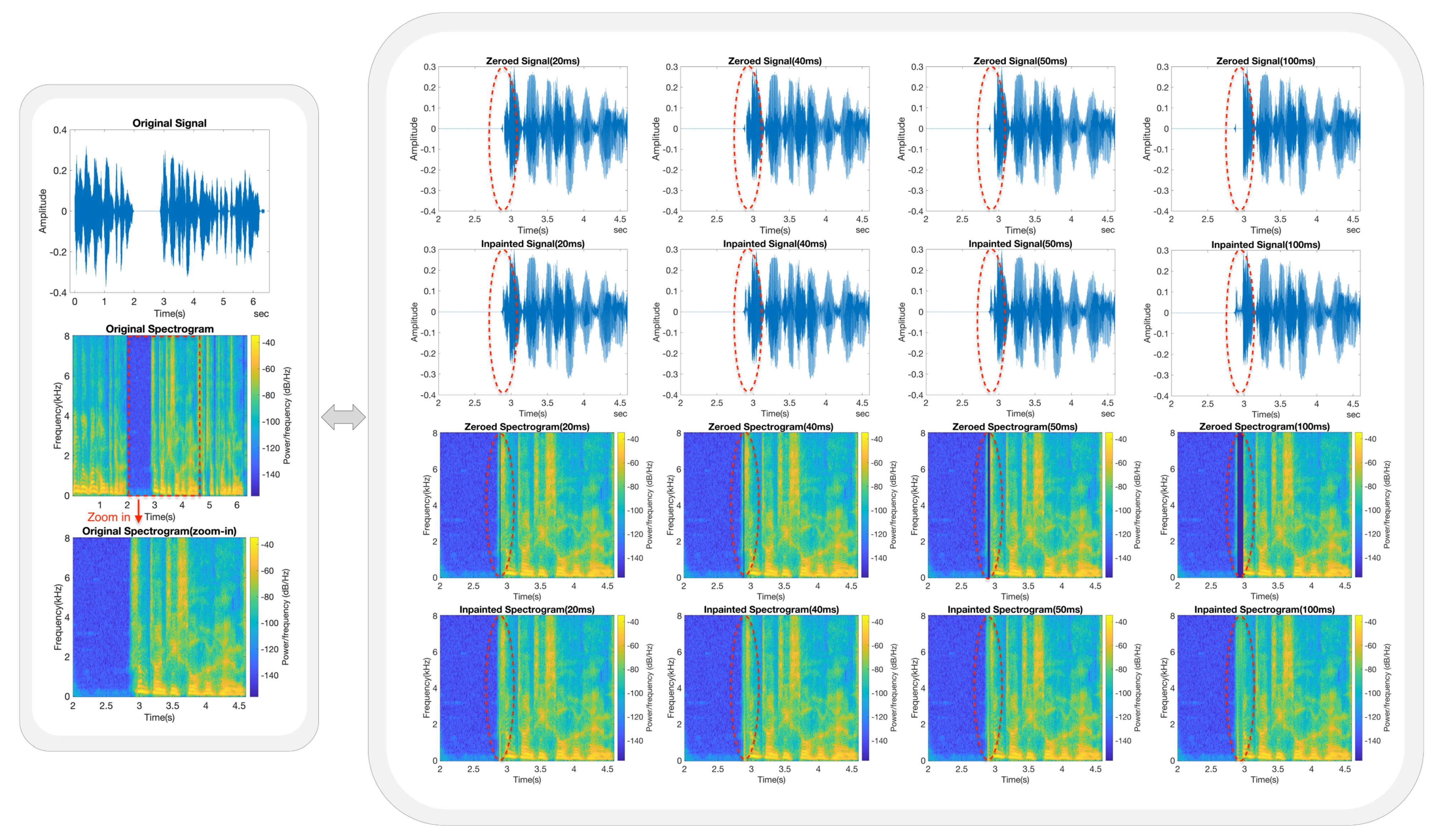
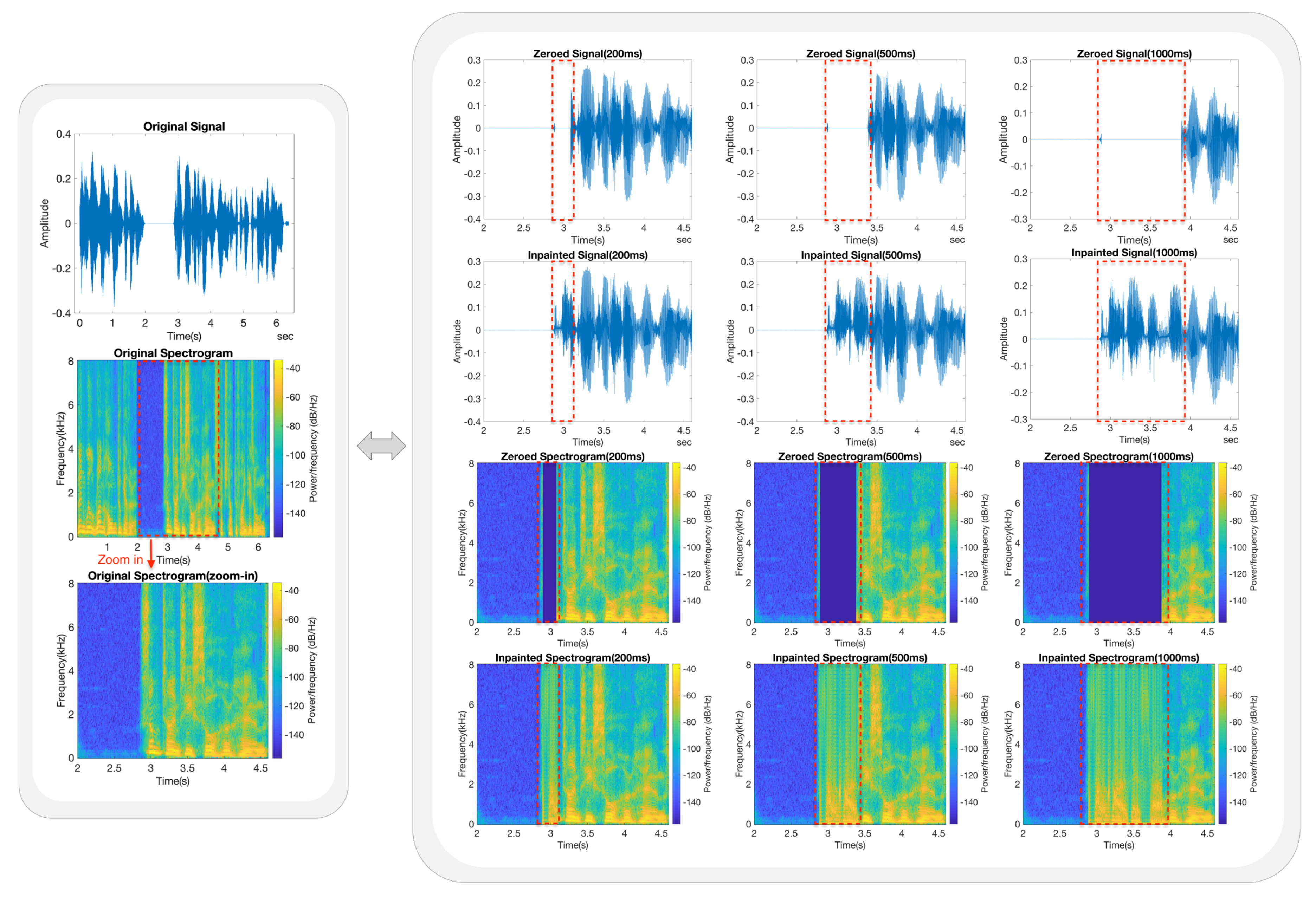
The same frequency analysis procedure was also employed for the multi-speaker datasets. In this case, we selected a test speech signal from the HIFI dataset. The duration of the original signal was 6.38 s, and the gaps started from 2.88 s and lasted for 20 ms, 40 ms, 50 ms, 100 ms, 200 ms, 500 ms, and 1000 ms, respectively. A five-layer LSTM model was used to restore the missing speech samples. In Figure 6 and Figure 7, the layout of each figure is the same as that used previously, with the only difference being that the corresponding zoomed-in range of the x-axis is now 2.0–4.6 s.

In Figure 6 and Figure 7, it can be observed that all the inpainted waveforms in the time domain follow the trend of the original signal throughout the entire gap length with acceptable accuracy. Compared with the original signal, the envelope of the inpainted speech signal follows the shape of the original signal, but with significant losses in amplitude.

We also subjectively tested the listening quality of the inpainted speech signals, as they can offer a basic understanding of the expressed meaning. In contrast to the single-speaker dataset, the restored speech signals in the multi-speaker dataset exhibited reduced clarity and recognisability features. This variation was reflected in the slightly lower average MOSs in both NB and WB scenarios. The inpainted speech clips and the average MOSs are available at https://haohan-shi.github.io/ (accessed on 9 February 2024).

In comparison to the single-speaker model, the multi-speaker model exhibited acceptable inpainting results in the frequency band below 2.0 kHz but with losses in amplitude. In the higher frequency range above 2.0 kHz, the accuracy of the model was low, and the predicted spectrogram blocks were repetitive and oscillatory in the frequency domain, leading to noisy inpainted speech signals with lower perceived quality compared to the single-speaker LSTM models.

5.5. Comparison with Other Algorithms

The performance of the proposed inpainting method was compared with four state-of-the-art algorithms in the literature, including Context-Encoder [22], SpeechPainter [27], Audio-Visual [31], and TF-Masks [23]. The comparison results are listed in

Table 10. Comparison of MOSs between the proposed method and other algorithms.

Method	Gap Length (ms)	MOS (NB)	MOS (WB)
Context-Encoder [22]	64/128	4.02/3.57	3.95/3.48
SpeechPainter [27]	750–1000	\	3.48 ± 0.06
Audio-Visual (A+V+MTL) [31]	100/200/400/800/1600	\	4.10/3.82/3.43/2.49/1.56
TF-Masks-informed (Avg. of 3 intrusions) [23]	100/200/300/400	\	3.20/2.57/2.09/1.78
TF-Masks-blind (Avg. of 3 intrusions) [23]	100/200/300/400	\	3.17/2.75/2.46/2.21
Proposed method (single-speaker)	20/40/50/100 /200/500/1000	4.19/4.03/3.98/3.84 /3.64/3.17/2.64	4.18/4.02/3.97/3.82 /3.58/3.01/2.36
Proposed method (multi-speaker)	20/40/50/100 /200/500/1000	4.14/3.98/3.94/3.81 /3.60/3.15/2.58	4.01/3.91/3.86/3.72 /3.47/2.91/2.27

.

The Context-Encoder, originally designed for inpainting music signals, was adapted to our established speech datasets. We conducted MOS tests for two gap lengths, specifically 64 ms and 128 ms, considering both NB and WB scenarios. Human raters were used in [27] for accessing the MOS, we categorised it under MOS(WB). The studies by [23,31] only exhibited the Perceptual Evaluation of Speech Quality (PESQ) scores to indicate the quality of the inpainted signals. To facilitate comparison, we employed a mapping method to convert the raw PESQ scores into MOS(WB) [50].

The results indicate that our methods outperformed the TF-Mask method across all gap lengths. In the case of the Context-Encoder method, our approaches demonstrated superior performance when the gap length was 128 ms. When the gap length was 64 ms, there were no significant differences in the MOSs for the NB scenario, and they maintained comparable performance for the WB scenario. The SpeechPainter and Audio-Visual methods exhibited slightly higher MOSs compared to our methods. This is because our proposed approaches only used the speech features preceding the gap for inpainting, without utilising any additional information. In contrast, SpeechPainter utilised the entire speech transcripts, whereas the Audio-Visual method combined both speech and visual features, leading to higher MOSs. Nevertheless, it is worth noting that in real-world communication scenarios, there will not always be support and time for additional information (i.e., the transcript) to be considered, particularly when a two-way live conversation is ongoing between communicators. As such, our proposal fills in this gap to greatly enhance the user experience.

5.6. Limitations

When evaluating the performance of the inpainting results across diverse datasets, it was observed that the model achieving the optimal MOS contained a different number of LSTM layers. In the time domain, the proposed models proficiently restored the waveform envelope trends of the lost speech signals; however, a discernible loss in amplitude was observed. As for the frequency domains, it was observed that the proposed models effectively restored the speech signal’s lower frequency range below 2.0 kHz for both single-speaker and multi-speaker datasets with sufficient accuracy. However, the efficacy of the model was limited at higher frequency ranges exceeding 2.0 kHz, especially for the multi-speaker datasets, exhibiting a significant loss in amplitude and introducing more pitch frequencies to the spectrograms. However, the listening quality was still understandable and acceptable.

It is worth mentioning that we only used a compact training dataset built from the RyanSpeech dataset for training and testing during the fine-tuning of the hyperparameters. Subsequently, the optimised hyperparameters were applied to all the other datasets. This means that the optimal hyperparameters based on the RyanSpeech dataset may not be the best-fitting choice for all datasets. To achieve better inpainting performance, fine-tuning for different datasets should be considered. We systematically tested various hyperparameter configurations, including a trial employing the five-layer LSTM model with specific settings: batch size = 512, dropout rate = 0.2, and dropout layers placed after the first and last LSTM layers. Notably, this configuration also achieved ideal inpainting results.

We conducted additional tests to assess the inpainting capability of models trained on specific datasets when applied to different datasets. The inpainting performance exhibited a diverse range of outcomes.

6. Conclusions and Future Work

This study proposed multi-layer LSTM networks for speech inpainting in the time domain. We compared the inpainting performance of the proposed models on different datasets and with different numbers of LSTM layers. We then evaluated the performance under different gap lengths using the MOS and frequency analysis method. Our tests demonstrated that the proposed multi-layer LSTM model can restore up to 1 s of gaps with fair and good perceived quality using features captured only from the time domain. Specifically, for gaps below 500 ms, the recorded MOS can reach 3 to 4 or above, and for gaps between 500 ms and 1s, the MOS can reach 2 to 3 or above. This study confirmed that the multi-layer LSTM model can be effectively used in speech inpainting to restore up to 1 s of gaps while providing sufficiently accurate results.

Our future work will focus on performing speech inpainting for high-quality speech coding in information communication settings.

References

- Adler, A.; Emiya, V.; Jafari, M.G.; Elad, M.; Gribonval, R.; Plumbley, M.D. Audio inpainting. IEEE Trans. Audio Speech Lang. Process. 2011, 20, 922–932. [Google Scholar] [CrossRef]
- Janssen, A.; Veldhuis, R.; Vries, L. Adaptive interpolation of discrete-time signals that can be modeled as autoregressive processes. IEEE Trans. Acoust. Speech Signal Process. 1986, 34, 317–330. [Google Scholar] [CrossRef]
- Oudre, L. Interpolation of Missing Samples in Sound Signals Based on Autoregressive Modeling. Image Process. Line 2018, 8, 329–344. [Google Scholar] [CrossRef]
- Etter, W. Restoration of a discrete-time signal segment by interpolation based on the left-sided and right-sided autoregressive parameters. IEEE Trans. Signal Process. 1996, 44, 1124–1135. [Google Scholar] [CrossRef]
- Lagrange, M.; Marchand, S.; Rault, J.B. Long interpolation of audio signals using linear prediction in sinusoidal modeling. J. Audio Eng. Soc. 2005, 53, 891–905. [Google Scholar]
- Lukin, A.; Todd, J. Parametric interpolation of gaps in audio signals. In Audio Engineering Society Convention 125; Audio Engineering Society: New York, NY, USA, 2008. [Google Scholar]
- Kauppinen, I.; Kauppinen, J.; Saarinen, P. A method for long extrapolation of audio signals. J. Audio Eng. Soc. 2001, 49, 1167–1180. [Google Scholar]
- Kauppinen, I.; Roth, K. Audio signal extrapolation–theory and applications. In Proceedings of the Proc. DAFx, Hamburg, Germany, 26–28 September 2002; pp. 105–110. [Google Scholar]
- Goodman, D.; Lockhart, G.; Wasem, O.; Wong, W.C. Waveform substitution techniques for recovering missing speech segments in packet voice communications. IEEE Trans. Acoust. Speech Signal Process. 1986, 34, 1440–1448. [Google Scholar] [CrossRef]
- Smaragdis, P.; Raj, B.; Shashanka, M. Missing data imputation for spectral audio signals. In Proceedings of the 2009 IEEE International Workshop on Machine Learning for Signal Processing, Grenoble, France, 1–4 September 2009; pp. 1–6. [Google Scholar] [CrossRef]
- Smaragdis, P.; Raj, B.; Shashanka, M. Missing data imputation for time-frequency representations of audio signals. J. Signal Process. Syst. 2011, 65, 361–370. [Google Scholar] [CrossRef]
- Bertalmio, M.; Sapiro, G.; Caselles, V.; Ballester, C. Image inpainting. In Proceedings of the 27th Annual Conference on Computer Graphics and Interactive Techniques, New Orleans, LA, USA, 23–28 July 2000; pp. 417–424. [Google Scholar]
- Godsill, S.; Rayner, P.; Cappé, O. Digital Audio Restoration; Applications of digital signal processing to audio and acoustics; Springer: Berlin/Heidelberg, Germany, 2002; pp. 133–194. [Google Scholar]
- Hochreiter, S.; Schmidhuber, J. Long short-term memory. Neural Comput. 1997, 9, 1735–1780. [Google Scholar] [CrossRef]
- Sanneck, H.; Stenger, A.; Younes, K.B.; Girod, B. A new technique for audio packet loss concealment. In Proceedings of the GLOBECOM’96, 1996 IEEE Global Telecommunications Conference, London, UK, 18–28 November 1996; pp. 48–52. [Google Scholar]
- Bahat, Y.; Schechner, Y.Y.; Elad, M. Self-content-based audio inpainting. Signal Process. 2015, 111, 61–72. [Google Scholar] [CrossRef]
- Lieb, F.; Stark, H.G. Audio inpainting: Evaluation of time-frequency representations and structured sparsity approaches. Signal Process. 2018, 153, 291–299. [Google Scholar] [CrossRef]
- Adler, A.; Emiya, V.; Jafari, M.G.; Elad, M.; Gribonval, R.; Plumbley, M.D. A constrained matching pursuit approach to audio declipping. In Proceedings of the 2011 IEEE International Conference on Acoustics, Speech and Signal Processing (ICASSP), Prague, Czech Republic, 22–27 May 2011; pp. 329–332. [Google Scholar]
- Tauböck, G.; Rajbamshi, S.; Balazs, P. Dictionary learning for sparse audio inpainting. IEEE J. Sel. Top. Signal Process. 2020, 15, 104–119. [Google Scholar] [CrossRef]
- Mokrý, O.; Rajmic, P. Audio Inpainting: Revisited and Reweighted. IEEE/ACM Trans. Audio Speech Lang. Process. 2020, 28, 2906–2918. [Google Scholar] [CrossRef]
- Chantas, G.; Nikolopoulos, S.; Kompatsiaris, I. Sparse audio inpainting with variational Bayesian inference. In Proceedings of the 2018 IEEE International Conference on Consumer Electronics (ICCE), Las Vegas, NV, USA, 12–14 January 2018; pp. 1–6. [Google Scholar] [CrossRef]
- Marafioti, A.; Perraudin, N.; Holighaus, N.; Majdak, P. A context encoder for audio inpainting. IEEE/ACM Trans. Audio Speech Lang. Process. 2019, 27, 2362–2372. [Google Scholar] [CrossRef]
- Kegler, M.; Beckmann, P.; Cernak, M. Deep speech inpainting of time-frequency masks. arXiv 2019, arXiv:1910.09058. [Google Scholar]
- Goodfellow, I.; Pouget-Abadie, J.; Mirza, M.; Xu, B.; Warde-Farley, D.; Ozair, S.; Courville, A.; Bengio, Y. Generative adversarial networks. Commun. ACM 2020, 63, 139–144. [Google Scholar] [CrossRef]
- Ebner, P.P.; Eltelt, A. Audio inpainting with generative adversarial network. arXiv 2020, arXiv:2003.07704. [Google Scholar]
- Marafioti, A.; Majdak, P.; Holighaus, N.; Perraudin, N. GACELA: A generative adversarial context encoder for long audio inpainting of music. IEEE J. Sel. Top. Signal Process. 2020, 15, 120–131. [Google Scholar] [CrossRef]
- Borsos, Z.; Sharifi, M.; Tagliasacchi, M. Speechpainter: Text-conditioned speech inpainting. arXiv 2022, arXiv:2202.07273. [Google Scholar]
- Jaegle, A.; Borgeaud, S.; Alayrac, J.B.; Doersch, C.; Ionescu, C.; Ding, D.; Koppula, S.; Zoran, D.; Brock, A.; Shelhamer, E.; et al. Perceiver io: A general architecture for structured inputs & outputs. arXiv 2021, arXiv:2107.14795. [Google Scholar]
- Vaswani, A.; Shazeer, N.; Parmar, N.; Uszkoreit, J.; Jones, L.; Gomez, A.N.; Kaiser, Ł.; Polosukhin, I. Attention is all you need. Adv. Neural Inf. Process. Syst. 2017, 30. [Google Scholar] [CrossRef]
- Montesinos, J.F.; Michelsanti, D.; Haro, G.; Tan, Z.H.; Jensen, J. Speech inpainting: Context-based speech synthesis guided by video. arXiv 2023, arXiv:2306.00489. [Google Scholar]
- Morrone, G.; Michelsanti, D.; Tan, Z.H.; Jensen, J. Audio-visual speech inpainting with deep learning. In Proceedings of the ICASSP 2021–2021 IEEE International Conference on Acoustics, Speech and Signal Processing (ICASSP), Toronto, ON, Canada, 6–11 June 2021; pp. 6653–6657. [Google Scholar]
- ITU; ITUTP. A Method for Subjective Performance Assessment of the Quality of Speech Voice Output Devices; International Telecommunication Union Std: Geneva, Switzerland, 1994. [Google Scholar]
- Bose, T.; Meyer, F. Digital Signal and Image Processing; John Wiley & Sons, Inc.: Hoboken, NJ, USA, 2003. [Google Scholar]
- Berouti, M.; Schwartz, R.; Makhoul, J. Enhancement of speech corrupted by acoustic noise. In Proceedings of the ICASSP’79, IEEE International Conference on Acoustics, Speech, and Signal Processing, Washington, DC, USA, 2–4 April 1979; Volume 4, pp. 208–211. [Google Scholar]
- Atal, B. Predictive coding of speech at low bit rates. IEEE Trans. Commun. 1982, 30, 600–614. [Google Scholar] [CrossRef]
- Moliner, E.; Välimäki, V. Diffusion-Based Audio Inpainting. arXiv 2023, arXiv:2305.15266. [Google Scholar]
- Zaremba, W.; Sutskever, I.; Vinyals, O. Recurrent neural network regularization. arXiv 2014, arXiv:1409.2329. [Google Scholar]
- Ito, K.; Johnson, L. The LJ Speech Dataset. 2017. Available online: https://keithito.com/LJ-Speech-Dataset/ (accessed on 9 February 2024).
- Bakhturina, E.; Lavrukhin, V.; Ginsburg, B.; Zhang, Y. Hi-Fi Multi-Speaker English TTS Dataset. arXiv 2021, arXiv:2104.01497. [Google Scholar]
- Zandie, R.; Mahoor, M.H.; Madsen, J.; Emamian, E.S. Ryanspeech: A corpus for conversational text-to-speech synthesis. arXiv 2021, arXiv:2106.08468. [Google Scholar]
- Panayotov, V.; Chen, G.; Povey, D.; Khudanpur, S. Librispeech: An asr corpus based on public domain audio books. In Proceedings of the 2015 IEEE International Conference on Acoustics, Speech and Signal Processing (ICASSP), South Brisbane, QUE, Australia, 19–24 April 2015; pp. 5206–5210. [Google Scholar]
- Bengio, Y. Practical recommendations for gradient-based training of deep architectures. In Neural Networks: Tricks of the Trade: Second Edition; Springer: Berlin/Heidelberg, Germany, 2012; pp. 437–478. [Google Scholar]
- Enhanced Voice Services Codec for LTE, 3GPP TR 26.952. 2014. Available online: https://www.3gpp.org/news-events/3gpp-news/evs-news (accessed on 9 February 2024).
- Codec for Enhanced Voice Services (EVS); General Overview. Technical Specification (TS) 26.441 3rd Generation Partnership Project (3GPP). 2018. Available online: https://www.etsi.org/deliver/etsi_ts/126400_126499/126441/15.00.00_60/ts_126441v150000p.pdf (accessed on 9 February 2024).
- Extended Reality (XR) in 5G. Technical Specification (TS) 26.928 3rd Generation Partnership Project (3GPP). 2020. Available online: https://www.etsi.org/deliver/etsi_tr/126900_126999/126928/16.00.00_60/tr_126928v160000p.pdf (accessed on 9 February 2024).
- P.862: Revised Annex A—Reference Implementations and Conformance Testing for ITU-T Recs P.862, P.862.1 and P.862.2. 2005. Available online: https://www.itu.int/rec/T-REC-P.862-200511-I!Amd2/en (accessed on 9 February 2024).
- Patro, S.; Sahu, K.K. Normalization: A preprocessing stage. arXiv 2015, arXiv:1503.06462. [Google Scholar] [CrossRef]
- Lehmann, E.L.; Casella, G. Theory of Point Estimation; Springer Science & Business Media: Berlin/Heidelberg, Germany, 2006. [Google Scholar]
- Kingma, D.P.; Ba, J. Adam: A method for stochastic optimization. arXiv 2014, arXiv:1412.6980. [Google Scholar]
- P.862.1: Mapping Function for Transforming P.862 Raw Result Scores to MOS-LQO. 2003. Available online: https://www.itu.int/rec/T-REC-P.862.1/en (accessed on 9 February 2024).
Figure 1.
LSTM cell structure.
Figure 2.
The inpainting process and neural network structure of the proposed speech inpainting model.
Figure 3.
Training losses of the proposed speech inpainting models on single-speaker datasets with different numbers of LSTM layers: (a–e) speech inpainting models with two to six LSTM layers, respectively; (f) the 5–layer LSTM model trained on four multi–speaker datasets.
Figure 4.
Frequency analysis for gap lengths less than 100 ms. The gaps start at 1.62 s and last for 20 ms, 40 ms, 50 ms, and 100 ms, respectively, corresponding to the first to fourth columns on the right side of the figure. The zoomed–in and gap areas are marked with red dashed lines.
Figure 5.
Frequency analysis for gap lengths greater than 100 ms. The gaps start at 1.62 s and last for 200 ms, 500 ms, and 1000 ms, respectively, corresponding to the first to third columns on the right side of the figure. The zoomed–in and gap areas are marked with red dashed lines.
Figure 6.
Frequency analysis for gap lengths less than 100 ms. The gaps start at 2.88 s and last for 20 ms, 40 ms, 50 ms, and 100 ms, respectively, corresponding to the first to fourth columns on the right side of the figure. The zoomed–in and gap areas are marked with red dashed lines.
Figure 7.
Frequency analysis for gap lengths greater than 100 ms. The gaps start at 2.88 s and last for 200 ms, 500 ms, and 1000 ms, respectively, corresponding to the first to third columns on the right side of the figure. The zoomed–in and gap areas are marked with red dashed lines.