

Mechanical Properties of Wood: A Review
by
 , , and
Francisco Arriaga
1,*,
Xiping Wang
2,
Guillermo Íñiguez-González
1,
Daniel F. Llana
1,
Miguel Esteban
1 and
Peter Niemz
3 1
Timber Construction Research Group, Department of Forest and Environmental Engineering and Management, MONTES (School of Forest Engineering and Natural Resources), Universidad Politécnica de Madrid, 28040 Madrid, Spain
2
Forest Products Laboratory, USDA Forest Service, Madison, WI 53726, USA
3
Chair of Wood Physics, Department of Civil, Environmental and Geomatic Engineering, ETH Zürich, 8092 Zürich, Switzerland
*
Author to whom correspondence should be addressed.
Forests 2023, 14(6), 1202; https://doi.org/10.3390/f14061202
Submission received: 11 April 2023
/
Revised: 22 May 2023
/
Accepted: 2 June 2023
/
Published: 9 June 2023
(This article belongs to the Special Issue Reviews on Structure and Physical and Mechanical Properties of Wood)
Abstract
:The use of wood in construction requires knowledge of the mechanical properties and the particularities that wood presents in comparison with other materials used for structural purposes such as steel, concrete, brick, or stone. The introduction mentions the environmental advantages that justify the use of wood today. The orthotropy of wood is one of the differentiating characteristics that must be taken into account when studying its behaviour. The determination of the properties of wood is then addressed from a historical perspective and the differentiation is made between the properties of small clear wood (defect-free timber) and structural timber. The timber grading systems (visual and mechanical grading) and the non-destructive techniques that currently prevail are explained. Finally, the factors that influence the mechanical properties, such as duration of the load, moisture content, quality, temperature, and the effect of size are explained. The objective of this work is to provide an overview of the current knowledge on the mechanical properties of wood, based mainly on published articles and European and North American standards, including historical references to the beginnings and current trends in this field.
1. Introduction: Wood as a Sustainable Building Material and the Recent Evolution of Wooden Construction
1.1. Timber Construction Is Modern, Sustainable, and Efficient
Even those without technical knowledge would identify a good building material as being one which is efficient, economical, durable, resistant, flexible, or comfortable. In more recent times, the characteristic of sustainability has gained particular importance. Wood has been used as a structural material for millennia, ever since mankind first discovered the possible uses of this natural product. Although other, seemingly superior innovative solutions have substituted many of the historical uses of wood, it is now regaining the prominence that it once had.
Furthermore, the employment of wood can also be positive for forests as long as it is carried out rationally. In America, Europe, and other areas in which sustainability criteria are incorporated into modern forest management techniques, the forested area is increasing despite the rising demand for wood. The EU-28 produces 110 million m3 of sawn timber per year [1], which equates to enough wood being produced every 8 s to build a three-person apartment, for example.
Wood is far from being an obsolete material. In fact, through technology, standardisation, and training, it has become a cutting-edge material, fully incorporated into the regulations throughout almost all the world. Standardisation efforts in many countries over recent decades have contributed towards wood being considered a ‘modern’ material, adapted to the strictest safety, industrial and market requirements. Acoustic properties, durability, and fire resistance are important aspects that are no longer baseless clichés and which can be achieved by adopting the appropriate technical specifications. Wood products have been developed in competitive and effective formats and dimensions, including Glued Laminated Timber (glulam), Cross Laminated Timber (CLT), or Laminated Veneer Lumber (LVL), among others, providing robust mechanical performance. Wood has brought together the most advanced parametric design, numerical control, and BIM technology. Moreover, the curricula in universities now incorporate extensive technical training in timber construction.
Building with wood does not pollute the environment. In a sector responsible for high greenhouse gas emissions, investors have turned their attention to wood and forests as carbon sinks. Thanks to photosynthesis (which is free!) 1 m3 of wood, weighing about 600 kg, fixes approximately 1.5 t of CO2. A simple comparison of the consequences of using different materials with equal performance for a generic beam in a building (5.0 m span and 3 kN/m load) gives an irrefutable result, Figure 1.
A more complete comparison over a real build also provides clear results in terms of the sustainability of wood as a natural resource. In a building in Växjö, Sweden, with seven wooden floors built on a cast concrete base (Limnologen building), each 125 m2 apartment needs about 28 m3 of wood. If a spruce forest produces approximately 4 m3/ha/year of wood, according to the current silvicultural and harvesting approach in Europe, each apartment requires about 7 ha of forest. For a service life of 50 years and a forest rotation period of 50 years, the area required to maintain this dwelling would be 0.14 ha. If the entire European population lived in this type of housing (750 million population and an average of 3 inhabitants per apartment), about 35 × 106 ha of forest would be needed, which represents 20% of the European forest [3].
Wood is as efficient as steel or concrete. As regards structural efficiency, it should be borne in mind that the determining factor in the dimensioning of a wooden structure is usually the modulus of elasticity (MOE). Thus, a representative comparison of the structural efficiency must be based on the MOE relative to the quantity of material, or density. On this basis, comparing the use as a beam and potential bending, standard structural wood would be comparable to steel, titanium, or aluminium. As a column, wood is comparable to carbon fibre composite, and as a panel, it is superior to all these materials, even if buckling is considered [4]
Table 1 shows this comparison between different materials and common timber structural products (coniferous sawn timber, C24 Strength Class according to EN 338 European standard), or high strength products (LVL, equivalent to a C40 Strength Class according to EN 338 European standard) under Ultimate Limit State (ULS) and characteristic values of the mechanical properties, or Serviceability Limit State (SLS) and average values.
1.2. Sustainability Assessment as a Requirement
There are no buildings that have zero impact. During the design stage, the impact of buildings can be measured in order to try to mitigate it. In 2015, the UN established the 17 Sustainable Development Goals (SDGs) [5], nine of which are directly related to construction.
From the point of view of sustainability, the result of any comparison between different construction systems and materials is always favourable towards the timber. The following example is based on the evaluation of the Product Environmental Footprint (PEF) of a real house, according to the recommendations of the European Commission [6]. The subject of the analysis was a 247 m2 detached house built in 2019 close to Madrid (Spain), which was representative of prevailing wooden construction types (mixed CLT panels for vertical and horizontal structures, and glulam beams for the roof structure). The project is based on sustainability and bioconstruction criteria, so the result is a high-efficiency building, approximating the Passive House standard, although without certification.
The study embraces the house as a whole, its use over 50 years, and its demolition, analysing 16 impact categories [7]. Regarding the ‘use’ phase, the energy demand and its impacts have been calculated, including maintenance and repairs of the building [8].
Regarding the construction phase, the critical points in terms of impacts centre on the foundations and on the timber structure. The main impacts produced by foundations are related to concrete (during the production of cement and aggregates) and steel (rebar production). In the case of the timber structure, the manufacturing of CLT and glulam beams are responsible for most of the impacts, together with the erection crane and transport. In terms of the overall impacts, the percentage due to the foundations and concrete structure (37%) far exceeds that of the timber structure (9%) [9].
As a result of this study, several considerations can be identified which must be taken into account in the design:
- -
- Reducing the use of concrete and cement as far as possible.
- -
- Reducing the consumption of water.
- -
- Use of timber
- -
- Use of local (zero-mile), easily recyclable materials where possible.
- -
- Improved energy efficiency and implement sustainable sources of energy (photovoltaic panels).
- -
- The design to reduce maintenance costs and allow reutilisation.
1.3. Trends in Timber Construction
In many countries, timber construction has been well established over the years or even centuries, but in others, timber is a relatively new material for construction purposes. The tendency in recent years has been strongly influenced by the development of CLT. Moreover, CLT has opened the gate for other timber materials and construction systems.
Tendencies currently focus on the interest in developing new timber products and wooden construction systems, optimizing these products and systems for structural use. Hence, while small constructions and single, timber-framed houses are relatively common, CLT construction technology has begun to appear on the market over recent years, not only for small and medium size constructions but also for high buildings. This evolution has led to mixed systems, examples of this tendency being Mjøstårnet (Brumunddal, Norway), Hoho Wien (Wien, Austria), Sara Cultural Centre (Skellefteå, Sweden), García Márquez Library (Barcelona, Spain), UBC residence (Vancouver, BC, Canada) or Carbon 12 (Portland, OR, USA) among many others from all over the world.
The benefits of timber construction systems cannot be considered purely in terms of environmental impacts, i.e., reducing the carbon footprint, but also in social and economic terms. In general, the cost of timber solutions tends to be slightly higher than other common systems, such as concrete, bricks, or steel. Some authors put the increased cost at around 10% although it should also be noted that the usable area in timber buildings can be around 7% greater [10]. Depending on the cost of the buildable area available in many cities, it could be of interest to undertake a detailed cost analysis. Another advantage of wooden construction is the comparatively short execution time required. For example, in the case of a medium-rise building for residential use, the total execution time can be 2 or 3 months shorter than for steel or concrete. A timber build is also lighter, so the foundations are simple and less costly. The physical properties of wood contribute to avoiding thermal bridging, as well as to improving the hygro-thermal and acoustic performance of the building for the dwellers and workers. Finally, the rapid, relatively noise-free erection of the structure accompanied by the ‘friendly’ smell of wood, leads to a positive perception of the building environment by the local population. In short, many factors have contributed to sparking the interest of designers, architects, and engineers in timber construction for many kinds of buildings, especially in cities.
2. Orthotropic Properties of Wood and Main Influencing Factors
2.1. Structure of Wood
The structure of wood can be divided into three levels: macrostructure, microstructure, and sub-microstructure, Figure 1. The properties of wood are determined by all structural characteristics [11,12,13,14,15,16]. The content of this section is a brief summary of the relationships between the structure and properties of wood.
Essential structural features at macroscopic, microscopic, and sub-microscopic scales are detailed in the following selected examples:
Macroscopic scale: the slope of grain, annual ring orientation, sapwood and heartwood, juvenile and mature wood, the width of growth rings, the proportion of latewood, and reaction wood.
Microscopic scale: tissue proportions, tissue arrangement, tissue dimension, fibre length, fibre wall thickness, the influence of the wood rays on mechanical properties and swelling, cell wall proportion as a whole, and reaction wood.
Sub-microscopic scale: the thickness of cell wall layers, microfibril orientation (in S2 layer), and lignification of cell wall layers.
2.2. Structure-Property Relationship (Small Clear Specimens)
The structure of wood is crucial in determining the properties on all three structural levels, Figure 2. At the macrostructural level, there are clear influences of density, grain angle, and annual ring orientation (ring angle). In particular, bulk density is a dominant influencing variable, Figure 2III.
However, at the cell wall level, there is also a clear influence of the microfibril angle (MFA) on the mechanical properties (modulus of elasticity, strength) as well as the swelling and shrinkage behaviour present [14,17,18,19]. A very good overview of research on MFA is given in [14].
At the component level (lumber, glulam), wood properties depend on loading direction, exhibiting large variability between boards (caused by growth conditions, the position of the board in the trunk during cutting).
Figure 2.
Main structural parameters influencing the wood properties ([15,20]. (I) Cell wall structure: longitudinal tension of yew and spruce fibres calculated on the cell wall cross-sectional area (cw), without a lumen. (a) Stress-strain diagram; (b) Ultimate stress; (c) Strain at break; (d) Modulus of elasticity. Microfibril angle: spruce 0–5°, yew 15–20° ([16] (Courtesy of D. Keunecke). (II) Microstructure. (III) Macrostructure. (IV) The relationship between density and bending strength using material parameters from the literature on 103 wood species [15] (courtesy of Carl Hanser Verlag GmbH & Co. KG, Munich, Germany); data from [21].

2.3. Orthotropic Mechanical Properties of Wood
The mechanical properties of wood and wood-based materials (modulus of elasticity, shear modulus, and Poisson’s ratio) present elastic and inelastic behaviour (time and MC change dependent). These properties are viscoelastic because the behaviour is time-dependent and manifests itself in creep and relaxation. Furthermore, they are considered mechano-sorptive properties, which reflect the behaviour under simultaneous load and humidity change as well as plastic properties, which appear as permanent deformation (e.g., plastic components of creep deformation, plastic deformation under load above the limit of proportionality). The orthotropy is described below only for the elastic properties, although it also applies to inelastic properties and strength.
2.3.1. Elastic Law and Stress-Strain Diagram (Hooke’s Law)
There is a linear relationship between stress and strain in ideal elastic bodies (Hooke’s Law). A solid body becomes longer in the case of tensile load and shorter under compression, while shear stresses produce angle distortion, Figure 3. After release, the deformation of an ideal elastic body completely regresses, Figure 4a. This applies as long as the mechanical stress is below the proportional limit. The proportional limit varies with the moisture content of the wood. It is about 50%–60% of the maximum stress at tensile load under normal climatic conditions. The modulus of elasticity (Young’s modulus) is calculated from the slope of the straight line in the stress-strain diagram. Above the proportional limit, plastic deformation occurs. Plastic strain under tension is very limited but not under compression. In directions parallel and perpendicular to the fibre, ultimate strain under tensile load is low (0.7%–1%). Perpendicular to the fibre, compressive loading above the proportional limit leads to considerable plastic deformation. Wood can densify to a high degree under compression, in particular in the radial direction, Figure 4b, e.g., spruce from 450 kg/m3 to 1200 kg/m3 [15]. After densification (especially of the early wood), there is again an almost linear relationship between stress and strain. Therefore, an ultimate strain at a break of 2% or 5% is commonly defined for the calculation of strength under compression perpendicular to the grain.
The strain ε is calculated in the uniaxially stressed region as the ratio between Δl and l. Where Δl is the change in loaded-unloaded length, and l is the initial length (unloaded). The angle γ is the distortion of the initial 90° angles in the plane.
Using Hooke’s law, the stress can then be calculated in the uniaxial case according to Equation (1) and the shear stress according to Equation (2).
where, for the moduli of elasticity in the three main axes (l = 1, r = 2, t = 3 for solid wood), the notation is defined in Equation (3).
where
E—Modulus of elasticity (Young’s modulus, N/mm2)
G—Shear modulus (modulus of rigidity, N/mm2)
σ—Normal stress (N/mm2)
ε—Strain (dimensionless)
γ—Distortion angle (rad)
2.3.2. Generalised Hooke’s Law for Orthotropic Materials
Wood is an orthotropic material with strong differentiation of properties in the three main axes: longitudinal, radial, and tangential [23,24,25,26]. Figure 5 shows the coordinate system for solid wood. There are different names in use for the axes such as L, R, T or x1, x2, x3, or x, y, z.
The classification of the coordinate system, in accordance with current solid mechanics practice, is made according to the significance of the properties (1—in the fibre direction, 2—radial, 3—tangential). For orthotropic materials such as wood or wood-based materials, Equation (4) applies to the three-dimensional orthotropic state.
where S is the compliance matrix (mm2/N) and σ the stress vector (N/mm2). For an orthotropic material such as wood, using the compliance matrix [S] in Voigt’s notation Equation (4) can be expressed as Equation (5).
Equation (6) shows the representation as stiffness matrix [C] in analogous form.
where:
in which:
ε11, ε22, ε33—Normal strains;
γ23, γ13, γ12—Shear strains;
σ11, σ22, σ33—Normal stresses;
τ23, τ13, τ12—Shear stresses.
And compliance parameters:
Sii—for i = 1, 2, 3 = Normal strains;
Sii—for i = 4, 5, 6 = Shear strains;
Sik—for i, k = 1, 2, 3 = Poisson’s ratios, i ≠ k.
For the moduli of elasticity in the uniaxial stress, Equation (8).
For the shear moduli (moduli of rigidity), Equation (9).
For the compliance parameters, Equation (10)
where E is the modulus of elasticity, μ is the Poisson’s ratio, and G is the shear modulus.
There are 12 parameters assuming orthotropic material behaviour: three moduli of elasticity, three shear moduli, and six Poisson’s ratios. Equation (11) shows the relationship between Poisson’s ratios and moduli of elasticity, allowing the orthotropic parameters to be reduced to 6.
In practical measurements, there are usually certain deviations from the symmetry, so that in calculations the mean value is used to maintain the necessary conditions of symmetry [27]. This also applies to the shear moduli.
The 1st index indicates the direction of the load, and the 2nd index the direction of the elongation. In the literature, the reverse notation is also often used. The term used here refers to [26] as well as the common term in solid state mechanics (orientation according to the magnitude of the values) [27,28].
The distortion-stress relationships can be replaced by the engineering constants E and G. In the distortion-stress state, the engineering constants can be summarized in Equation (12).
- Orthotropic Properties of Solid Wood
Elasticity and strength properties differ significantly in the three main cutting directions: longitudinal, radial, and tangential, while there are certain generally accepted relationships between them, Table 2.
The shear modulus GRT is very low in softwood (caused by the low density of the early wood (e.g., spruce). For softwood, GRT is about 10% of GLT, and for hardwood about 40% of GLT. This can lead to shear failure in the transverse layers of multilayer boards (e.g., CLT).
In addition, the influence of the fibre load angle and the annual ring inclination must be considered. According to [30], Equation (13) applies.
where n is an empirically determined constant, depending on the type of load: tensile strength (n = 1.2–2), compression strength (n = 2.0–2.5), bending strength (n = 1.5–2), MOE (n = 2).
Figure 6 shows the influence of the fibre load angle and the tree ring inclination on the modulus of elasticity under compressive loading for ash wood. The modulus of elasticity in the direction perpendicular to the fibre direction is significantly lower than parallel; even a low fibre load angle causes a large reduction.
The modulus of elasticity is on average significantly higher radially than tangentially, which is due, among other things, to the honeycomb structure, but also the stiffening effect of the wood rays [27,31,32]. At the RT level, a minimum can be seen at about 45 degrees, Figure 6b. Analogous dependencies can be found in [27] for Sitka spruce. Figure 7 shows deformation bodies according to [33] for different species
The differences between the species and the influence of moisture content on orthotropy are very visible. Wood becomes softer with higher moisture content.
Figure 6.
Influence (a) of the fibre load angle (LR, LT) and (b) of the annual ring inclination (RT) on the modulus of elasticity of ash wood according to Clauß et al. modified [34].
Figure 6.
Influence (a) of the fibre load angle (LR, LT) and (b) of the annual ring inclination (RT) on the modulus of elasticity of ash wood according to Clauß et al. modified [34].


3. Mechanical Properties of Wood
3.1. Brief Historical Introduction to Mechanical Characterisation
Over the years, architects and engineers involved in construction have invested much effort in the characterisation of the mechanical properties and quality of the materials used in construction. Many conducted loading tests on specimens, notes on which are available to us in some cases [35]. Logically, the most commonly used material in the bending tests was timber. This is reflected by the fact that today we still refer to parts of the cross-section as “fibres” when discussing stresses and strains in any material.
Marcus Vitruvius, a military architect, and engineer at the time of Julius Caesar and Augustus in Rome wrote his famous treatise on architecture in the first century before Christ, which gathered together the knowledge of his time [36,37]. The second book deals with the materials used in construction and dedicates almost the same space to timber as it does to all the other materials together (brick, sand, lime, pozzolana, and stone). Oak, elm, poplar, cypress, and fir are presented as the most suitable species for building. He specifies the best time to harvest the timber in order to achieve durability and briefly describes the characteristics of each species. He does not include references to mechanical properties except to mention that the timber from the base of the tree has an absence of knots, in contrast to the timber at the top. However, he does make it clear that the qualities of each tree vary from one to another and also that in terms of their appropriate use in construction, each species differs.
The Renaissance period brought with it a heightened interest in a scientific approach to problems, as evidenced by Leonardo da Vinci (1492–1519), who conducted what may have been the first tests on the strength of materials. We know from his notes that he tested the load-bearing capacity of iron wires of various lengths and wooden beams with different spans and cross-section widths [35].
Galileo (1564–1642) was born in Pisa, studied mathematics and mechanics at university, and had access to Leonardo da Vinci’s discoveries in mechanics. He worked and experimented in the field of gravity and dynamics. Perhaps his best-known works are those related to astronomy that he was able to carry out after making a high-magnification telescope. His writings were favourable to the Copernican theory caused him problems with the Church. In the last eight years of his life, he was dedicated to the study of the strength of materials and wrote his well-known book “Two new sciences” [38]. This work can be considered one of the first approximations of the strength of materials (tensile strength of bars and load-bearing capacity in bending of cantilevers and beams).
In the 17th century, there were numerous mathematicians and physicists whose works include important advances in the science of elasticity and strength of materials. Robert Hooke (1635–1703) first defined the concept of elasticity in his publication “De potentia restitutiva” [39]. In addition to the elastic deformation of the springs, he observed the deformation of cantilevers, differentiating between the deformation of the fibres by compression and by tension at the concave and convex edges of the piece. Mariotte (1620–1684) was a member of the French Academy of Sciences and among his fields of research was the bending strength of beams. Jacob Bernoulli (1654–1705), born in Holland and a member of the French Academy of Sciences, studied the shape of the deflection curve of an elastic bar. Euler (1707–1783) was born in Basel and was a mathematician who studied, among other things, elastic curves through differential calculus. His best-known contribution is the calculation of the buckling load of compressed members. Lagrange (1736–1813) added a well-known contribution to Euler’s earlier work by calculating elastic deflection for loads above the critical load.
During the 18th century, the first engineering schools were founded and the first books on structural engineering were published. France led this development. Many of the researchers undertook tests with timber specimens.
Bernard Forest de Belidor (1698–1761), born in Catalonia (Spain), published his book “La science des ingénieurs” in 1729 [40], the 4th volume of which contains three chapters dealing with timber. Chapter I addresses the quality of timber (the most appropriate time for harvesting and the influence of growing conditions). It does not refer to defects such as knots, but it does refer to straight grain and cracks, as well as avoiding sapwood in squared pieces. To avoid the hidden ‘rotten heart’ defect in a squared member, he proposed a non-destructive method consisting of hitting one of the ends and interpreting the sound at the opposite end. Chapter II deals with the calculation of the load-bearing capacity of timber members, and Chapter III collects the experiments that he carried out on oak wood specimens of “good and constant quality”, “drier than green” and with straight grain. He performed bending tests consisting of 8 groups of 3 specimens each, with approximate cross-sections of 27 × 27, 27 × 54, 45 × 64, and 54 × 27 mm2, with spans of 490 and 979 mm, simply supported (except for two groups with semi-rigid supports) with load applied in the middle. From the results, an average bending rupture stress of 64–71 N/mm2 can be deduced, which corresponds to expectations for clear specimens of European oak. In the semi-rigid support cases, he observed a load capacity that was 1.5 times that of the simply supported case. He compared his results with those previously obtained by Parent (1666–1716) for other species and proposed a more precise method for dimensioning than those previously used.
Georges Louis Le Clerc, Comte de Buffon (1707–1788), carried out numerous tests on pieces of timber as an assistant to Duhamel, who was commissioned by the French government to investigate wood for naval use. Among his many experiments with timber, he carried out bending tests on small specimens (1 × 1 × 12–36 inches (27 × 27 × 326–979 mm) as well as on beams of a size commonly used in construction [41]. (The change of units has been made with the values used in France in the 18th century before the adoption of the decimal metric system in 1799. 1 pied (foot) de Pérou adopted by the Academie des Sciences in 1747 equal to 32.64 cm [42] and 1 Paris livre (pound) equal to 489.5 g). He used green oak wood and despite trying to make sure that the small specimens were free of defects and had a straight grain, he found much variation in the results. He concluded that small specimens were not reliable for inferring the strength of large square members. He tested more than 1000 specimens in simply supported bending with concentrated load in the middle of the span, with cross-sections between 4 × 4 inches (109 × 109 mm) with lengths of 7 to 12 feet (2285–3917 mm) up to 8x8 inches (218 × 218 mm) with lengths of 10–20 feet 3264–6528 mm). These tests correspond to specimens of structural size and represent a further step with respect to the experiments conducted with small clear specimens.
3.2. Standards for Solid Wood Testing
3.2.1. Need for Standardisation
The great diversity of wood species and sources, the high variability of the material, and the numerous factors that affect the results of the tests all led to the need for standardisation of the process (as is the case with all materials). The adoption of standardised test methods allows data exchange and correlation of results, resulting in a cumulative common base of information on the properties of wood across the world.
3.2.2. First National and International Standardisation Organisations
At the beginning of the 20th century, the first national standardisation organisations were established, such as the British Standards Institution—BSI (1901), American Society for Testing and Materials—ASTM (1902), Deutsche Institut für Normung—DIN (German Institute for Standardisation, 1917) and the Swedish Institute for Standards—SIS (1922). The International Organisation for Standardisation—ISO was subsequently founded in 1947, and in 1961 the European Committee for Standardisation—CEN was established (1961).
3.2.3. Specimen Size
Currently, there are two general procedures, with different objectives, for determining the properties of wood: small clear specimens vs. structural size specimens. The first of these procedures uses small-size clear specimens (generally with cross-section dimensions of 20–50 mm) of defect-free wood and straight grain. The purpose is to determine the properties of clear wood not affected by singularities (sometimes called basic strengths). The values obtained allow us to study the influence of certain factors on the mechanical properties, such as density, place of growth, position in cross-section, the height of timber in the tree, change in properties with seasoning or treatment with chemicals, and change from sapwood to heartwood (Figure 8 left). Furthermore, these small clear properties are currently used in simulation methods by numerical analysis models to estimate the mechanical properties of structural timber pieces. This procedure has also been used to determine the mechanical properties in terms of allowable stresses, the values being corrected according to the visual grade of the timber.
The ISO 13061 standard consists of 18 parts for the determination of the physical and mechanical properties of small clear specimens. This standard has been assumed by many countries throughout the world (Australia, New Zealand, and some Asian countries). The European Committee for Standardisation (CEN) has not developed testing standards for small clear specimens which implicitly means the adoption of the ISO standard.
In the case of bending strength and modulus of elasticity (ISO 13061 parts 3 [43] and 4 [44]), this being the most important property, specimens with a cross-section equal to or greater than 20 × 20 mm2 are used, simply supported with a span of 14 h (h being depth) and concentrated load at midspan (three-point bending test). The small cross-section of 20 mm makes it easy to obtain samples that are free of defects and exhibit straight grain. Tensile strength parallel to the grain is obtained in specimens with a small cross-section with 10 to 30 mm in the radial direction and 5 to 10 mm in the tangential direction and a gauge length from 50 to 100 mm (ISO 13061-6 [45]). Compression, parallel to the grain test specimens, has a square cross-section of sides of at least 20 mm and length along the grain 1.5 to 4 times the side (ISO 13061-17 [46]). Shear strength test specimens have a rupture area with a width and length of 20 to 50 mm (ISO 13061-8 [47]). The density is obtained in test pieces preferably in the form of rectangular prisms having a square cross-section of not less than 20 mm wide and a minimum length along the grain of 20 mm (ISO 13061-2 [48]).
The North American standards for mechanical properties testing of small clear specimens use slightly greater dimensions than ISO standards. As an example, bending tests under concentrated load at midspan, according to the ASTM, D143 standard [49] uses a specimen with a square cross-section with a side of h = 50 mm and a span equal to 14 h, as the primary method specimens. As obtaining wood of these dimensions which is free of defects and has a straight grain can be difficult in some species, the standard also allows a secondary method specimen, with a smaller cross-section of 25 × 25 mm and the same span = 14 h. It should be borne in mind that properties obtained with different procedures or sizes are not directly comparable.
The second procedure (structural-size testing) uses specimens of structural and commercial sizes and grades, directly determining their mechanical properties, Figure 9 right. Some visual stress grading standards also differentiate between medium and large cross-section timber pieces (Figure 9). The objective of this procedure is to determine the mechanical properties of wood for structural applications in construction. This study and application of this approach began in the 1970s [50] and is now widespread. In 1985, the ISO 8375 standard [51] was published, establishing the test method for the determination of the mechanical properties of structural-size solid timber. In 2009, the title was changed, referring to glued laminated timber up to the most recent version of 2017 [52]. In the bending test, the specimen is simply supported over a span of 18 times the depth of the beam and symmetrically loaded in bending at two points with a distance of 6 times the depth between them (four-point bending test).
The European standard EN 408 [53] adopted the same bending test protocol, but its field of application is solid wood, glued laminated timber, and other wood-based products. The tension and compression properties are obtained with specimens with the full cross-section of the piece and with a free length between jaws of at least 9 times the greater dimension of the cross-section in tension tests, and a length of 6 times the smaller dimension of the cross-section in compression tests. Shear properties are obtained by testing a specimen with a width of 32 mm, a thickness of 55 mm, and a length along the grain of 300 mm glued to two steel plates. The density is obtained from a full cross-section of the piece free from knots and resin pockets. In the European standard, three properties are considered main properties: the 5th percentile of bending strength (or tensile strength), a mean value of the modulus of elasticity (bending or tensile), and the 5th percentile of density. From these properties, it is possible to derive the rest of the properties according to the equations of European standard EN 384 [54]. Density is a physical property but it is related to other mechanical properties, such as compression perpendicular to the grain.
The ASTM D198-21 standard [55] follows a very similar approach for the bending strength test with two loads separated by 6 h and a span greater than or equal to 12 h for the determination of the bending modulus of elasticity. Solid timber, glued laminated timber, and composites are also applicable.
ISO published in 2005 the first edition of the standard ISO 13910, establishing testing methods for the determination of structural properties of strength-graded timber; the latest version is from 2014 [56]. Its content and procedures are very similar to European standard EN 408 [53]. It is interesting to remark that it considers two methods for shear strength properties. Method A consists of a bending test with a concentrated load and a span of 5 times the depth of the beam; Method B is the same as the method of EN 408 [53]. The standard reports that Method B gives strength 1.33 times greater than Method A. The density is obtained from a full cross-section of the piece as in EN 408 [53].
In all standards (small clear specimens and structural size) there is a common procedure as regards specimen conditioning standard environment of (20 ± 2) °C and (65 ± 5)% relative humidity.
3.3. Timber Grading Systems
3.3.1. Introduction
Sawn timber, as a naturally grown material, exhibits a wide range of physical and mechanical properties. Large variations in properties can be observed between different species and different environmental conditions, even within the same species and between individual pieces of sawn timber of the same tree. The safe use of wood materials as structural members requires an accurate and reliable assessment of the wood properties of each individual piece, a procedure commonly called timber grading. When sawn timber is produced, certain key characteristics or properties are evaluated and an appropriate grade is assigned to each piece of sawn timber in order to ensure the structural safety and efficient utilisation of wood materials [57]. Two different grading systems have been developed and are currently used in the wood industry worldwide: the visual grading system and the mechanical grading system.
The European system for grading sawn timber is set out by the EN 14081 parts 1 and 2 standards [58,59]. According to this standard, rectangular cross-section timber used in construction has to be strength graded (based on three key grade-determining properties: strength, stiffness, and density).
The grading structure and standards in North America are much more complex than the European system. The National Grading Rule establishes the lumber classifications and grade names for visually stress-graded dimension lumber. The American Lumber Standard Committee (ALSC) Machine Grading Policy provides for the grading of dimensional lumber by a combination of machine and visual methods. Visual requirements for this type of lumber are developed by respective rules-writing agencies for particular species grades [60].
3.3.2. Quality Requirements for Strength Grading
The grade or quality effect is defined as the reduction in strength or other structural properties due to natural growth characteristics present in timber such as knots and slope of grain.
The wood sawing process to convert roundwood into sawn timber interferes with the original structure of the wood and reduces its load capacity up to five times [61]. In general, there are greater variations in the strength properties of sawn timber than in roundwood, and the smaller the cross-section, the greater the variability.
The strength properties of ungraded timber of any one species may vary to such an extent that the strongest piece is up to 10 times the strength of the weakest piece [62].
The structural use of timber requires the classification of timber pieces into different groups according to their mechanical properties (strength and stiffness). There are two methods used for grading:
- Visual Strength Grading (VSG), based on visual inspection to ensure that the pieces do not have visible defects in excess of the limits specified in the relevant grading rule or standard;
- Machine Strength Grading (MSG) is when one or several values are obtained using a machine to perform nondestructive tests. Based on these measurements, properties are predicted. The lower the predictive accuracy of the grading method used, the greater the overlapping of quality grades [62].
Visual grading is the traditional method for strength grading and the most important strength-determining factors are the rate of growth (indicated by the annual ring width) and the strength-reducing factors, such as knots, the slope of grain, fissures, fungal, insect damage, or reaction wood. Through machine grading, it is possible to determine other characteristics such as density or bending modulus of elasticity, both of which present greater correlation with strength properties as shown in Table 3 [62].
- Rate of growth:
Determining the rate of growth is intended to estimate density and, therefore, strength. This works especially in clear wood and conifers because the amount of the denser latewood part of the ring is relatively constant. Thus, the lower the rate of growth, the higher the density and strength, although the relationships between variables are not so simple, direct, or reliable. In fact, in the case of hardwoods, the relationship between ring width and density is more complicated leading to the opposite of the situation described above (wide ring being denser wood in some species) [64].
The European standard EN 14081-1 [58] states that visual grading rules for softwoods and temperate hardwoods (species that have clear annual rings) must contain a requirement for either density or rate of growth. This concept of rate of growth refers to the width of the ring (or otherwise the number of rings within a certain length—traditionally one inch). Several studies have analyzed the relationships between density and annual ring width and concluded that the correlations were modest, if they existed at all [65].
- Knots:
Strength is mainly reduced by grain deviation around the knot rather than by the knot itself (cross-sectional reduction, Figure 10), although the influence of both factors will also depend on cross-section size. In general, edge knots and knots in tensile zones have a greater effect on strength than centred knots and knots in compression.
Groups of knots may have an even greater impact on strength than isolated knots. Thus, the knot ratio and the sum of knot diameters (mm) within a defined section divided by cross-section perimeter (mm), is used in some standards instead of the largest knot (Figure 11). Figure 12 shows the reduction effect of edge knots on bending strength [60].
The presence of knots has a greater effect on strength properties than on stiffness. The effect on strength depends on the approximate proportion of the cross-section of the piece of timber occupied by the knot, the knot location, and the distribution of stress in the piece. The knots affect the stiffness by disturbing the surrounding grain, which decreases the longitudinal stiffness [66].
As stated by Hanhijärvi et al. [67], the wood species will affect the relationship between different nondestructive parameters and strength, and this effect can be very strong. For example, knots are clearly of greater importance when predicting strength in the case of pine than they are for spruce. Fonselius et al. [68] reported that knots could explain 57% of the strength of pine but only 26% of that of spruce. This correlation between different parameters and strength depends on the wood species, which suggests that improved grading rules could be achieved if the rules were developed individually for each species. Tree growth also differs for each species, which leads to different patterns in the pieces of wood from those species.
As regards knots, the European standard EN14081-1 [58] states that the maximum dimensions of knots or knot holes shall be specified in one of the following ways:
- in relation to the width and or thickness of timber on the basis of linear values;
- in relation to the cross-sectional area of timber on the basis of cross-sectional values;
- in relation to absolute values for a given range of timber sizes.
- The slope of grain:
The slope of grain affects strength and a severe slope of grain decreases strength considerably. However, the slope of the grain only presents a weak correlation with strength, which is explained by the fact that a severe slope rarely occurs [69]. The effect of the slope of grain may also depend largely on species.
The European standard EN14081-1 [58] states that local fibre deviations around knots or other defects shall be disregarded when measuring the slope of grain and the limitations on the slope of grain.
- Fissures:
The strength reduction caused by some defects such as knots or slope of grain has been studied widely by researchers, but this is not the case for other common defects such as fissures, despite the fact that fissures are frequently present on dry timber and most of the grading standards contain regulations in this regard.
For instance, the European standard EN14081-1 [58] states that: where fissures have a significant effect on strength, e.g., the shear strength of a beam, they shall be limited according to a maximum length in a piece of timber (depending on whether fissures go through the entire thickness and the corresponding strength class). Otherwise, the fissure may be disregarded.
As mentioned in EN 14081-1 [58] as well as in national visual grading standards, limiting fissures from drying is not an easy task not only because there are different types of fissures but also because their influence on strength varies considerably. Furthermore, although the appearance of drying fissures may cause alarm, grading rules are usually very tolerant of this defect. The percentage of rejected pieces due to fissures is generally low, although their presence severely restricts the highest grades. This leads to the belief that the influence of fissures on mechanical properties is relatively low.
Fissures in timber are generally defined as any separation of fibres (splits or checks) in a longitudinal direction. Different kinds of fissures are normally classified depending on their origin or shape [70]: drying fissures, lightning shakes, surface check, frost crack, felling shake, split, and wind shake. However, only drying fissures (fissures produced during timber drying) are permitted, with limitations, in strength-graded timber.
The first references to the effect of fissures on strength reduction were made by Newlin, J. A. [71,72]. These studies concluded that limitations of the length of end splits were too conservative and that allowable shear stresses could be increased. Rammer [73] analyzed the residual shear strength of reclaimed timber pieces of Douglas fir from a military facility, concluding that the shear strength of specimens with checking and lengthwise splitting was significantly lower than that of those with little visual evidence of checking, although the results may have been affected by the fact that different test methods were used for each group.
Falk et al. [74] studied the influence of checks and splits on the compression strength in Douglas fir columns, concluding that there was no consistent difference between the compressive strength of checked and unchecked specimens. Esteban et al. [70] found no statistically significant difference between fissure size and load capacity (expressed by rupture energy per unit volume) in Scots pine timber pieces. This finding suggests that the observed fissures had no influence on bending strength. No statistically significant differences were found according to fissure size, load capacity, and stiffness.
- Fungal and insect damage:
According to the European standard EN 14081-1, grading standards shall include requirements that limit fungal and insect damage to timber and which prohibit timber under live insect attack. Soft rot shall not be allowed in any grade, and dote shall only be permitted in some grades.
Strength reduction due to fungal and insect damage is directly related to cross-sectional reduction, and the aim of research carried out in relation to this aspect has been to estimate the residual cross-section size by means of different nondestructive techniques [75].
Decay in most forms should be prohibited or severely restricted in strength grades because the extent of decay is difficult to determine and its effect on strength is often greater than visual observation would indicate.
- Reaction wood:
According to EN 14081-1, grading standards for softwood species shall take into account wood compression. Standards dealing with hardwood species shall take account of tension wood.
Strength reduction due to reaction wood in comparison to knots is moderately influential and it is also difficult to assess. Compression wood develops in areas of the stem exposed to large compressive stresses during growth (distinguished easily under the microscope but not visually by a timber grader). The effect of this was found to strongly reduce longitudinal MOE [66].
Clair and Thibaut [76] conclude that physical and mechanical changes in properties from normal to reaction wood are more important for compression wood: higher density associated with higher rupture strength in compression and hardness, lower MOE, lower radial, tangential, and volumetric shrinkage but much higher longitudinal shrinkage (ten times more at least). For tension wood, the only common change is a higher longitudinal shrinkage (up to 1% in many cases).
- Distortion and wanes:
In most of the VSG standards, distortion is included as a factor reducing quality. However, it does not influence strength. As in the case of wanes, distortion affects quality for general building purposes.
Even if the warping of timber does not directly influence strength, it is strongly recommended that timber for building purposes should be subject to certain restrictions in this respect.
3.3.3. Visual Strength Grading
Visual strength grading is the original method for timber grading and it is based on the evaluation of visual characteristics of a piece of sawn timber. The principle of the visual grading process is founded on the premise that the mechanical properties of sawn timber differ from the mechanical properties of clear wood because many growth characteristics affect properties and these characteristics can be seen and judged visually [60]. The typical visual criteria considered in a visual grading process are knots, the slope of grain, checks, splits, annual ring count, percentage latewood, pitch pockets, wanes, and distortion.
According to [77], the first formal grading rules were published in Sweden in 1764. In the USA the first formal rules were published in the state of Maine in the 1830s. In 1898, grading rules for hardwood timber were standardised and grades were established based on the size and number of defects present in the timber. In 1932 the basis for the hardwood grading rules changed to the size and number of clear-cutting in each board. Between 1919 and 1925, softwood grading rules were standardised in the USA.
In Europe, the first visual grade standards were also published at the beginning of the XIX century. In Germany, visual grading is carried out according to DIN 4074, and the first version was published in 1939 [78].
The first set of the Malayan grading rules for sawn hardwood timbers was issued in 1949 (Malaysian Timber Council, https://mtc.com.my/ (URL (accessed on 05 June 2023)).
A vast list of National Standards currently exists, some of which are the following:
- American Lumber Standard Committee. Standard Grading Rules for Northeastern Lumber; published by the Northeast Lumber Manufacturers Association (NeLMA).
- American Lumber Standard Committee. Standard Specifications for Grades of California Redwood Lumber; published by the Redwood Inspection Service (RIS).
- American Lumber Standard Committee. Standard Grading Rules for Southern Pine; published by the Southern Pine Inspection Bureau (SPIB).
- American Lumber Standard Committee. Standard Grading Rules for West Coast Lumber; published by the Pacific Lumber Inspection Bureau (PLIB/WCLIB).
- American Lumber Standard Committee. Western Lumber Grading Rules; published by Western Wood Products Association (WWPA).
- Australian Standard AS 2082. Visually stress-graded hardwood for structural purposes.
- Australian Standard AS 2858. Timber–Softwood–Visually stress-graded for structural purposes.
- Austrian Standard ÖNORM DIN 4074-1. Strength grading of wood—Part 1: Coniferous sawed timber.
- Belgian Standard. Spécifications unifiées STS 04—Bois et panneaux base de bois.
- British Standard BS 4978. Visual strength grading of softwood.
- British Standard BS 5756. Visual strength grading of hardwood.
- Canadian Standard NLGA. Standard Grading Rules for Canadian Lumber.
- Czech Standard ČSN 73 2824-1. Strength grading of wood—Part 1: Coniferous sawed timber.
- French Standard NF B 52-001. Règles d’utilisation du bois dans les constructions—Classement visuel pour l’emploi en structure pour les principales essences résineuses et feuillues.
- German Standard DIN 4074 Teil 1. Sortierung von nadelholz nach der tragfahigkeit, nadelschnittholz.
- Irish Standard IS I27. Specifications for stress grading softwood timber.
- Italian Standard UNI 11035-1/-2. Structural timber—Visual strength grading for structural timbers.
- Japanese Standard JAS 143. Structural softwood lumber.
- Japanese Standard JAS 600. Structural lumber for wood frame construction.
- Korean Standard KS F 2151. Visual grading for softwood structural lumber.
- Malaysian Standard MS 1714. Specification for visual strength grading of tropical hardwood timber.
- Netherlands Standard NEN 5493. Quality requirements for hardwoods in civil engineering works and other structural applications.
- Netherlands Standard NEN 5499. Requirements for visually graded softwood for structural applications.
- New Zealand NZ S 3631. Timber Grading Rules.
- Nordic grading rules—INSTA 142. Nordic visual stress grading rules for timber.
- Portuguese Standard NP 4305. Maritime pine-sawn timber for structural uses.
- Slovak Standard STN 49 1531. Structural timber. Part 1: Visual strength grading.
- Slovenian Standard SIST DIN 4074-1. Strength grading of wood—Part 1: Coniferous sawed timber.
- Spanish Standard 56544. Visual strength grading for structural sawn timber. Softwood timber.
- Spanish Standard 56546. Visual strength grading for structural sawn timber. Hardwood timber.
- South African Standard SABS 1783. Sawn Softwood Timber.
This evidences the fact that visual grading is commonly employed in a large number of countries. There are many different visual strength grading standards for timber in use in Europe and, as indicated in EN14081-1 [58], these have come into existence to allow for:
- different species or groups of species;
- geographic origin;
- different dimensional requirements;
- varying requirements for different uses;
- quality of material available;
- historic influences or traditions.
Because of the diversity of existing visual grading standards in use in different countries, it is currently impossible to lay down a single standard for all countries. In the early 1970’s, a first attempt was made to create common unified rules in Europe for visual grading of coniferous sawn timber; namely, the “ECE recommended standards” [79]), although ultimately these were not adopted in European countries. The European Standardisation Committee accepted the diversity of national standards and developed a common framework. Thus, some standards, such as EN 14081-1 [58] (first version from 2005) or ISO 9709 [80] (first version from 1995) establish the basic principles for rules and procedures governing the visual sorting of timber for use in structural applications.
3.3.4. Machine Strength Grading
Machine strength grading could be considered a more advanced method for timber grading in comparison with visual grading, enabling safer, more objective, and more reliable assignment of properties. The foundations for machine grading of sawn timber are the empirical relationships that exist between nondestructively measured parameters (such as density and dynamic modulus of elasticity) and the stiffness and strength properties of sawn timber. In a production environment, a nondestructive test is performed on individual pieces of sawn timber. The information obtained, coupled with a visual oversight, is then used to assign a grade to each individual piece of sawn timber. The machine grading process also requires a sample of sawn timber specimens to be removed from the graded timber and tested destructively.
Nondestructive testing methods such as static bending, transverse vibration, and resonance-based longitudinal acoustic waves are now employed in machine grading systems to measure the modulus of elasticity of sawn timber. Considerable laboratory research has been undertaken to examine the use of these test methods to estimate the stiffness and strength of softwood-sawn timber. Useful correlative relationships have been developed for major commercial species and used as the technical basis for establishing design values.
The European standard EN 14081-2 [59] states that machine grading is commonly used and that two basic systems can be used: “output control” and “machine control”. Both systems require a visual override inspection to cater to strength-reducing characteristics that are not automatically sensed by the machine.
“Output control” is suitable for use where the grading machines are situated in manufacturing units, grading a limited number of sizes, species, and grades in repeated production runs. This enables the system to be controlled by testing timber specimens from the daily output. These tests, together with statistical procedures, are used to monitor and adjust the machine settings to maintain the required strength properties for each strength class.
“Machine control” is commonly used in Europe. Because of the large number of sizes, species, and grades used it is not possible to carry out quality control tests on timber specimens drawn from production. Machine control relies, therefore, on the machines being strictly assessed and controlled, and on a considerable research effort to derive the machine’s settings (summarised as grading reports), which remain constant for all machines of the same type. These grading reports are evaluated and approved by CEN/TC 124/WG2/TG1 (Task Group 1 “Grading and Strength Properties” of Working Group 2 “Solid Timber” of the Technical Committee 124 “Timber Structures” of the European Standardisation Body), thus becoming Approved Grading Reports (AGR), which are required for assigning visual grades to EN 1912 [83] as well as for machine control.
The first type of machine developed back in the 1960s worked by physically bending the timber in order to assess the stiffness, thereby estimating the strength (CEN TC124 WG2 TG1 blog). The first grading machine in Sweden was approved in 1974 [78].
Some of the machines approved for machine-controlled strength grading of timber in Europe are included in Appendix A [84]). The American Lumber Standard Committee in North America published a list of approved machines for strength grading [85]), see Appendix B.
3.4. Nondestructive Evaluation Methods
3.4.1. Introduction
By definition, nondestructive evaluation (NDE) is the science of identifying the physical and mechanical properties of a piece of material without altering its end-use capabilities and then using this information to make decisions regarding appropriate applications [86]. Such evaluations rely upon nondestructive test methods to provide accurate information pertaining to the properties, performance, or condition of the material in question. Many tests or techniques can be characterised as nondestructive. A variety of tests can be performed on wood materials or wood products, with the selection of the appropriate method dictated by the particular property or performance of interest.
The field of NDE of wood materials is constantly evolving. A significant effort has been devoted toward the discovery and development of NDE technologies for use with wood-based products, such as structural lumber, veneer, wood composites as well as engineered wood products [87]. Today, research and technology transfer efforts are underway throughout the world to further the development and use of nondestructive methods to address many challenges that arise with using forest resources. Efforts are underway that span a broad spectrum of utilisation and technology issues; from those that focus on the use of previously developed techniques for solving utilisation issues with plantation wood to the use of NDE techniques in the assessment of historic artifacts and structures [88].
The objective of this section is to provide scientific and technical information on several nondestructive test methods that are used to evaluate wood and wood-based products. This includes static bending, longitudinal acoustic waves, transverse vibration, X-ray CT scanning, proof loading, as well as near-infrared techniques. The underlying science and experimental process for each method is presented, followed by a summary of published research findings on its use for nondestructively evaluating wood products. Furthermore, in recent decades, the social and technical interest in conserving and restoring architectural heritage has led to the use of NDT to evaluate existing timber structures. Numerous research and development studies have been carried out in this field.
3.4.2. Static Bending Methods
Measuring the modulus of elasticity (MOE) of a member by static bending methods is a relatively simple procedure that involves using the load-deflection relationship of a simply supported beam. Figure 13 illustrates the standard bending test for small clear wood. The specimen is simply supported at both ends, a load is applied at the centre, and the mid-span deflection that results from the load is measured. The bending modulus of elasticity (MOE) is computed directly by using Equation (14) derived from the fundamental mechanics of materials.
where P is the applied load (N), L is span (m), I is the moment of inertia (m4), and δ is mid-span deflection (m).
MOE is sometimes referred to as the apparent modulus of elasticity because deflection is caused by shear as well as by the bending moment. The apparent modulus is slightly less than the true modulus of elasticity (shear-free) because all the deflection measured in the test is attributed to bending, without taking into account shear deflection.
Figure 14 shows the standard bending test for full-size sawn timber with a two-point loading test setup. The only difference between this setup and a centre-point setup is that equal loads are applied at a known distance from each end. This test is sometimes referred to as four-point bending or third-point bending when each load is located at a distance from the reaction equal to one-third of the span. For this loading configuration, the MOE of a specimen is calculated using Equation (15).
where a is the distance from the support to the first load (m).
In standard bending tests, significant attention must be placed on the design of the end supports. Ideally, the supports should be rigid so that no vertical displacement of the supports occurs. In addition, the horizontal movement of the specimen on the end support should not be restricted, and the end supports need to be rotated and fixed to accommodate the twist in the specimen. Detailed load configurations and procedures for static bending tests are given at ASTM 2021 (D143-21) [49] and ISO 2014 (ISO13061-4) [44] for small clear specimens, ASTM 2021 (D198-21) [55], ASTM 2019 (D4761-19) [89], and CEN 2012 (EN 408) [53] for structural lumber and other wood-based structural materials.
Initial laboratory studies to verify the relationships between static bending methods and structural performance characteristics were conducted with lumber products. Considerable research in the early 1960s examined the relationships between static bending test methods and the strength of softwood dimension lumber. Summaries of various projects designed to examine this relationship are presented in [87]. A wide range of lumber products was evaluated, and the bending, compressive, and tensile strengths of the materials were investigated. In all cases, useful correlative relationships were discovered.
Measuring the MOE of a wood member by static bending methods is the foundation of the machine stress rating (MSR) of lumber. Most grading machines in the United States are designed to detect the lowest flatwise bending MOE that occurs in any approximately 1.2-m span and the average flatwise MOE for the entire length of the piece. The Continuous Lumber Tester manufactured by Metriguard of Pullman, WA, USA is the most common type of MOE-based MSR machine in use in North America. Similar bending-type machines are manufactured and used in Europe, such as Cook Bolinders (Tecmach Ltd., St. Albans, UK), Computermatic Micromatic (MPC Ltd., Essex, UK), Raute Timbergrader (VTT, P.O.Box 1000, FI-02044, Espoo, Finland), and Modulo (M. Manfred Hudel, Saint Floris, France), etc. The machine measures the MOE of each piece of lumber and then sorts lumber into strength grades according to the pre-established relationships between MOE and strength properties. In mill operation, specific visual oversights are applied, and daily off-line testing is performed to verify the assigned properties. Because 100% of the production that passes through the machine gets sorted based on the measured MOE, the grading process is more uniform and more predictable. The machine stress-rated lumber is mostly intended for engineered applications where low variability in strength and stiffness properties is the primary product consideration, e.g., trusses, floor or ceiling joists, rafters, glulam beams, etc.
3.4.3. Acoustic Wave Methods
Acoustic wave technologies have become well established as material-evaluation tools in recent decades, and their use has become widely accepted in the forest products industry for online quality control and product grading [90,91] as well as for inspection of urban trees [92] and existing timber structures [93,94]. Recent research developments in acoustic sensing technologies offer further opportunities for wood manufacturers and forest owners to evaluate raw wood materials (standing trees, stems, and logs) for general wood quality and intrinsic wood properties. This type of technology provides strategic information that can aid economic and forest-management decision-making on treatments for forest stands, leading to improved thinning and harvesting operations and efficient allocation of timber resources for optimal utilization.
In general, three types of waves are initiated by an impact on wood material, as illustrated in Figure 15: (1) longitudinal wave (compressive or P-wave), which corresponds to the oscillation of particles along the direction of propagation of the wave itself; (2) shear waves (S-wave) in which the motion of the particles conveying the wave is perpendicular to the direction of the propagation of the wave itself; and (3) surface waves (Rayleigh wave) in which particles move both up and down and back and forth, tracing elliptical paths. Although most energy resulting from an impact is carried by shear and surface waves, the longitudinal wave travels the fastest and is the easiest to detect in field applications [95]. Consequently, the longitudinal wave is by far the most commonly used wave for material property characterization.
A basic understanding of the relationship between wood properties and longitudinal wave velocity (hereafter referred to as wave velocity) can be acquired from the fundamental wave theory. In a long, slender, isotropic material, strain and inertia in the transverse direction can be neglected and longitudinal waves propagate in a plane wavefront, Figure 16. In this case, the wave velocity is independent of Poisson’s ratio and is given by the one-dimensional wave Equation (16).
where C0 is the longitudinal wave velocity in the material; E is the longitudinal modulus of elasticity; and ρ is the mass density of the material.
Wood is neither homogeneous nor isotropic; therefore, the usefulness of one-dimensional wave theory for describing stress wave behaviour in wood could be considered dubious. However, several researchers have explored the application of the theory by examining actual waveforms resulting from propagating waves in wood and wood products and have found that one-dimensional wave theory is adequate for describing wave behaviour in the wood [97,98,99]. As a result, Equation (16) is now commonly used in studies to predict the modulus of elasticity of structural timber, logs, and utility poles by measuring acoustic wave velocity and wood density [100,101,102].
The longitudinal acoustic wave velocity (C0) in a wood member can be measured using two different measurement systems: (a) time-of-flight (TOF) acoustic measurement, and (b) resonance-based acoustic measurement. In TOF acoustic measurement, Figure 17, a mechanical or ultrasonic impact is used to impart a longitudinal wave into a wood member. Piezoelectric sensors are placed at two points on the member and are used to sense the passing of the wave. The time required for the wave to travel between two sensors is measured and used to compute wave velocity, Equation (17).
where S is the distance between the two sensors (m), and Δt is the time of flight (s).
In resonance-based acoustic measurement, an acoustic sensor is mounted on one end of a wood member. A stress wave is initiated by a mechanical impact on the end (can be the same end or the opposite end), and the acoustic signals are subsequently recorded, Figure 15a. The resonant frequency of the acoustic waves can be determined through acoustic signal analysis using a fast Fourier transformation (FFT) program, Figure 18b. The wave velocity is then calculated from Equation (18).
where f0 is the fundamental natural frequency of an acoustic wave signal (Hz), and L is the length (end-to-end) (m).
C0 = 2f0L
The resonance-based acoustic method is well suited for measuring wave velocity in long, slender wood members such as sawn timber, logs, and poles [103,104,105,106]. In contrast to the TOF approach, the resonance method stimulates many, possibly hundreds, of acoustic pulse reverberations in a member, resulting in a very accurate and repeatable velocity measurement. The inherent accuracy and robustness of this method provide a significant advantage over TOF measurement in applications such as log sorting and lumber machine grading. Portable acoustic tools and automated in-line machines have been developed and used in industrial settings to sort or grade logs, utility poles, and sawn timber, Figure 19. Some examples include a portable log stiffness tool (Hitman HM220, Fibregen Ltd., Christchurch, New Zealand), an automated inline log sorting machine (Hitman LG640, Fibre-gen Ltd., Christchurch, New Zealand), a portable sawn timber grader (PLG, Fakopp, Sopron, Hungary; Mobile Timber Grader MTG, Brookhuis, Enschede, Netherlands), and automated acoustic grading systems for sawn timber (Sonic Lumber Grader, Metriguard, Pullman, WA, USA; ViSCAN, MiCROTEC, Bressanone BZ, Italy; Ecoustic MSR Grader, Calibre Equipment Ltd., Wellington, New Zealand; Precigrader, Dynalyse AB, Partille, Sweden).
3.4.4. Transverse Vibration
Transverse vibration is a technique for evaluating the mechanical properties of wood members by measuring the natural frequency of the vibration in the vertical direction. This nondestructive testing method utilizes the relationship between the MOE of the material and the frequency of oscillation of a simply supported beam, Figure 20a. A vibrating beam is typically modelled as the vibration of a mass (M) that is attached to a weightless spring and internal damping. The generalized equation of motion of a mass under damped forced vibration is derived from the classical spring-dash-pot analogy. When a forcing function equaling P0 sin ωt or zero is applied for forced (or free) vibration, the equation of motion of M can be expressed as Equation (19).
where K is the elastic constant of the spring and D is the damping coefficient of the dashpot.
Equation (19) can be solved for either K or D. A solution for K will lead to an expression for MOE, where for a beam freely supported at two nodal points,
and for a beam simply supported at its ends,
In Equations (20) and (21), MOE is the dynamic modulus of elasticity (Pa); fr, resonant frequency (Hz); W, beam weight (N); L, beam span (m); I, beam moment of inertia (m4); and g acceleration due to gravity (9.8 m/s2).
Solving Equation (19) for D leads to an expression of the internal friction or damping component for free vibration. The logarithmic decrement of vibrational decay is a measure of internal friction and can be expressed in Equation (22).
Jayne [107] designed and conducted one of the first studies that used these techniques for evaluating the strength of wood. He was successful in demonstrating a relationship between energy storage and dissipation properties measured by forced transverse vibration techniques and the static bending properties of small clear wood specimens. Using a laboratory experimental setup, Jayne [107] was able to determine the resonant frequency of a specimen from a frequency response curve. In addition, the sharpness of resonance (energy loss) was obtained using the half-power point method. Pellerin [85,108,109] used a similar experimental setup to examine the free transverse vibration characteristics of dimension lumber and glulam timbers. After obtaining a damped sine waveform for a specimen, he analyzed it using equations for MOE and logarithmic decrement. Measured values of MOE and logarithmic decrement were then compared to static MOE and strength values. O’Halloran [110] used a similar apparatus and obtained comparable results with softwood dimension lumber. Ross et al. [111] obtained comparable results by coupling relatively inexpensive personal computer technologies and transverse vibration NDE techniques.
Proper procedures and important aspects for using transverse vibration testing techniques to evaluate the MOE of wood-based flexural members are outlined in ASTM D 6874–21 [112] and EN14081-2 [59]. Three elements are essential when using this type of technique: the support apparatus, excitation system, and measurement system. It is important to note that this standard recommends transverse vibration testing of specimens in a flatwise orientation; this results in a relatively simple, low-frequency vertical vibration. Testing edgewise complicates the test because a specimen may vibrate in several modes, specifically vertically and horizontally, which could lead to erroneous results. Consequently, care should be taken when using these techniques for testing specimens in an edgewise orientation.
3.4.5. X-ray CT Scanning
X-ray computed tomography (CT) scanning is a nondestructive testing method providing three-dimensional information about the internal inhomogeneous structure of a material. The CT method, developed by A.M. Cormack and G. N. Hounsfield in the 1970’s is now a standard testing method in medicine and material sciences [113]. It has a mathematical basis derived from the work of Johann Radon [114] who demonstrated that one can reconstitute the image of an object using a complete set of projections of relevant physical variables. CT, using ionizing radiation (X-ray or gamma ray), relies on the physical principle of absorption of highly energetic photons passing through matter. A measurement of the lessening or attenuation of the energy source as it passes through a specimen is used to create a map of density variations of the internal inhomogeneous structure. Because medical scanners typically apply photon energy in the range of 25 to 150 keV, photoelectric absorption is the main cause of attenuation. The attenuation phenomena in wood are caused mainly by the Compton effect and are proportional to the mass density of the wood, with density variations due to the distribution of anatomic structures and the water content in the cell walls and lumina.
CT images are obtained by the rotation of a radiation source and detectors around the specimen. Attenuation coefficients are converted into density data and displayed as images of the sample coded by colour or a 256-unit grayscale. CT scanning has been shown to be an accurate measurement of wood density [115,116,117]. The technology is now used in estimating wood density for timber grading and in measuring internal characteristics of sawlogs to guide milling for maximum value. Some specialty CT machines are commercially available for optimizing wood processing such as Goldeneye (MiCROTEC, Italy) and LuxScan OptiStrength XE (LuxScan tech., Luxembourg).
3.4.6. Proof Loading
Structural end jointing of lumber has become common practice, and high-strength end joints now permit the design of structures with long wood members that would not otherwise be considered feasible. Nevertheless, engineers and architects are often hampered in designing with wood because of the lack of complete quality assurance. If the structural integrity of an efficiently designed building were to rely upon any one member, the engineer would need to know, without question, that the member would withstand a minimum known level of stress indefinitely [118]. Although present lumber stress grades assigned nondestructively have proven to be significantly more reliable than visually graded lumber grades, systems now in commercial use are insensitive to the quality of end joints—except in the case of extremely weak joints. Other methods of nondestructive evaluation of lumber have also proven to be unresponsive to end-joint properties. These methods include transverse vibration, acoustic-based, and microwave systems. Consequently, the remaining method that appears to offer the potential for complete quality assurance for end joints is proof loading.
The principle of a proof-load system is that each end joint or complete member is stressed to the maximum of its design limitation, times a factor before the member is accepted for a critical-stress application. Pieces having characteristics, natural or otherwise, that preclude them from actually sustaining the intended working stress are fractured by the proof load and as a result, are rejected. Proof loading, in a sense, serves to identify pieces of wood with superior strength properties that may then be used for higher design purposes. Consequently, in terms of structural integrity, much greater confidence can be placed in members that successfully withstand a proof load than in members that have not been subjected to proof loading [118].
3.4.7. Near-Infrared Spectroscopy
Near-infrared (NIR) spectroscopy is a spectroscopic method that uses the NIR region of the electromagnetic spectrum. NIR spectroscopy involves the measurement of the wavelength and intensity of absorption of NIR light by a specific material. Originally developed for use in biomedical applications, this technique has been thoroughly investigated for use in the forest products industry, with potential applications in wood quality monitoring, wood composites manufacturing, and monitoring of the deterioration of wood. A review of the science and baseline research can be found in [119].
Studies have evidenced that NIR spectroscopy can be used to measure the stiffness of increment cores with acceptable accuracy [120,121]. Meder et al. [122] conducted a study that involved the scanning, processing, and tracking of 180 radiata pine cants. The cants were scanned on the surface and then broken down into individual pieces of lumber. The NIR spectra were found to be sensitive to the surface properties of the cant, which made the prediction of lumber stiffness possible, although somewhat variable. The results of this study suggest that NIR technology can be used to estimate the value of lumber from cants, but it is perhaps more suited to smaller-dimension lumber because only the absorbance at the surface can be measured. This and other research revealed that the mechanical properties of wood could be predicted even where there is a wide range of variation in the moisture content of the wood [122,123,124].
NIR spectroscopy can be used to determine the stiffness of radiata pine veneers [125]. Testing of small laminated veneer lumber (LVL) samples made from NIR-graded veneers was performed for calibration purposes, and the results highlight the potential for NIR spectroscopy as a tool for stiffness evaluation prior to lay-up of plywood and LVL panels. Kelley et al. [126] reported on the use of these techniques to monitor decay in wood and the mechanical properties of treated wood as well as wood that has been exposed to decay organisms [127,128].
3.5. Mechanical Properties by Species and Source
There are a very large number of wood species with potential for structural use and this number also varies depending on the place. It is not possible to provide a complete list here; hence only the wood species most used in construction in Europe and North America are included in the list below.
The species employed for structural purposes in Europe can be found in the EN 1912 European standard [83], which details the strength classes assigned to each. Some of these species are imported from other parts of the world (North America, Asia, and Africa). The mechanical properties of the strength classes are established in the European standard EN 338 [129] with their characteristic values for calculation according to the European standard EN 1995-1-1 [130].
Among the species or groups of species, the most used are the following:
Softwoods from Europe:
- Douglas fir: Pseudotsuga menziesii (Mirb.) Franco
- European Larch: Larix decidua Mill.
- Maritime pine: Pinus pinaster Aiton
- Norway Spruce: Picea abies (L.) Karst.
- Radiata pine: Pinus radiata D. Don
- Salzmann, Corsican and Austrian pine: Pinus nigra Arnold subsp. salzmannii (Dunal) Franco, subsp. laricio (Poir.) Maire, subsp. nigra
- Scots pine: Pinus sylvestris L.
- Silver fir: Abies alba Mill.
- Sitka spruce: Picea sitchensis (Bong.) Carr.
Softwoods from North America:
- Douglas fir: Pseudotsuga menziesii (Mirb.) Franco
- Hem-fir: Abies amabilis Douglas ex J.Forbes, Abies concolor (Gordon & Glend.) Lindl. ex
- Hildebr., Abies grandis (Douglas ex D.Don) Lindl., Abies magnifica A. Murray bis, Abies procera Rehder, Tsuga heterophylla (Raf.) Sarg.
- S-P-F: Abies balsamea (L.) Mill., Abies lasiocarpa (Hook.) Nutt., Picea engelmannii Parry ex Engelm., Picea glauca (Moench) Voss, Picea mariana (Mill.) Britton, Sterns & Poggenb., Picea rubens Sarg., Pinus banksiana Lamb., Pinus contorta Douglas ex Loudon, Pinus ponderosa P.Lawson & C.Lawson
- Southern pine: Pinus echinata Mill., Pinus elliottii Engelm., Pinus palustris Mill., Pinus taeda L.
- Sitka spruce: Picea sitchensis (Bong.) Carr.
- Western larch: Larix occidentalis Nutt.
- Western red cedar: Thuja plicata Donn ex D.Don
- Western white Woods: Abies balsamea (L.) Mill., Abies lasiocarpa (Hook.) Nutt., Picea engelmannii Parry ex Engelm., Pinus contorta Douglas ex Loudon, Pinus lambertiana Douglas, Pinus monticola Douglas ex D.Don, Pinus ponderosa P.Lawson & C.Lawson, Tsuga mertensiana (Bong.) Carriere.
Hardwoods:
- American ash: Fraxinus americana L.
- American red oak: Quercus rubra L.
- Ekki (azobé): Lophira alata Banks ex C.F.Gaertn. f.
- European beech: Fagus sylvatica L.
- European oak: Quercus robur L., Quercus petraea (Matt.) Liebl.
- Ipé (Ebene verte): Handroanthus spp. Mattos
- Iroko: Milicia excelsa (Welw.) C.C.Berg, Milicia regia (A.Chev.) C.C.Berg
- Missanda (Tali): Erythrophleum ivorense A.Chev., Erythrophleum suaveolens (Guill. & Perr.) Brenan
- Sweet Chestnut: Castanea sativa Mill.
The Wood Handbook [60] contains more information on mechanical properties (modulus of elasticity, Poisson’s ratios, and strengths) of numerous wood species obtained from small clear specimens according to ASTM standards. ATIBT [131] includes information regarding the nomenclature of tropical wood species.
4. Factors Influencing Properties
4.1. Duration of Load
Elastic properties, as well as strength, are time-dependent, Figure 21. Creep occurs under constant load, relaxation (reduction of stresses with constant deformation) occurs in glued, prestressed elements and lattice shell structures obtained by curving initially flat timber laths, and the strength decreases with increasing load duration.
These three phenomena (creep, relaxation, and strength reduction) have the same origin with regard to the rheological behaviour of wood over time. The study of the rheological behaviour of wood has mainly focused on creep and strength reduction. This is why structural design standards include analytical procedures that consider creep but not stress relaxation. Grossman and Kingston [132] observed a reciprocal relationship between creep and relaxation in bending tests over approximately two months. Lara-Bocanegra et al. [133] studied relaxation in bent Eucalyptus globulus L. timber laths at different stress levels of pure bending and different curvature radii over a period of two years and found a good fit with regard to the reciprocity of normative creep values up to six months, although it was more conservative over a longer term.
Creep and strength decrease are the most commonly considered properties in structural design, in order to determine the long-term deformation and load-carrying capacity. In the technical literature, Duration of Load (DOL) refers to the influence of time on strength.
The strength of wood is obtained through short-term duration tests (usually 1–5 min), increasing the load at a constant rate of loading or movement of the loading head. This standardised strength is termed the Test Duration Strength (TDS). The stress applied by constant load divided by the TDS is called the Stress Level (SL).
If the specimen is constantly under a high SL, failure will be reached after a prolonged period of time depending on the SL. In addition, if a piece is subjected to an SL greater than a certain value (0.55 according to Wu et al. [134]) over a long time period, and then tested using a standardised short-term test duration procedure right at the end of this period, a strength inferior to that of the TDS will be obtained; hence, there is a loss of strength. However, if after a prolonged period under constant load, the piece is unloaded and allowed to rest long enough, this loss of strength would not occur. This effect does not exist in other materials (or at least it is not considered for practical purposes) and this contributes to the perception of ‘mysterious’ behaviour associated with wood.
The first reference to research into DOL dates from the 18th century. Georges Louis Le Clerc, Comte de Buffon (1707–1788) investigated the effect of the DOL on strength and reported his findings in the 2nd and 3rd Memoirs in 1740–1741 [41]. He tested six oak beams with a cross-section of 7 by 7 inches (190 × 190 mm2) (The change of units has been made with the values used in France in the 18th century before the adoption of the decimal metric system in 1799. 1 pied (foot) de Pérou adopted by the Academie des Sciences in 1747 equal to 32.64 cm [42] and 1 Paris livre (pound) equal to 489.5 g) and 18 feet (5.88 m) in length The first two beams failed after 1 h under a load of 9000 lb (43.17 kN) while another two beams under a load of 6000 lb (28.78 kN) broke after 5 months and 26 days in one case and after 6 months and 17 days in the other. The last two beams were loaded for 2 years with 4500 lb (21.59 kN) and showed severe deformations although they did not break. He concluded that the permanent loads on the pieces of timber should not exceed half of what they could withstand in the short-term tests.
The first experimental work using scientific methodology dates from the beginning of the 20th century. Wood [135] studied the effect of the duration of the load on the strength of timber by means of the bending test on 126 small clear specimens of Douglas-fir with two different moisture contents (MC) (6 and 12%). The work began in 1943 and was published in a report by the Forest Products Laboratory in 1951. The specimens were subjected to constant stress levels that varied between 60 and 95% of the strength in a standardised test with a duration of 5 min. The length of time at which failure occurred ranged from just a few minutes to more than 5 years. Wood observed that there was a logarithmic relationship between DOL and strength, which he had published previously [136]. This curve is known as Wood’s curve, Equation (23) [136].
where SL is the Stress Level in % and t the time in hours, Figure 19.
Based on the results of his tests together with results from other research on compression and bending strength carried out with a high load speed [137] as well as results from impact tests [138], Wood proposed a relationship between strength and DOL with a hyperbolic curve [139] which is known as the Madison curve, Equation (24).
where SL is the stress level in % and t the time in s, Figure 19.
Until the 1960s, tests to determine the mechanical properties of timber were carried out on small clear specimens. The strengths obtained, known as basic stresses under some standards, were subsequently corrected based on the timber grade. However, at the beginning of that decade, a different methodology was put into practice which allowed the properties of structural-sized wood (in-grade-testing philosophy) used in construction to be obtained, including wood with material defects corresponding to its grade. This led to the modification of all the test standards. The mechanical properties obtained from the structural size testing were more reliable than those derived from small specimens [50]. Since then, the results obtained in research into the DOL effect on structural-sized pieces of timber can be compared with the aforementioned curves, which are taken as a reference. The results for the DOL effect on structural-sized lumber were less severe than the Madison curve prediction and less severe when the quality of the material was lower [140,141].
Gerhards [136] published an interesting compilation of the research into the DOL effect on different species of wood, wood-based products, and MC as well as on different properties (bending, compression, shear, and tension perpendicular to the grain). In addition, it highlights the importance of unifying the results in the same equation, adjusting the differences in the approach used in each study to determine their particular coefficients. In the case of Hem-fir grade No. 2 dry timber in bending tests, the curve obtained by Madsen [140] was as follows in Equation (25):
where SL is the stress level in % and t the time in s, Figure 22.
Two decades later, Gerhards [142] studied the influence of timber grade on the effect of DOL and obtained results that conflicted with those of previous studies. The effect of DOL was found to be more severe as the grade decreased, although the results obtained revealed no statistically significant differences among the tested grades. Hoffmeyer et al. [143] studied the effect of the MC of the wood on the DOL through tests with a duration of 13 years and constant MC of 11%, 20%, and variable MC between 11 and 20%. The effect of long-term loading was expressed as the stress level SL50 causing failure after 50 years of loading. SL50 was 0.60, 0.50, and 0.44 for an MC of 11, 20%, and variable 11%–20%, respectively. In addition, it was found that there were no significant differences among the results depending on the timber grade.
Wu et al. [134] studied the effect of DOL in the bending test of both short (5 min) and long-term tests (18 months) of structural-sized Canadian Spruce-Pine-Fir with two grades as well as in small clear specimens. The method to obtain matching samples for both durations was based on using an SL corresponding to the same percentiles of the distribution of results of the short and long-term tests. That is, two specimens (one of short duration and the other of long duration) are considered twins when their strength values correspond to the same failure percentile. The specimens subjected to constant load which survived over 18 months were immediately tested to obtain the residual strength. The authors of the paper defined a strength reduction coefficient as the ratio of residual strength to short-term strength. The reduction coefficient obtained for the two grades and for small clear specimens was of the same order (0.64–0.67) and very close to the prediction of the Madison Curve for 18 months (0.66). These results support the notion that the effect of DOL is not influenced by grade. Furthermore, it was found that the specimens which had survived the 18 months under constant load only presented loss of strength if their SL was greater than 0.55.
It is interesting to note that of the first results obtained from tests in the 18th century, only those for six specimens have been confirmed or are in line with results obtained two centuries later after more extensive testing.
Bending strength is included in most research papers in this field, but the presence of other properties is much less. Wu et al. [134] studied the DOL effect on bending stiffness and concluded that it was lower than on bending strength. Previously, Wu et al. [144] had studied the effect of DOL on the tensile strength perpendicular to the grain and deduced that it was less severe than that predicted by the Madison curve. In any case, they point to the need for further testing in order to draw clearer conclusions.
It is important to differentiate the effect of DOL from the possible effects of aging of the wood. Cavalli et al. [145] published a review of great interest on the effect of wood age on mechanical properties which emphasised the complexity of the subject, with a mix of several phenomena sometimes occurring such as degradation by biotic attacks, the effect of the DOL and of the passage of time (age effect) on the material.
The Design Codes include a modification factor (kmod) for the strength of timber and wood-based products based on the duration of the load. For example, Eurocode 5 for the design of timber structures [130] establishes five load duration classes (permanent, long, medium, short, and instantaneous) with durations of the order of more than 10 years, 6 months to 10 years, 1 week to 6 months, less than a week and seconds, respectively. Furthermore, it defines a deformation factor (kdef) for the reduction of stiffness in long-duration loads. The values of kmod and kdef vary depending on the timber product and the moisture content.
The American standard NDS for Wood Construction [146] establishes six different categories of load duration for the design according to the Allowable Stress Design method, ASD, permanent, normal (10 years of accumulated load application), 2 months, 7 days, 10 min, and impact. In the case of the Load and Resistance Factor Design (LRFD) calculation method, different factors are also established according to the duration of loads of each combination of actions.
4.2. Moisture Content
4.2.1. General
The wood Moisture Content (MC) is in equilibrium with air temperature and relative humidity. The well-known hygroscopic isotherm diagram relating wood MC with air conditions for Sitka spruce (Picea sitchensis (Bong.) Carr.), Figure 23, was originally created in Fahrenheit degrees from W.K. Loughborough experiments [147] and reprinted in Celsius degrees by Kollmann.
The wood MC affects physical and mechanical properties. However, free water and bound water (water absorbed in the cell walls) do not affect properties in the same way. Tiemann [148] introduced the concept of Fibre Saturation Point (FSP) based on the MC percentage at which strength first begins to increase in drying (free water has no particular effect on the strength). FSP varies from 22% to 31% MC depending on species. On average, FSP is considered 30% MC for softwoods. However, according to the Wood Handbook [60], the intersection point at which mechanical properties begin to change during drying can be assumed at 25% MC. For practical purposes, Hoffmeyer [149] proposes a linear relationship between MC and properties between 8% and 20% MC.
The influence of MC varies depending on the property. In general, with increasing MC, the modulus of elasticity and all strength properties decrease up to the FSP, Figure 24. Poisson’s ratios are also moisture dependent. Above the FSP, the influence of MC is negligible [150]. In a dry climate without load, the wood properties hardly change [151,152].
Figure 23.
Hygroscopic isotherms for Sitka spruce at different temperatures based on Kollmann and Côte [153]. Redrawn by the Timber Construction Research Group-UPM.
Figure 23.
Hygroscopic isotherms for Sitka spruce at different temperatures based on Kollmann and Côte [153]. Redrawn by the Timber Construction Research Group-UPM.

Figure 24.
Effect of moisture content on wood strength properties based on the Wood Handbook [60]. A—Tension parallel to the grain, B—Bending, C—Compression parallel to the grain, D—Compression perpendicular to the grain, and E—Tension perpendicular to the grain. Redrawn by the Timber Construction Research Group-UPM.

4.2.2. MC Affecting Bending Strength (Modulus of Rupture—MOR)
Below the FSP, bending strength increases as MC decreases. However, MOR does not continuously increase during drying to 0% MC. According to Küch [154], MOR decreases below 5% MC, while according to Dinwoodie [155], this happens below 2% MC.
According to the Wood Handbook [52], the tendency of MOR below the FSP can be considered linear in small clear specimens. Change in MOR is considered around 4% for each 1% in MC variation below the FSP [149,155] on a basis of 12% MC. However, very low-quality structural timber that has many large knots may be insensitive to changes in MC [60]. Madsen and Nielsen [50] found no influence of MC on bending strength below the 40th percentile of MOR when testing structural-sized timber of Douglas fir.
4.2.3. MC Affecting Modulus of Elasticity (MOE) Parallel to the Grain
Below the FSP, MOE decreases with an increase in MC. According to Kollman and Côte [153] between 8% and 22% MC, the decrease in MOE can be considered linear. Change in MOE is considered around 1.5% for each 1% variation in MC below the FSP [149,156] on a basis of 12% MC.
Madsen and Nielsen [50] showed that characteristic MOE is affected by MC below the FSP. This behavioural difference compared to MOR is due to the fact that the characteristic value of MOE is usually dependent on the 50th percentile, instead of the 5th percentile as in the case of MOR. However, bending stiffness (E·I) is not significantly affected because the increment in “E” (MOE) is cancelled out by the decrease in “I” (moment of inertia) due to shrinkage.
4.2.4. MC Affecting Density
MC affects mass and volume. However, volume is only affected below FSP, while mass is affected constantly above and below FSP [153]. Differences among species exist depending on the volumetric shrinkage coefficient.
Chevandier and Wertheim [157] studied fourteen species (softwoods and hardwoods) and proposed correction adjustments below the FSP, varying according to the species, from 0.23% in the case of poplar to 1.06% in the case of pine.
4.2.5. MC Influence on Characteristic Values in Standards
A reference hydrothermal condition of 20 ± 2 °C temperature and 65 ± 5% relative humidity is internationally recognised for establishing and comparing physical and mechanical properties. The equilibrium MC (EMC) of most softwoods is around 12% under these conditions. However, as timber conditioning is not always possible prior to testing, adjustment factors for mechanical properties have been developed in several studies. The most common adjustment factors used in Europe are those included in the European Standard EN 384 [135] for the MC range from 8% to 18%, Equations (26) to (28).
where “u” is the MC at testing (%); “uref” is the reference MC, normally 12%.
Compression strength parallel to grain (3%) fc,0 = fc,0(u) [1+0.03(u − uref)]
Modulus of elasticity parallel to grain (1%) E0 = E0(u) [1+0.01(u − uref)]
Density obtained from a slice (0.5%) ρ = ρ(u) [1 − 0.005(u − uref)]
In the case of bending strength, no adjustment factor is included in EN 384 [54]. This is because the 5th percentile of MOR is used as the characteristic value, and the low-quality timber is considered not affected by MC changes. In the case of the American Standard ASTM D 1990 [159], MOR adjustments are only applied when timber is not considered low-quality, i.e., when MOR is higher than 16.6 N/mm2, Equation (29), and MOE is adjusted according to Equation (30).
MOR → MOR = MOR(u) + {[(MOR(u) − 16.6)/(0.276 − u)] (u − uref)}
MOE → E = E(u) [(1.857 − 0.0237 u)/(1.857 − 0.0237 uref)]
For the design of timber structures, a modification factor (kmod) is included in European standard Eurocode 5, EN 1995-1-1 [130], taking into account the foreseen MC of the structure in service. MC is linked to three service classes defined in this standard.
4.3. Effect of Temperature on the Mechanical Properties of Timber
There are scarce references in existing research on the direct effect of temperature on the mechanical and physical properties of wood. This may be because the influence of temperature is not clear or because it has only been observed to have a minor effect on certain properties. However, indirectly, temperature exhibits a strong relationship with moisture content, which is one of the most influential parameters on the physical and mechanical properties of the wood. In this section, only the direct influence of temperature is described.
As regards the physical behaviour of wood exposed to increasing or decreasing temperature, different values for the thermal expansion coefficient can be found for different species of wood in relation to the orientation of the fibre. Table 5 shows some values for wood and other materials [60,160,161,162]. Thermal expansion parallel to the grain has a relatively lower value, but in the direction perpendicular to the grain, values are 5 or 10 times higher, exhibiting a range comparable to that of steel, concrete, or aluminium, or even higher.
In terms of the hygroscopic behaviour of timber, values for expansion of the dry wood are relatively constant among species, especially in the longitudinal direction. In the case of wet wood, a part of the thermal expansion is compensated by the consequent volume reduction resulting from the drying process. This is why the relationship between temperature and expansion must be considered in the context of moisture content range. Wet wood exposed to high temperature begins to increase in volume due to thermal expansion, but the volume will subsequently begin to reduce because of the hygroscopic behaviour. However, dry wood close to an anhydrous state shows no significant hygroscopic effects.
Temperature does, however, have an effect on bending or compression strength, as well as on the modulus of elasticity. In general, as temperature increases, the mechanical properties decrease [60] (Figure 25).
Tensile strength and wood stiffness are governed by cellulose chains that degrade substantially at temperatures higher than 200 °C, and the compressive strength is mainly dictated by lignin, which becomes soft at temperatures around 100 °C but increases its hardness at higher temperatures [163]. Several studies have reported that an increase in the temperature of the wood is responsible for a reduction in elastic properties, namely the bending strength and moduli of elasticity for the same water content [60,156].
In the case of Scots pine (Pinus sylvestris L.), the influence of temperature over the range of −40 to 50 °C was studied in small clear specimens [164]. These authors found that the modulus of elasticity and bending strength were only affected by temperatures below 0 °C and proposed correction factors according to temperature.
The stiffness observed in maritime pine (Pinus pinaster Ait.) specimens are not noticeably affected by temperature in the range of temperatures considered, from 30 to 90 °C, and the ultimate load is not visibly influenced within the same temperature range, although an evident difference is perceived for temperatures higher than 90 °C. Degradation of lignin in pieces exposed to temperatures above 90 °C implies a diminution of the fracture energy, which is explained by the fact that the glass transition occurs around this temperature along with the evaporation of free water ([165].
In conclusion, the usual temperature fluctuations in indoor or outdoor locations are not normally taken into account. The influence of temperature is confounded by other factors, such as the influence of moisture or the creep factor, and therefore standards and structural design procedures do not contemplate its effects. In fact, the effect of temperature is only taken into consideration in the design of structures that may be exposed to high temperatures (above 90 °C) over long periods. Some authors point to the need for further research to determine a mechanical property reduction factor according to temperature.
The design codes for timber construction provide rules for the effect of temperature. The European standard EN 1995-1-1 [130] does not cover the design of structures subject to prolonged exposure to temperatures over 60 °C. The design values of mechanical properties in the National Design Specifications for Wood Construction are defined for temperature reference conditions which include sustained temperatures of up to 100 °F (37.78 °C). It notes that it has been traditionally assumed that these reference conditions also include common building applications in desert locations, where daytime temperatures will often exceed 100 °F (37.78 °C). Examples of applications that may exceed the reference temperature range include food processing or other industrial buildings. In case of higher temperatures, the reference design values shall be multiplied by a factor Ct, Table 6.
When wood is heated its strength decreases, and this effect is immediate. The magnitude of this effect varies depending on the moisture content of the wood. Up to 150 °F (65.56 °C), the immediate effect is reversible. The member will recover essentially all its strength when the temperature is reduced to normal. Prolonged heating to temperatures above 150 °F (65.56 °C) can cause a permanent loss of strength.
4.4. Effect of Size on the Mechanical Properties of Timber
4.4.1. General
Experimental research has proven that certain mechanical properties of wood decrease as the size of the member increases. This increase in size can be considered through the volume, the length, or the depth of the piece. This size effect is mainly observed in brittle failures (tension parallel and perpendicular to grain and shear) and is less pronounced for ductile failures (compression and, in some grades, bending). This effect can be observed in other materials, although with less impact. In the case of wood, the issue is complex due to the anisotropy of the material. The timber grade depends on the number and the size of the singularities in relation to the size of the piece. Furthermore, when larger sawn timber pieces are taken from a log there will be differences in the morphology of the resulting pieces. Thus, large cross-sections will usually include pith or juvenile wood, and the probability of the presence of other defects such as drying fissures or wanes is higher. Mechanical characterisation of large cross-section timber generally gives lower strength values [166]. Hence, the consequences associated with the size effect must be considered during the characterisation of the timber, as well as in the structural design.
When a batch of timber pieces are strength graded, a 5th percentile strength value is assigned to the whole batch, assuming a constant strength along the length of each piece. However, failure occurs when the weak point in the member is located in a highly stressed area. Then, the probability of failure will be lower than if the strength were constant along the length. A very clear explanation of the size effect was published by Madsen and Nielsen [50].
4.4.2. Size Effect Explanations
The first theory to explain the size effect on the bending strength of timber members was published by Newlin and Trayer [167] and could be termed the “supporting effect of less compressed fibres theory”. The stress distribution in bending follows a linear law with zero stress at the neutral axis and maximum stress in the outer fibres of the cross-section. The smaller the depth of the beam the higher the slope of this law, and the compression stresses in fibres near the outermost ones decrease in higher grades. These fibres, which are less compressed, can ‘help’ the more highly stressed fibres. In other words, the ductile behaviour of compression is used more effectively in pieces with small depths.
One of the more accepted explanations of the size effect is the “weakest link theory” when brittle failure is expected. According to this theory, the strength of a chain in tension is only the strength of the weakest link. In this regard, the first studies undertaken focused on various brittle materials such as cotton yarn [168] or concrete [169]). The theory was developed mathematically by Weibull (1939) [170], showing that the volume effect can be explained by a cumulative distribution of exponential type. Bohannan [171] was the first to propose the application of the Weibull theory to wood, studying the strength of glulam beams with defect-free laminations. This theory has been successfully applied by several authors to explain the behaviour of timber under tension, both parallel and perpendicular to grain [172,173,174]. Waley et al. pointed out that to understand the mechanical properties and particularity of the size effect, it is necessary to consider wood as an intermediate between a material and a structure [175].
- Tension:
Tension members are usually subjected to a constant axial force along the length of the member. Hence, the tensile stress is constant in all cross-sections. A reduction in the strength of the tension member is mainly caused by knots, which reduce the effective area which can take tensile stress. The effect of knots is not only dependent on the knot diameter but also on the localised slope of grain in the areas surrounding the knot, this factor being more critical when knots are close to the edges of the piece. The probability of there being an edge knot slope of grain will depend on the length, not on the depth. The longer the length of the member, the greater the probability that it will have a critical defect and therefore lower strength [50].
- Bending:
The bending moment in most practical cases varies along the length of the member. For instance, the most commonly used system in wood construction consists of simply supported beams subjected to a uniformly distributed load, where the moment distribution follows a parabolic law with zero value at the supports and a maximum at the midspan. Thus, the probability of failure depends not only on the size of the defect but also on whether the critical zone is located where the maximum bending moment occurs. Hence, the standardised test method to obtain the bending strength in commercial timber applies the four-point test method, with two loads placed at points a third of the way along the span from each end. In this way, the bending moment law is close to that of a uniformly distributed load.
Furthermore, it should be taken into account that the distribution of stresses in the cross-section is assumed as triangular, so only a small volume of the member will be subjected to maximum stress. This situation is much more favourable than that of tension members, where all the cross-section is subjected to the maximum stress, despite the fact that most of the failures in bending originate at the edge subjected to tension in areas with a local slope of grain.
- Compression:
Compression members, as with tension members, are usually subjected to a constant axial force along the length of the member, and constant stress in all cross-sections. However, the compression failure mode differs from the tension mode. The effect of knots and the local slope of grain have a much less severe effect in compression than in tension thanks to the ductile behaviour in compression (assuming that buckling is prevented). For this reason, structural design codes do not consider a size effect in compression members.
- Tension perpendicular to grain:
Pedersen et al. [176] tested tension perpendicular to the grain in solid wood and Laminated Veneer Lumber (LVL). The solid wood consisted of clear specimens of Picea abies, two boards of which were glued to form a symmetrical cross-section with a base of 70 × 45 mm and a height in the transverse direction of 25, 45, 70, and 130 mm. The LVL pieces had a base of 70 × 45 mm and a height in the transverse direction of 25, 45, 112, and 230 mm. An important size effect was found for small clear specimens but no size effect was observed in the case of LVL. Several models were employed to explain the results, namely, the Weibul weakest link model, damage-relevant Weibull stresses, fracture mechanical size effect, and the simple stress criteria on stress peaks. The most promising failure model was the maximum stress failure criterion. Similarly, Astrup et al. [177] tested tension perpendicular to the grain in glued laminated timber specimens of Picea abies of six different sizes and two different configurations of annual rings. The experimental results of this latter study suggest that the size effect may be explained by stress concentrations.
Rouger [178] points to a large body of published research work explaining the effect of size on structural timber, although the results of some of these studies appear to be contradictory. The size effect can be explained through brittle failure theory, which is applicable to parallel and perpendicular tension as well as shear. However, in the case of compression and bending, the application of this theory is debatable. The size effect assumes that a reference volume in the member has the same probability of failure in any part of it. This is not an acceptable assumption for all wood species, especially pines, which have not randomly located knots. The size of the defects admitted in the visual classification increases with the size of the piece. In other words, the material changes with size, therefore partially masking the size effect.
4.4.3. Size Effect Factors
A size factor obtained through tests can be used to correct the strength (5th percentile) according to the size of the member. In the case of bending, if beams with constant depth are tested using two groups of different spans (l1 > l2) of the same strength grade, slightly different strengths (5th percentiles) are obtained (σ2 > σ1), that of the greater span being lower, Figure 26. The relationship between strengths can be expressed according to Equation (31), where Sl is the length factor:
If two groups of equal span but with two different depths (h1 > h2) are tested, the strength (5th percentile) will be somewhat lower in the group with the greatest depth, h1, according to Equation (32), where Sh is the depth factor:
Finally, if a group of pieces with different sizes but constant slenderness l/h are tested, a relationship with a size factor Ssize would be obtained, Equation (33):
These factors (Sl, Sh, Ssize) have been studied by several authors with widely varying results [170]; in bending (0.15–0.17, 0.00–0.23, 0.20–0.40, respectively), in tension (0.17–0.20, 0.10–0.23, 0.30–0.40), and in compression (0.10, 0.11, 0.21). For tension perpendicular to the grain and shear, a volume factor was obtained by Colling [173], SV = 0.20.
The effect of the thickness of the cross-section on the bending strength has been studied by several authors with results that generally point to a null or positive effect. That is, the greater the width of the cross-section, the greater the strength. Curry and Tory [180], and Bôstrom [181] found no significant influence of thickness on bending strength, at least with configurations of constant span-to-depth ratio. Consequently, most studies neglect the effect of thickness (coefficient St) and merely express the influence of size by the coefficient SR [50], however, found a significant effect of thickness on the bending strength of Douglas fir. Fernández-Golfín et al. [182] obtained factors of SR = 0.23 and 0.51, and St = −0.29 and −0.42 for Pinus Sylvestris L and Pinus nigra Arnold ssp. salzmannii (Dunal) Franco, respectively. Guillaumet et al. [183] studied the size effect on the bending strength of sawn timber of Populus deltoides in 5 groups with different depths and thicknesses and found a depth effect factor which was in accordance with the European standard EN 1995-1-1 [130] depth factor and no effect of cross-section thickness.
4.4.4. Size Effect in Structural Design Codes
The size effect is considered in design codes to modify the strength depending on the depth, width, length, or volume of the member. The factors considered in the European standard Eurocode 5 Design of timber structures, EN 1995-1-1 [130] and the National Design Specification [146] for Wood Construction in the USA are presented below.
- Sawn timber:
Characteristic strength values for bending and tension parallel to the grain relate to a depth (or width for tension) of h = 150 mm. If h is smaller, the characteristic strength may be increased, by multiplying it by the factor kh according to Equation (34a,b).
The factor kh shall not be greater than 1.3, Figure 27.
- Glued laminated timber:
Characteristic strength values for bending and tension parallel to the grain relate to a depth (or width for tension) of h = 600 mm. If h is smaller, the characteristic strength may be increased, by multiplying it by the factor kh according to Equation (35a,b).
The factor kh shall not be greater than 1.1.
Characteristic strength values for tension perpendicular to the grain relate to a volume V0 = 0.01 m3. When the volume, V, subjected to tension perpendicular to the grain, is greater than the reference volume the strength shall be reduced, multiplying it by the factor kvol according to Equation (36).
This coefficient is used in the design of double-tapered, curved, and pitched cambered beams. In these cases, a coefficient to consider the effect of the distribution of stresses is also included.
- Laminated Veneer Lumber (LVL):
In the case of this product, depth and length factors are defined. Characteristic values of bending strength relate to a depth h = 300 mm. If h is different, the characteristic strength should be multiplied by the factor kh according to Equation (37).
The factor kh shall not be greater than 1.2. The size effect exponent s shall be declared by the manufacturer according to the EN 14374 standard [184].
Characteristic strength values for tension parallel to the grain relate to a length l = 3000 mm. If l is different, the characteristic strength should be multiplied by the factor kl according to Equation (38).
The factor kl shall not be greater than 1.1. The size effect exponent s shall be declared by the manufacturer according to the EN 14374 standard [184].
- National Design Specification for Wood Construction [146]:
- Sawn timber:
where the depth, h, of a rectangular sawn lumber bending member with a thickness equal to or greater than 5″ (127 mm), exceeds 12″ (304.8 mm), the reference bending design values shall be multiplied by the size factor CF, Equation (39).
For beams of circular cross-section with a diameter greater than 13.5″ (342.9 mm), or for 12″ or larger square beams loaded in the plane of the diagonal, the size effect factor shall be determined according to the previous paragraph, considering an equivalent conventionally loaded square beam of the same cross-sectional area.
- Glued laminated timber:
When structural glued laminated timber members are loaded in bending about the axis parallel to laminations, the reference bending design values shall be multiplied by the volume factor, Equation (40).
where l is the length between points of zero moments (ft), h is the depth (in), b is the width of the member (in), and x = 10 (except for Southern Pine with x = 20).
5. Conclusions Remarks
The aim of this paper is to present the fundamental mechanical properties of wood from a macroscopic perspective, particularly in its structural applications. While it is not intended to be an all-encompassing or comprehensive analysis of every related topic, its objective is to provide a general overview of the most important aspects of wood, especially those that distinguish it from other materials used for structural purposes. Interested readers can delve into specific topics by referring to the bibliography.
In the section dedicated to the methods for determining the mechanical properties of wood, both traditional visual and machine strength grading procedures, as well as non-destructive methods, have been included. A significant weight has been given to non-destructive methods due to their increasing usage in the wood industry. The paper does have some limitations, such as the lack of detailed information on the properties of the commercial species and a limited discussion of other mechanical testing methods. However, the fundamental concepts are explained in detail and they can be applied to other topics.
Author Contributions
Conceptualization, F.A., X.W., G.Í.-G. and P.N.; methodology, F.A., G.Í.-G., D.F.L. and M.E.; validation, F.A., X.W., G.Í.-G., D.F.L. and P.N.; formal analysis, F.A.; investigation, F.A., X.W., G.Í.-G., D.F.L., M.E. and P.N.; writing—original draft preparation, F.A., X.W., G.Í.-G., D.F.L., M.E. and P.N.; writing—review and editing, F.A.; visualization, F.A., X.W., G.Í.-G., D.F.L., M.E. and P.N.; supervision, F.A., G.Í.-G. and D.F.L.; project administration, F.A. and G.Í.-G.; funding acquisition, F.A. All authors have read and agreed to the published version of the manuscript.
Funding
This research received no external funding. The English revision was funded by the “Comunidad de Madrid” within the framework of the Multiannual Agreement with the “Universidad Politécnica de Madrid” in the line of action Excellence Program for University Professors (Beca Echegaray) and the APC was funded by Department of Forest and Environmental Engineering and Management, Universidad Politécnica de Madrid (D200).
Data Availability Statement
Not applicable.
Conflicts of Interest
The authors declare no conflict of interest. The funders had no role in the design of the study; in the collection, analyses, or interpretation of data; in the writing of the manuscript; or in the decision to publish the results.
Appendix A. Strength Grading Timber Machine Controlled Approved in Europe
Some of the machines approved for machine-controlled strength grading of timber in Europe are listed (CEN TC124 WG2 TG1 convenor’s page): https://blogs.napier.ac.uk/cwst/grading-machines-speeds/ (accessed on 9 March 2023).
- Cook Bolinders. Tecmach Ltd., Sanderson Centre, Lees Lane, Gosport, Hants. PO12 3UL. Mechanical bending type machine (minor axis) [mechanical stiffness]. Maximum feed speed 100–150 m/min.
- Computermatic Micromatic. Measuring and Process Control Ltd., Unit 2, Tabrums Industrial Estate, Battlesbridge, Essex, England SS11 7QX. Mechanical bending type machine (minor axis) [mechanical stiffness]. Maximum feed speed 105 m/min.
- Raute Timbergrader. VTT, P.O.Box 1000, FI-02044 VTT, Finland. Mechanical bending type machine (minor axis) [mechanical stiffness]. Maximum feed speed 48–124 m/min.
- EuroGrecomat-702. MiCROTEC s.r.l.–GmbH, Via Julius Durst 98, 39042 Bressanone (BZ), Italy. X-ray type machine [density, size, and position of knots]. Maximum feed speed 80–300 m/min.
- Goldeneye 702 (GoldenEye-702)/Goldeneye 802. MiCROTEC s.r.l.–GmbH, Via Julius Durst 98, 39042 Bressanone (BZ), Italy. X-ray type machine [density, size, and position of knots]. 702: Maximum feed speed 450 m/min (and able to do board splitting). 802: Maximum feed speed 850 m/min (and able to do board splitting).
- EuroGrecomat-704. MiCROTEC s.r.l.–GmbH, Via Julius Durst 98, 39042 Bressanone (BZ), Italy. X-ray type machine [density, size, and position of knots] combined with Mechanical bending type machine (minor axis) [mechanical stiffness]. Maximum feed speed 80–120 m/min.
- Dynagrade. Dynalyse AB, Brodalsvägen 7, SE-433 38 Partille, Sweden. Acoustic type machine (longitudinal resonance) [dynamic stiffness, without density]. Maximum feed speed 100–240 pieces/min.
- Viscan (ViSCAN). MiCROTEC s.r.l.–GmbH, Via Julius Durst 98, 39042 Bressanone (BZ), Italy. Acoustic type machine (longitudinal resonance) [dynamic stiffness, without density]. Maximum feed speed 180 pieces/min.
- EuroGrecomat-706. MiCROTEC s.r.l.–GmbH, Via Julius Durst 98, 39042 Bressanone (BZ), Italy. X-ray type machine [density, size, and position of knots] combined with Acoustic type machine (longitudinal resonance) [dynamic stiffness]. Maximum feed speed 150 pieces/min (acoustic) and 80–300 m/min (X-ray).
- Goldeneye 706 (GoldenEye-706)/Goldeneye 806. MiCROTEC s.r.l.–GmbH, Via Julius Durst 98, 39042 Bressanone (BZ), Italy. X-ray type machine [density, size, and position of knots] combined with Acoustic type machine (longitudinal resonance) [dynamic stiffness] (a Viscan). Maximum feed speed 180 pieces/min (acoustic) and 450 m/min (X-ray, 706 version) or 850 m/min (X-ray, 806 version) (and able to do board splitting).
- MTG 960 (MTG with balance). Brookhuis Applied Technologies BV, Institutenweg 15, 7521 PH Enschede, The Netherlands. A handheld portable grading machine (and weighing scales). Acoustic type machine (longitudinal resonance) [dynamic stiffness with density]. Maximum feed speed not stated (manual operation).
- Precigrader. Dynalyse AB, Brodalsvägen 7, SE-433 38 Partille, Sweden. Acoustic type machine (longitudinal resonance) [dynamic stiffness with density]. Maximum feed speed 180 pieces/min.
- Grademaster. Dimter GmbH Maschinenfabrik, Illertissen, Germany. Acoustic type machine (longitudinal resonance) [dynamic stiffness with density combined with Optical scanner for knot measurements]. Maximum feed speed 25 pieces/min and 180 m/min.
- Escan FWM/FW and mtgESCAN 962/966. Luxscan technologies, Z.A.R.E Ouest, L-4384 Ehlerange, Luxembourg. Brookhuis Applied Technologies BV, Institutenweg 15, 7521 PH Enschede, The Netherlands. Acoustic type machine (longitudinal resonance) [dynamic stiffness with density]. Maximum feed speed 180 pieces/min.
- Triomatic. CBS (Concept Bois Structure SARL), 4 Rue des Longs Champs, 25140 Les Écorces, France. Acoustic type machine (ultrasonic time of flight, and pin indentation density) [dynamic stiffness with density]. Maximum feed speed 30–40 pieces/min.
- CRP. Automatisation J.R.T Inc., 405 avenue Galilée, QC, Canada. Mechanical bending type machine (minor axis) [mechanical stiffness]. Maximum feed speed 250 m/min.
- Xyloclass T. XYLOMECA, 41 rue Michel Montaigne, 24700 Moulan Neuf, France. Acoustic type machine (longitudinal resonance) [dynamic stiffness with density]. Maximum feed speed 50 pieces/min.
- Noesys. SARL Esteves, Zone artisanale, Route du Malzieu, 48200 Saint chely d’Apcher, France. Acoustic type machine (edgewise flexural resonance) [dynamic stiffness with density]. Maximum feed speed 4 pieces/min.
- MTG 920 (MTG without balance). Brookhuis Applied Technologies BV, Institutenweg 15, 7521 PH Enschede, The Netherlands. A handheld portable grading machine. Acoustic type machine (longitudinal resonance) [dynamic stiffness without density]. Maximum feed speed not stated (manual operation).
- Viscan Plus (ViSCAN-PLUS). MiCROTEC s.r.l.–GmbH, Via Julius Durst 98, 39042 Bressanone (BZ), Italy. Acoustic type machine (longitudinal resonance) [dynamic stiffness with density]. Maximum feed speed 180 pieces/min.
- Xyloclass F. XYLOMECA, 41 rue Michel Montaigne, 24700 Moulan Neuf, France. Acoustic type machine (flexural resonance) [dynamic stiffness with density]. Maximum feed speed 20 pieces/min.
- Viscan Compact (ViSCAN-COMPACT). MiCROTEC s.r.l.–GmbH, Via Julius Durst 98, 39042 Bressanone (BZ), Italy. Acoustic type machine (longitudinal resonance) [dynamic stiffness with density]. Maximum feed speed 35 pieces/min. The maximum feed speed of a high-speed version (HSV) is 80 pieces/min.
- MTGbatch 962/966 (with balance). Brookhuis Applied Technologies BV, Institutenweg 15, 7521 PH Enschede, The Netherlands. Acoustic type machine (longitudinal resonance) [dynamic stiffness with density]. Maximum feed speed 30 pieces/min.
- MTGbatch 922/926 (without balance). Brookhuis Applied Technologies BV, Institutenweg 15, 7521 PH Enschede, The Netherlands. Acoustic type machine (longitudinal resonance) [dynamic stiffness without density]. Maximum feed speed 30 pieces/min.
- Rosgrade. Roséns Vision AB, Hulda Mellgrens gata 2, 421 32 Västra Frölunda, Sweden. Acoustic type machine (longitudinal resonance) [dynamic stiffness without density]. Maximum feed speed 100 pieces/min.
- EScan FM/F and mtgESCAN 922/926. Luxscan technologies, Z.A.R.E Ouest, L-4384 Ehlerange, Luxembourg. Brookhuis Applied Technologies BV, Institutenweg 15, 7521 PH Enschede, The Netherlands. Acoustic type machine (longitudinal resonance) [dynamic stiffness]. Maximum feed speed 180 pieces/min.
- E-CONTROL model AC. Innodura, 11 avenue Albert Einstein, 69 100 Villeurbanne, France. Acoustic type machine (longitudinal resonance) [dynamic stiffness with density]. Maximum feed speed 80 pieces/min (10 pieces/min for semi-automatic version).
- Rosgrade plus. Rosén & Co Maskin AB, 531 94 Lovene, Sweden. Acoustic type machine (longitudinal resonance) [dynamic stiffness with density]. Maximum feed speed 100 pieces/min.
- Viscan portable WITH balance (ViSCAN-portable_WITH_balance). MiCROTEC s.r.l.–GmbH, Via Julius Durst 98, 39042 Bressanone (BZ), Italy. A portable grading machine. Acoustic type machine (longitudinal resonance) [dynamic stiffness with density]. Maximum feed speed not stated (manual operation).
- Viscan portable WITHOUT balance (ViSCAN-portable_WITHOUT_balance). MiCROTEC s.r.l.–GmbH, Via Julius Durst 98, 39042 Bressanone (BZ), Italy. A portable grading machine. Acoustic type machine (longitudinal resonance) [dynamic stiffness without density]. Maximum feed speed not stated (manual operation).
- WoodEye Strength Grader. Microtec AB (Microtec Linköping), Idögatan 10, 582 78 Linköping, Sweden. Acoustic type machine (longitudinal resonance) [dynamic stiffness with density] combined with Laser tracheid effect type machine [slope of grain]. Maximum feed speed 180 pieces/min and 450 m/min.
- RS Strength Grader. RemaSawco AB, Snickaregatan 40, 582 26 Linköping, Sweden. Laser tracheid effect type machine [slope of grain]. Maximum feed speed 75 m/min.
- LuxScan OptiStrength XE. Luxscan technologies, Z.A.R.E Ouest, L-4384 Ehlerange, Luxembourg. X-ray type machine [density, size, and position of knots] combined with Acoustic type machine (longitudinal resonance) [dynamic stiffness] (an EScan F). Maximum feed speed 180 pieces/min (acoustic) 240 m/min (X-ray).
- LuxScan OptiStrength X. Luxscan technologies, Z.A.R.E Ouest, L-4384 Ehlerange, Luxembourg. X-ray type machine [density, size, and position of knots]. Maximum feed speed 240 m/min.
- STIG (strength timber grading machine for Slovenian spruce). ILKON–Inštitut za les in konstrukcije, Ulica Nadgoriških borcev 43, 1231 Ljubljana-Črnuče, Slovenia. A portable grading machine. Acoustic type machine (longitudinal resonance) [dynamic stiffness without density]. Maximum speed 10 s per piece (manual operation
- Finscan Nova (Boardmaster Nova). Microtec Innovating Wood Oy (Microtec Espoo), Klovinpellontie 1–3, FI-02180 Espoo, Finland. Camera scanning (visual and near-infrared) [knots, slope of grain, and other visual features]. Mirrors are used for edge scanning. Maximum speed 200 pieces/min.
- Finscan HD (Boardmaster HD). Microtec Innovating Wood Oy (Microtec Espoo), Klovinpellontie 1–3, FI-02180 Espoo, Finland. Camera scanning (visual) [knots, slope of grain, and other visual features]. All four sides are scanned directly. Maximum speed 130 pieces/min.
- MODULO. M. Manfred Hudel, 601 rue de Calonne, 62350 Saint Floris, France. Mechanical bending type machine (minor axis) [mechanical stiffness]. Semi-automatic operation with special instructions for multiple measurements depending on length.
- RS Strength Grader Density. RemaSawco AB, Snickaregatan 40, 582 26 Linköping, Sweden.
- Laser tracheid effect type machine [slope of grain] with [density]. Maximum feed speed 65 m/min.
Appendix B. List of Trade Names of Commercial Grading Equipment Machines Approved by the Board of Reviews
The following is a list of grading machines that have been approved by the Board of Reviews (BOR) in North America by the American Lumber Standard Committee (http://www.alsc.org/greenbook%20collection/gradingmachines.pdf, accessed on 5 June 2023)). There are 34 different grading machines, agency support, machine manufacturer, and the BOR action on each piece of equipment within the list.

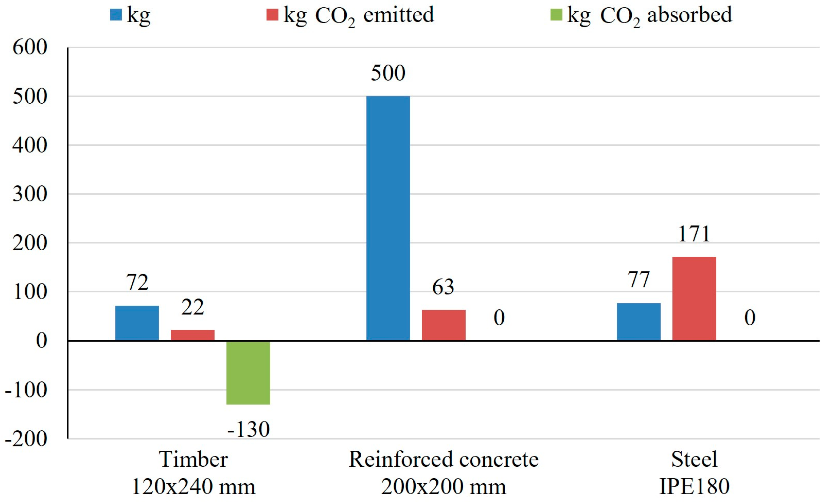
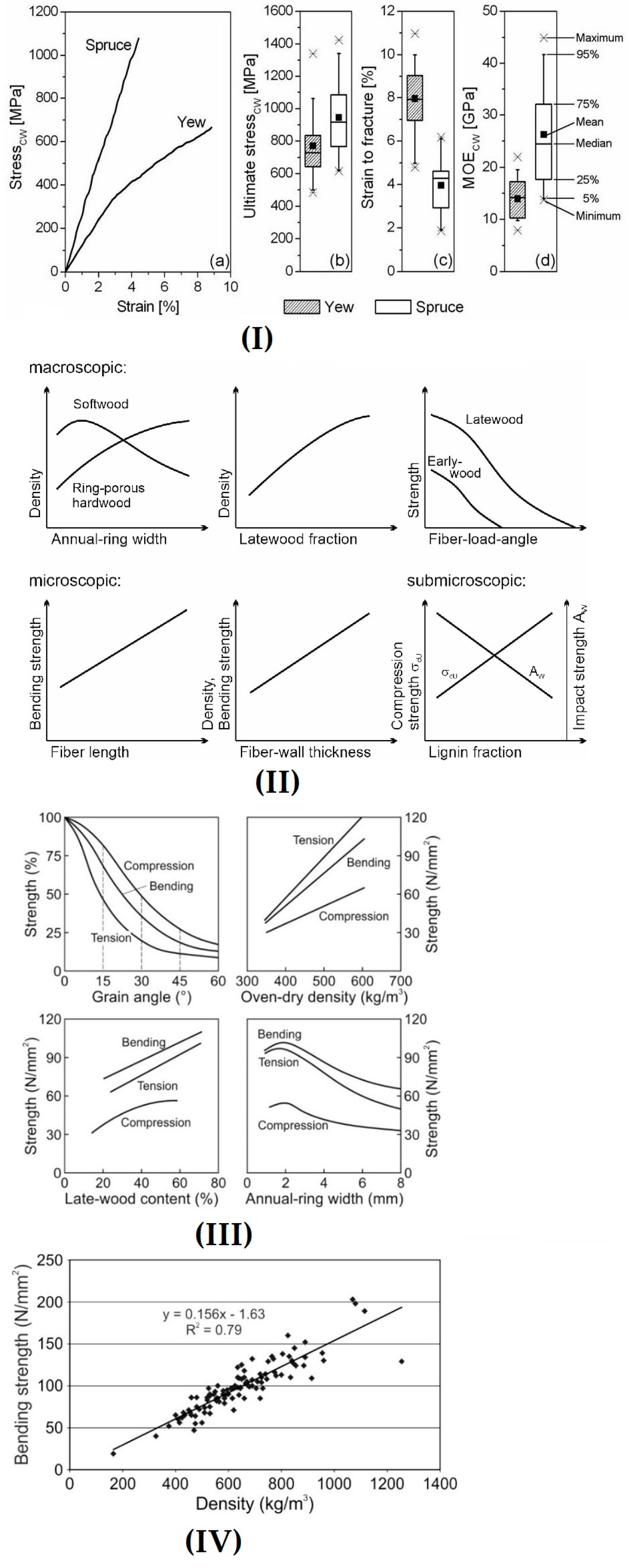
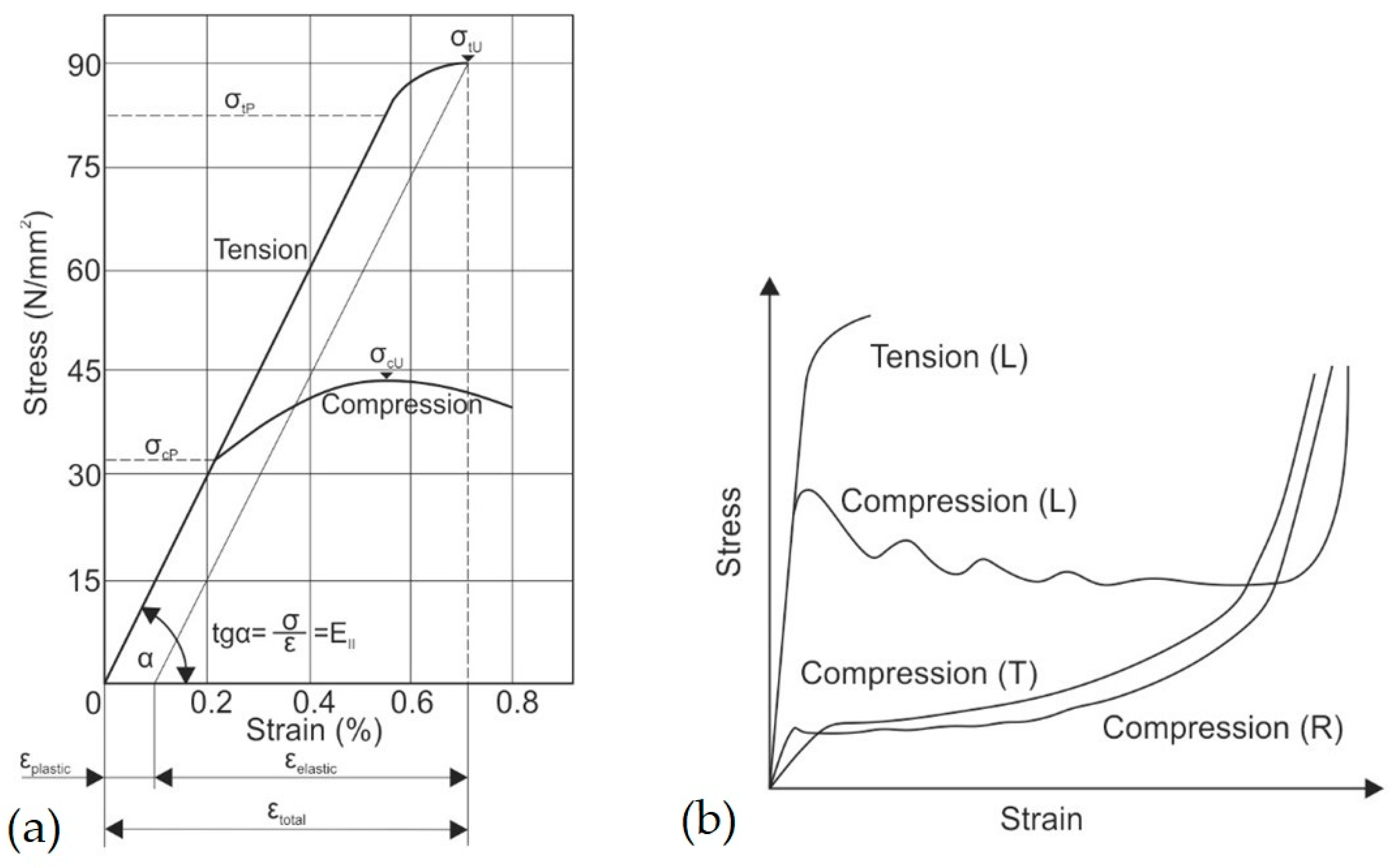
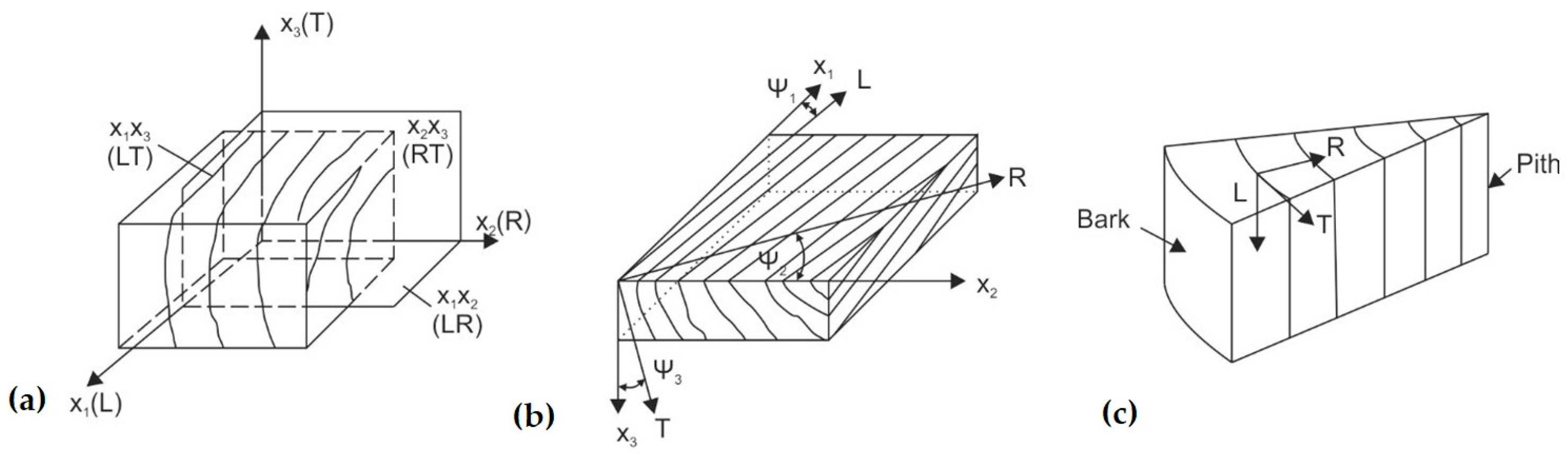
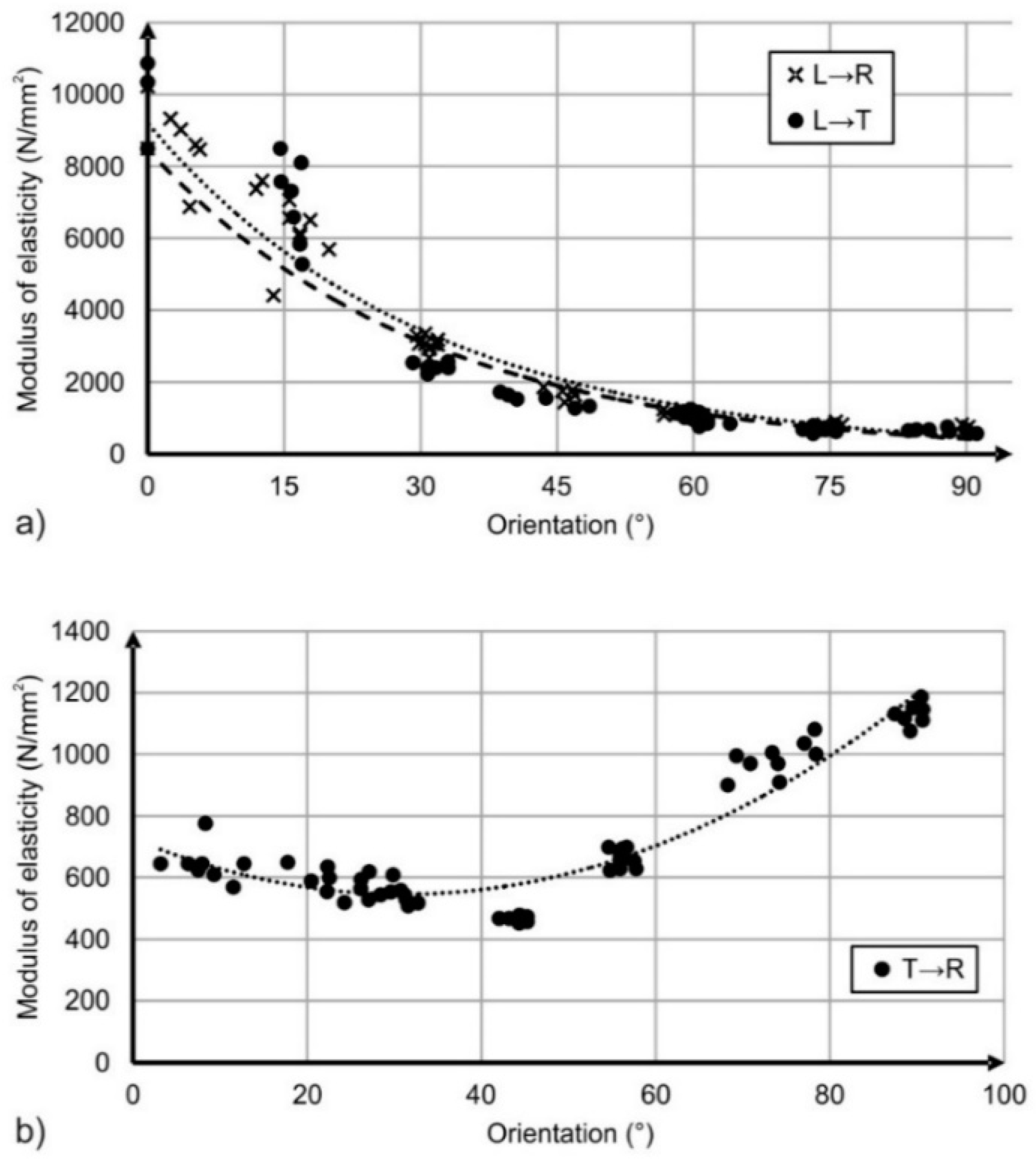
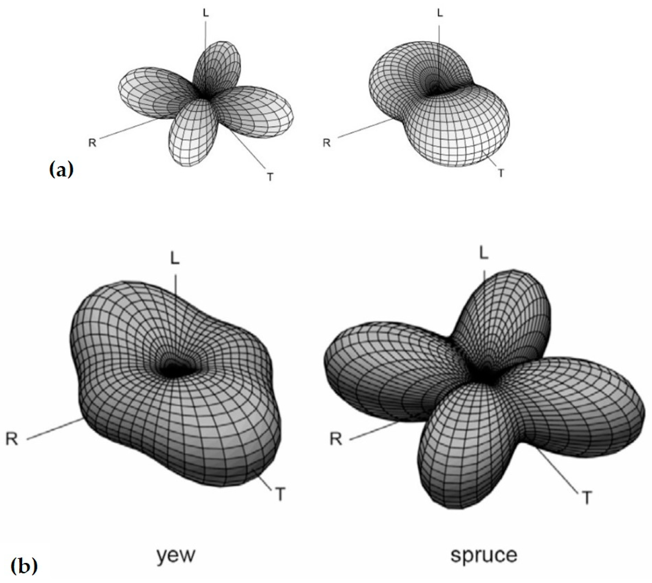
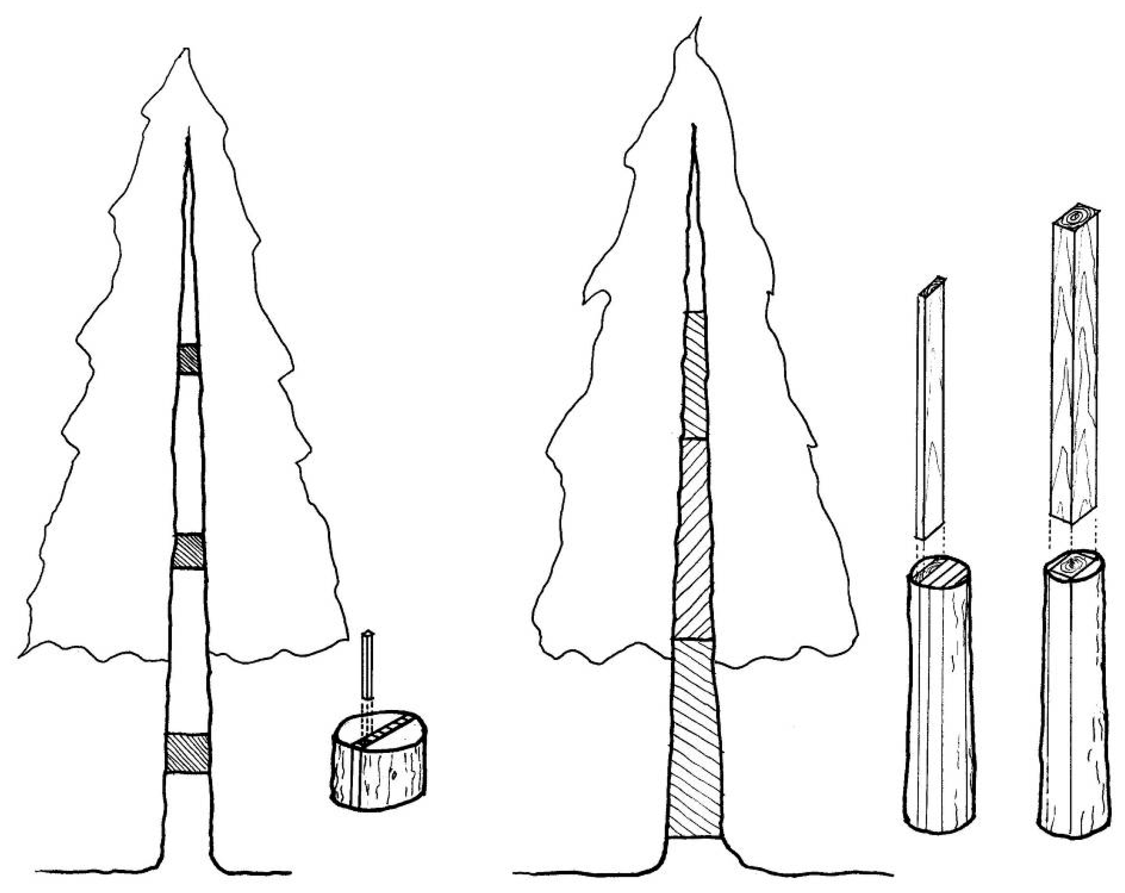
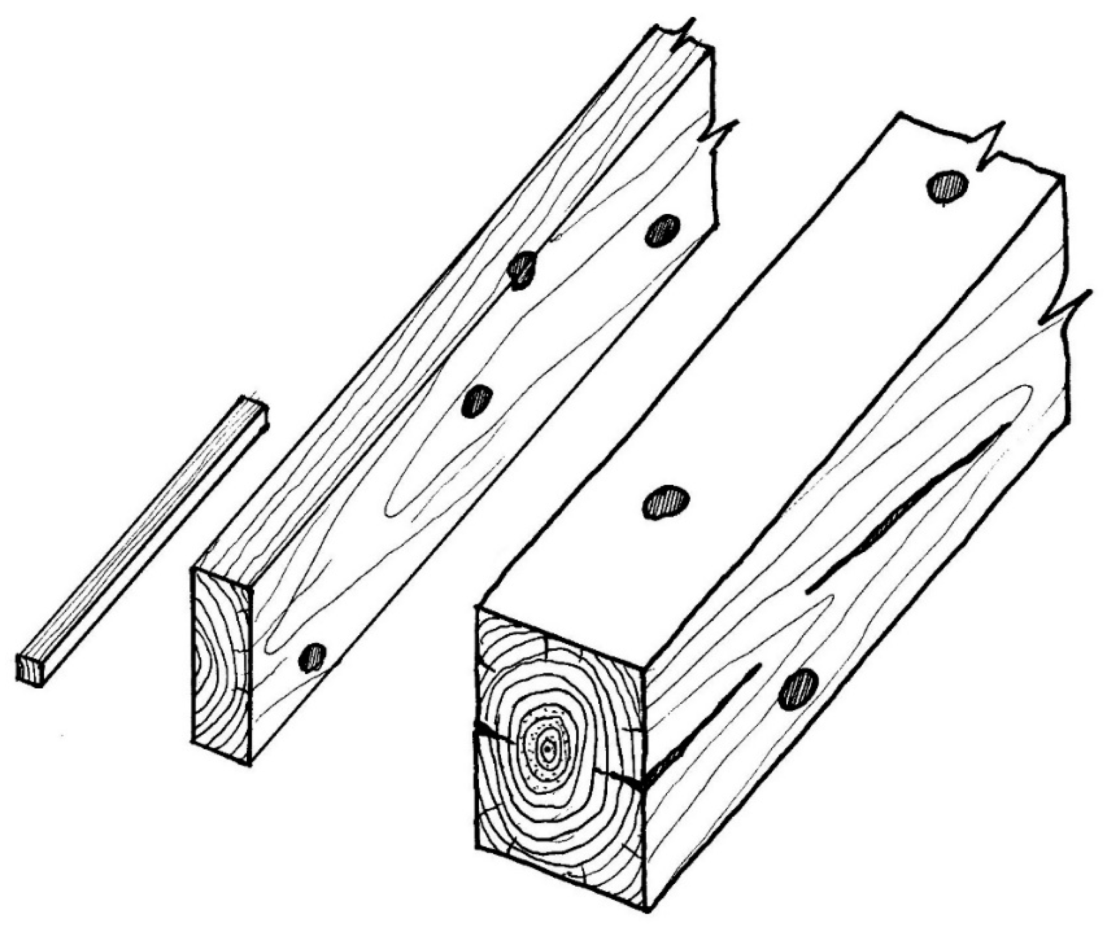
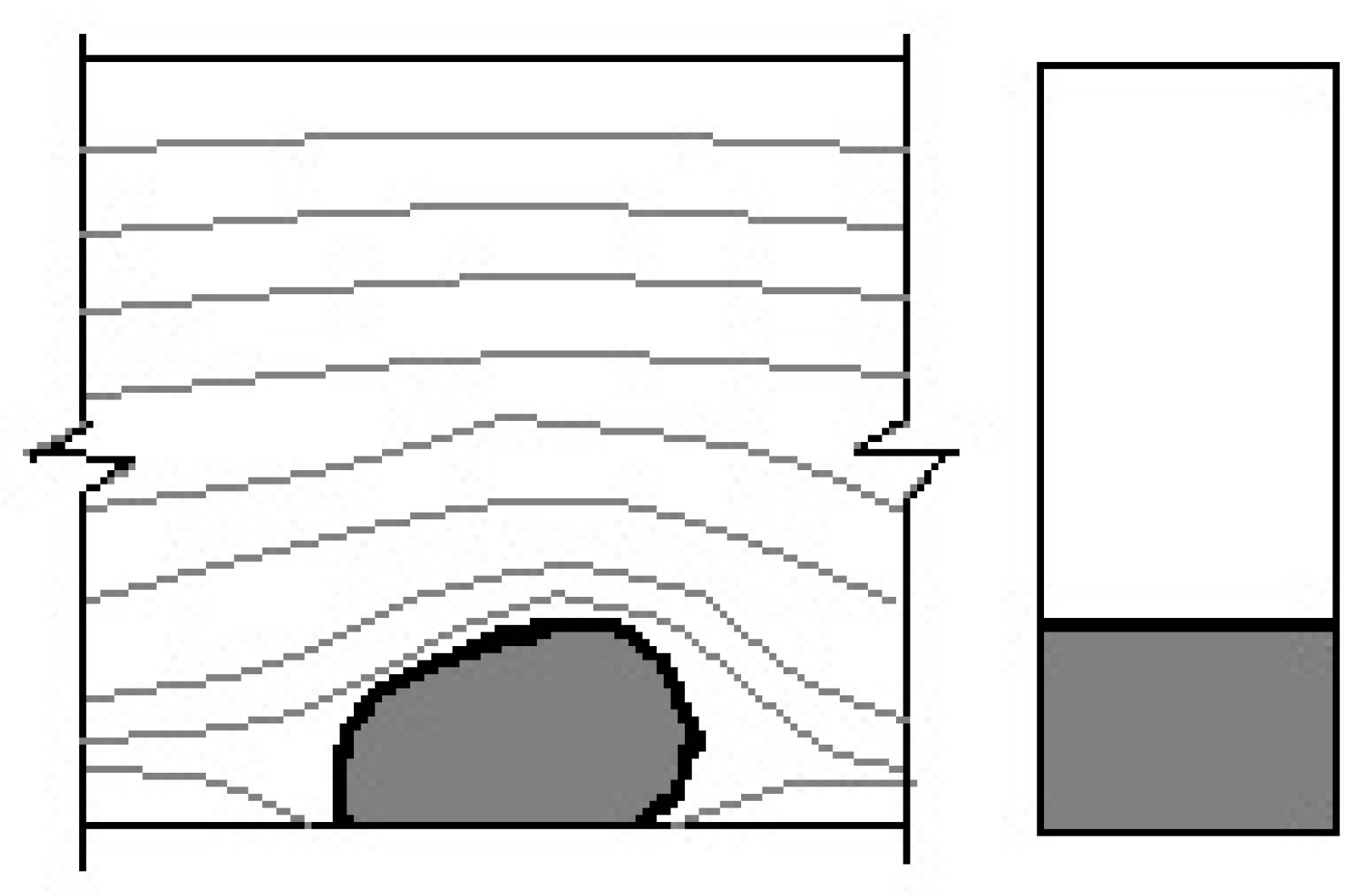
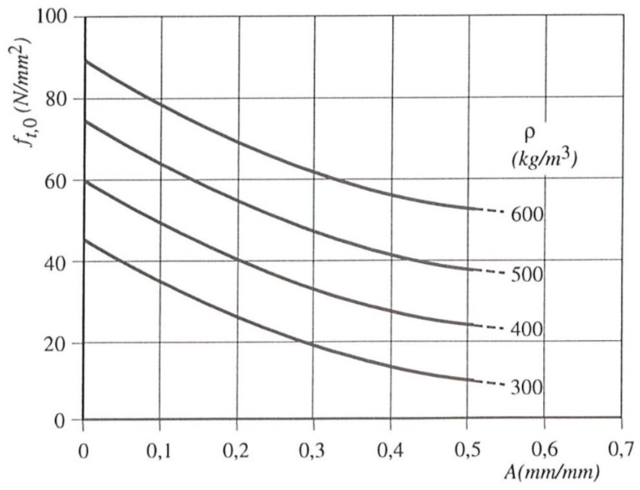
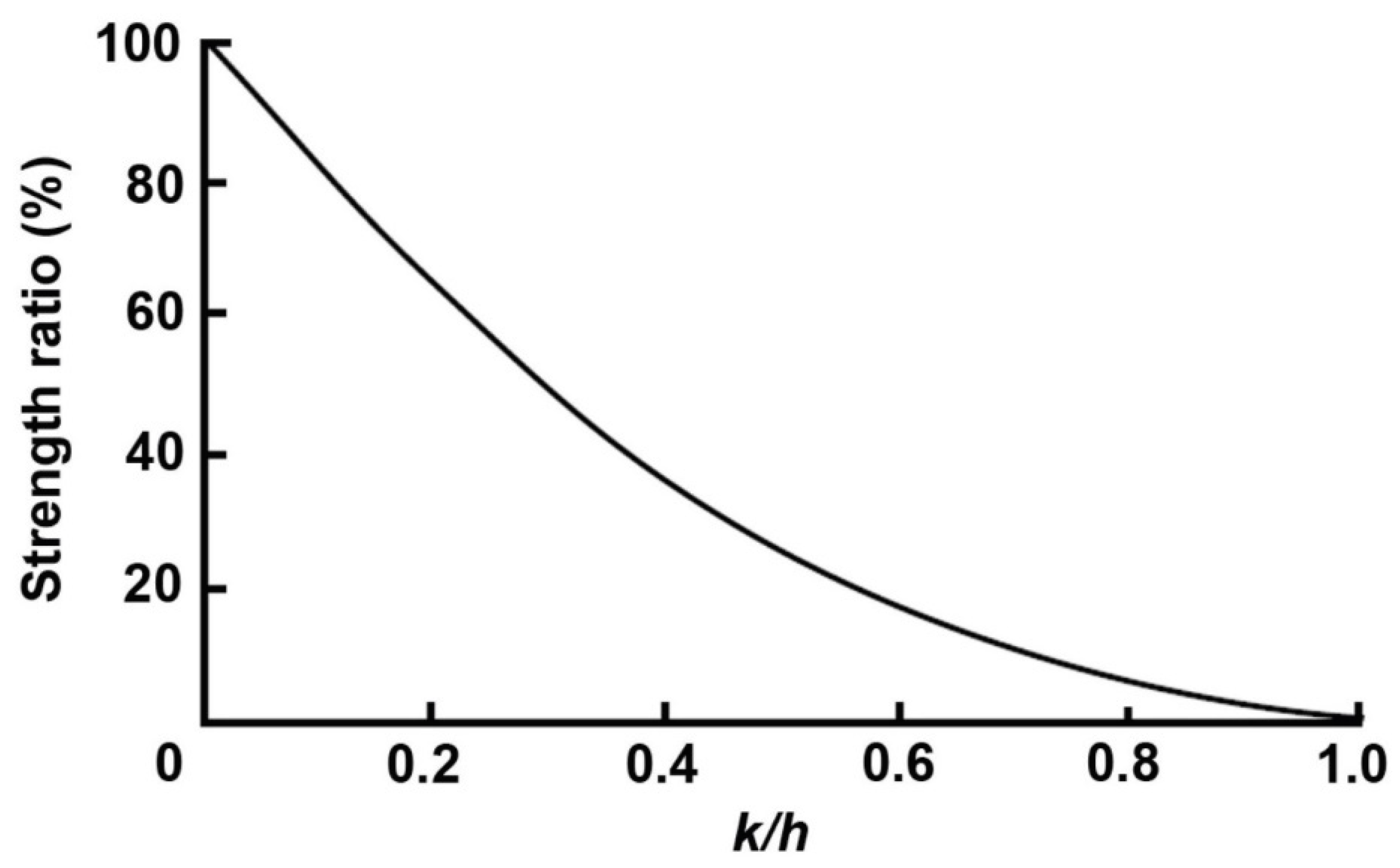
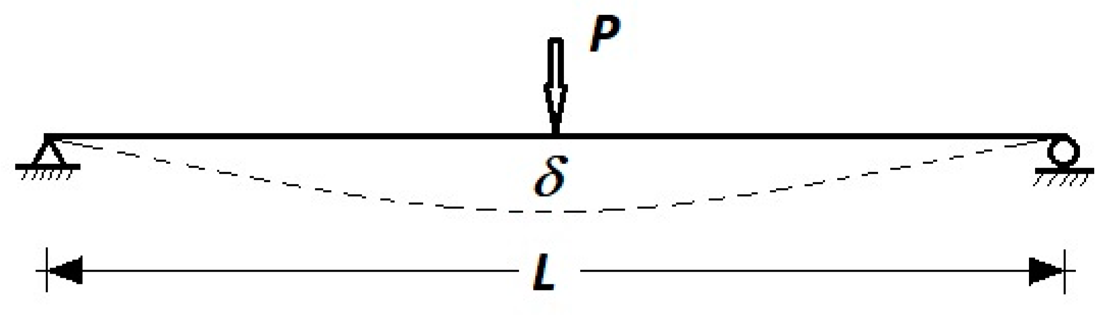
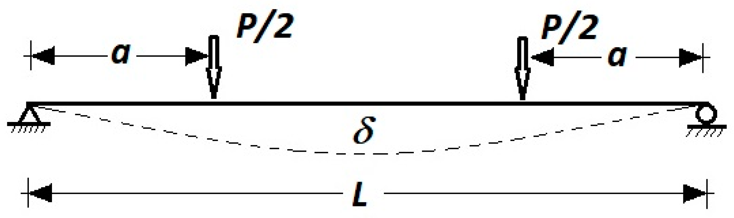
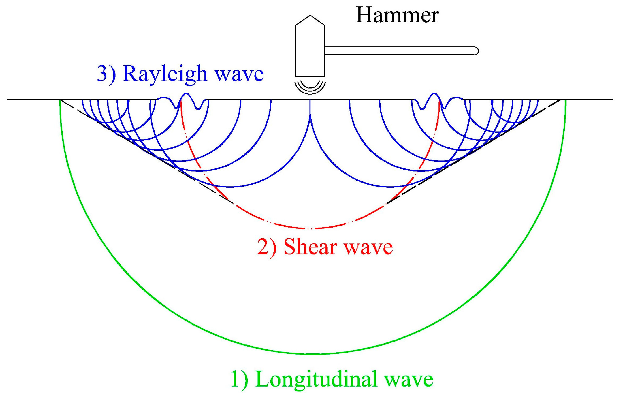
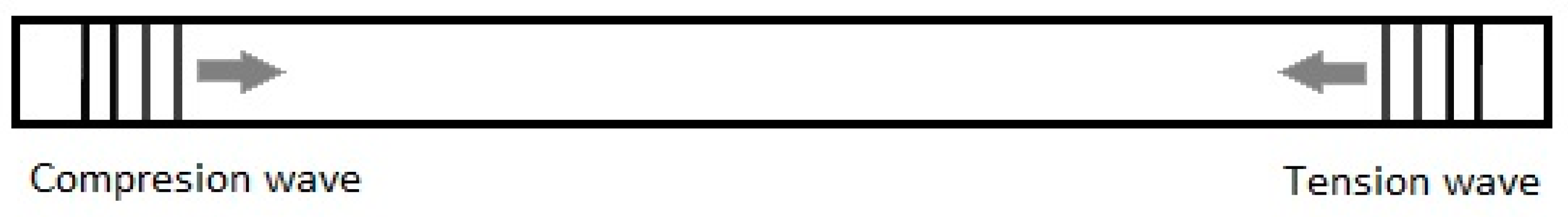
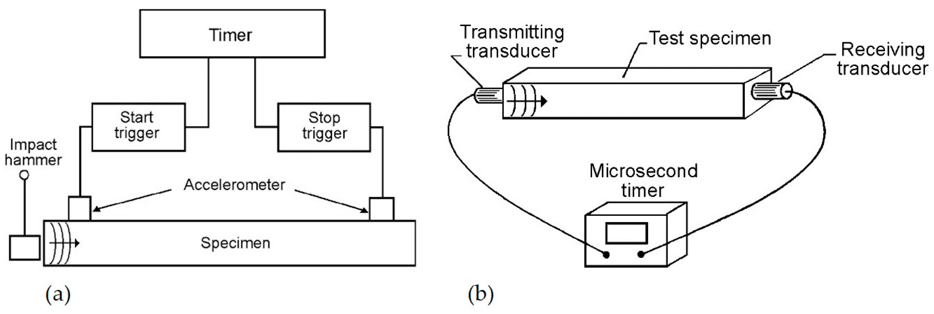
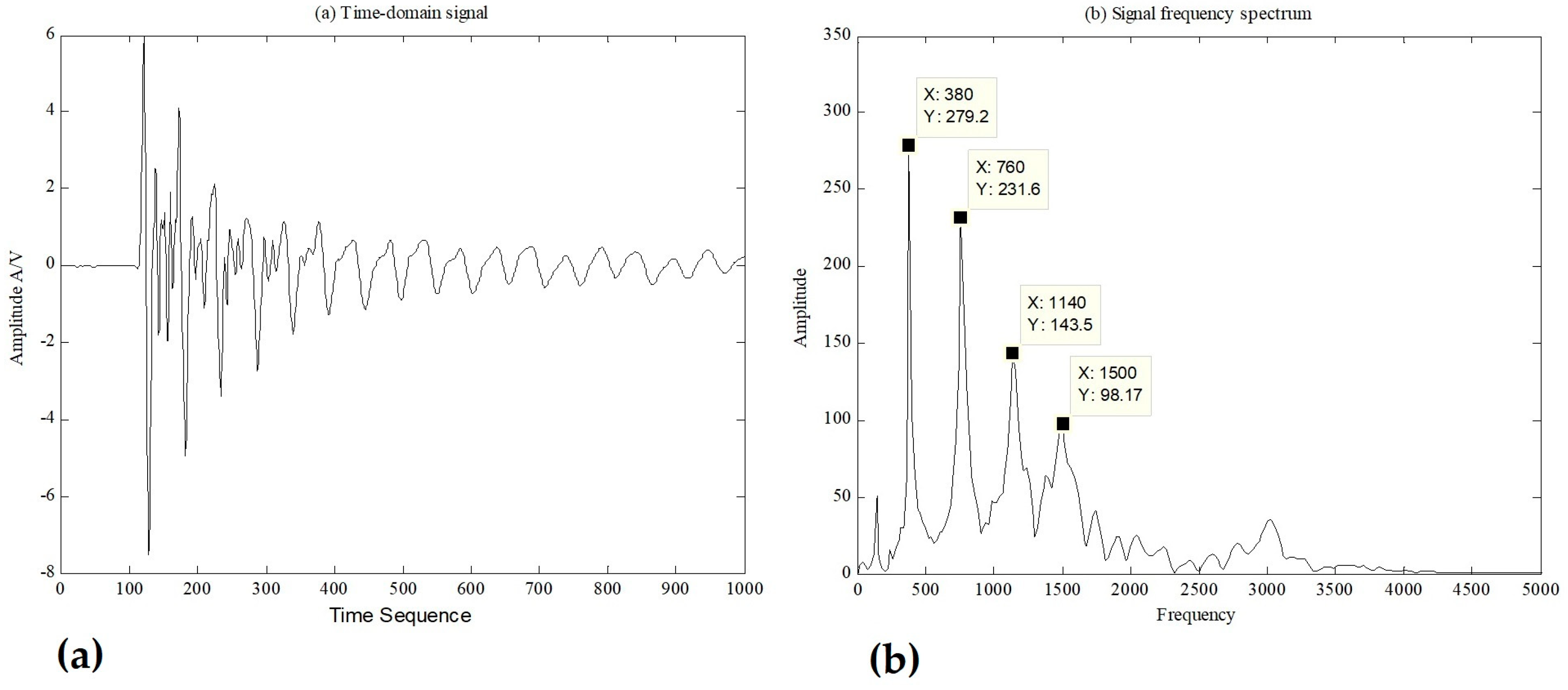
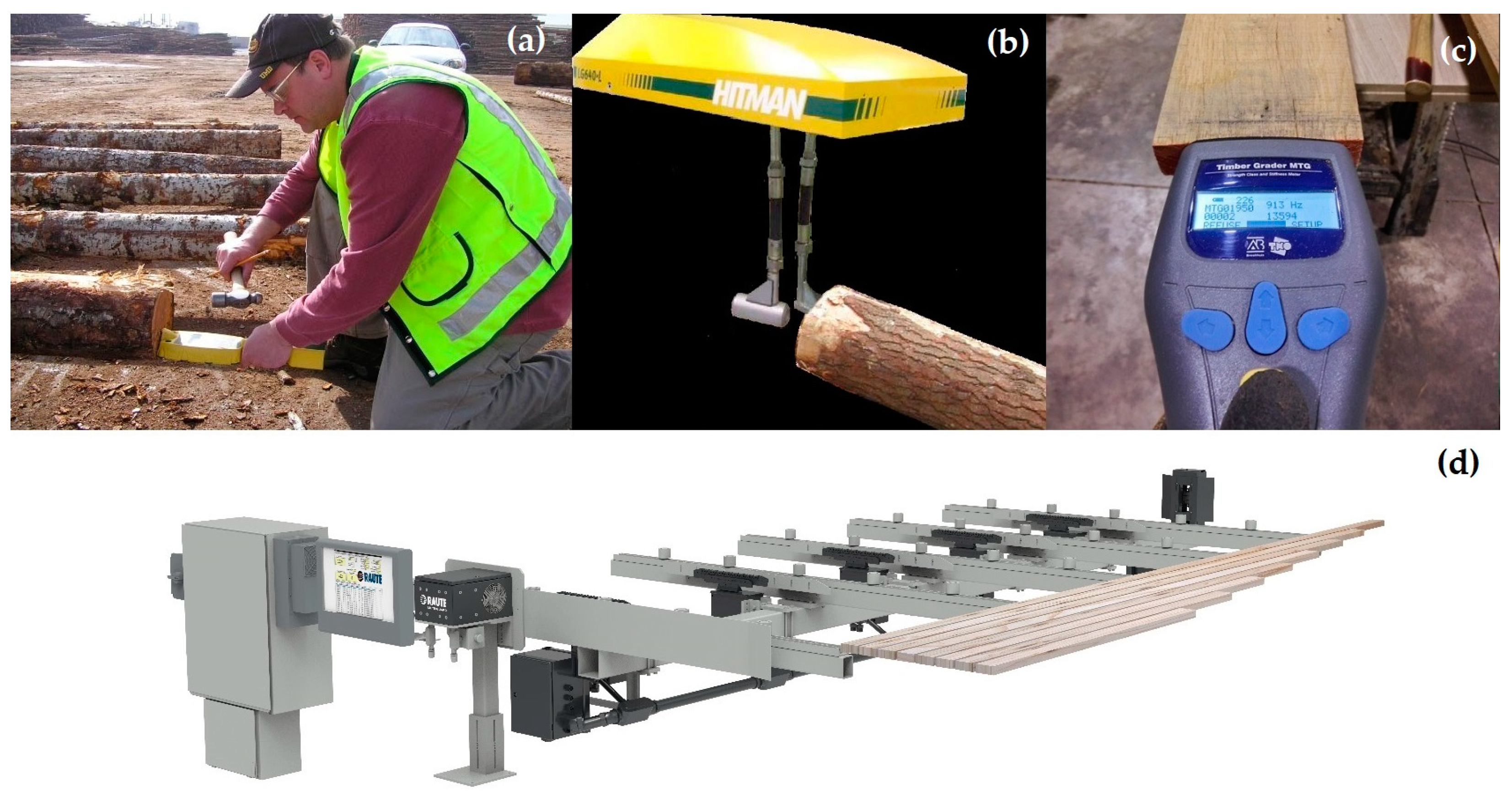
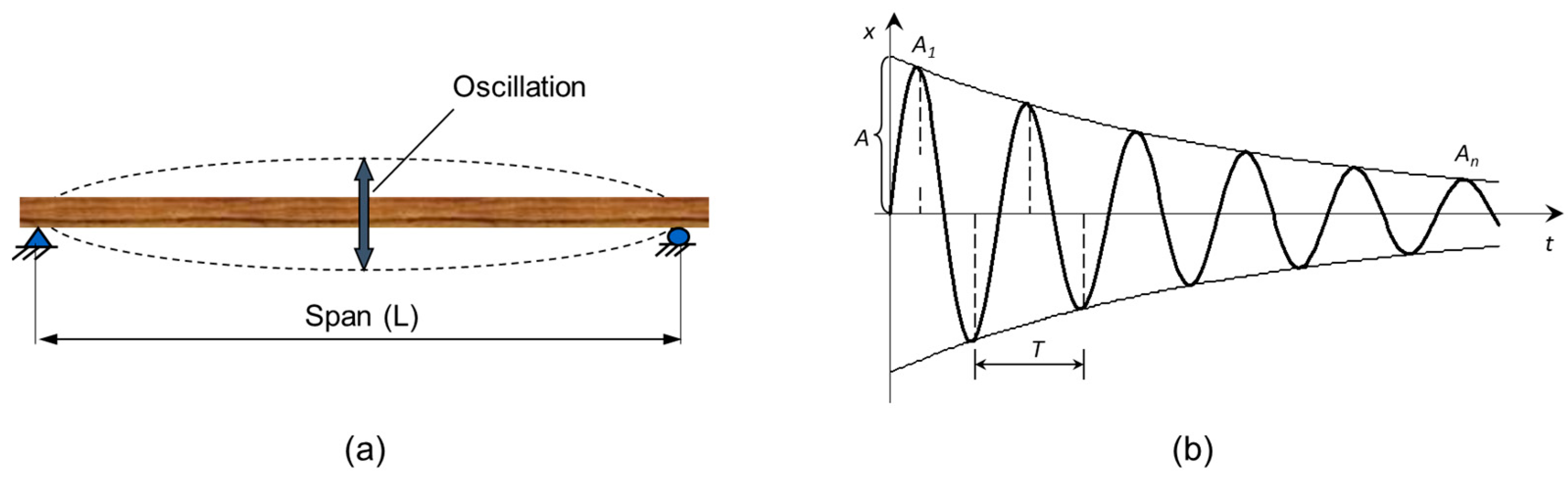
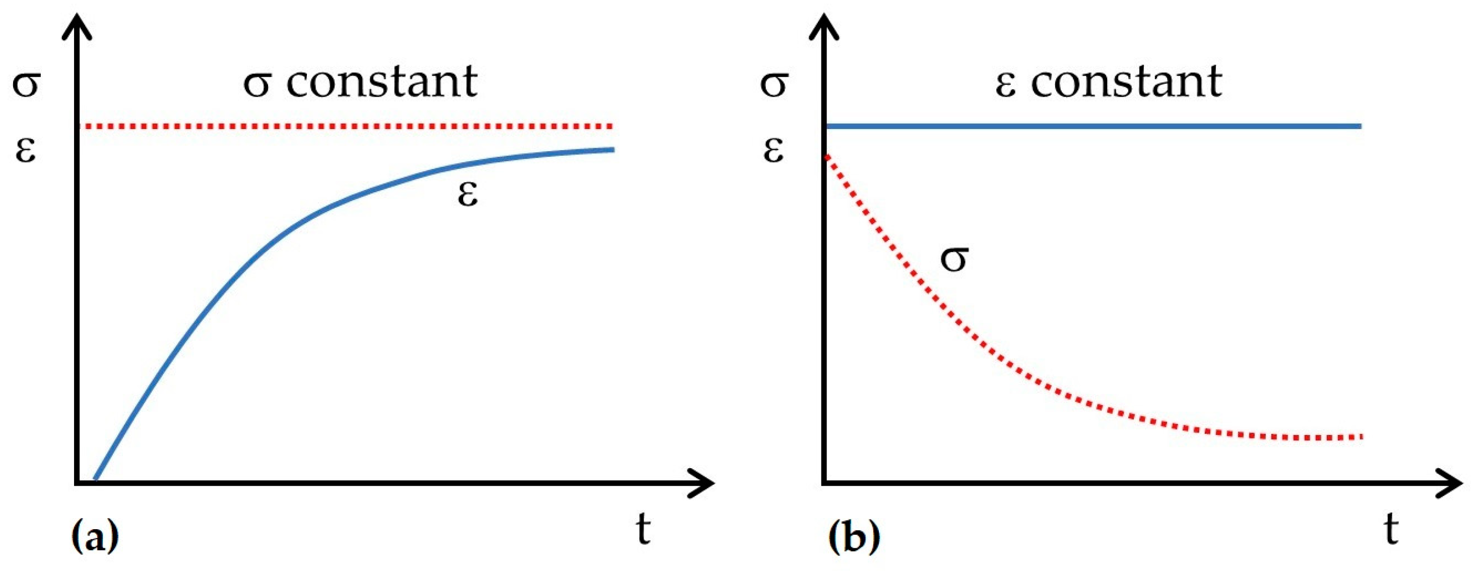
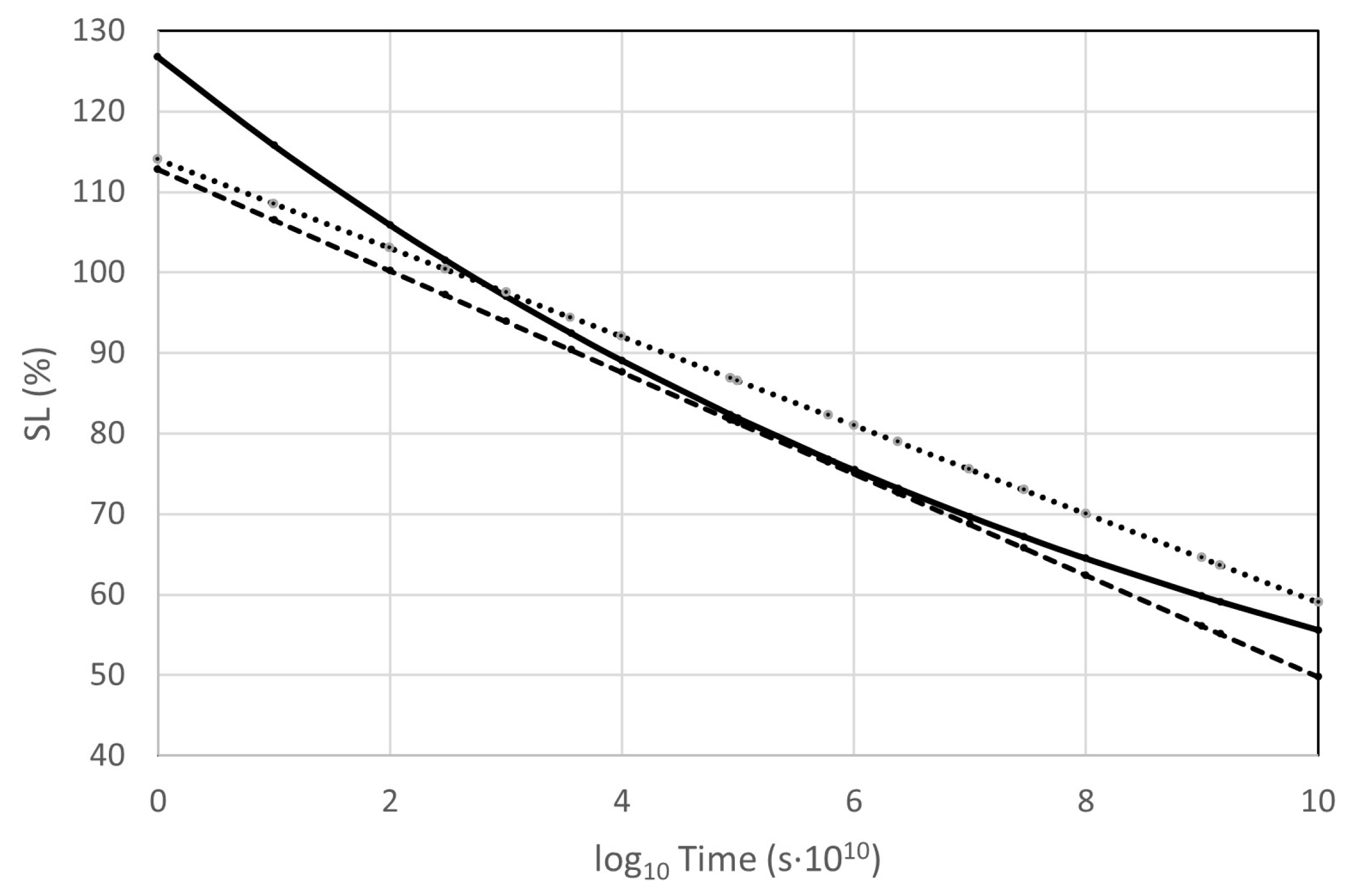
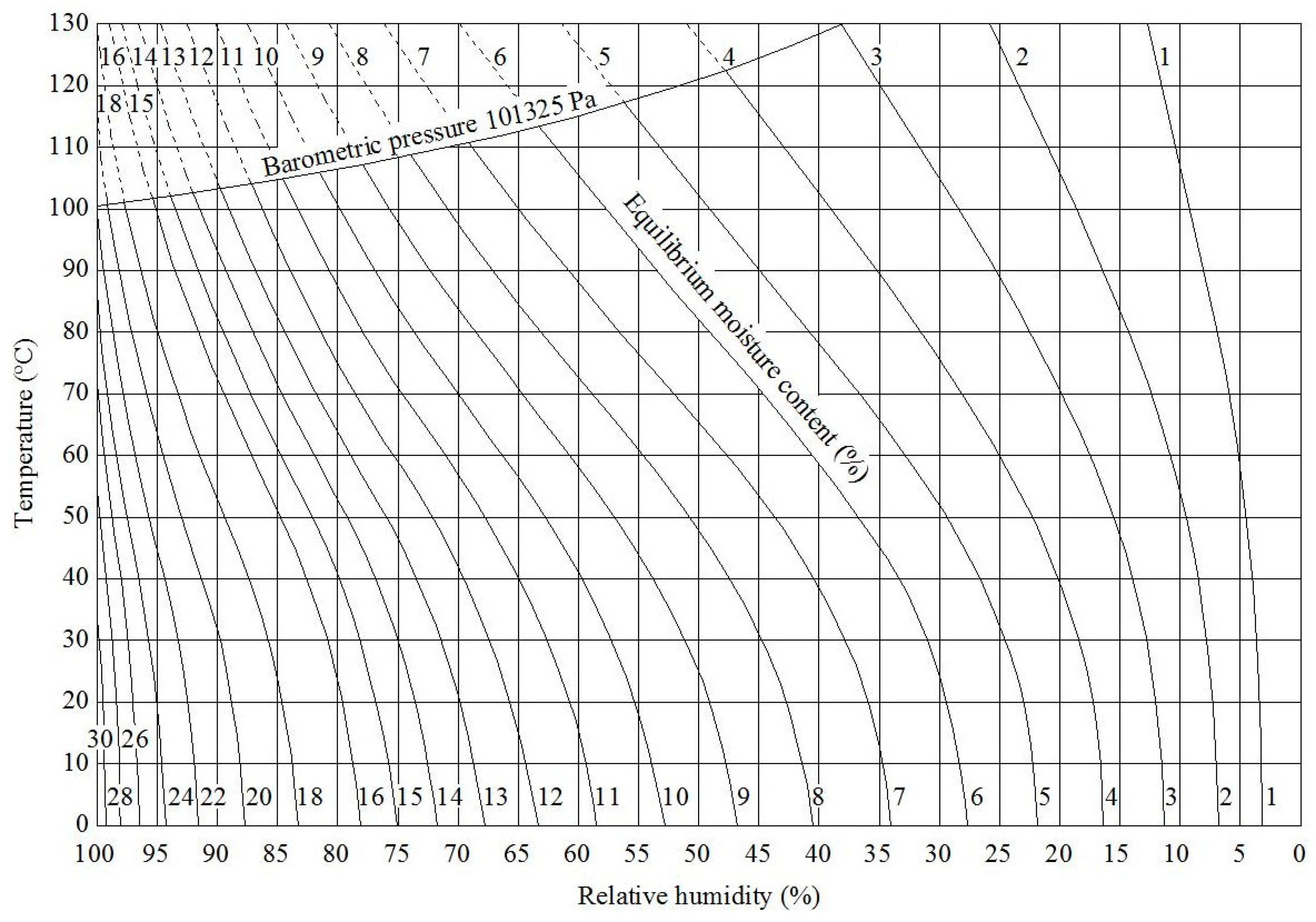
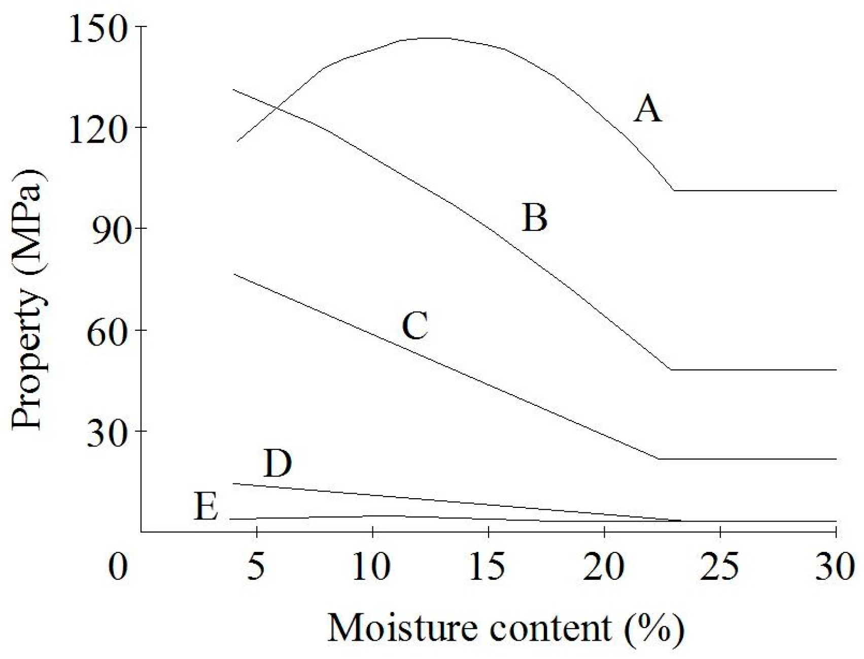
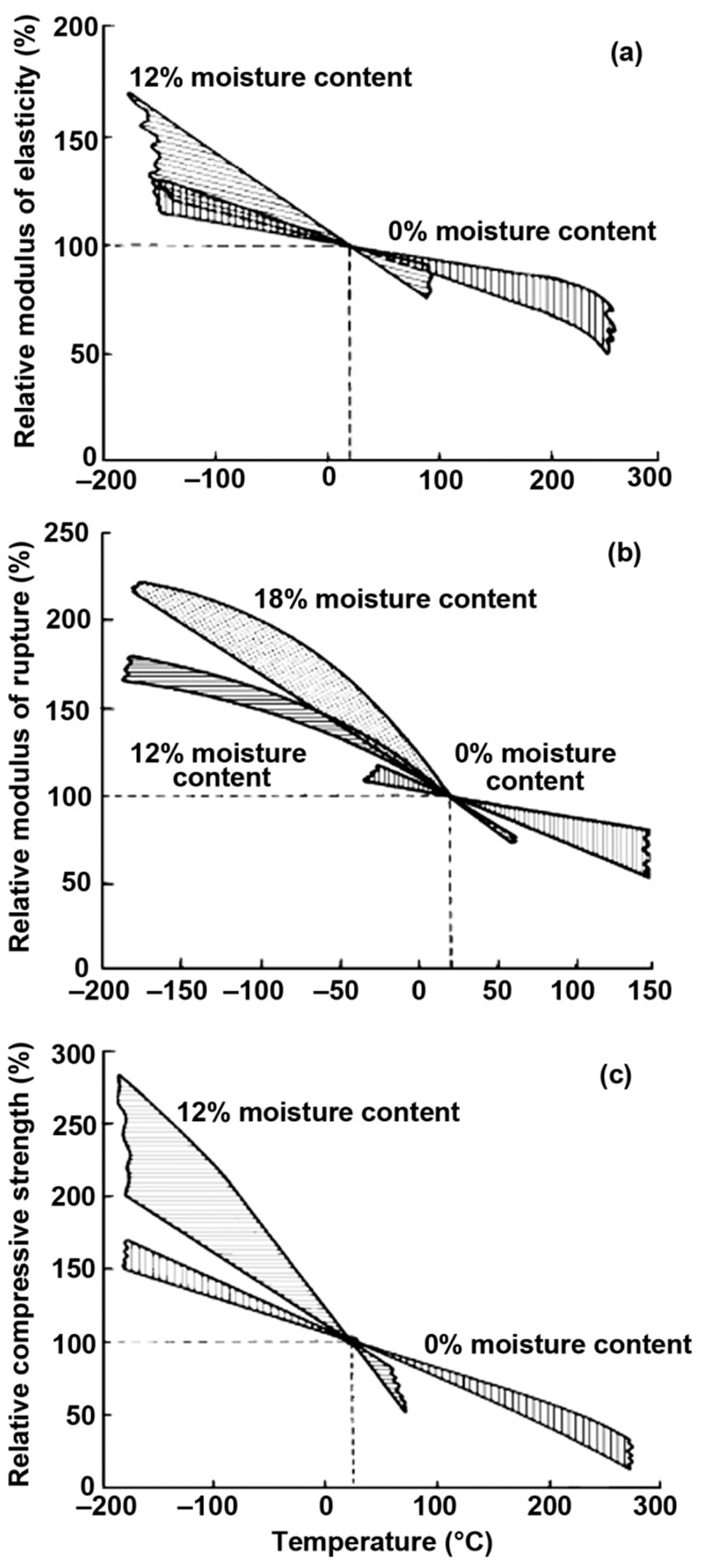
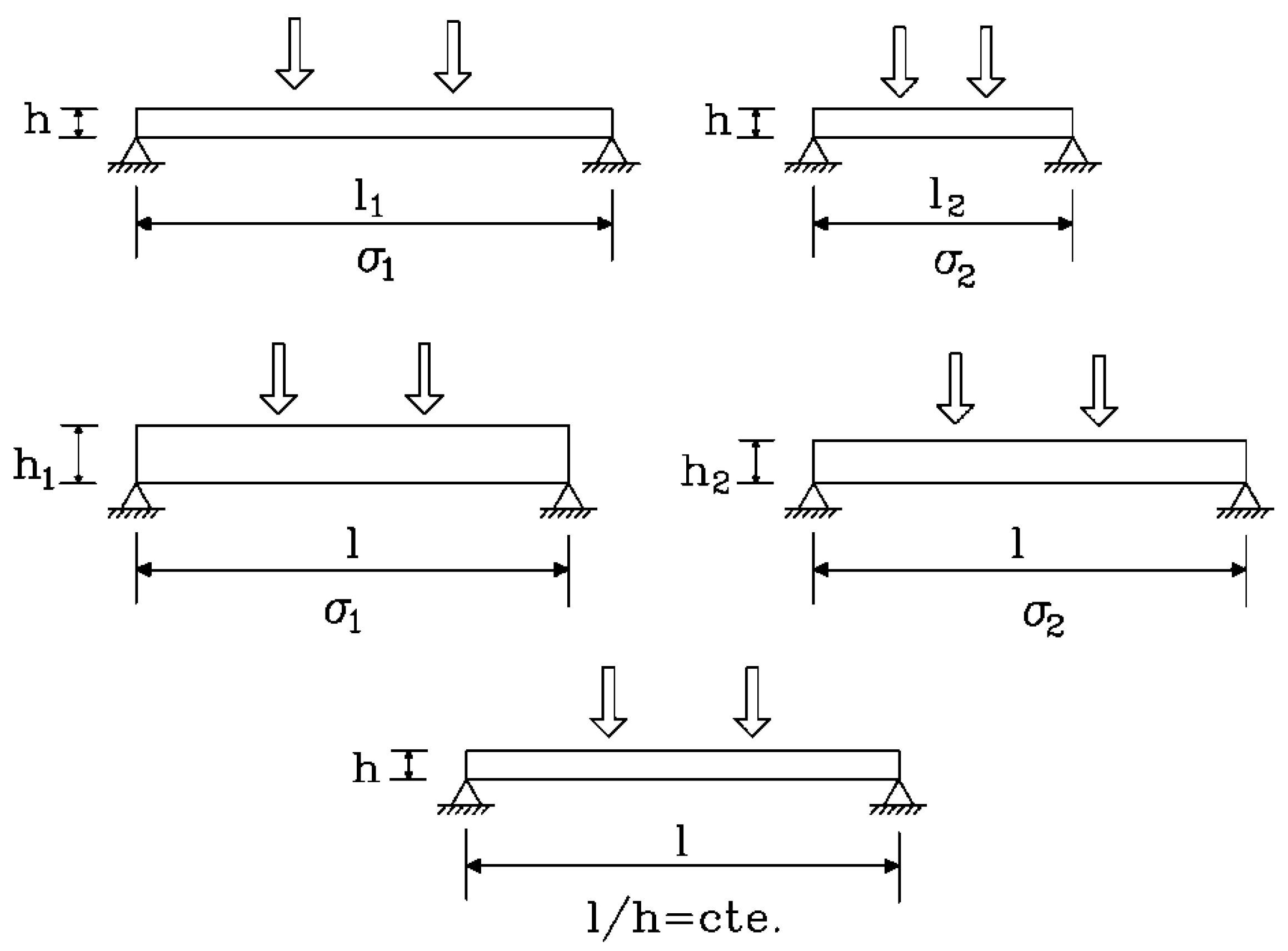
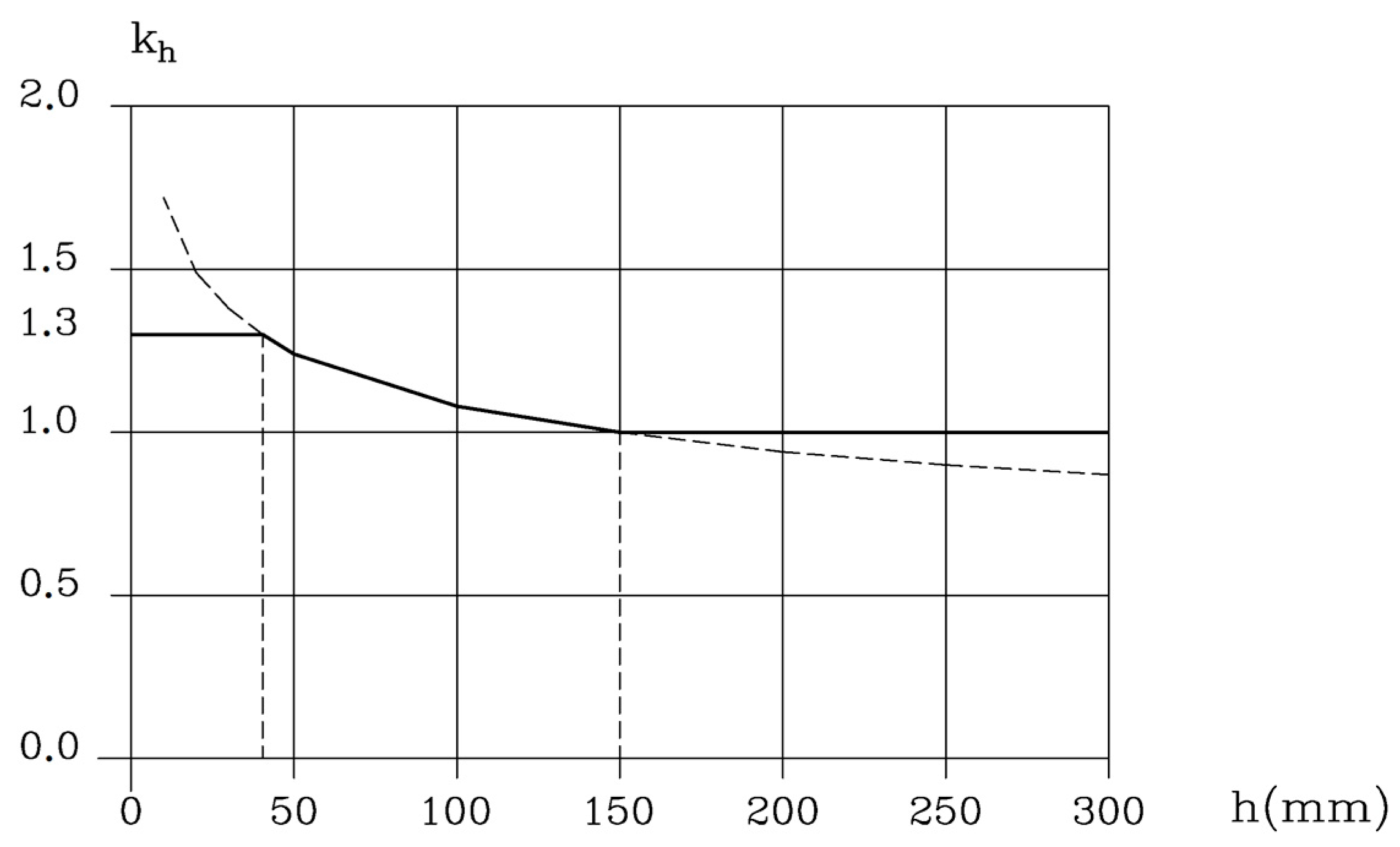
Table A1.
Grading machines approved by the board of review.
| Grading Machine | Agency Support | Machine Manufacturer | Board of Reviews (BOR) Action |
|---|---|---|---|
| 1. Metriguard Model 3300 Transverse Vibration E-Computer Metriguard Model 340 Transverse Vibration E Computer | WCLIB | Metriguard, Inc. P.O. Box 399. Pullman, WA 99163, USA | Granted Model 3300 approval on 12 July 1984 for:
|
| 2. Stress-O-Matic | WWPA | Industrial Woodworking Machines P.O. Box 1465. Garland, TX, USA | Granted approval around 1962. |
| 3. C-L-T (Continuous Lumber Tester) C-L-T Model 7200 HCLT (High Capacity Lumber Tester) | WWPA for C-L-T | Metriguard Inc. P.O. Box 399. Pullman, WA 99163, USA | Granted approval around 1962 for C-L-T. |
| 4. Cook Bolinder Model SG-TF NA | WWPA | Cook Bolinder Ltd. P.O. Box 42. Stansmore, Middlesex, GB HA7,4XD | Granted approval 23 January 1986. |
| 5. X-Ray Lumber Gauge [previously known as Advanced Stress Grader (BOR 10/26/89) no longer available] | SPIB | Newnes Machine Ltd. Company, Sherwood, OR, USA | Granted approval April 1995, subject to:
|
| 6. Dart M. S. R. Testing Machine | CMSA | Eldeco Pty Ltd. Albury, Australia | Granted approval 2 February 1995. |
| 7. Ersson ESG 240-Strength Grader | WCLIB | John Ersson Engineering AB Storvik, Sweden | Granted approval 5 February 1998 |
| 8. Dynagrade Strength Grading Machine | QLMA | Dynalyse AB Partille, Sweden | Granted approval 27 July 2000 |
| 9. Computermatic | WCLIB | Measuring and Process Control Ltd. Essex, UK | Granted approval 8 February 2001 |
| 10. Dimter 403 Grademaster | WCLIB | Dimter GmbH Maschineenfabric Illertissen, Germany | Granted approval 24 April 2003, with the following operational limitations of the machine:
|
| 11. Microtec GoldenEye Lumber Grading Machine | WCLIB | MiCROTEC Srl GmbH Bressanone, Italy | Granted approval 24 April 2003, with the following operation limitations of the machine:
|
| 12. Transverse MSR Grader (TMG) | QFIC | Centre de Recherche Industrielle du Quebec (CRIQ), QC, Canada | Granted approval 29 April 2004, with the following operation limitations of the machine:
|
| 13. Transverse MSR Grader (TMG) 12 | QFIC | Centre de Recherche Industrielle du Quebec (CRIQ), QC, Canada | Granted approval 22 July 2004, with the following operation limitations of the machine:
|
| 14. CRP 360 MSR Testing Machine | QFIC | Conception RP, St-Victor De Deauce, QC, Canada | Granted approval 22 July 2004, with the following operation limitations of the machine:
|
| 15. RE-II (formerly called XLG/LHG+Thumper Strength Grader) | SPIB | Weyerhaeuser | Granted approval 3 February 2005, with the following limitations of the machine:
|
| 16. Transverse MSR Grader (TMG) | QFIC | Centre de Recherche Industrielle du Quebec (CRIQ), QC, Canada | Granted approval 28 July 2005, with the following operation limitations of the machine:
|
| 17. RE-I (formerly called Stand Alone Thumper Strength Grader) | SPIB | Weyerhaeuser | Granted approval 28 July 2005, with the following limitations of the machine:
|
| 18. Falcon Engineering A-Grader | WCLIB | Falcon Engineering, Inglewood, New Zealand | Granted approval 27 July 2006, with the following operation limitations of the machine:
|
| 19. Microtec Goldeneye Model 706 Lumber Grading Machine | WCLIB | MiCROTEC Srl GmbH Bressanone, Italy | Granted approval 2 November 2006, with the following operation limitations of the machine:
|
| 20. Precigrader MSR Grading Machine | CLA | Dynalyse AB, Partille, Sweden | Granted approval 8 February 2007, with operation limitations of the machine as stated in the CLA submission. Modified speed limitation from 180 lugs/min to 260 lugs/min (see SPIB submission 24 January 2019 meeting) |
| 21. LHG:XLG With E-Valuator Stiffness Estimation with Vibration | WWPA | COE Newnes/McGehee | Granted approval 26 April 2007, with the following operation limitations of the machine:
|
| 22. RE-III (formerly called Thumper III) | SPIB | Weyerhaeuser | Granted approval 1 November 2007, with the following operation limitations of the machine:
|
| 23. Ecoustic Board Grader | WCLIB | Calibre Equipment Limited, Wellington, New Zealand | Granted approval 5 January 2012, with the following operation limitations of the machine:
|
| 24. Metriguard 2350 Sonic Grader | WCLIB | Metriguard, Inc. P.O. Box 399 Pullman, WA 99163, USA | Granted approval 18 October 2012, with the following operation limitations of the machine:
|
| 25. MTG | OLMA | Brookhuis Micro Electronics, Enschede, Netherlands | Granted approval 17 April 2014, with the following operation limitations of the machine
|
| 26. MTG BATCH | OLMA | Brookhuis Micro Electronics, Enschede, Netherlands | Granted approval 17 April 2014, with the following operation limitations of the machine
|
| 27. MTG ESCAN | OLMA | Brookhuis Micro Electronics, Enschede, Netherlands | Granted approval 17 April 2014, with the following operation limitations of the machine
|
| 28. VAB—MSR Lug Loader | QFIC | VAB Machines, Inc. Levis, QC, Canada | Granted approval on 26 April 2018, with the following operation limitations of the machine
|
| 29. Microtec Goldeneye Model 806 Lumber Grading Machine | WCLIB | MiCROTEC Srl GmbH Bressanone, Italy | Granted approval 24 January 2019, with the following operation limitations of the machine:
|
| 30. Microtec Goldeneye Model 802 Lumber Grading Machine | WCLIB | MiCROTEC Srl GmbH Bressanone, Italy | Granted approval 24 January 2019, with the following operation limitations of the machine:
|
| 31. USNR Thor Acoustic MSR Grader | PLIB | USNR Woodland, WA, USA | Granted approval 9 January 2020, with the following operation limitations of the machine:
|
References
- Eurostat Website 2018. Available online: https://ec.europa.eu/eurostat/statistics-explained/index.php?title=Wood_products_-_production_and_trade#Primary_wood_products (accessed on 8 February 2023).
- Sostenibilidad: Madera, hormigón o acero. J. Arquit. Madera 2015, 15, 28–33. Available online: https://arquitectura-madera.com/revista-arquitectura-y-madera/ (accessed on 5 June 2023).
- Ramage, M.; Burridge, H.; Busse-Wicher, M.; Fereday, G.; Reynolds, T.; Shah, D.U.; Li Yu, G.W.; Fleming, P.; Densley-Tingley, D.; Alwood, J.; et al. The Wood from the trees: The use of timber in construction. Renew. Sust. Energ. Rev. 2017, 68, 333–359. [Google Scholar] [CrossRef]
- Gordon, J.E. Structures or Why Things Don’t Fall Down; Penguin: London, UK, 1978. [Google Scholar]
- UN General Assembly. Transforming Our World: The 2030 Agenda for Sustainable Development. Resolution Adopted by the General Assembly on 25 September 2015. Available online: https://sdgs.un.org/2030agenda (accessed on 5 June 2023).
- European Commission. Single Market for Green Products Initiative. 2013. Available online: https://ec.europa.eu (accessed on 5 June 2023).
- Fazio, S.; Castelalni, V.; Sala, S.; Schau, E.; Secchi, M.; Zampori, L.; Diaconu, E. Supporting Information to the Characterisation Factors of Recommended EF Life Cycle Impact Assessment Methods; Publications Office of the European Union: Luxembourg, 2018. [Google Scholar]
- Passivhaus Institut. 2019. Available online: https://passivehouse.com (accessed on 5 June 2023).
- Lechón, Y.; de la Rúa, C.; Lechón, J.I. Environmental footprint and life cycle costing of a family house built on CLT structure. Analysis of hotspots and improvement measures. J. Build. Eng. 2021, 39, 102239. [Google Scholar] [CrossRef]
- Esteban, M.; de Miguel, A.; Lechón, J.I. Construcción con madera y sostenibilidad en las ciudades del siglo XXI… y siglos venideros. [Timber construction and sustainability in the 21th century cities and future centuries]. Montes 2018, 131, 53–57. [Google Scholar]
- Stamm, A.J. Wood and Cellulose Science; Ronald Press: New York, NY, USA, 1964. [Google Scholar]
- Fengel, D.; Wegener, G. Wood: Chemistry, Ultrastructure, Reactions; De Gruyter: Berlin, Germany; New York, NY, USA, 1984. [Google Scholar]
- Wagenführ, R. Anatomie des Holzes, 4th ed.; Fachbuchverlag: Leipzig, Germany, 1989. [Google Scholar]
- Butterfield, B. In Proceedings of the IAWA/IUFRO International Workshop of Significance of the Microfibril Angle to Wood Quality. Westport, New Zealand, 21–25 November 1997. [Google Scholar]
- Niemz, P.; Sonderegger, W. Physik des Holzes und der Holzwerkstoffe, 2nd ed.; Carl Hanser Verlag: München, Germany, 2021. [Google Scholar]
- Toumpanaki, E.; Shah, D.R.U.; Eichhorn, S.J. Beyond what meets the eye: Imaging and imagining wood mechanical-structural properties. Adv. Mater. 2021, 33, 2001613. [Google Scholar] [CrossRef]
- Keunecke, D. Elasto-Mechanical Characterisation of Yew and Spruce Wood with Regard to Structure-Property Relationships. Ph.D. Dissertation, ETH Zürich, Zürich, Switzerland, 2008; 159p. [Google Scholar] [CrossRef]
- Eder, M.; Rüggeberg, M.; Burgert, I. A close-up view of the mechanical design of arborescent plants at different levels of hierarchy—Requirements and structural solutions. N. Z. J. For. Sci. 2009, 39, 115–124. [Google Scholar]
- Stanzl-Tschegg, S.; Keunecke, D.; Tschegg, E. Fracture tolerance of reaction wood (yew and spruce wood in TR crack propagation system). J. Mech. Behav. Biomed. 2011, 4, 688–698. [Google Scholar] [CrossRef] [PubMed]
- Niemz, P.; Teischinger, A.; Sandberg, D. Springer Handbook of Wood Science and Technology; Springer: Heidelberg, Germany, 2023; in press. [Google Scholar]
- Sell, J. Eigenschaften und Kenngrössen von Holzarten, 4th ed.; Dietikon; Baufachverlag: Zürich, Switzerland, 1997. [Google Scholar]
- Ozyhar, T. Moisture and Time Dependent Orthotropic Mechanical Characterization of Beech Wood. Ph.D. Dissertation, ETH Zürich, Zürich, Switzerland, 2013. [Google Scholar] [CrossRef]
- Voigt, W. Lehrbuch der Kristallphysik; B.G. Teubner: Leipzig, Germany, 1928. [Google Scholar]
- Höring, G. Zur Elastizität des Fichtenholzes. Z. Für Tech. Phys. 1933, 12, 369–379. [Google Scholar]
- Keylwerth, R. Die Anisotrope Elastizität des Holzes und der Lagenhölzer; VDI Verlag: Düsseldorf, Germany, 1951. [Google Scholar]
- Kollmann, F.F.P. Technologie des Holzes und der Holzwerkstoffe, 2nd ed.; Springer: Berlin/Göttingen/Heidelberg, Germany, 1951. [Google Scholar]
- Bodig, J.; Jayne, B.A. Mechanics of Wood and Wood Composites, 1st ed.; Van Nostrand Reinhold: New York, NY, USA, 1982. [Google Scholar]
- Altenbach, H.; Altenbach, J.; Rikards, R. Einführung in die Mechanik der Laminat-und Sandwichtragwerke; Deutscher Verlag für Grundstoffindustrie: Stuttgart, Germany, 1996. [Google Scholar]
- Von Halász, R.; Scheer, C. Holzbau-Taschenbuch. Band 1: Grundlagen, Entwurf und Konstruktionen, 8th ed.; Ernst & Sohn: Berlin, Germany, 1986. [Google Scholar]
- Hankinson, R.L. Investigation of Crushing Strength of Spruce at Varying Angles of Grain; Air Force Information Circular No. 259; U.S. Air Service: Washington, DC, USA, 1921. [Google Scholar]
- Burgert, I. Die Mechanische Bedeutung der Holzstrahlen im Lebenden Baum. Ph.D. Thesis, Universität Hamburg, Hamburg, Germany, 2000. [Google Scholar]
- Sjölund, J. Effect of Cell Structure Geometric and Elastic Parameters on Wood Rigidity. Ph.D. Thesis, Universität Aalto, Espoo, Finland, 2015. [Google Scholar]
- Grimsel, M. Mechanisches Verhalten von Holz: Struktur- und Parameteridentifikation eines Anisotropen Werkstoffes. Ph.D. Thesis, TU Dresden, Dresden, Germany, 1999. [Google Scholar]
- Clauß, S.; Pescatore, C.; Niemz, P. Anisotropic elastic properties of common ash (Fraxinus excelsior L.). Holzforschung 2014, 68, 941–949. [Google Scholar] [CrossRef] [Green Version]
- Timoshenko, G. History of Strength of Materials; MxGraw-Hill Book Company, Inc.: New York, NY, USA; The Maple Press Company: York, PA, USA, 1953. [Google Scholar]
- Vitruvius. The Ten Books on Architecture; Morgan, M.H., Translator; Harvard University Press: Cambridge, MA, USA, 1914. [Google Scholar]
- Arriaga, F. Los Diez Libros de Arquitectura de Vitruvio y la Carpintería. Texto y Comentarios de lo Tratado en el Capítulo IX “De la Madera” del Libro Segundo (The Ten Books on Architecture of Vitruvius and the Carpentry. Text and Comments on Chapter IX “Timber” of the Second Book); AITIM: Madrid, Spain, 1996; No. 180; pp. 53–60. [Google Scholar]
- Galileo. Two New Sciences; Crew, H., de Salvio, A., Translators; The Macmillan Company: New York, NY, USA, 1933. [Google Scholar]
- Hooke, R. De Potentia Restitutiva; Royal Society: London, UK, 1678. [Google Scholar]
- Belidor, B.F. La Science des Ingeniénieurs; Source Gallica.bnf.fr/Bibliothèque Nationale de France; C. Jombert: Paris, France, 1729. [Google Scholar]
- Booth, L.G. The Strength Testing of Timber during the 17th and 18th Centuries. J. Inst. Wood Sci. 1964, 3, 5–30. [Google Scholar]
- Guilhiermoz, P. De L’équivalence des Anciennes Mesures; A Proposal d’une Publication Recénte; Bibliotheque de l’École des Chartes: Paris, France, 1913. [Google Scholar]
- ISO 13061-3:2014; Physical and Mechanical Properties of Wood. Test Methods for Small Clear Specimens. Part 3: Determination of Ultimate Strength in Static Bending. International Organization for Standardization: Geneva, Switzerland, 2014.
- ISO 13061-4:2014; Physical and Mechanical Properties of Wood. Test Methods for Small Clear Specimens. Part 4: Determination of Modulus of Elasticity in Static Bending. International Organization for Standardization: Geneva, Switzerland, 2014.
- ISO 13061-6:2014; Physical and Mechanical Properties of Wood. Test Methods for Small Clear Wood Specimens. Part 6: Determination of Ultimate Tensile Stress Parallel to Grain. International Organization for Standardization: Geneva, Switzerland, 2014.
- ISO 13061-17:2017; Physical and Mechanical Properties of Wood. Test Methods for Small Clear Wood Specimens. Part 17: Determination of Ultimate Stress in Compression Parallel to Grain. International Organization for Standardization: Geneva, Switzerland, 2017.
- ISO 13061-8:2022; Physical and Mechanical Properties of Wood. Test Methods for Small Clear Wood Specimens. Part 8: Determination of Ultimate Strength in Shearing Parallel to Grain. International Organization for Standardization: Geneva, Switzerland, 2022.
- ISO 13061-2:2014; Physical and Mechanical Properties of Wood. Test Methods for Small Clear Wood Specimens. Part 2: Determination of Density for Physical and Mechanical Tests. International Organization for Standardization: Geneva, Switzerland, 2014.
- ASTM D143:2021; Standard Test Methods for Small Clear Specimens of Timber. American Society for Testing and Materials: Philadelphia, PA, USA, 2021.
- Madsen, B.; Nielsen, L.F. Structural Behaviour of Timber; Timber Engineering Ltd.: North Vancouver, BC, Canada, 1992; 405p. [Google Scholar]
- ISO 8375:1985; Solid Timber in Structural Sizes. Determination of Some Physical and Mechanical Properties. International Organization for Standardization: Geneva, Switzerland, 1985.
- ISO 8375:2017; Timber Structures. Glued Laminated Timber. Test Methods for Determination of Physical and Mechanical Properties. International Organization for Standardization: Geneva, Switzerland, 2017.
- EN 408:2010+A1:2012; Timber Structures. Structural Timber and Glued Laminated Timber. Determination of Some Physical and Mechanical Properties. European Committee of Standardization (CEN): Brussels, Belgium, 2012.
- EN 384:2016+A2:2022; Structural Timber. Determination of Characteristic Values of Mechanical Properties and Density. European Committee of Standardization (CEN): Brussels, Belgium, 2022.
- ASTM D198-21:2021; Standard Test Methods of Static Tests for Lumber in Structural Sizes. American Society for Testing and Materials: Philadelphia, PA, USA, 2021.
- ISO 13910:2014; Timber Structures. Strength Graded Timber. Test Methods for Structural Properties. International Organization for Standardization: Geneva, Switzerland, 2014.
- Ridley-Ellis, D.; Stapel, P.; Baño, V. Strength grading of sawn timber in Europe: An explanation for engineers and researchers. Eur. J. Wood Prod. 2016, 74, 291–306. [Google Scholar] [CrossRef]
- EN 14081-1:2016+A1:2019; Timber Structures—Strength Graded Structural Timber with Rectangular Cross Section—Part 1: General Requirements. Committee of Standardization (CEN): Brussels, Belgium, 2019.
- EN 14081-2:2018; Timber Structures—Strength Graded Structural Timber with Rectangular CROSS section—Part 2: Machine Grading; Additional Requirements for Initial Type Testing. European Committee of Standardization (CEN): Brussels, Belgium, 2018.
- Ross, R.J. Wood Handbook: Wood as an Engineering Material; U.S. Dept. of Agriculture, Forest Service, Forest Products Laboratory: Madison, WI, USA, 2021; 509p. [Google Scholar]
- Wolfe, R. Research challenges for structural use of small-diameter round timbers. Forest Prod. J. 2000, 50, 21–29. [Google Scholar]
- Glos, P. Strength Grading. Basis of Design, Material Properties, Structural Components and Joints; Timber Engineering STEP 1; Centrum Hout: Almere, The Netherlands, 1995; pp. A6/1–A6/8. [Google Scholar]
- Glos, P. Technical and economical possibilities of timber strength grading in small and medium sized companies. In SAH Bulletin 1983/1’; Schweizerische Arbeitsgemeinschaft fur Holzforschung: Zurich, Switzerland, 1983. [Google Scholar]
- Center for Wood Science and Technology. Rate of Growth. 2016. Available online: https://blogs.napier.ac.uk/cwst/speed-of-growth/ (accessed on 26 October 2022).
- Johansson, C.J.; Boström, L.; Bräuner, L.; Hoffmeyer, P.; Holmqvist, C.; Solli, K.H. Laminations for Glued Laminated Timber. Establishment of Strength Classess for Visual Strength Grades and Machine Settings for Glulam Laminations of Nordic Origin; SP Report 1998:38; Swedish National Testing and Research Institute: Borås, Sweden, 1998. [Google Scholar]
- Thelandersson, S.; Larsen, H.J. Timber Engineering; Wiley & Sons Ltd.: Hoboken, NJ, USA, 2003; 496p, ISBN 978-0-470-84469-4. [Google Scholar]
- Hanhijärvi, A.; Ranta-Maunus, A.; Turk, G. Potential of Strength Grading of Timber with Combined Measurement Techniques; Report of the Combigrade-Project phase 1; VTT Publications: Espoo, Finland, 2005; VTT Publications 568. [Google Scholar]
- Fonselius, M.; Lindgren, C.; Makkonen, O. Lujuuslajittelu Nostaa Jalostusarvoa. Suomalaisen Sahatavaran Lujuus; Rakentavaa Tietoa 16.5.1997; VTT Rakennustekniikka: Espoo, Finland, 1997. (In Finnish) [Google Scholar]
- Glos, P. New Grading Methods. In Proceedings of the COST E29 Symposioum, Florence, Italy, 27–29 October 2004; CNR-Ivalsa: San Michele all’Adige, Italy, 2004. [Google Scholar]
- Esteban, M.; Arriaga, F.; Íñiguez, G.; Bobadilla, I.; Mateo, R. The effect of fissures on the strength of structural timber. Mater. Construcc. 2010, 60, 115–132. [Google Scholar] [CrossRef] [Green Version]
- Newlin, J.A. Shear in checked beams. Amer. Ry. Engin. Assoc. Bull. 1934, 364, 1001–1004. [Google Scholar]
- Newlin, J.A.; Heck, G.E.; March, H.W. New method of calculating longitudinal shear in checked wooden beams. Amer. Soc. Mech. Engin. Trans. 1934, 56, 739–744. [Google Scholar] [CrossRef]
- Rammer, D.R. Evaluation of recycled timber members. In Proceedings of the 5th ASCE Materials Engineering Congress, Cincinnati, OH, USA, 10–12 May 1999. [Google Scholar]
- Falk, R.H.; Green, D.; Rammer, D.; Lantz, S.F. Engineering evaluation of 55-year-old timber columns recycled from an industrial military building. For. Prod. J. 2000, 50, 71–76. [Google Scholar]
- Mori, T.; Kousoku, A.; Yoshiyuki, Y.; Komatsu, K. Relationships between strength properties and density or ultrasonic velocity of timber attacked by termite. J. Soc. Mater. Sci. 2010, 59, 297–302. [Google Scholar] [CrossRef]
- Clair, B.; Thibaut, B. Physical and Mechanical Properties of Reaction Wood. The Biology of Reaction Wood; Springer Series in Wood Science; Springe: Berlin/Heidelberg, Germany, 2014; 249p, ISBN 978-3-642-10813-6. [Google Scholar]
- Blankenhorn, P.R.; Bhuiyan, M.S.H. Wood: Sawn Materials. In Encyclopedia of Materials: Science and Technology, 2nd ed.; Elsevier Ltd.: Amsterdam, Netherlands, 2001; pp. 9722–9732. [Google Scholar] [CrossRef]
- Johansson, C.J.; Brundin, J.; Gruber, R. Stress Grading of Swedish and German Timber. A Comparison of Machine Stress Grading and Three Visual Grading Systems; Building Technology. SP Report 23:94; Swedish National Testing and Research Institute: Borås, Sweden, 1992. [Google Scholar]
- United Nations Commission for Europe. ECE Recommended Standards for Stress Grading and Finger-Jointing of Structural Coniferous Sawn Timber; Timber Bulletin for Europe; United Nations Commission for Europe: Geneva, Switzerland, 1982; Volume XXXIV, (Suppl. S16). [Google Scholar]
- ISO 9709:2018; Structural Timber—Visual Strength Grading—Basic Principles. International Organization for Standardization: Geneva, Switzerland, 2018.
- Lycken, A.; Ziethén, R.; Olofsson, D.; Fredriksson, M.; Brüchert, F.; Weidenhiller, A.; Broman, O. State of the Art Summary on Industrial Strength Grading, including Standards; RISE Report 2020:92; RISE Research Institutes of Sweden: Gothenburg, Sweden, 2020. [Google Scholar]
- Stapel, P.; van de Kuilen, J.W.G. Efficiency of visual strength grading of timber with respect to origin, species, cross section, and grading rules: A critical evaluation of the common standards. Holzforschung 2014, 68, 203–216. [Google Scholar] [CrossRef]
- EN 1912:2012+AC2013; Timber Structures. Strength Classes. Assignment of Visual Grades and Species. European Committee of Standardization (CEN): Brussels, Belgium, 2013.
- CEN TC124 WG2 TG1 blog. Grading Machines and Their Speeds. 2021. Available online: https://blogs.napier.ac.uk/cwst/grading-machines-speeds/ (accessed on 26 October 2022).
- American Lumber Standard Committee. List of Approved Machines. Available online: https://www.alsc.org/untreated_machinegraded_mod.htm (accessed on 26 October 2022).
- Ross, R.J.; Pellerin, R.F. Nondestructive Testing for Assessing Wood Members in Structures: A Review; General Technical Report FPL-GTR-70; Department of Agriculture, Forest Service, Forest Products Laboratory: Madison, WI, USA, 1994; 40p. [Google Scholar]
- Ross, R.J. Nondestructive Evaluation of Wood, 2nd ed.; General Technical Report FPL-GTR-238; U.S. Department of Agriculture, Forest Service, Forest Products Laboratory: Madison, WI, USA, 2015; 167p. [Google Scholar]
- Ross, R.J.; Wang, X. Nondestructive Testing and Evaluation of Wood: 50 Years of Research; International Nondestructive Testing and Evaluation of Wood Symposium Series; General Technical Report FPL-GTR-213; U.S. Department of Agriculture, Forest Service; Forest Products Laboratory: Madison, WI, USA, 2013; Volume 6, 702p. [Google Scholar]
- ASTM D4761-19:2019; Standard Test Methods for Mechanical Properties of Lumber and Wood-Based Structural Materials. American Society for Testing and Materials: Philadelphia, PA, USA, 2019.
- Schad, K.C.; Kretschmann, D.E.; McDonald, K.A.; Ross, R.J.; Green, D.W. Stress Wave Techniques for Determining Quality of Dimensional Lumber from Switch Ties; Res. Note FPL-RN-0265; Department of Agriculture, Forest Service, Forest Products Laboratory: Madison, WI, USA, 1995; 12p. [Google Scholar]
- Ross, R.J.; Erickson, J.R.; Brashaw, B.K.; Wang, X.; Verhey, S.R.; Forman, J.W.; Pilon, C.L. Yield and ultrasonic modulus of elasticity of red maple veneer. For. Prod. J. 2004, 54, 220–225. [Google Scholar]
- Allison, R.B.; Wang, X.; Senalik, C.A. Methods for nondestructive testing of urban trees. Forests 2020, 11, 1341. [Google Scholar] [CrossRef]
- Kasal, B.; Tannert, T. In-Situ Assessment of Structural Timber; RILEM State of the Art Reports; Springer: Berlin/Heidelberg, Germany, 2010; Volume 7, 124p. [Google Scholar]
- White, R.H.; Ross, R.J. Wood and Timber Condition Assessment Manual, 2nd ed.; General Technical Report FPL-GTR-234; U.S. Department of Agriculture, Forest Service, Forest Products Laboratory: Madison, WI, USA, 2014; 93p. [Google Scholar]
- Meyers, M.A. Dynamic Behavior of Materials; Wiley: New York, NY, USA, 1994. [Google Scholar]
- Wang, X. Acoustic measurements on trees and logs: A review and analysis. Wood Sci. Technol. 2013, 47, 965–975. [Google Scholar] [CrossRef]
- Bertholf, L.D. Use of Elementary Stress Wave Theory for Prediction of Dynamic Strain in Wood; Bull. 291; Washington State University, College of Engineering: Pullman, WA, USA, 1965. [Google Scholar]
- Ross, R.J. Stress wave propagation in wood products. In Proceedings of the 5th Nondestructive Testing of Wood Symposium, Pullman, WA, USA, 9–11 September 1985; Washington State University: Pullman, WA, USA, 1985; pp. 291–318. [Google Scholar]
- Kaiserlik, J.H.; Pellerin, R.F. Stress wave attenuation as an indicator of lumber strength. For. Prod. J. 1977, 27, 39–43. [Google Scholar]
- Ross, R.J.; McDonald, K.A.; Green, D.W.; Schad, K.C. Relationship between log and lumber modulus of elasticity. For. Prod. J. 1997, 47, 89–92. [Google Scholar]
- Carter, P.; Lausberg, M. Application of Hitman® Acoustic Technology. The Carter Holt Harvey Experience. In Tools and Technologies to Improve Log and Wood Product Segregation; Forest Industry Engineering Association, 2nd Wood Quality Workshop: Melbourne, Australia, 2003; 6p. [Google Scholar]
- Wang, X.; Carter, P.; Ross, R.J.; Brashaw, B.K. Acoustic assessment of wood quality of raw forest materials—A path to increased profitability. For. Prod. J. 2007, 57, 6–14. [Google Scholar]
- Harris, P.; Petherick, R.; Andrews, M. Acoustic resonance tools. In Proceedings of the 13th International Symposium on Nondestructive Testing of Wood, Berkeley, CA, USA, 19–21 August 2002; University of California: Berkeley, CA, USA, 2002; pp. 195–201. [Google Scholar]
- Andrews, M. Which acoustic speed? In Proceedings of the 13th International Symposium on Nondestructive Testing of Wood, Berkeley, CA, USA, 19–21 August 2002; University of California: Berkeley, CA, USA, 2003; pp. 156–165. [Google Scholar]
- Wang, X.; Ross, R.J.; Brashaw, B.K.; Punches, J.; Erickson, J.R.; Forsman, J.W.; Pellerin, R.F. Diameter effect on stress-wave evaluation of modulus of elasticity of small-diameter logs. Wood Fiber Sci. 2004, 36, 368–377. [Google Scholar]
- Arriaga, F.; Íñiguez-González, G.; Esteban, M.; Divós, F. Vibration method for grading of large cross-section coniferous timber species. Holzforschung 2012, 66, 381–387. [Google Scholar] [CrossRef]
- Jayne, B.A. Vibrational properties of wood as indices of quality. For. Prod. J. 1959, 9, 413–416. [Google Scholar]
- Pellerin, R.F. The contributions of transverse vibration grading to design and evaluation of 55-foot laminated beams. In Proceedings of the 2nd Nondestructive Testing of Wood Symposium, Spokane, WA, USA, 9 April 1965; Washington State University: Pullman, WA, USA, 1965; pp. 337–347. [Google Scholar]
- Pellerin, R.F. A vibrational approach to nondestructive testing of structural lumber. For. Prod. J. 1965, 15, 93–101. [Google Scholar]
- O’Halloran, M.R. Nondestructive Parameters for Lodgepole Pine Dimension Lumber. Master’s Thesis, Colorado State University, Fort Collins, CO, USA, 1969. [Google Scholar]
- Ross, R.J.; Geske, E.A.; Larson, G.L.; Murphy, J.F. Transverse Vibration Nondestructive Testing Using a Personal Computer; Res. Pap. FPL–RP–502; U.S. Department of Agriculture, Forest Service, Forest Products Laboratory: Madison, WI, USA, 1991. [Google Scholar]
- ASTM D6874:2021; Standard Test Methods for Nondestructive Evaluation of the Stiffness of Wood and Wood-Based Materials Using Transverse Vibration or Stress Wave Propagation. American Society for Testing and Materials: Philadelphia, PA, USA, 2021.
- Hounsfield, G.N. Computed medical imaging. J. Comput. Assist. Tomo. 1980, 4, 665–674. [Google Scholar] [CrossRef]
- Radon, J. On the determination of functions from their integrals along certain manifolds. Math. Phys. Kl. 1917, 69, 262–277. [Google Scholar] [CrossRef]
- Taylor, F.W.; Wagner, F.G.; McMillin, C.W.; Morgan, I.L.; Hopkins, F.F. Locating knots by industrial tomography. For. Prod. J. 1984, 34, 42–46. [Google Scholar]
- Funt, B.V.; Bryan, E.C. Detection of internal log defects by automatic interpretation of computer tomography images. For. Prod. J. 1987, 37, 56–62. [Google Scholar]
- Lindgren, L.O. The accuracy of medical CAT-scan images for non-destructive density measurements in small volume elements within solid wood. Wood Sci. Technol. 1991, 25, 425–432. [Google Scholar] [CrossRef]
- Strickler, M.D.; Pellerin, R.F.; Talbott, J.W. Experiments in proof loading structural end-jointed lumber. For. Prod. J. 1970, 20, 29–35. [Google Scholar]
- So, C.-L.; Via, B.; Groom, L.H.; Schimleck, L.R.; Shupe, T.; Kelley, S.; Rials, T. Near infrared spectroscopy in the forest products industry. For. Prod. J. 2004, 54, 6–16. [Google Scholar]
- Schimleck, L.R.; Evans, R.; Ilic, J. Estimation of Eucalyptus delegatensis wood properties by near infrared spectroscopy. Can. J. For. Res. 2001, 31, 1671–1674. [Google Scholar] [CrossRef]
- Schimleck, L.R.; Evans, R. Estimation of wood stiffness of increment cores by near infrared spectroscopy: The development and application of calibrations based on selected cores. IAWA J. 2002, 23, 217–224. [Google Scholar] [CrossRef]
- Meder, R.; Thumm, A.; Marston, D. Sawmill trial of at-line prediction of recovered lumber stiffness by NIR spectroscopy of Pinus radiata cants. J. Near Infrared Spec. 2003, 11, 137–143. [Google Scholar] [CrossRef]
- Meglen, R.R.; Kelley, S.S. Use of a Region of the Visible and near Infrared Spectrum to Predict Mechanical Properties of Wet Wood and Standing Trees. U.S. Patent No. 6,525,319, 25 February 2003. [Google Scholar]
- Meglen, R.R.; Kelley, S.S. Method for Predicting Dry Mechanical Properties from Wet Wood and Standing Trees. U.S. Patent No. 6,606,568, 12 August 2003. [Google Scholar]
- Meder, R.; Thumm, A.; Bier, H. Veneer stiffness predicted by NIR spectroscopy calibrated using mini-LVL test panels. Holz Roh Werkst. 2002, 60, 159–164. [Google Scholar] [CrossRef]
- Kelley, S.S.; Jellison, J.; Goodell, B. Use of NIR and MBMS coupled with multivariate analysis for detecting the chemical changes associated with brown-rot biodegradation of spruce wood. FEMS Microbiol. Lett. 2002, 209, 107–111. [Google Scholar] [CrossRef] [Green Version]
- Hedrick, S.F.; Bennett, R.M.; Kelley, S.S.; Rials, T.G. Determination of wood properties using near infrared spectroscopy. In Proceedings of the ASCE/SEI 2004 Structures Congress, Nashville, TN, USA, 22–26 May 2004; ASCE: Reston, VA, USA, 2003. [Google Scholar]
- Kelley, S.S. Method for Predicting Mechanical Properties of Decayed Wood. U.S. Patent No. 6,593,572, 15 July 2003. [Google Scholar]
- EN 338:2016; Structural Timber. Strength Classes. European Committee of Standardization (CEN): Brussels, Belgium, 2016.
- EN 1995-1-1:2004+AC:2006+A1:2008+A2:2014; Eurocode 5: Design of Timber Structures. Part 1-1. General. Common Rules and Rules for Building. European Committee of Standardization (CEN): Brussels, Belgium, 2014.
- ATIBT Association Technique Internationale des Bois Tropicaux. Nomenclature Générale des Bois Tropicaux; ATIBT Association Technique Internationale des Bois Tropicaux: Nogent-sur-Marne, France, 2016. [Google Scholar]
- Grossman, P.U.A.; Kingston, R.S.T. Creep and stress relaxation in wood during bending. Aust. J. Appl. Sci. 1954, 5, 403–417. [Google Scholar]
- Lara-Bocanegra, A.J.; Majano-Majano, A.; Arriaga, F.; Guaita, M. Long-term bending stress relaxation in timber laths for the structural design of lattice shells. Constr. Build. Mater. 2018, 193, 565–575. [Google Scholar] [CrossRef]
- Wu, Q.; Huo, L.; Zhu, E.; Niu, S.; Wang, H. An investigation of the duration of load of structural timber and the clear wood. Forests 2021, 12, 1148. [Google Scholar] [CrossRef]
- Wood, L.W. Behaviour of Wood under Continued Loading. Eng. News-Rec. 1947, 139, 108–111. [Google Scholar]
- Gerhards, C.C. Effect of Duration and Rate of Loading on Strength of Wood and Wood-Based Materials; Research Paper, FPL 283; Forest Products Laboratory: Madison, WI, USA, 1977. [Google Scholar]
- Liska, J.D. Effect of Rapid Loading on Compressive and Flexural Strength of Wood; Report Nº 1767; Forest Products Laboratory: Madison, WI, USA, 1950. [Google Scholar]
- Elmendorf, A. Stresses in impact. J. Frankl. Inst. 1916, 182, 771–790. [Google Scholar] [CrossRef]
- Wood, L.W. Relation of Strength of Wood to Duration of Load; Report No. 1916; Forest Products Laboratory Forest Service, U.S. Department of Agriculture: Madison, WI, USA, 1951; reprinted 1962. [Google Scholar]
- Madsen, B. Duration of Load Tests for Dry Lumber in Bending; Structural Research Series Nº3; Department Civil Engineering, University of British Columbia: Vancouver, BC, Canada, 1971. [Google Scholar]
- Madsen, B. Duration of Load Tests for Wet Lumber in Bending; Structural Research Series Nº4; Department Civil Engineering, University of British Columbia: Vancouver, BC, Canada, 1972. [Google Scholar]
- Gerhards, C.C. Bending creep and load duration of Douglas-fir 2 by 4s under constant load for up to 12-plus years. Wood Fiber Sci. 2000, 32, 489–501. [Google Scholar]
- Hoffmeyer, P.; Sørensen, J.D. Duration of load revisited. Wood Sci. Technol. 2007, 41, 687–711. [Google Scholar] [CrossRef] [Green Version]
- Wu, Q.Y.; Niu, S.; Wang, H.J.; Jin, Y.B.; Zhu, E.C. An investigation of the DOL effect of wood in tension perpendicular to grain. Constr. Build. Mater. 2020, 256, 119496. [Google Scholar] [CrossRef]
- Cavalli, A.; Cibecchini, D.; Togni, M.; Sousa, H.S. A review on the mechanical properties of aged wood and salvaged timber. Constr. Build. Mater. 2016, 114, 681–687. [Google Scholar] [CrossRef] [Green Version]
- American Wood Council. National Design Specifications for Wood Construction (NDS); ANSI, American National Standards Institute: Washington, DC, USA, 2018. [Google Scholar]
- Hawley, L.F. Wood-Liquid Relations; Technical bulletin No. 248; U.S. Dept. of Agriculture: Madison, WI, USA, 1931; 35p. [Google Scholar]
- Tiemann, H.D. Effect of Moisture upon the Strength and Stiffness of Wood; Forest Service, Bulletin 70; U.S. Dept. of Agriculture: Madison, WI, USA, 1906; 144p. [Google Scholar]
- Hoffmeyer, P. Lecture A4: Wood as a building material. In Timber Engineering, 1st ed.; Centrum Hout: Almere, The Netherlands, 1995; 21p. [Google Scholar]
- Carrington, H. The elastic constant of spruce as influenced by moisture. Aeronaut. J. 1922, 26, 462–471. [Google Scholar] [CrossRef] [Green Version]
- Kránitz, K. Effect of Natural Aging on Wood. Ph.D. Thesis, ETH Zürich, Zürich, Switzerland, 2014; 186p. [Google Scholar] [CrossRef]
- Kránitz, K.; Sonderegger, W.; Bues, C.T.; Niemz, P. Effects of aging on wood: A literature review. Wood Sci. Technol. 2016, 50, 7–22. [Google Scholar] [CrossRef]
- Kollmann, F.F.P.; Côte, W.A. Principles of Wood Science and Technology. I Solid Wood; Springer: New York, NY, USA, 1968; 592p. [Google Scholar]
- Küch, W. Der Einfluß des Feuchtigkeitsgehaltes auf die Festigkeit von Voll- und Schichtholz [The influence of moisture content on the strength of solid and laminated wood]. Holz Roh Werkst. 1943, 6, 157–161. [Google Scholar] [CrossRef]
- Dinwoodie, J.M. Timber. Its Nature and Behaviour, 2nd ed.; E & FN Spon: London, UK, 2000; 272p. [Google Scholar]
- Niemz, P. Physik des Holzes und der Holzwerkstoffe [Physics of Wood and Wood Materials]; DRW-Verlag: Leinfelden-Echterdingen, Germany, 1993; 243p. [Google Scholar]
- Chevandier, E.; Wertheim, G. Mémoire sur les Proprieties Mécaniques du bois [Memory of Mechanical Properties of Wood]; Imprimerie de Bachelier: Paris, France, 1848; 135p. [Google Scholar]
- Kollmann, F.F.P.; Krech, H. Dynamische Messung der elastischen Holzeigenschaften und der D¨ampfung [Dynamic measurement of damping capacity and elastic properties of wood]. Holz Roh Werkst. 1960, 18, 41–54. [Google Scholar] [CrossRef]
- ASTM D1990:2019; Standard Practice for Establishing Allowable Properties for Visually-Graded Dimension Lumber from In-grade Tests of Full-Size Specimens. American Society for Testing and Materials: Philadelphia, PA, USA, 2019.
- Dupraz, P.A.; Mooser, M.; Pflug, D. Dimensionnement des Structures en Bois. Aide au Calcul Basé sur la Norme SIA 265; Presses Polytechniques et Universitaires Romandes: Lausanne, Switzerland, 2010. [Google Scholar]
- EN 1993-1-1:2005+AC2006; Eurocode 3: Design of Steel Structure. Part 1-1: General Rules and Rules for Buildings. European Committee of Standardization (CEN): Brussels, Belgium, 2006.
- EN 1992-1-1:2004+AC2008; Eurocode 2: Design of Concrete Structures. Part 1-1: General Rules and Rules for Buildings. European Committee of Standardization (CEN): Brussels, Belgium, 2006.
- Schaffer, E.L. Effect of pyrolytic temperatures on longitudinal strength of dry Douglas-fir. J. Test. Eval. 1973, 1, 319–329. [Google Scholar]
- Llana, D.F.; Íñiguez-González, G.; Arriaga, F.; Niemz, P. Influence of temperature and moisture content on non-destructive measurements in Scots pine wood. Wood Res. Slovakia 2014, 59, 769–780. [Google Scholar]
- Dourado, N.; de Moura, M.F.S.F. Effect of temperature on the fracture toughness of wood under mode I quasi-static loading. Constr. Build. Mater. 2019, 223, 863–869. [Google Scholar] [CrossRef]
- Íñiguez-González, G.; Arriaga, F.; Barret, J.D.; Esteban, M. Visual grading of large structural coniferous sawn timber according to Spanish standard UNE 56544. For. Prod. J. 2007, 57, 45–50. [Google Scholar]
- Newlin, J.A.; Trayer, G.W. From Factor of Beams Subjected to Transverse Loading Only; NACA Report No. 181; Washington Government Printing Office: Washington, WA, USA, 1924. [Google Scholar]
- Pierce, F.T. Tension tests for cotton yarn. J. Text. Inst. 1926, 1926, T155–T368. [Google Scholar]
- Tucker, J. A study of the compressive strength dispersion of material with applications. J. Frankl. Inst. 1927, 204, 751–781. [Google Scholar] [CrossRef]
- Weibull, W. A Statistical Theory of the Strength of Materials; Proceedings N° 141; Royal Swedish Institute for Engineering Research: Stockholm, Sweden, 1939; 45p. [Google Scholar]
- Bohannan, B. Effect of Size on Bending Strength of Wood Members; Research Paper, FPL 56; United States Forest Service: Madison, WI, USA, 1966; p. 30. [Google Scholar]
- Barrett, J.D. Effect of size on tension perpendicular to grain strength of Douglas fir. Wood Fiber Sci. 1974, 6, 126–143. [Google Scholar]
- Colling, F. Influence of volume and stress distribution of the shear strength and tensile strength perpendicular to grain. In Proceedings of the CIB-W18A/19-12-3, Florence, Italy, 3–5 June 1986. [Google Scholar]
- Foschi, R.O.; Barrett, J.D. Longitudinal shear strength of Douglas fir. Can. J. Civil Eng. 1976, 3, 198–208. [Google Scholar] [CrossRef]
- Walley, S.M.; Rogers, S.J. Is wood a material? Taking the size effect seriously. Materials 2022, 15, 5403. [Google Scholar] [CrossRef] [PubMed]
- Pedersen, M.U.; Clorius, C.O.; Damkilde, L.; Hoffmeyer, P. A simple size effect model for tension perpendicular to the grain. Wood Sci. Technol. 2003, 37, 125–140. [Google Scholar] [CrossRef]
- Astrup, T.; Clorius, C.O.; Damkilde, L.; Hoffmeyer, P. Size effect of glulam beams in tension perpendicular to grain. Wood Sci. Technol. 2007, 41, 361–372. [Google Scholar] [CrossRef]
- Rouger, F. Volume and stress distribution effects. In Timber Engineering STEP 1; Lecture B1:1-8; Centrum Hout: Almere, The Netherlands, 1995. [Google Scholar]
- Arriaga, F.; Argüelles Álvarez, R.; Esteban, M.; Íñiguez, G.; Argüelles Bustillo, R. Estructuras de Madera. Bases de Cálculo; AITIM: Madrid, Spain, 2018; 574p. [Google Scholar]
- Curry, W.T.; Tory, J.R. The Relation between the Modulus of Rupture (Ultimate Bending Stress) and Modulus of Elasticity of Timber; CP 30/76; Princes Risborough Laboratory: Princes Risborough, UK, 1976. [Google Scholar]
- Bôstrom, L. Machine Strength Grading: Comparison of Four Different Systems; Building Technology SP Report 1994: 49; Swedish National Testing and Research Institute: Borås, Sweden, 1994. [Google Scholar]
- Fernández-Golfín, J.I.; Hermoso, E.; Díez, M.R. Analysis of the effect of volume on the bending strength of the Spanish Scots and laricio pine timber. Mater. Const. 2002, 52, 43–55. [Google Scholar] [CrossRef]
- Guillaumet, A.A.; Manavella, R.D.; Acuña, L.; Piter, J.C. Size effect on bending strength in sawn timber of Argentinean Populus deltoides. Maderas-Cienc. Tecnol. 2016, 18, 587–598. [Google Scholar] [CrossRef] [Green Version]
- EN 14374:2004; Timber structures, Structural laminated veneer lumber. Requirements. European Committee of Standardization (CEN): Brussels, Belgium, 2004.
Figure 1.
Weight, CO2 emitted and absorbed by a 5 m span beam and 3 kN/m load [2]. Redrawn by the Timber Construction Research Group-UPM.
Figure 1.
Weight, CO2 emitted and absorbed by a 5 m span beam and 3 kN/m load [2]. Redrawn by the Timber Construction Research Group-UPM.

Figure 3.
Elongation of a bar under compression stress and angle distortion caused by shear stresses.
Figure 3.
Elongation of a bar under compression stress and angle distortion caused by shear stresses.

Figure 4.
Stress-strain diagram of solid wood [15] (courtesy of Carl Hanser Verlag GmbH & Co. KG, Munich): (a) Solid wood under tensile and compressive stress in the direction of the fibre. (b) Tension and compression parallel and perpendicular to the fibre direction according to [22].

Figure 5.
Main directions for wood. (a) Main axes; (b) Polar coordinates for the influence of the grain angle (LR, LT) and the annual ring position, ring angle (RT); (c) Pure orthotropic system (main direction L—longitudinal, R—radial, T—tangential). Source [15], (courtesy of Carl Hanser Verlag GmbH & Co. KG).

Figure 8.
Left: Small-size clear specimens, and Right: structural-size specimen sampling procedure from the tree (Credit: GICM-UPM).
Figure 8.
Left: Small-size clear specimens, and Right: structural-size specimen sampling procedure from the tree (Credit: GICM-UPM).

Figure 9.
Left to right: Small-size clear specimen, Structural-size medium and large cross-section (Credit: GICM-UPM).
Figure 9.
Left to right: Small-size clear specimen, Structural-size medium and large cross-section (Credit: GICM-UPM).

Figure 10.
Cross-sectional reduction due to edge knots.

Figure 11.
Effect of knot ratio and density on tensile strength [63], courtesy of P. Glos.
Figure 11.
Effect of knot ratio and density on tensile strength [63], courtesy of P. Glos.

Figure 12.
Relation between bending strength ratio and size of edge knot (k) expressed as a fraction of face width (h) (source: [60] courtesy of the USDA Forest Service, Forest Product Laboratory, Madison, WI, USA).
Figure 12.
Relation between bending strength ratio and size of edge knot (k) expressed as a fraction of face width (h) (source: [60] courtesy of the USDA Forest Service, Forest Product Laboratory, Madison, WI, USA).

Figure 13.
Standard bending test for small clear wood with centre-point loading.

Figure 14.
Standard bending test for full-size sawn timber with two-point loading.

Figure 15.
Types of stress waves in semi-infinite elastic material (based on [96]).
Figure 15.
Types of stress waves in semi-infinite elastic material (based on [96]).

Figure 16.
Longitudinal waves travel in a long, slender material as compression and tension waves.

Figure 17.
TOF acoustic measurement system used to measure longitudinal wave velocity in a wood member through (a) mechanical impact, and (b) ultrasonic waves (source: [87], courtesy of the USDA Forest Service, Forest Product Laboratory, Madison, WI, USA.
Figure 17.
TOF acoustic measurement system used to measure longitudinal wave velocity in a wood member through (a) mechanical impact, and (b) ultrasonic waves (source: [87], courtesy of the USDA Forest Service, Forest Product Laboratory, Madison, WI, USA.

Figure 18.
Typical acoustic signal of a wood member obtained in resonance-based acoustic measurement (a) and the corresponding frequency spectrum obtained through FFT analysis (b).
Figure 18.
Typical acoustic signal of a wood member obtained in resonance-based acoustic measurement (a) and the corresponding frequency spectrum obtained through FFT analysis (b).

Figure 19.
Examples of resonance acoustic-based equipment used in the forest products industry: (a) Portable resonance acoustic tool for log testing (Hitman HM220). (b) In-line automated acoustic log sorting machine (Hitman LG640) (Photo credit: Peter Carter). (c) Portable resonance acoustic tool for sawn timber testing (MTG 960) (Photo credit: GICM-UPM). (d) An in-line acoustic lumber grading system (Lumber Strength Analyzer—Sonic, Photo credit: RAUTE Metriguard Technologies, Inc., Pullman, USA).

Figure 20.
Transverse vibration of a simply supported wood member (a) and the waveform of free vibration (b).
Figure 20.
Transverse vibration of a simply supported wood member (a) and the waveform of free vibration (b).

Figure 21.
Rheological behaviour and creep effect of wood and wood-based materials under static load. (a) Constant stress and unitary deformation including creep factor. (b) Relaxation of stress under constant unitary deformation (based on [15]).
Figure 21.
Rheological behaviour and creep effect of wood and wood-based materials under static load. (a) Constant stress and unitary deformation including creep factor. (b) Relaxation of stress under constant unitary deformation (based on [15]).

Figure 22.
Relation of the duration of the load to the stress level. Madison curve (solid line), Wood curve (dashed line), and Madsen curve (dotted line) [140].
Figure 22.
Relation of the duration of the load to the stress level. Madison curve (solid line), Wood curve (dashed line), and Madsen curve (dotted line) [140].

Figure 25.
Effects of temperature on wood properties at two moisture content levels relative to value at 20 °C for clear, defect-free wood. (a) Modulus of elasticity parallel to grain; (b) modulus of rupture in bending; (c) compressive strength parallel to grain [60] (courtesy of the USDA Forest Service, Forest Product Laboratory, Madison, WI, USA).

Figure 26.
Length and depth effect in bent members (from Arriaga et al. [179], based on Madsen and Nielsen [50]).

Figure 27.
Depth factor kh, in sawn timber. Design value in a continuous line and Equation (4) in a dotted line (from Arriaga et al. [179]).
Figure 27.
Depth factor kh, in sawn timber. Design value in a continuous line and Equation (4) in a dotted line (from Arriaga et al. [179]).

Table 1.
Modulus of Elasticity (MOE, N/mm2), density (ρ, kg/m3). Comparison of materials used as a beam, column, or panel [4] (Adapted by the Timber Construction Research Group-UPM).
Table 1.
Modulus of Elasticity (MOE, N/mm2), density (ρ, kg/m3). Comparison of materials used as a beam, column, or panel [4] (Adapted by the Timber Construction Research Group-UPM).
| Material | MOE N/mm2 | ρ kg/m3 | 103 E/ρ Beam | 103 E0.5/ρ Column | 103 E1/3/ρ Panel | |
|---|---|---|---|---|---|---|
| Steel | 210,000 | 7850 | 26,752 | 58 | 8 | |
| Carbon fibre | 200,000 | 2000 | 100,000 | 224 | 29 | |
| Titanium | 120,000 | 4500 | 26,667 | 77 | 11 | |
| Aluminium | 73,000 | 2800 | 26,071 | 96 | 15 | |
| Concrete | 15,000 | 2500 | 6000 | 49 | 10 | |
| LVL C40 equivalent | ULS | 14,000 | 480 | 29,167 | 247 | 50 |
| Sawn timber C24 | 11,000 | 420 | 26,190 | 250 | 53 | |
| LVL C40 equivalent | SLS | 9400 | 400 | 23,500 | 242 | 53 |
| Sawn timber C24 | 7400 | 350 | 21,143 | 246 | 56 | |
ULS, SLS: Ultimate and Service Limit States, respectively.
Table 2.
Ratios of moduli of elasticity and shear moduli in three major axes according to Halász and Scheer in [29].
Table 2.
Ratios of moduli of elasticity and shear moduli in three major axes according to Halász and Scheer in [29].
| Properties | Softwoods | Hardwoods |
|---|---|---|
| MOET:MOER:MOEL | 1:1.7:20 | 1:1.7:13 |
| GLR:GLT:GRT | 1:1:0.1 (1) | 1.3:1:0.4 |
(1) Lower value compared to hardwoods due to the continuous early wood zone with relatively low density and rigidity.
Table 3.
Correlation coefficients between grading parameters and strength properties in European spruce (source [63]).
Table 3.
Correlation coefficients between grading parameters and strength properties in European spruce (source [63]).
| Grading Parameter | Correlation With | ||
|---|---|---|---|
| fm | ft,0 | fc,0 | |
| Knots | 0.5 | 0.6 | 0.4 |
| Slope of grain | 0.2 | 0.2 | 0.1 |
| Density | 0.5 | 0.5 | 0.6 |
| Ring width | 0.4 | 0.5 | 0.5 |
| Knots + ring width | 0.5 | 0.6 | 0.5 |
| Knots + density | 0.7–0.8 | 0.7–0.8 | 0.7–0.8 |
| Modulus of elasticity | 0.7–0.8 | 0.7–0.8 | 0.7–0.8 |
| Modulus of elasticity + density | 0.7–0.8 | 0.7–0.8 | 0.7–0.8 |
| Modulus of elasticity + knots | >0.8 | >0.8 | >0.8 |
Table 4.
Approximate change (%) of clear wood properties for one percentage change in MC. The basis are properties at 12% MC, based on Hoffmeyer [149]. Adapted by the Timber Construction Research Group-UPM.
Table 4.
Approximate change (%) of clear wood properties for one percentage change in MC. The basis are properties at 12% MC, based on Hoffmeyer [149]. Adapted by the Timber Construction Research Group-UPM.
| Property | Change (%) |
|---|---|
| Compression strength parallel to the grain | 5 |
| Compression strength perpendicular to the grain | 5 |
| Bending strength parallel to the grain | 4 |
| Tensile strength parallel to the grain | 2.5 |
| Bending strength perpendicular to the grain | 2 |
| Shear strength parallel to the grain | 3 |
| Impact bending strength parallel to the grain | 0.5 |
| Modulus of elasticity parallel to the grain | 1.5 |
| Material | Thermal Dilatation Coefficient (K−1) |
|---|---|
| Softwood and hardwood, parallel direction | 3–6 × 10⁻⁶ |
| Softwood and hardwood, radial direction | 13–45 × 10−6 |
| Softwood and hardwood, tangential direction | 22–60 × 10−6 |
| Steel | 12 × 10−6 |
| Concrete | 10 × 10−6 |
| Aluminium | 24 × 10−6 |
The radial and tangential thermal expansion coefficients for oven-dry wood (ratio between the density of dry wood and the density of water), αr and αt, can be approximated by the following equations, over an oven-dry specific gravity range of about 0.1 to 0.8: αr = (32.4G0 + 9.9)10−6 K−1, αt = (32.4G0 + 18.4)10−6 K−1 [60] courtesy of the USDA Forest Service, Forest Product Laboratory, Madison, WI, USA).
Table 6.
Temperature factor Ct based on NDS for Wood Construction [146].
Table 6.
Temperature factor Ct based on NDS for Wood Construction [146].
| Reference Design Values | In-Service Moisture Conditions | t ≤ 100 °F (t ≤ 37.78 °C) | 100 °F < t ≤ 125 °F (37.78 °C < t ≤ 51.67 °C) | 125 °F < t ≤ 150 °F (51.67 °C < t ≤ 65.56 °C) |
|---|---|---|---|---|
| Tension, MOE | Wet or Dry | 1.0 | 0.9 | 0.9 |
| Bending, shear, compression | Dry | 1.0 | 0.8 | 0.7 |
| Wet | 1.0 | 0.7 | 0.5 |
Disclaimer/Publisher’s Note: The statements, opinions and data contained in all publications are solely those of the individual author(s) and contributor(s) and not of MDPI and/or the editor(s). MDPI and/or the editor(s) disclaim responsibility for any injury to people or property resulting from any ideas, methods, instructions or products referred to in the content. |
© 2023 by the authors. Licensee MDPI, Basel, Switzerland. This article is an open access article distributed under the terms and conditions of the Creative Commons Attribution (CC BY) license (https://creativecommons.org/licenses/by/4.0/).
Share and Cite
MDPI and ACS Style
Arriaga, F.; Wang, X.; Íñiguez-González, G.; Llana, D.F.; Esteban, M.; Niemz, P. Mechanical Properties of Wood: A Review. Forests 2023, 14, 1202. https://doi.org/10.3390/f14061202
AMA Style
Arriaga F, Wang X, Íñiguez-González G, Llana DF, Esteban M, Niemz P. Mechanical Properties of Wood: A Review. Forests. 2023; 14(6):1202. https://doi.org/10.3390/f14061202
Chicago/Turabian StyleArriaga, Francisco, Xiping Wang, Guillermo Íñiguez-González, Daniel F. Llana, Miguel Esteban, and Peter Niemz. 2023. "Mechanical Properties of Wood: A Review" Forests 14, no. 6: 1202. https://doi.org/10.3390/f14061202
Note that from the first issue of 2016, this journal uses article numbers instead of page numbers. See further details here.