
Optimization of Forest Management in Large Areas Arising from Grouping of Several Management Bodies: An Application in Northern Portugal


1
Forestry Office, CAPOLIB, 5460-320 Boticas, Portugal
2
Department of Forestry Sciences and Landscape Architecture (CIFAP), University of Trás-os-Montes and Alto Douro, 5001-801 Vila Real, Portugal
3
Forest Research Centre (CEF), School of Agriculture, University of Lisbon, Tapada da Ajuda, 1349-017 Lisboa, Portugal
4
Department of Mathematics, University of Trás-os-Montes and Alto Douro, INESC–TEC Technology and Science (Formerly INESC Porto, UTAD Pole), 5001-801 Vila Real, Portugal
*
Author to whom correspondence should be addressed.
Forests 2022, 13(3), 471; https://doi.org/10.3390/f13030471
Submission received: 25 January 2022
/
Revised: 4 March 2022
/
Accepted: 14 March 2022
/
Published: 18 March 2022
(This article belongs to the Special Issue Modelling and Managing the Dynamics of Pine Forests)
Abstract
:The success of forest management towards achieving desired outcomes depends on various factors and can be improved through forest planning based on optimization approaches. Regardless of the owner type (state, private or common land) and/or governance model, the number of owners or management bodies considered in most studies is low, typically involving one owner/management body or a very small group. This study extends the approach of formulating a Forest Management Plan (FMP) to a large forest area, consisting of areas with different management bodies. The FMP model returns the harvest schedule that maximizes the volume of wood harvested during the planning horizon, while ensuring (1) sustainability and environmental constraints at the overall scale and (2) independent revenues for each management body. The FMP is tested in a real forested area, consisting of 22 common lands, governed by local communities for a planning period of 30 years. The results show that our approach is appropriate for several management bodies. When evaluating the impact of grouping areas (and their owner bodies) on the total volume removed, a comparison of the FMP model with an alternative model that allows for independent management (FMP-IND) showed significant differences, in terms of total volume removed at the end of the horizon. Global management leads to a reduction of about 8.6% in the total removed volume; however, it will ensure a heritage of well-diversified stands, in terms of age classes. The results highlight the importance of managing multi-stakeholder forest areas as a whole, instead of being managed independently, if the aim is to assure more sustainable management of forest resources in the mid and long term.
1. Introduction and Motivation
Forests play essential roles, providing a wide range of resources and functionalities, including protecting watersheds and soil from erosion, as well as mitigating climate change. They are also essential in providing habitats for animals and livelihoods for humans. The importance of forests makes their optimal management crucial. Awareness of sustainable forest management (SFM), and the sustainable utilization and production of forests’ goods and services, are important parts of the sustainable development goals (SDGs), identified in the 2030 Agenda for Sustainable Development, adopted by all United Nations Member States in 2015, specifically as described in the objectives of SDG 15 (https://sdgs.un.org/topics/forests, accessed on 15 January 2022). The success of SFM towards achieving desired outcomes depends on planning strategies and decisions, supported by appropriate scientifically based methods, such as optimization models, and on a good knowledge of forest growth patterns prediction of stand growth subject to specific management scenarios is usually obtained with growth models or simulators (e.g., [1,2,3,4]).
The usage of optimization models to support sustainable forest management planning has been intensifying over the years, encompassing diverse problems with different sets of constraints and objectives. One of the most studied problems is maximizing the harvested volume, while considering sustainability, silvicultural, operational and environmental constraints.
Sustainability considerations lead to the identification of the maximum value of harvest that can be imposed on a given forest and sustainably maintained in perpetuity. This level is referred to as the maximum sustainable harvest or maximum sustained yield [5]. For a given forest, the potential maximum yield depends on site quality and can be modified through silvicultural prescriptions. Earlier studies of forest planning, framed as mathematical programming problems, date back 80 years, and have undergone a marked development with the improvement of computational equipment. Clutter et al. [5], and the references therein, describe classical approaches for solving forest planning, with linear programming methods. Later, emphasis was additionally placed on environmental constraints.
Environmental constraints are used to prevent a significant reduction in environmental quality, such as wildlife, soil, water, and natural beauty. Within these constraints, there are the clear-cut area constraint and the associated exclusion time. These constraints bound the continuous area of forestland that can be harvested at once, and impose a minimum passage of time before adjacent stands can be harvested (the so-called green-up constraints). This set of constraints has been the topic of study of many operation researchers. There are two formulations for this issue in the literature: the unit restriction model (URM) and the area restriction model (ARM). In the case of the URM model, there are management units (MU), whose area is close to the imposed maximum and no cuts from adjacent MU are allowed during the exclusion period. This approach removes flexibility from the construction of the clearings. Murray [6] proposes the ARM model, where adjacent harvesting of MUs is allowed in the same planning period, as long as the total size of each continuous final harvested area does not exceed the maximum. The URM is easier to formulate and solve than the ARM approach, but ARM produces better solutions. Three basic ARM formulations are described in the literature: the path formulation [7,8,9,10], with an exponential number of constraints, the cluster formulation [7,8,11,12,13], with an exponential number of variables, and the bucket formulation [14], with a polynomial number of variables and constraints. It has been theoretically proven that the cluster formulation is stronger than the path formulation [15], and the bucket formulation [16], that is, the linear relaxation of the cluster formulation, gives a better bound than the linear relaxations of the other formulations. Furthermore, Goycoolea et al. [15] implemented the three formulations in a branch-and-bound system and showed no stronger performance between the path and bucket formulations. Borges et al. [17] present three formulations to establish green-up requirements, based on a dynamic green-up approach, considering: (i) a predefined fixed length for the green-up time, (ii) a predefined variable length for the green-up time and (iii) height information, produced by the growth simulator to define whether management units are in an open state or not. The proposed approach was applied to the Oslo (Norway) municipality forest. The growth simulator GAYA [18,19] has been used to generate treatment schedules for other forest areas in Norway.
Reference [20] addresses the clear-cuts’ patterns to modify fire growth and behavior. León et al. [21] proposed a landscape-scale optimization model to break the hazardous fuel continuum, while maintaining habitat quality. The model aims to reduce the adjacency of high-fuel load areas.
Regarding environmental sustainability, Álvarez-Miranda et al. [3] proposed a framework to support strategic decisions when multicriteria decisions are to be made and there is uncertainty in the data due to climate change, based on a combination of Goal Programming and Stochastic Programming. The application was made in forest management of Eucalytus globulus, involving medium-term (15 years) forest planning. The harvest scheduling model can address, simultaneously, the maximization of the harvest economic value, carbon sequestration, water use efficiency and reduction in runoff water, as a proxy for minimizing potential erosion in the study area. This model is applied to the whole planning horizon, providing a pool of diverse solutions with different trade-offs among the four criteria. The inclusion of uncertainty was achieved through the use of a process-based model, to simulate forest growing profiles for different future climate scenarios. Generalization to other species is currently limited, given the minimal availability and adequacy of calibrated growth models.
In common lands, forest management can also be carried out efficiently through the use of optimization models. Fonseca et al. [22] developed “easy-to-use” models, supported by optimization techniques, to help the forest managers in the harvest planning of maritime pine stands, in five common lands, within a total area of 4432 ha. The proposed model is easy to apply, providing immediate advantages for short and mid-term planning periods, compared to empirical methods of harvest planning. The thinning and clear-cutting operations were planned to maximize the incomes over five years, with silvicultural, operational, and sustainability constraints, imposing a lower bound in the average ending age. It was shown that individualized management, with a balanced distribution of incomes, is an interesting option. It does not drastically reduce the optimal solution, while assuring revenues at least every two years for each common land, as desired by the local communities. Cerveira et al. [23] proposed a forest management plan for the same study area, also considering spatial constraints, dictated by a maximum clearings area. This limit depends on the legal rules of the country. For example, the limit is 1 hectare in the Czech Republic [24], while in Portugal, the recommended value is 10 ha.
In [25], the optimization model proposed for forest management planning in common lands deals with the maximization of the incomes, while considering non-spatial and spatial constraints. Non-spatial constraints address silviculture, operational, organizational and sustainability concerns. Spatial constraints address environmental values, to prevent a significant reduction in environmental quality, bounding the clearings area and the associated exclusion period. The sustainability constraints, which aim to prevent a compromising removal of timber over the planning horizon, ensure that the volume of standing timber and the annual increase in timber production in the last year are not lower than those to be found at the beginning of the first year. Costa et al. [4] proposed an optimization model to assay different management alternatives, providing the best and adequately selecting the available information. The study area is a common land of around 450 ha. For each stand, growth simulations were performed, following two possible scenarios. The planning horizon was fifty years and a balanced age class structure at the end of the planning horizon was imposed as a sustainability constraint.
As evidenced in the case studies, optimization has proven to be an important tool to support forest area management planning on state areas, private areas and common lands, involving one owner or management body or a very small group. Despite all the research in the literature, there is a gap in knowledge that can have a tangible impact on forest policies, involving the governance of forest areas. Are linear programming-based optimization models flexible enough to accommodate multiple owners? What effect does the grouping of areas (and their owner bodies) have, compared to independent management, on the total volume removed and on the regularization of the age of the forests at the end of the planning period? To the authors’ best knowledge, this has not yet been explicitly analyzed, i.e., how these optimization models perform in extensive areas with multi-actor situations.
A recent reform on forest policy in Portugal, briefly described, as follows, for background purposes, has motivated us to develop the current research. In 2019, the Portuguese Government financed the creation of groupings of common lands under the Forest Reform program (Council of Ministers Resolution no. 9/2019, of 14 January). The chosen grouping of common lands aims to promote the extension of qualified forest management to all forest spaces in community areas, through the development of the model of joint management of forest areas, with all the added value that comes from associativism and the establishment of a model of economy of scale [26]. The grouping of common lands is also intended to increase the coordination of structural fire prevention actions, a main threat to the national forests. The setting up of groups of common land areas is being promoted by BALADI—Federação Nacional dos Baldios (https://www.baladi.pt/, accessed on 4 December 2021) and the association Forestis—Associação Florestal de Portugal (https://forestis.pt/, accessed on 4 December 2021), with the participation of the state, through the Institute for the Conservation of Nature and Forests (ICNF). Due to the large areas involved and the existence of multiple managing bodies, the management of groups of communitarian areas represents a challenge to forest management.
The authors use, as a case study, the grouping of 22 common lands in the Boticas municipality (ADBaldios do Concelho de Boticas), in the north of Portugal. Most of the trees are maritime pine (Pinus pinaster Ait.), the dominant species in that region. There are large areas of natural regenerated stands, originated from forest fires. Prediction of stand development was made with the simulator Modis Pinaster [22,27]. Based on the detailed data, an optimization model was developed to support forest management in these areas, where maritime pine stands are traditionally managed for their timber production, which is the most valued natural forest resource in this region. The forest management model accounts for the existing diversity of maritime pine forests, in terms of age structure and density of cover, and was designed to try to ensure a set of sustainable management requirements, namely, regularization of age classes, stability of stands to wind effects, vulnerability to forest fire, regularity of income and fulfillment of legal obligations, such as maximum areas of continuous clearings. The problem is formulated as an Integer Linear Programing (ILP) model, following previous successful applications to the species.
The research developed by the authors aims, specifically, to answer two questions: (1) Are there sustainability advantages when considering a joint management plan for extensive areas, resulting from clustering and involving several owners or management bodies? (2) What is the expected difference (if any) in timber harvested, as the objective function, over the planning period? The specific research hypothesis being analysed is that there are no relevant differences, either in volume of timber harvested or in sustainability criteria, if multi-stakeholder forest areas are managed independently or if they are managed as a whole. If there are differences (the alternative statement that is endorsed by the authors), the forestry policy will, necessarily, have to consider trade-off decisions between what is sought and what can be achieved.
This outline of the paper is as follows. In Section 2, the study area is characterized and the adopted methodology for the optimization of forest management, in large communal areas, is described (Section 2.1 and Section 2.2). Information about the stratification of forest cover and forest inventory undertaken is presented in Section 2.3 and Section 2.4. refers to the simulations of stand growth, using Modis Pinaster. The optimization model is described in Section 2.5. In Section 2.6. is described the statistical analysis. In Section 3, the computational results are presented and analysed. We discuss the effect of grouping areas and involving multiple management bodies in a global optimization model for the whole area, comparatively, to independent forest management for each common area. Finally, we examine whether the model is replicable and recommendable for other clustering situations. In the last section, conclusions are stated.
2. Materials and Methods
2.1. Background to Case Study
Forests are the main land used in Portugal. Of the approximately 3,305,000 ha occupied by forest, about 91% are owned by private owners with small areas (with 4% of privately owned land under the management of are managed by industrial companies); the State and other public entities own 3%, and local communities own the remaining 6% (comprising the aforementioned common land, in Portuguese “baldios”) [28].
Bica and Carvalho [29] describe “baldios” as land used for agriculture, animal breeding or forestry, and owned and managed by local communities. Common use in “baldios” was traditionally regulated by custom and usage, and the corresponding right was not alienable or transmitted by inheritance. The “baldios”, as community areas, are recognized for their high potential to counteract the rural exodus and desertification of the most disadvantaged areas, particularly mountainous areas, through the numerous resources and environmental services they provide. Historically, the management of these areas has been a complex process, especially in the last century (see Ref. [29] for details). Briefly, in 1938, during the dictatorship, common lands were submitted to the Forestry Regime and Law no. 1971 of June 1938 imposed the afforestation of land north of the Tagus River, whose greatest potential was deemed to be forest culture. With the revolution that took place in April 1974, the legislative authority consecrated the return of these lands to their legitimate owners, with the local population (through the Assemblies of Owners, in Portuguese “Assembleia de Compartes”) legally assuming the management of common land plots (Decree-Law 39/76 of 19 January). The management of common land can be carried out autonomously by the parcel owners (“Compartes”), or in association with the state (Institute for the Conservation of Nature and Forests, ICNF) (co-management) and the management entity, the management council, local authorities or the ICNF, when the administration is done by the state [30]. The common lands are located throughout the country, with a greater representation in the North and Centre of the country [31]. Recent policy changes are contained in the current Common Land Law (Law 75/2017 of 17 August), which anticipates the possibility of the end of co-management by 2026 (50 years after Decree Law No. 39/76 came into force), and in the Forest Reform programme (Council of Ministers Resolution No. 9/2019 of 14 January), that promotes the creation of common land groupings.
2.2. Study Area
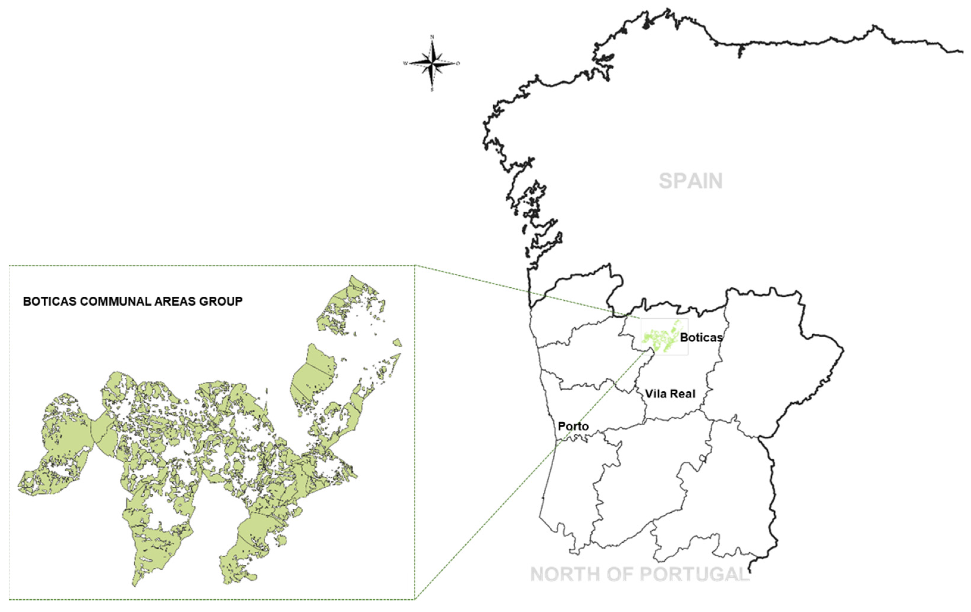
The study was carried out in pure Pinus pinaster forest, growing in the north of Portugal, in Tâmega’s river Valley, in the county of Vila Real, near the town of Boticas, in a group of communal areas. The common land in the municipality of Boticas represents 56% of the municipality area, which corresponds to 18,000 ha. In terms of land use, 52% of the area is forested (9500 ha), the predominant species being maritime pine, with pinewoods occupying around 7500 ha. In the municipality there are 26 common land units and 24 managing bodies. The partnerships established between various entities (ICNF, Forestis, Municipality of Boticas, the agrarian cooperative CAPOLIB, Cooperativa Agrícola de Boticas, and managing bodies of the common lands) allowed the constitution of a group of common lands with 22 units of common land and 20 management bodies. The group is designated as Boticas Communal Areas Group (“ADBaldios do Concelho de Boticas”, ABB). Location of ABB is represented in Figure 1. The entire group of communal area is located in the interval of 41°34′ N to 41°47′ N and 7°33′ W to 7°55′ W. The ABB occupies an area of 14,255 ha, which belongs to the national forest area of Perímetro Florestal do Barroso. Of the total area, 5014 ha correspond to pure maritime pine stands (Figure 2). These are mostly in areas with altitudes between 400 and 600 m. The maritime pine forests existing in this area are mainly managed for wood production. There are some stands in the study area, in which timber production is complemented by resin exploration, a non-timber and underutilized asset in this region.
The climate of the municipality of Boticas is described as a Sub-Atlantic climate with continental influences from Central Iberian Peninsula [32]. It presents an average annual temperature variation between 10 and 12.5 °C. In terms of annual precipitation, the values vary greatly throughout the area, from 600 mL in the Northeast to 2000 mL in the West, with air humidity ranging between 70 and 85%. Regarding the soil, the municipality of Boticas has two main types of soil, Rankers and humic Cambisols, predominantly from granite and schist [33]. The first type predominates in the areas with higher altitudes, to the north, and the latter in lower-altitude areas. In this case study, there was no relevant variation in the productivity of this species in conjunction with climate and soil in this location. However, it can be verified that this region of Tâmega’s river Valley presents edaphoclimatic characteristics conducive to productivity for this species with approximately 60% of the area classified as being of medium and/or superior site quality [34,35,36].
2.3. Stratification of Forest Cover and Forest Inventory
The classification and delineation of maritime pine strata and management plots were carried out with the support of aerial coverage of the study area (orthophoto maps of 2018) in ArcGis and QGIS environment. In the pine forest area, the stands were stratified through visual assessment according to an existing guidance protocol which contemplated 4 categories of density, based on the number of stems per hectare (N, trees ha−1) and 6 categories of age classes associated with the stage of development. Regarding density, the strata were defined as: Low (≤500 trees ha−1), Medium (501–1500 trees ha−1), High (1501–3000 trees ha−1), Very high (3001–10,000 trees ha−1), Extremely high (>10,000 trees ha−1). For the age, the following general classes were considered: Saplings (0–5 yr), Young-1 (6–12 yr), Young-2 (13–20 yr), Adult-1 (21–30 yr), Adult-2 (31–40 yr) and Mature (>40 yr). Information on fire history was used to support the assessment. Each stratum was then subdivided into homogeneous plots with individual areas of less than 10 ha, for forest management support purposes (management plots).
After the identification of the strata and the delimitation of the management plots, a forest inventory of 45 sample plots was carried out for the dendrometric characterization of the stands in the strata. The plots were randomly assigned within the strata, considering each stratum as an independent population. The number of plots per stratum varied according to stratum size. The plots were circular in shape and of 200 to 500 m2 in area, depending on the density class (with the lower areas for denser stands). The data collected in each plot refer to the diameter at breast height (d) of all living trees and total height (h) of a subsample of the trees. Additionally, evaluation of age and measurements of height were made for the dominant trees (using as a basis the largest 100 trees per hectare) for assessment of stand age and site index. The inventory results were also used to validate the stratification performed prior to the field work and support rectifications whenever deemed convenient. After collecting the field data, the stand typology was reclassified and allocation of the stands to strata were reviewed. A total of 23 different types of combinations were identified (Table 1).
The data supporting this study were extracted from the most representative plots of each of the different 23 combinations, from the sample of the 45 inventoried plots. Table 2 shows the statistical characterization for the stand variables evaluated in the representative stands. The information refers to stand age (t, years); number of trees (N, trees ha−1); stand basal area (G, m2 ha−1); site index (SI35, m); quadratic mean diameter (dg, cm). The variable ddom (cm) corresponds to the average diameter of the dominant trees and the average height of those dominant trees is the dominant height (hdom, m). Information on stand taper (hg/dg), as a measure of stability to wind, and canopy bulk density (CBD) related to crown fire potential is also shown.
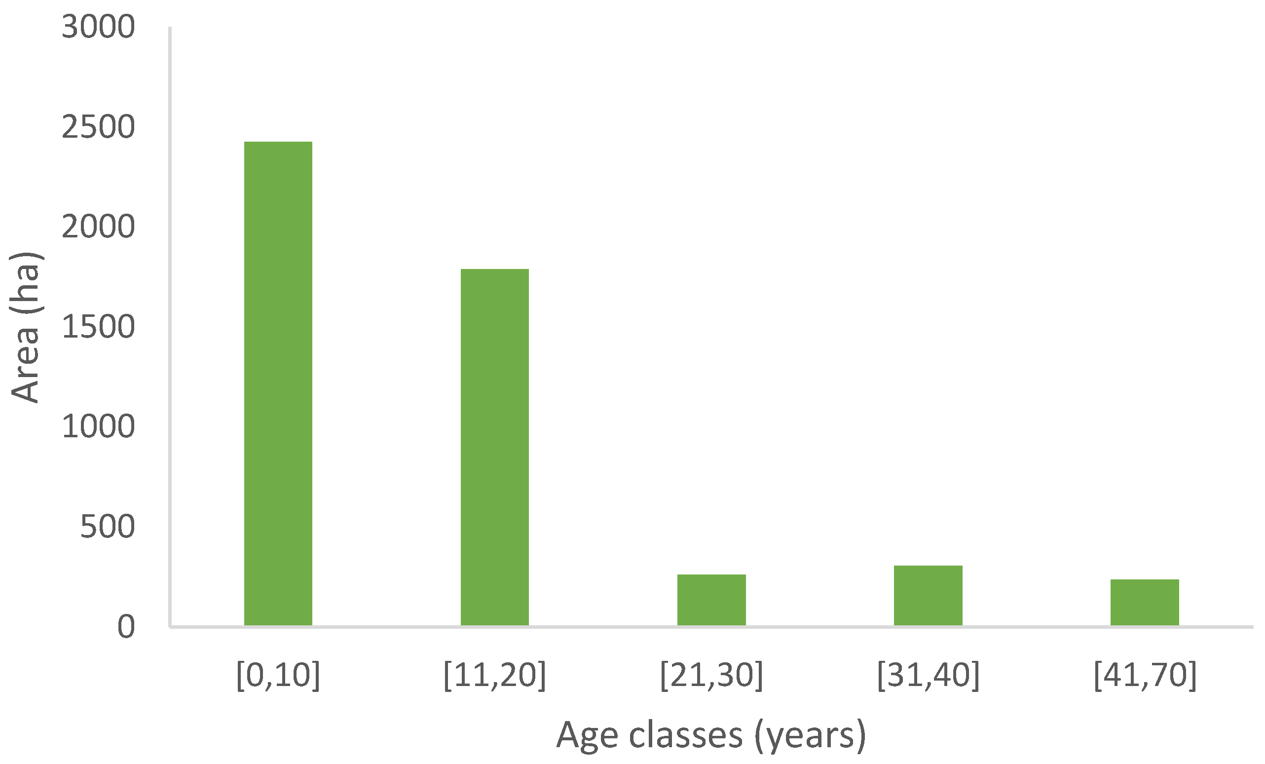
Figure 3 characterizes the distribution of the maritime pine stands area by 10-yr length age classes in the year of the forest inventory. The area for mature forests older than 41 years was aggregated into a single class due to its low representation in the study area.
2.4. Simulation of Growth Using ModisPinaster
Prediction of stand growth subject to specific management scenarios can be obtained with growth simulators. For this study, the authors selected ModisPinaster [27]. The simulator was developed using original supporting data collected on the overall region of Tâmega’s Valley maritime pine stands, where the case study is located. The simulator uses a reduced number of input data to run, based on typical forest inventory data (t, N, G, ddom, and hdom variables), and offers extensive output information. Briefly, ModisPinaster is a stand model with information disaggregation by diameter classes that allows the users to simulate the growth of the stands on an annual basis and thinning, during the period of simulation. The simulator incorporates two major management options of density regulation, as automatic or manual prescriptions, these being the stand density index (SDI, [37]) and the Wilson spacing factor (Fw, [38]). Alternatively, the user might decide to prescribe a thinning based on the specification of the number of trees to be removed or residual basal area. It also includes a mortality module that accounts for the effect of intra-species competition and damage associated with extreme weather events, such as windrow and uprooting. The simulator offers diverse information as output, such as stand volume, biomass (aboveground, per component, and root), carbon, and energy. ModisPinaster is available for free use, in a friendly interface, on the Computer Aided Projection of Strategies in Silviculture (CAPSIS) platform (http://www.inra.fr/capsis accessed on 17 May 2021) [39]. Comprehensive information about the model can be found in [22]. This simulator has been used in several case studies of forest management optimization (e.g., [1,4,40]) and to support the creation of accurate silvicultural models (e.g., [41,42]) for maritime pine.
The simulations of growth and thinning performed with the ModisPinaster took into account the regulation of density according to pre-specified values of the stand density index (SDI), as defined for maritime pine by [43]. In general, it was decided to maintain the density of the stands between 25% (beginning of competition) and 35% (lower limit of full occupancy). When the stand reaches a density index of 35%, the model simulates a selective thinning, from below, in order to lower the stocking to 25%. In cases of stands that initially had high densities, where this range was not suitable, the SDI ranges were fixed between 45% and 35%, adjusted to each specific case. For details on the key values of relative density, see [44].
For a set of four plots, where some interventions had already been decided, three different scenarios were additionally developed to follow the planned prescriptions. These cases correspond to young stands with high densities, regenerated from recurring forest fires that occurred at the site in previous years (cod_3; cod_7; cod_12; cod_17). The first thinning corresponds to a mechanical thinning, with a constant percentage removal of trees in each class of diameter, and the following are thinning from below. The intensity of the thinning from below was adjusted to assure specific regular spacing between trees.
Code 3 and 7 followed these guidelines:
- 1st thinning at 12 years, removing 27% of the existing trees;
- 2nd thinning at 20 years, reducing the density to 2000 trees ha−1 (2.5 m × 2 m);
- 3rd thinning at 27 years, reducing the density to 1666 trees ha−1 (2 m × 3 m);
- Evolution with SDI values ranging from 60% and 55% (near the lower limit of self-thinning).
Code 12 prescription:
- 1st thinning at 15 years, removing 27% of the existing trees;
- 2nd thinning at 15 years, reducing the density to 4444 trees ha−1 (1.5 m × 1.5 m);
- Evolution with SDI values in the range 45 and 30%.
Code 17 prescription:
- 1st thinning at 22 years, removing 27% of the existing trees;
- 2nd thinning at 22 years, reducing the density to 6667 trees ha−1 (1.5 m × 1 m);
- 3rd thinning at 27 years, reducing the density to 3333 trees ha−1 (1.5 m × 2 m);
- Evolution with SDI values 45 and 30%.
The authors selected the standing volume and the volume removed in thinning as input data in the optimization model (Section 2.5). In spite of some stands also being exploited for resin, this resource was not considered in this study, since, at this time, it is not yet a highly exploited asset in the area, with this consortium existing in just one common land unit in this group.
2.5. Optimization Model
This section presents the mixed integer formulation of the Forest Management Plan (FMP) problem. The goal is to determine where and when clear cutting should be undertaken in order to maximize the volume of wood harvested during the planning horizon considering silvicultural constraints, green-up constraints, sustainability constraints and operational constraints. In addition to clearcuts, thinning interventions are also carried out following the indications obtained by ModisPinaster.
The optimization model described in Section 2.5.1 refers to the main model, considering the grouping of areas and their owner bodies, hereafter designated as “global joint management”. In Section 2.5.2, information is provided on the modifications required to the main model and methodological steps followed to consider independent management, per common land, for the whole set of common lands. The latter approach is explicitly included to provide evidence on the research hypothesis being analysed about (the absence of) relevant differences in the volume of timber harvested or sustainability criteria when multi-stakeholder forest areas are managed as a whole or independently.
In order to solve the models, we used the optimization software Xpress 7.2 (available at http://www.fico.com/Xpress, accessed on 13 January 2022). Computations were performed on a computer equipped with an i5–2500 3.3 GHZ/3.7 Turbo CPU and 8 GB of RAM. The branch-and-bound algorithm was allowed to run for two hours at the most.
2.5.1. Global Joint Management
The following notation is used for the mathematical formulation.
Sets:
| set of one-year periods, where nt is the number of one-year time periods in the planning horizon, | |
| set of stands, where ns is the number of stands in the study area, | |
| set of common lands constrained to have incomes on periods, where nb is the number of these common lands, | |
| partition of set T in 5-year periods, | |
| subset of periods to impose constraints on age class area, | |
| set of periods to perform a thinning at stand , | |
| set of stands in common land i, | |
| the set of age classes, for each . |
Parameters:
| area of stand j (ha), | |
| age (years) of stand j in the first year of the planning horizon, | |
| timber volume obtained by clear-cutting stand j in period t (m3), | |
| timber volume obtained by thinning stand j in period t (m3), | |
| dominant height of stand j in period t, | |
| dominant height of stand j in period t, | |
| the quotient between and , | |
| tA | the target area, in ha, to each class of age, |
| Amax | the maximum area of a clearcut, |
| maximum number of years without incomes for a given set of common lands, BV, | |
| tol | years tolerance to perform a clearcut if stand has greater than 80, |
| M | big constant, |
| allowed margin for removed volume and area class age target, respectively. |
Variables:
| binary variable taking value 1 if a clear cutting is performed in stand j in period t and 0 otherwise, with , | |
| binary variable taking value 1 if an intervention is performed in common land in period t and 0 otherwise, with , | |
| integer variable representing the age, in years, of stand j in period t, with , | |
| binary variable taking value 1 if stand j in period t belongs to age class k and 0 otherwise, with . |
The mathematical model can be stated as follows:
Subject to:
The objective function (1) corresponds to maximizing the volume of timber harvested over the planning horizon.
Constraint (2) requires a clear-cut in the first period of the planning horizon in stands with an initial age of more than 70 years. Constraint (3) prevents clear-cuts in stands with less than 35 years old. Constraint (4) ensures that a maximum of one clear-cut is conducted on each stand during the planning horizon. Constraint (5) ensures a minimum time interval of five years between thinning and clear-cutting on each stand to allow a positive balance between expenditure associated with interventions and the return on the sales. It is worthwhile to mention that the period in which a thinning takes place is pre-defined, while the period to perform a clear-cut is not pre-defined in advance; it can occur over the entire planning horizon.
Constraint (6) prevents the formation of clear-cuts whose areas are greater than Amax, in the same year and the following two years, also ensuring the green-up period requirement, stated by path formulation [1,25]. In Portugal, the prescribed value for Amax is 10 ha. To formulate these constraints, consider set of all possible clusters that cannot be harvested at once in period t, with , and which are minimal. Each of these clusters is a contiguous group of stands whose total area exceeds Amax and which contains no similar cluster. That is, if one stand is excluded from this cluster, the remaining could be cut at once. Therefore, if r is the number of stands in such a cluster, then the number of stands in that cluster that can be harvested during the green-up period (3 years) is at most r − 1. It should be noted that two stands are adjacent when they both share a boundary that is not a discrete set of points. The minimal infeasible clusters were obtained recursively. One starts from clusters with only one stand, in which one stand is gradually added each time until the maximum area is exceeded.
Constraint (7) aims to ensure the stability of the stands by imposing the clear-cutting of stands in the period where the quotient between hg and dg exceeds the wind instability threshold of 80 or in the following tol periods, as long as it is within the planning horizon.
Constraints (8) and (9) ensure that there is revenue in each tv-year period for the set of BV common lands. Constraint (8) links variables and , ensuring that if in period t there is clear-cutting or thinning in at least one stand of common land i, then variable takes value 1; otherwise, it takes the value 0. Constraint (9) ensures revenue for any period of tv consecutive years.
Constraints (10) and (11) assure balanced volume revenue considering 5-year periods by imposing that the relative difference in volume removed between two consecutive 5-year periods does not exceed Δ.
Constraints (12)–(15) establish conditions on the age structure of the forest. Constraint (12) defines the age of each stand at every period, and constraints (13) and (14) state the age class that stand j belongs to for each period, where takes value 1 if stand j in period t belongs to age class k and 0 otherwise. Constraints (15) ensure, for every period in a given set of periods, that the area in each age class is within and times the target area for each class, .
Finally, constraints (16)–(18) establish the domain of the variables.
To evaluate the impact of some groups of constraints, variations of the presented model are considered where only some constraints are included. Table 3 briefly describes the considered models. The base model, FMPb, includes only the clear-cut area constraints and the silvicultural constraints, which guarantee the clear-cutting of plots at convenient ages. The FMPs model is obtained by additionally considering the forest stability constraints. The FMPr model is obtained by considering the revenue constraints for a set of common lands, and the FMPv model is obtained by including the balanced volume revenue constraints. The FMPy model is obtained including the age class structure constraints, and FMP denotes the model with all constraints.
2.5.2. Independent Management, Per Common Land
The main model presented in the previous section can be easily adapted to consider the independent management per common land. The set of stands , in this case, will be restricted to the stands of the common land under consideration. The objective function (1) and the set of constraints from (2) to (19) are maintained, bearing in mind the new set of stands. However, for constraint (6), it was necessary to calculate, for each common land, the corresponding set of all possible clusters that cannot be harvested at once in period t, with , and which are minimal. Constraints (8) and (9) are only included for the common land under consideration.
2.6. Statistical Analysis—Comparison among Models
The results achieved with the formulations described in Section 2.5.1 (global management—FMP model) and Section 2.5.2 (independent management, per common land) were statistically compared to study the validity of the base hypothesis of non-significant differences among models. Only 18 of the 22 common lands in the study area were considered, in this statistical analysis, because the dimension of the other four did not lead to feasible solutions with independent management. We have paired observations of the form (, ) for a set of common lands, referring to the predicted value provided by one approach and the value obtained with the other. We are interested in testing under the null hypothesis that the differences = are equal to zero. Two variables were considered, each at once, in testing: (i) the values of volume and (ii) the average stand age at the end of the planning period. The appropriate test for matched pairs depends on the data characteristics, specifically on the assumption of normality. If the data met the assumption of normality, the t-test on paired samples was recommended. To account for an eventual deviation to normality, evaluated with the Shapiro–Wilk test, we considered the use of the nonparametric Wilcoxon signed-rank test [45]. All the statistical tests were performed with SPSS software (IBM SPSS Statistics 26).
3. Computational Results
In this section, the computational experiments are described, and the obtained results are analysed for the study area.
3.1. Used Parameters and Constraints
This section presents some remarks about the values considered for the model parameters and additional adjustments to comply with independent management.
The complete description of the parameters is presented in Section 2.5. and the used values are stated in Table 4.
To get feasible problems, constraint (15) is only included for the last period of the planning horizon, , due to the age structure of the study area. Furthermore, the target area, is a fifth of the total area (since there are five age classes) and = 0.5.
It was considered tv = 5 for the maximum number of years without incomes for the B set of common lands. An attempt was made with a lower value, but this was the one that led to a feasible problem. The value 186 for the big constant M was chosen because it should be an upper bound on the number of stands, by common land, that could be harvested during tv-years, and the maximum number of stands in a common land is 186.
In the last age class in K, the upper limit of 70 is considered because it corresponds to the maximum age allowed, by which time the mandatory cutting is imposed.
Regarding the tol parameter, constraint (7), it should be noted that there was a need to relax the clear-cut date due to the clear-cut area constraints because there are several adjacent stands with similarly high values for the quotient . After several computational tests, to get a feasible model, a margin of tol = 8 years was considered. The information about the set of periods, , to perform a thinning on each stand j is obtained from ModisPinaster and is given data for the model.
On constraint (10), six 5-year periods, T1, ⋯, T6, and were considered, values that enable the optimal solution to be found with acceptable variations in the volume of wood removed.
Concerning the adjustments to comply with independent management, notice that the adaptation of the global joint management model to the independent management situation was carried out in steps, starting with the base model and adding the defined constraints to reach the most complete model possible. The computational experiments with the independent management per common land revealed a further need to adjust and drop some constraints. Only the base model, FMPb, allows for obtaining feasible solutions. Depending on the characteristics of the common land being considered, it might not be possible to ensure the regularity of revenue, constraint (10), and the constraint of the age classes at the end of the planning horizon, constraint (15). For the case study, after a preliminary test, which showed that it was only possible to include such constraints for a reduced number of common land, it was decided to drop constraint (10) and include an age-related sustainability constraint, assuring that the final average age should be at least 20 years, stated as follows:
where represents the age, in years, of stand j in the last year of the planning horizon, nt and represents the area of stand j.
So, the characteristics of the common land under consideration in the case study, namely the number of stands and their age distribution, dictated the set of constraints to be included. Two models are, therefore, considered the base model (FMPb), as originally defined in Table 4, hereafter denoted as FMPb-IND, and a version of the FMP model, FMP-IND. Both models are presented in Table 5.
3.2. Obtained Results
Table 6 presents the number of variables and constraints of the various models presented under the Global joint management approach, as well as information about the performance of the branch-and-bound algorithm (execution time and final gap) and the optimal value. The gap associated with a solution is the relative difference between its objective function value and the best majorant determined so far. All the runs stopped before the time limit considered, 7200 s, so the final relative gap is 0.0% for all the models.
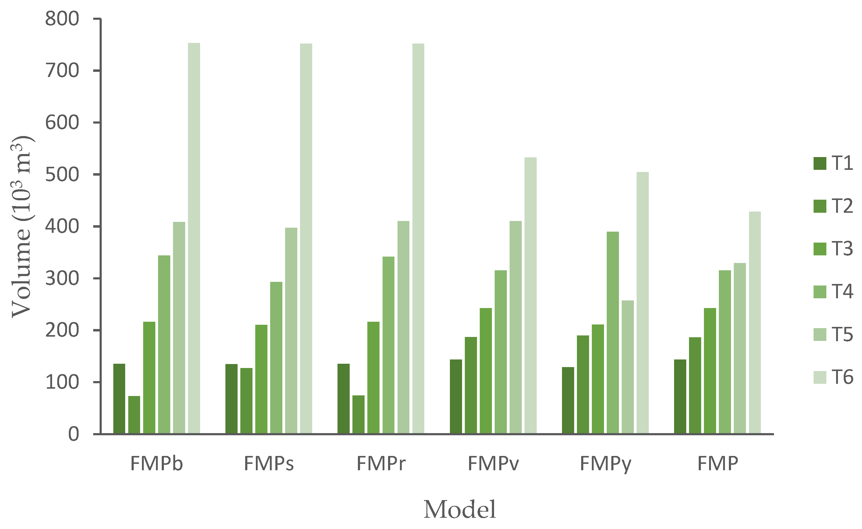
In Figure 4, a bar chart is presented, showing the volume of timber removed, in each five-year period during the planning horizon for the models identified in Table 3.
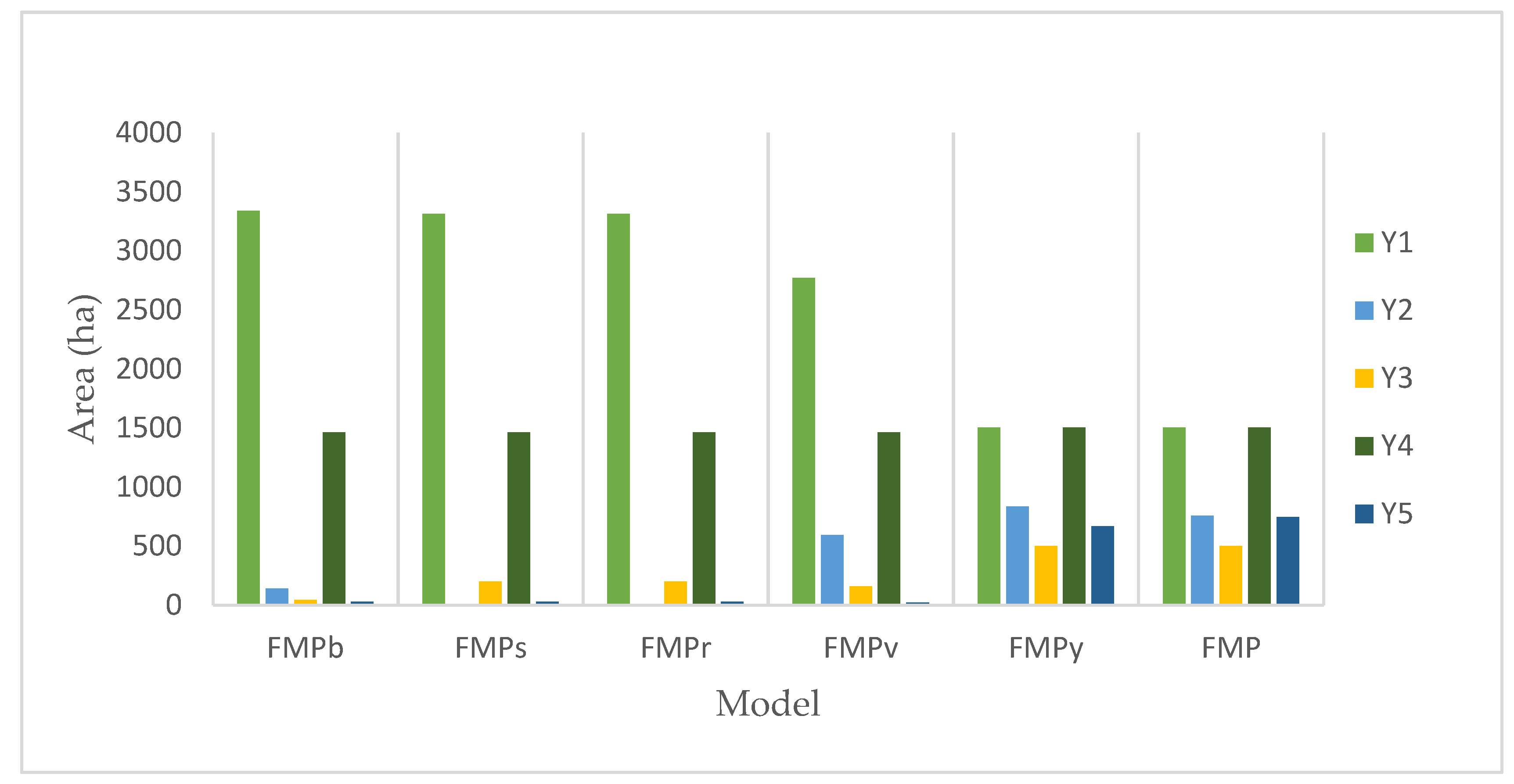
Figure 5 characterizes the area distribution among age classes in the last year of the planning horizon, for the six models.
As can be seen in Figure 4 and Figure 5, the optimal solutions obtained for the FMPb, FMPr and FMPs models are quite similar in terms of volume removed and the area occupied per age class in the last year of the planning horizon. Hereafter, of these three models, only results for the base model (FMPb) will be presented. In Table 7, the optimal solutions for the FMPb, FMPv, FMPy and FMP models are characterized, in terms of the volume removed by clear-cutting and thinning, and the total volume removed over the planning horizon.
In Table 8, the average stand age at the end of the planning horizon is characterized for the models FMPb, FMPs, FMPr, FMPv, FMPy and FMP. The value of average age is given by Equation (21).
In addition to the results presented for the global joint management models, identified in Table 3, computational results were obtained considering the two individual management models, identified in Table 5, models FMPb-IND and FMP-IND. Of the 22 common lands in the study area, four were not considered in the individual management approach due to their small size or existing areas of dispute.
In Table 9, the optimal solutions for models FMP and FMP-IND are characterized, in terms of the number of stands and areas to undertake clear-cut and thinning, by each 5-year period of the planning horizon. To allow a direct comparison between the individual and global joint management approach, the authors restricted the presentation of the results for the same 18 common lands, extracted from the solution obtained with the joint global management model FMP (Table 3) for the entire set of 22 common lands. The small size of the other four common lands did not allow for admissible solutions with independent management, and they were, therefore, not considered.
Table 10 shows the values of the total volume (m3) removed throughout the planning period, the final average age of the stands for the models FMPb-IND and FMP-IND, and the relative variation with both management approaches, using the results attained with the global joint management as a basis for comparison, for the same 18 common lands.
Investigation of statistically significant differences in the harvested volume of timber and on the distribution of stand age with multi-stakeholder forest areas, managed independently (I) or when they are managed as a whole (G), was performed as described in Section 2.6. For the removed volume, the Shapiro–Wilk test showed the variable did not assume normality (test statistic = 0.694, p-value = 0.000), hence the Wilcoxon single-rank test was applied. The Wilcoxon signed-rank test showed that the global forest area’s management elicited a statistically significant change in the harvested volume with independent management (Z = −3.375, p-value = 0.001). For the variable average age at the end of the planning horizon, the assumption of normality was met for the differences variable (test statistic = 0.903, p-value = 0.065). The t-test (t = −0.657, p-value = 0.520) and the Wilcoxon signed-rank test (Z = −0.631, p-value = 0.528) showed no statistical differences for the average ending age variable of both models (whole management versus independent management) at the end of the planning horizon.
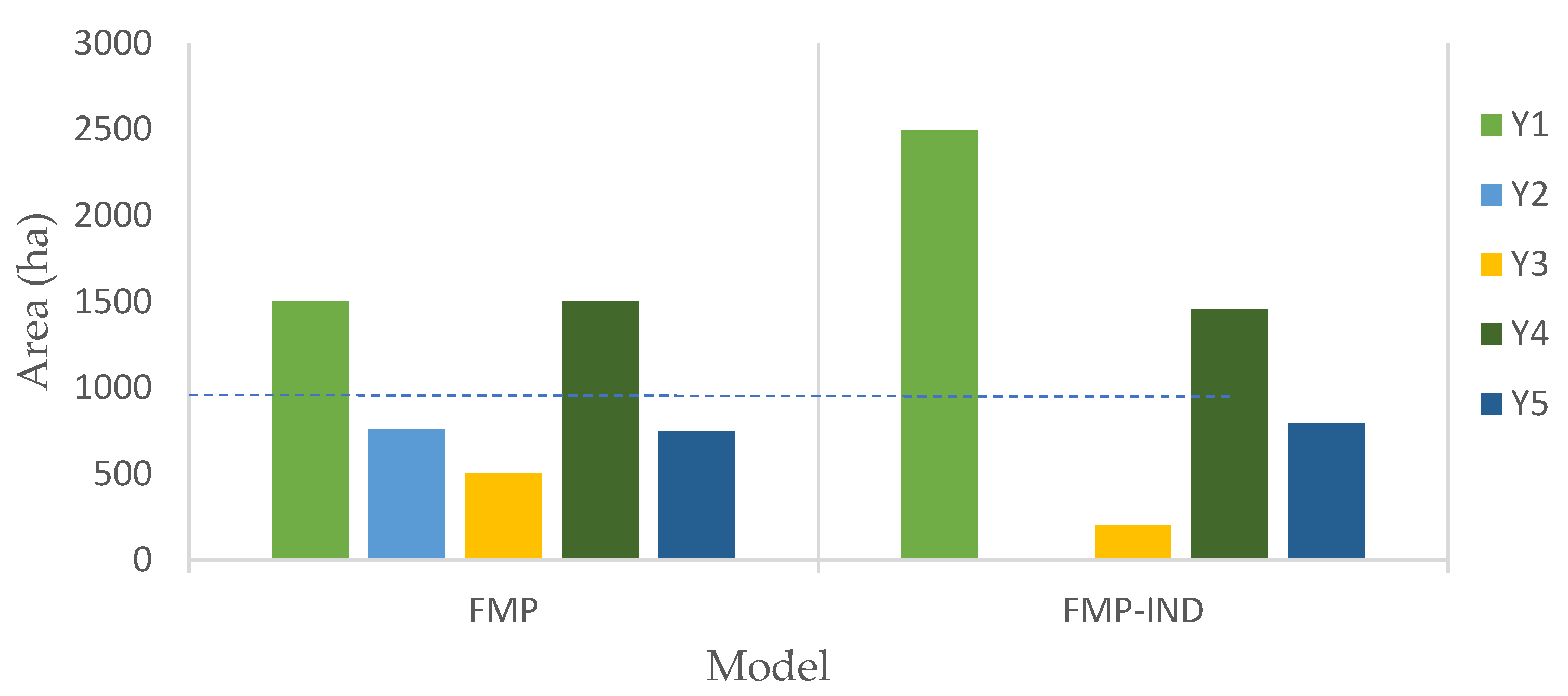
Figure 6 presents the area distribution among age classes in the last year of the planning horizon for the FMP model, considering the global management (also depicted in Figure 5) and for the FMP model when the management is individualized (FMP-IND). In the case of the FMP model, the total area under analysis is 5014 ha, while for the FMP-IND, the total area is 4944 ha, due to the exclusion of 4 common lands out of the 22, with a reduced area of pine forest. The dotted line in Figure 6 represents the average value corresponding to a balanced distribution of the area of common land by age class, set at 1000 ha, to help visualize the differences.
4. Discussion
Based on the results presented in Section 3, in particular in Table 6, Table 7, Table 8, Table 9, Table 10 and Figure 4 and Figure 5, it can be concluded that the base model corresponds to a greater volume of removed timber, 1,928,699.5 m3. This corresponds to the expected outcome, due to the lower number of constraints included in this base version (Table 3). The inclusion of stability constraints, FMPs model, leads to a slight reduction in the amount of timber volume harvested (0.76%). A negligible reduction of 0.04% also occurs when the constraints on the revenues per common land, FMPr, are included. The other set of constraints has a greater impact on the reduction in the removed volume, being 5.1% in the model FMPv, 12.89% in model FMPy and 14.76% in model FMP.
Although the total volume of harvested wood is smaller over the planning horizon with the FMP model (1,643,956.8 m3), this model provides a result that is most consistent with the sustainable management of the forests. In the FMP model, the three pillars of sustainability—environmental, economic and social—are addressed. Examples of environmental issues considered in the model are the forest stability and the assurance of a more balanced age class distribution in the area. The achievement of a balanced volume income during the planning horizon, matching the preferences of local entities with guaranteed revenue per vacant land in each 5-year period, directly relates to economic value and social preferences.
The increase in the average stand age at the end of the planning horizon (a value higher than 22 years with the FMP model, see Table 9) is an additional element confirming the better adjustment to sustainable management criteria achieved with this model. As shown in Figure 3, at the beginning of the planning horizon, the distribution of maritime pine stands by age classes is not balanced. The main reason is the occurrence of frequent (and recurrent) forest fires that have affected the studied region. The forest inventory shows that 84% of the stands in the study area are up to 20 years old (corresponding to natural regenerated areas after forest fires) and the remaining 16% corresponds to stands with age values greater than 20 years. This imbalance greatly conditioned the set of periods, in which balanced distribution by age classes is guaranteed, (15). In order to obtain feasible problems, it was only practicable to include this set of constraints at the end of the planning horizon, that is, only, , was considered, which will facilitate management in later periods. During the planning horizon, the volume regularity already guarantees revenues throughout the planning period.
Some authors [4] include restrictions that limit the final average age. In this work, we have chosen not to include such constraints. Although the constraints that limit the average final age, inferiorly, are not included, the values presented in Table 9 allow us to conclude that constraint (15), in addition to ensuring the most balanced distribution by area classes, leads to satisfactory values of the final age, 19.94 for the model FMPy and 22.28 for FMP. Without constraint (15), the average age at the end is very low, ranging from 10 to 15 years (models FMPb, FMPs, FMPr and FMPv). The value of stand age equal to or lower than 15 years does not fit with the typical rotation values proposed for the species, even when considering a shorter rotation length which, is around 20 years [4,41].
In the optimal solution of the base model, FMPb, Table 8, 89% of the clear-cutting area is cut in the last two 5-year periods. With the FMP model, the total area subjected to clear-cut decreases compared to FMPb. Furthermore, although in the later years the total clear-cut area is larger, the difference is not so substantial, in the last two 5-year periods, clear-cutting corresponds to about 55% of the total clear-cut area.
The results obtained for the group of 22 common lands confirm the usefulness of linear programming-based optimization models to accommodate multiple owners. In terms of flexibility to accommodate changes or to be applied to other areas, the mathematical model presented in Section 2.5 is generic enough to be easily adaptable to account for stands of various stages of development and stand densities. For the case study, high density values were identified in early stages, which is in accordance with the maximum attainable density trajectory for the species presented by [46]. Those values were accounted for in the simulations performed with ModisPinaster and considered in the optimization model.
Generalization to other forest systems can be easily accommodated. For example, considering another species with different conditions to perform a final cut should adapt constraints (2) and (3). Further, the wind instability in constraint (7) could be different for other species.
The mixture of several forest species can also be easily contemplated. Constraints (2)–(5) impose conditions for carrying out clear-cutting, and should be adjusted to the species under study. Constraint (6), which prevents the formation of clearings with more than 10 ha, with an exclusion period of two years, should cover all stands, regardless of the forest species. In constraint (7), which ensures the stability of the stands, the threshold value considered for the quotient between average height and diameter must be adjusted for each of the species under study. Constraints (8) and (9), which ensure revenues per each common land, must include all the plots of it. Constraints (10) and (11), which assure balanced volume revenue, must include all the study area, regardless of the species. Constraints (12)–(15), which establish conditions on the age structure of the forest, should be adapted for each species.
The crown fire potential effect, evaluated through the variable canopy bulk density (CBD), can be easily added, in constraint similar to constraint (7), used for tree stability. For the case study, its use was not considered in the models because the majority of the stands had values of CBD higher than the threshold limit of 0.08 (km/ kg/m3) [47]. Development should extend the optimization problem to account the broad role and multiple functions of forests, such as the production of resin and carbon sequestration. The effect of disturbances, such as pests and diseases, can also be handled with this optimization approach for forest management planning.
With this research, the authors also aimed to analyse the effect of grouping areas (with different owner bodies), compared to independent management, in terms of sustainability. The criteria used for the assessment are the total volume removed over the planning horizon and the regularization of the age of the forests at the end of the planning period. Examination of the effect of the set of constraints was also performed. Comparing the results obtained in individual management and global management with the base model (FMPb and FMPb-IND, global results provided in Table 10), the following remarks should be highlighted:
As expected, the volume removed per common land area either coincides or is lower with global management. This is because, in the global management scenario, the clearing constraints consider adjacencies between patches that are distinct vacant areas and, therefore, the clearing constraints become more restrictive. In this case study, the reduction in volume occurred in only four fallow patches, with reduction values between 0.2% and 1.6%.
The total removed volume with global management, in the 18 common lands, was reduced by about 0.2%, corresponding to 4242 m3 during the 30 years of the planning horizon.
The average final age of the common land varies in both individual and global management scenarios, between 0.9 and 26.2 years (data per common land not shown), presenting a minor positive difference, when considering all of the common lands ( around 10 years, Table 10).
It should be noted that the authors do not advocate the use of the base model, FMPb, for forest managers to follow. The FMPb model is a reference point, where the constraints that must be considered (silvicultural and green-up) are considered, highlighting the importance of guaranteeing sustainability and operational constraints. The average final age achieved with the optimal solution is particularly low, which compromises the future management of the study area.
The comparison of the results obtained by individual and global management with the complete model must be done with caution (FMP and FMB-INV, global results provided in Table 10), but does not prevent the highlighting of important patterns accounted for by the management mode. As mentioned before, it was necessary to make adjustments to the individual management model to obtain feasible solutions. In the global management model, FMP, constraints on the area by classes of age ensure reasonable values for the average final age of the whole study area, 22.28 years, as well as a better balance of area per age class (Figure 6). When analysing the final average age per common land, it varies between 15.6 and 38.2 years. For individual management, because of the constraints bounding average final age to at least 20 years, common land’s average final age varies between 20 and 26.2 years. As far as volume is concerned, the results achieved with the global management optimal solution show a reduction in total wood harvested over the 30-year planning horizon, in the order of 140,000 m3, 8.6% in a relative basis (Table 10). This difference has proved to be statistically significant (p = 0.000). The analysis made per common land shows a variation from −20% to +2.9%, regarding the results obtained with the FMP model, compared to the FMP-IND model.
The option for global management is more interesting than individual management, in terms of guaranteeing the sustainability of resources, even though a compromise is implicit between the reduction in the amount of wood that is cut and what is gained in the medium term, in terms of resource sustainability.
The proposed model is replicable and recommendable for other clustering situations, either of communal areas or of areas belonging to multiple private owners, under a private governance model. Examples of the latter occur in Eastern European countries, where private forest ownership is often highly fragmented, with properties of small size, after the restitution of landownership [48]. As stated in the FAO study, forest owners’ organizations, such as forest owners’ associations and forest owners’ cooperatives, are an instrument for supporting the sustainable management of private forests. The use of optimization models, such as the FMP developed in this study, can easily help with this aim.
5. Conclusions
This work considers a relatively long planning horizon, 30 years, in a large group of communal areas, involving diverse management bodies, where the decision of the period in which clear-cutting and thinning takes place is provided by the optimal solution of the optimization model. The proposed optimization model takes into account the specific silvicultural constraints of maritime pine species and is consistent with the specification of the problem that was intended to be studied: it ensures sustainable management with a balanced age classes structure at the end of the planning horizon; it includes constraints on the maximum area of clearings; it ensures balanced revenues of volume over all the study area and regular revenues per common land that meet the interests of the communities; it considers the stability factor that allows the management plan to be adjusted, taking into account susceptibility to wind damage, associated with climate change and beyond that, it can be used or adapted to other regions, regardless of species, and to other groups of areas with multiple managing bodies, such as the ones occurring with implementation of associativism. To the best knowledge of the authors, assessment of the impact of changing governance policies in the management of forest areas has never been accomplished for real cases of study, involving common lands in Europe.
When comparing the type of management, individual or global, the global joint management approach, supported by the FMP optimization model, presented a noticeable reduction of around 8.6% in removed volume and a higher value of age for the existing stands at the end of the planning horizon, compared to the model that considers individual management (FMP-IND model). It should be noted that individual management does not guarantee environmental restrictions of the stands, assured with global management, because at the spatial level, there are patches with continuity between the commons, jeopardizing the landscape structure, and translating into possible impacts on the ecosystem.
It can be concluded that global management, when compared to individualized management, implies a trade-off between the wood harvested, which is reduced in the former, and what is gained, in the medium term, in resource sustainability, as proven by the increase in the average age of the remaining stands at the end of the planning period in the latter.
Author Contributions
Conceptualization, all the authors; methodology, all the authors; software, all the authors; formal analysis, all the authors; investigation, all the authors; resources, A.C. and T.F.F.; writing—original draft preparation, all the authors; writing—review and editing, all the authors; supervision, A.C. and T.F.F. All authors have read and agreed to the published version of the manuscript.
Funding
The participation of the co-author Adelaide Cerveira was financed by National Funds through the Portuguese funding agency, FCT-Fundação para a Ciência e a Tecnologia, within project: LA/P/0063/2020. The participation of the co-author Teresa Fonseca was financed by the Forest Research Centre, a research unit funded by Fundação para a Ciência e Tecnologia I.P. (FCT), Portugal (UID/ 00239/2020).
Institutional Review Board Statement
Not applicable.
Informed Consent Statement
Not applicable.
Data Availability Statement
The data are not publicly available.
Acknowledgments
The authors thank CAPOLIB, in particular, Ângelo Teixeira, Miguel Alves and Francisco Fernandes, for providing support with the case study. We thank, also, Carlos Fernandes and Nuno Ferreira, for their collaboration on the forest inventory.
Conflicts of Interest
The authors declare no conflict of interest.
References
- Fonseca, T.F.; Cerveira, A.; Mota, A. An integer programming model for a forest harvest problem in Pinus pinaster Stands. For. Syst. 2012, 21, 272–283. [Google Scholar] [CrossRef] [Green Version]
- Pohjanmies, T.; Triviño, M.; Tortorec, E.L.; Salminen, H.; Mönkkönen, M. Conflicting objectives in production forest pose a challenge for forest management. Ecosyst. Serv. 2017, 28, 298–310. [Google Scholar] [CrossRef] [Green Version]
- Álvarez-Miranda, E.; Garcia-Gonzalo, J.; Ulloa-Fierro, F.; Weintraub, A.; Barreiro, S. A multicriteria optimization model for sustainable forest management under climate change uncertainty: An application in Portugal. Eur. J. Oper. Res. 2018, 269, 79–98. [Google Scholar] [CrossRef]
- Costa, P.; Cerveira, A.; Kašpar, J.; Marušák, R.; Fonseca, T.F. Forest Management of Pinus pinaster Ait. in Unbalanced Forest Structures Arising from Disturbances—A Framework Proposal of Decision Support Systems (DSS). Forests 2021, 12, 1031. [Google Scholar] [CrossRef]
- Clutter, J.L.; Fortson, J.C.; Pienaar, L.V.; Brister, G.H.; Baily, R.L. Timber Management: A Quantitative Approach; John Wiley and Sons: New York, NY, USA, 1983; p. 333. [Google Scholar]
- Murray, A.T. Spatial restrictions in harvest scheduling. For. Sci. 1999, 45, 45–52. [Google Scholar] [CrossRef]
- Martins, I.; Constantino, M.; Borges, J.G. Forest Management Models with Spatial Structure Constraints; CIO/Faculdade de Ciencias de Lisboa: Lisbon, Portugal, 1999. [Google Scholar]
- McDill, M.E.; Rebain, S.A.; Braze, J. Harvest scheduling with area-based adjacency constraints. For. Sci. 2002, 48, 631–642. [Google Scholar] [CrossRef]
- Murray, A.T.; Weintraub, A. Scale and unit specification influences in harvest scheduling with maximum area restrictions. For. Sci. 2002, 48, 779–789. [Google Scholar] [CrossRef]
- Crowe, K.; Nelson, J.; Boyland, M. Solving the area-restricted harvest-scheduling model using the branch and bound algorithm. Can. J. For. Res. 2003, 33, 1804–1814. [Google Scholar] [CrossRef]
- Martins, I.; Constantino, M.; Borges, J.G. A column generation approach for solving a non-temporal forest harvest model with spatial structure constraints. Eur. J. Oper. Res. 2005, 161, 478–498. [Google Scholar] [CrossRef]
- Goycoolea, M.; Murray, A.T.; Barahona, F.; Epstein, R.; Weintraub, A. Harvest scheduling subject to maximum area restrictions: Exploring exact approaches. Oper. Res. 2005, 53, 490–500. [Google Scholar] [CrossRef] [Green Version]
- Vielma, J.P.; Murray, A.T.; Ryan, D.M.; Weintraub, A. Improving computational capabilities for adressing volume constraints in forest harvest scheduling problems. Eur. J. Oper. Res. 2007, 176, 1246–1264. [Google Scholar] [CrossRef] [Green Version]
- Constantino, M.; Martins, I.; Borges, J.G. A new mixed-integer programming model for harvest scheduling subject to maximum area restrictions. Oper. Res. 2008, 56, 542–551. [Google Scholar] [CrossRef]
- Goycoolea, M.; Murray, A.T.; Vielma, J.P.; Weintraub, A. Evaluating approaches for solving the area restricted model in harvest scheduling. For. Sci. 2009, 55, 149–165. [Google Scholar] [CrossRef]
- Martins, I.; Alvelos, F.; Constantino, M. A branch-and-price approach for harvest scheduling subject to maximum area restrictions. Comput. Optim. Appl. 2012, 51, 363–385. [Google Scholar] [CrossRef]
- Borges, P.; Martins, I.; Bergseng, E.; Eid, T.; Gobakken, T. Effects of site productivity on forest harvest scheduling subject to green-up and maximum area restrictions. Scan. J. For. Res. 2016, 31, 507–516. [Google Scholar] [CrossRef]
- Hoen, H.F.; Eid, T. A Model for Analysis of Treatment Strategies for a Forest Applying Standvice Simulations and Linear Programming; Norwegian Forest Research Institute: Espeland, Norway, 1990; p. 35. [Google Scholar]
- Raymeret, A.K.; Gobakken, T.; Solberg, B.; Hoen, H.F.; Bergseng, E. A forest optimisation model including carbon flows: Application to a forest in Norway. For. Ecol. Manag. 2009, 258, 579–589. [Google Scholar] [CrossRef]
- Finney, M.A. Design of regular landscape fuel treatment patterns for modifying fire growth and behavior. For. Sci. 2001, 47, 219–228. [Google Scholar] [CrossRef]
- León, J.; Reijnders, V.M.; Hearne, J.W.; Ozlen, M.; Reinke, K.J. A landscape-scale optimisation model to break the hazardous fuel continuum while maintaining habitat quality. Environ. Model. Assess. 2019, 24, 369–379. [Google Scholar] [CrossRef]
- Fonseca, T.F.; Parresol, B.; Marques, C.; de Coligny, F. Models to Implement a Sustainable Forest Management—An Overview of the ModisPinaster Model. In Sustainable Forest Management/Book 1; Martín, J.G., Diez Casero, J.J., Eds.; InTech-Open Access Publisher: London, UK, 2012; pp. 321–338. [Google Scholar]
- Cerveira, A.; Fonseca, T.; Mota, A.; Martins, I. An Integer Programming Model for the Management of a Forest in the North of Portugal. In Numerical Analysis Applied Mathematics ICNAAM 2011: International Conference on Numerical Analysis and Applied Mathematics; Simos, T.E., Psihoyios, G., Tsitouras, C., Anastassi, Z., Eds.; AIP: Melville, NY, USA, 2011; pp. 1890–1893. [Google Scholar]
- Vopěnka, P.; Kašpar, J.; Marušák, R. GIS tool for optimization of forest harvest-scheduling. Comput. Electron. Agric. 2015, 113, 254–259. [Google Scholar] [CrossRef]
- Martins, I.; Cerveira, A.; Mota, A.; Bento, J.; Fonseca, T. Sustainable Management of a Northern Portugal Forest, Recent Re-searches in Environment, Energy Systems and Sustainability. In Proceedings of the 8th WSEAS International Conference on EEESD’12, Faro, Portugal, 2–4 May 2012; Ramos, R.A.R., Straupe, I., Panagopoulos, T., Eds.; WSEAS Press: Algarve, Portugal, 2012; pp. 232–237. [Google Scholar]
- Government of Portugal. 2019. Available online: https://www.portugal.gov.pt/en/gc21/comunicacao/noticia?i=government-finances-criacao-de-agrupamentos-de-baldios (accessed on 4 December 2021).
- Fonseca, T.F. Modeling the Growth, Mortality and Diametric Distribution of Maritime Pine Forest in the Tâmega Valley (Modelação do Crescimento, Mortalidade e Distribuição Diamétrica do Pinhal Bravo no Vale do Tâmega). Ph.D. Thesis, Universidade de Trás-os-Montes e Alto Douro, Vila Real, Portugal, 2004. [Google Scholar]
- ICNF. Portugal Perfil Florestal. Available online: https://fronteirasxxi.pt/wp-content/uploads/2021/06/ICNF_Perfil-Florestal_v31_01_2021.pdf (accessed on 7 December 2021).
- Bica, A.; Carvalho, A. Os Baldios e o Regime Florestal—Uma Questão a Resolver; BALADI—Federação Nacional dos Baldios: Vila Real, Portugal, 2021; pp. 1–75. [Google Scholar]
- Skulska, I.; do Loreto Monteiro, M.; Rego, F.C. Gestão dos terrenos comunitários. Análise dos planos de utilização dos baldios. Silva Lusit. 2020, 28, 126–128. [Google Scholar] [CrossRef]
- Coelho, I.S. Propriedade da terra e política florestal em Portugal. Silva Lusit. 2003, 11, 185–199. [Google Scholar]
- PERUVB. Programa Estratégico de Reabilitação Urbana da Vila de Botica—Relatório de Caracterização e Diagnóstico; Sociedade Portuguesa de Inovação: Porto, Portugal, 2016; pp. 15–16. [Google Scholar]
- Atlas do Ambiente. Atlas Digital do Ambiente. Agência Portuguesa do Ambiente. SNIAmb. Informação Geográfica. Available online: https://sniamb.apambiente.pt/content/geo-visualizador?language=pt-pt (accessed on 14 October 2021).
- Aranha, J.T. Na Integrated Geographical Information System for the Vale do Alto Tâmega (GISVAT). Ph.D. Thesis, Kinston University, Kinston, NC, USA, 1998; p. 327. [Google Scholar]
- Marques, C.P.; Fonseca, T.F.; Aranha, J.T.; Duarte, J.P.C.; Ribeiro, E.L.; Duro, M.R.; Brás, M.J. Ordenamento de Povoamentos de Pinheiro-Bravo na Região do Alto Tâmega; Relatório Final do Projeto PAMAF 4004; Universidade de Trás-os-Montes e Alto Douro: Vila Real, Portugal, 2000. [Google Scholar]
- ICNF. Programa Regional de Ordenamento Florestal de Trás-os-Montes e Alto Douro-Capítulos A, B e C; Documento Estratégico; ICNF: Lisboa, Portugal, 2019. [Google Scholar]
- Reineke, L.H. Perfecting a stand-density index for even aged forests. J. Agric. Res. 1933, 46, 627–639. [Google Scholar]
- Wilson, F.G. Numerical expression of stocking in terms of height. J. For. 1946, 44, 758–761. [Google Scholar]
- Dufour-Kowalski, S.; Courbaud, B.; Dreyfus, P.; Meredieu, C.; de Coligny, F. Capsis: An open software framework and com-munity for forest growth modelling. Ann. For. Sci. 2012, 69, 221–233. [Google Scholar] [CrossRef]
- Mota, A.A.R. Exploitation Plan for Pinus pinaster Ait. in the Ribeira de Pena Forest Reserve, Barroso Forested Area (Plano de Exploração para Pinus pinaster Ait. dos Baldios de Ribeira de Pena, Perimetro Florestal do Barroso). Master’s Thesis, Universidade de Trás-os-Montes e Alto Douro, Vila Real, Portugal, 2011. [Google Scholar]
- Fonseca, T.F.; Lousada, J.L. Management of Maritime Pine: Energetic Potential with Alternative Silvicultural Guidelines. In Forest Biomass—From Trees to Energy; Gonçalves, C., Sousa, A., Malico, I., Eds.; InTech-Open Access Publisher: London, UK, 2021; pp. 71–86. [Google Scholar]
- Fonseca, T.F.; Duarte, J.C. A silvicultural stand density model to control understory in maritine pine stands. iFlorest 2017, 10, 829–836. [Google Scholar] [CrossRef] [Green Version]
- Luis, J.S.; Fonseca, T.F. The allometric model in the stand density management of Pinus pinaster in Portugal. Ann. For. Sci. 2004, 61, 807–814. [Google Scholar] [CrossRef] [Green Version]
- Long, J. A practical approach to density management. For. Chron. 1985, 61, 23–27. [Google Scholar] [CrossRef] [Green Version]
- Wackerly, D.; Mendenhall, W.; Scheaffer, R.L. Mathematical Statistics with Application, 5th ed.; Duxbury Press: Belmont, CA, USA, 1996; 798p. [Google Scholar]
- Enes, T.; Lousada, J.; Aranha, J.; Cerveira, A.; Alegria, C.; Fonseca, T. Size_Density Trajectory in Regenerated Maritime Pine Stands after Fire. Forests 2019, 10, 1057. [Google Scholar] [CrossRef] [Green Version]
- Vásquez-Gómez, I.; Fernandes, P.M.; Arias-Rodil, M.; Barrio-Anta, M.; Castedo-Dorado, F. Using density management diagrams to assess crown fire potential in Pinus pinaster Ait stands. Ann. For. Sci. 2014, 71, 473–484. [Google Scholar] [CrossRef] [Green Version]
- FAO. Review of Forest Owners’ Organizations in Selected Eastern European Countries; Forestry Policy and Institutions Working Paper No. 3; FAO: Rome, Italy, 2012. [Google Scholar]
Figure 1.
Geographical location of the study area, in the northern part of Portugal, county of Vila Real, municipality of Boticas.
Figure 1.
Geographical location of the study area, in the northern part of Portugal, county of Vila Real, municipality of Boticas.

Figure 2.
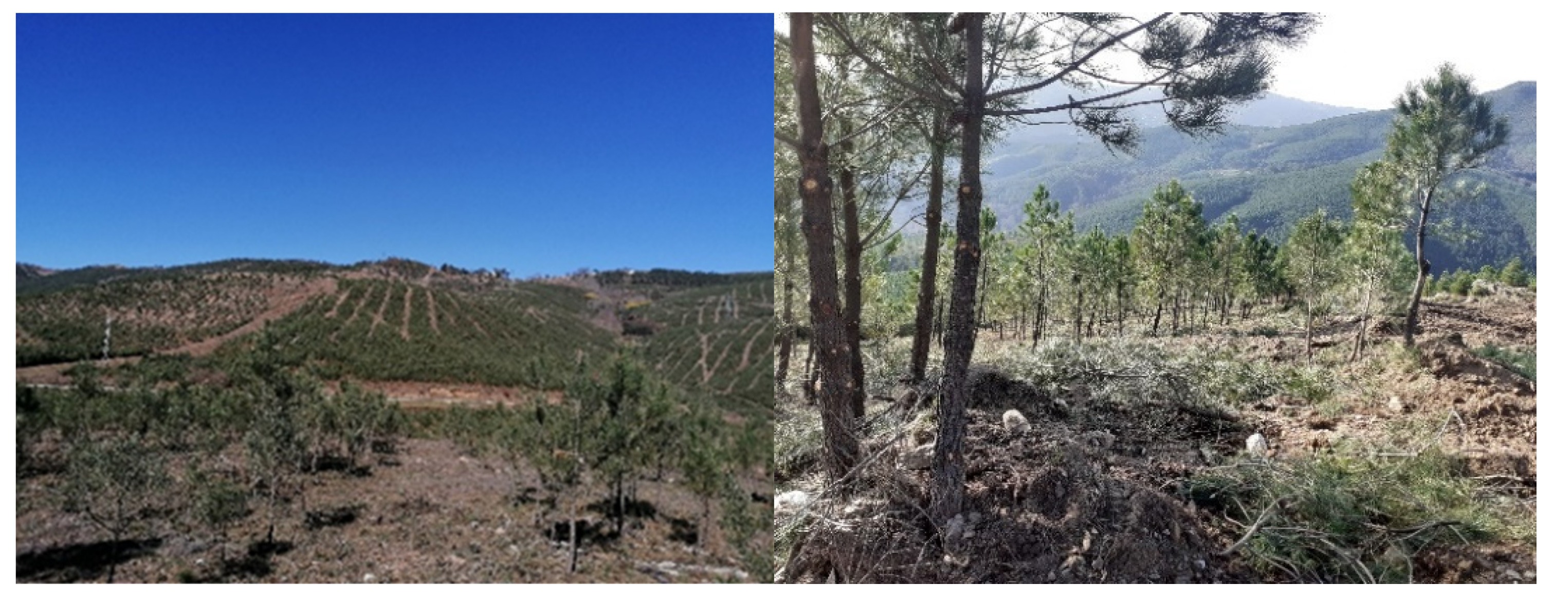
Natural regenerated stands of Pinus pinaster in the study area.

Figure 3.
Forest area of maritime pine by age class in 2021.

Figure 4.
Removed timber volume (m3) by each 5-year period during the planning horizon, T1 = [1,5], T2 = [6,10], T3 = [11,15], T4 = [16,20], T5 = [21,25], T6 = [26,30], with models FMPb (base model), FMPs (model with stability constraints), FMPr (model with revenues per common land constraints), FMPv (model with balanced revenue of volume constraints), FMPy (model with area by classes of age regulation constraints) and FMP (model with all constraints, beyond aforementioned constraints, includes also forest stability constraints and revenues per common land).

Figure 5.
Area (ha) by age class, Y1 = [0,10], Y2 = [11,20], Y3 = [21,30], Y4 = [31,40], Y5 = [41,70], in the last period of the planning horizon according to the results of models FMPb, FMPr, FMPs, FMPv, FMPy and FMP.
Figure 5.
Area (ha) by age class, Y1 = [0,10], Y2 = [11,20], Y3 = [21,30], Y4 = [31,40], Y5 = [41,70], in the last period of the planning horizon according to the results of models FMPb, FMPr, FMPs, FMPv, FMPy and FMP.

Figure 6.
Area (ha) by age class, Y1 = [0,10], Y2 = [11,20], Y3 = [21,30], Y4 = [31,40], Y5 = [41,70], in the last period of the planning horizon according to the results of model FMPs for the whole management (left) and for the independent management (right).
Figure 6.
Area (ha) by age class, Y1 = [0,10], Y2 = [11,20], Y3 = [21,30], Y4 = [31,40], Y5 = [41,70], in the last period of the planning horizon according to the results of model FMPs for the whole management (left) and for the independent management (right).


Table 1.
Major strata identified in the study area based on density and age classes criteria.
| Density/Age | Saplings (0–5 yr) | Young-1 (6–12 yr) | Young-2 (13–20 yr) | Adult-1 (21–30 yr) | Adult-2 (31–40 yr) | Mature (>40 yr) |
|---|---|---|---|---|---|---|
| Low (≤500 trees ha−1) | - | + | + | + | + | + |
| Medium (501–1500 trees ha−1) | + | + | + | + | + | + |
| High (1501–3000 trees ha−1) | + | + | + | + | + | + |
| Very high (3001–10,000 trees ha−1) | + | + | + | + | - | - |
| Extremely high (>10,000 trees ha−1) | - | - | + | + | - | - |
Legend: - combination not found; + combination identified in the study area.
Table 2.
Summary characteristics of the major stand variables evaluated in the 23 study plots.
| Variable | Min | Mean | Max | sd |
|---|---|---|---|---|
| t (yr) | 4 | 22.5 | 65 | 15.4 |
| N (trees ha−1) | 300 | 2736 | 15350 | 3799 |
| G (m2·ha−1) | 0.2 | 17.6 | 42.4 | 10 |
| SI35 (m) | 12.5 | 16.9 | 23.6 | 2.67 |
| dg (cm) | 1.2 | 12.6 | 42.4 | 10.6 |
| ddom (cm) | 1.7 | 18.7 | 46.9 | 12.1 |
| hdom (m) | 1.4 | 10 | 26.3 | 6.5 |
| hg/dg | 42.2 | 88.7 | 337.5 | 60.8 |
| CBD | 0.04 | 0.13 | 0.32 | 0.07 |
Legend: t—stand age (yr); N—number of trees per hectare (trees ha−1); G—basal area per hectare (m2·ha−1); SI35—Site index, defined as the stand dominant height at reference age of 35 years (m); dg—quadratic mean diameter at the height level of 1.30 m (cm); ddom—dominant diameter (cm); hdom—dominant height (m); hg/dg—stability coefficient; CBD—canopy bulk density (km/kgm−3); Min—data minimum; Mean—data average; Max—data maximum; sd—data standard deviation.
Table 3.
Mathematical models’ description.
| Model | Constraints Characterization | Objective Function | Constraints |
|---|---|---|---|
| FMPb |
| (1) | (2)–(6), (16) |
| FMPs |
| (1) | (2)–(7), (16) |
| FMPr |
| (1) | (2)–(6), (8), (9), (16), (17) |
| FMPv |
| (1) | (2)–(6), (10), (11), (16) |
| FMPy |
| (1) | (2)–(6), (12)–(16), (18)–(19) |
| FMP |
| (1) | (2)–(19) |
Table 4.
Used parameters in the models.
| 30 | 16 | 892 | 5 | 8 | 186 | 0.3 | 0.5 |
Legend: nt—number of years in the planning horizon; ns—number of stands; nb—number of common lands constrained to have incomes on period; subset of periods to impose constraints on age class area; tA—target area, in ha, to each class of age; tol—years tolerance to perform a clear-cut; M—big constant; —margin for target removed volume; —margin for target area age class; K—set of age classes.
Table 5.
Mathematical models’ description for individual management.
| Model | Constraints Characterization | Objective Function | Constraints |
|---|---|---|---|
| FMPb-IND |
| (1) | (2)–(6), (16) |
| FMP-IND |
| (1) | (2)–(9), (12)–(14), (16)–(20) |
Table 6.
Model size, branch-and-bound performance, and optimal objective function.
| Model | Model Size | Branch and Bound | Optimal Value (m3 × 103) | ||
|---|---|---|---|---|---|
| # Var | # Constr | Time (s) | Gap (%) | ||
| FMPb | 187,375 | 144,101 | 13.4 | 0.0 | 1928.7 |
| FMPs | 187,375 | 144,683 | 15.9 | 0.0 | 1913.9 |
| FMPr | 187,855 | 145,461 | 14.5 | 0.0 | 1927.9 |
| FMPv | 187,375 | 144,111 | 334 | 0.0 | 1830.4 |
| FMPy | 187,375 | 144,101 | 18.5 | 0.0 | 1680.2 |
| FMP | 187,855 | 146,053 | 1072.3 | 0.0 | 1644.0 |
Legend: # var—number of variables; # constr—number of constraints; time—execution time, in seconds; Gap—the final relative gap, in %; Optimal value—volume removed during all the planning horizon, in 103 m3.
Table 7.
Characterization of FMPb, FMPv, FMPy and FMP according to the optimal value of volume removed over the planning horizon of 30 years, discriminated by clear-cut and thinning.
Table 7.
Characterization of FMPb, FMPv, FMPy and FMP according to the optimal value of volume removed over the planning horizon of 30 years, discriminated by clear-cut and thinning.
| Variable | FMPb | FMPv | FMPy | FMP |
|---|---|---|---|---|
| vol-cc (m3) | 1,031,475.6 | 984,142.5 | 780,566.6 | 751,134.6 |
| vol-th (m3) | 897,223.9 | 846,277.4 | 899,594.0 | 892,822.2 |
| Total vol. (m3) | 1,928,699.5 | 1,830,419.9 | 1,680,160.6 | 1,643,956.8 |
Legend: vol-cc—volume removed in clear-cut, in m3; vol-th—volume removed by thinning, in m3; Total vol.—total volume removed, in m3.
Table 8.
Average age at the end of planning horizon, in the optimal solutions for the six models, FMPb, FMPs, FMPr, FMPv, FMPy and FMP.
Table 8.
Average age at the end of planning horizon, in the optimal solutions for the six models, FMPb, FMPs, FMPr, FMPv, FMPy and FMP.
| FMPb | FMPs | FMPr | FMPv | FMPy | FMP | |
|---|---|---|---|---|---|---|
| 10.96 | 11.45 | 11.01 | 14.59 | 19.94 | 22.28 |
Table 9.
Characterization of FMP and FMP-IND results according to the optimal solution during the planning horizon.
Table 9.
Characterization of FMP and FMP-IND results according to the optimal solution during the planning horizon.
| 5-Years Period | FMP | FMP-IND | ||||||
|---|---|---|---|---|---|---|---|---|
| Cc | Th | Cc | Th | |||||
| n | A (ha) | n | A (ha) | n | A (ha) | n | A (ha) | |
| 20 | 76.8 | 168 | 947.7 | 12 | 53.1 | 171 | 959.0 | |
| 127 | 478.8 | 212 | 1195.9 | 39 | 147.6 | 272 | 1446.8 | |
| 59 | 211.2 | 466 | 2964.4 | 0 | 0.0 | 499 | 3113.1 | |
| 91 | 475.5 | 488 | 3125.2 | 3 | 17.5 | 647 | 3753.2 | |
| 55 | 356.5 | 516 | 3101.0 | 70 | 470.0 | 479 | 2967.9 | |
| 177 | 1147.5 | 244 | 1306.2 | 373 | 2007.7 | 202 | 1072.5 | |
Legend: —first 5-year period (1–5 years); —second 5-year period (6–10 years); —period 11–15 years; —period 16–20 years; —period 21–25 years; —period 26–30 years; n—number of stands; A—area, in ha; Cc—clear-cut; Th—thinning.
Table 10.
Characterization of the base and complete optimization models, by management type, in the optimal solutions achieved for a set of 18 common lands, in terms of total volume removed (Vol., m3) and average age (, yr) at the end of the planning period.
Table 10.
Characterization of the base and complete optimization models, by management type, in the optimal solutions achieved for a set of 18 common lands, in terms of total volume removed (Vol., m3) and average age (, yr) at the end of the planning period.
| Global Joint Management (G) | Independent Management (I) | 100(G-I)/G | |||||
|---|---|---|---|---|---|---|---|
| Model | Vol. (m3) | Model | Vol. (m3) | Vol. | |||
| FMPb | 1,901,081.9 | 10.09 | FMPb-IND | 1,905,323.9 | 10.04 | −0.22 | +0.50 |
| FMP | 1,626,701.4 | 21.00 | FMP-IND | 1,766,397 | 20.44 | −8.59 | +2.67 |
Publisher’s Note: MDPI stays neutral with regard to jurisdictional claims in published maps and institutional affiliations. |
© 2022 by the authors. Licensee MDPI, Basel, Switzerland. This article is an open access article distributed under the terms and conditions of the Creative Commons Attribution (CC BY) license (https://creativecommons.org/licenses/by/4.0/).
Share and Cite
MDPI and ACS Style
Cabral, M.; Fonseca, T.F.; Cerveira, A. Optimization of Forest Management in Large Areas Arising from Grouping of Several Management Bodies: An Application in Northern Portugal. Forests 2022, 13, 471. https://doi.org/10.3390/f13030471
AMA Style
Cabral M, Fonseca TF, Cerveira A. Optimization of Forest Management in Large Areas Arising from Grouping of Several Management Bodies: An Application in Northern Portugal. Forests. 2022; 13(3):471. https://doi.org/10.3390/f13030471
Chicago/Turabian StyleCabral, Margarida, Teresa Fidalgo Fonseca, and Adelaide Cerveira. 2022. "Optimization of Forest Management in Large Areas Arising from Grouping of Several Management Bodies: An Application in Northern Portugal" Forests 13, no. 3: 471. https://doi.org/10.3390/f13030471
Note that from the first issue of 2016, this journal uses article numbers instead of page numbers. See further details here.