
Estimating Aboveground Biomass in Dense Hyrcanian Forests by the Use of Sentinel-2 Data
by
 , , and
Fardin Moradi
1,* ,
,
Ali Asghar Darvishsefat
1 ,
,
Manizheh Rajab Pourrahmati
1,
Azade Deljouei
2 and
Stelian Alexandru Borz
2,* 1
Department of Forestry and Forest Economics, Faculty of Natural Resources, University of Tehran, Karaj P.O. Box 1417643184, Iran
2
Department of Forest Engineering, Forest Management Planning and Terrestrial Measurements, Faculty of Silviculture and Forest Engineering, Transilvania University of Brasov, Şirul Beethoven 1, 500123 Brasov, Romania
*
Authors to whom correspondence should be addressed.
Forests 2022, 13(1), 104; https://doi.org/10.3390/f13010104
Submission received: 13 December 2021
/
Revised: 6 January 2022
/
Accepted: 10 January 2022
/
Published: 12 January 2022
(This article belongs to the Special Issue Electronics, Close-Range Sensors and Artificial Intelligence in Forestry)
Abstract
:Due to the challenges brought by field measurements to estimate the aboveground biomass (AGB), such as the remote locations and difficulties in walking in these areas, more accurate and cost-effective methods are required, by the use of remote sensing. In this study, Sentinel-2 data were used for estimating the AGB in pure stands of Carpinus betulus (L., common hornbeam) located in the Hyrcanian forests, northern Iran. For this purpose, the diameter at breast height (DBH) of all trees thicker than 7.5 cm was measured in 55 square plots (45 × 45 m). In situ AGB was estimated using a local volume table and the specific density of wood. To estimate the AGB from remotely sensed data, parametric and nonparametric methods, including Multiple Regression (MR), Artificial Neural Network (ANN), k-Nearest Neighbor (kNN), and Random Forest (RF), were applied to a single image of the Sentinel-2, having as a reference the estimations produced by in situ measurements and their corresponding spectral values of the original spectral (B2, B3, B4, B5, B6, B7, B8, B8a, B11, and B12) and derived synthetic (IPVI, IRECI, GEMI, GNDVI, NDVI, DVI, PSSRA, and RVI) bands. Band 6 located in the red-edge region (0.740 nm) showed the highest correlation with AGB (r = −0.723). A comparison of the machine learning methods indicated that the ANN algorithm returned the best ABG-estimating performance (%RMSE = 19.9). This study demonstrates that simple vegetation indices extracted from Sentinel-2 multispectral imagery can provide good results in the AGB estimation of C. betulus trees of the Hyrcanian forests. The approach used in this study may be extended to similar areas located in temperate forests.
1. Introduction
Forests are an essential component of the carbon cycle, as they are both storing and releasing carbon through their biomass into the atmosphere. Globally, forest ecosystems contain approximately 80% of the aboveground and 40% of the underground biomass [1]. Knowledge on the amount of biomass and carbon storage is essential for forest management and planning [2]. Quantifying biomass availability in the forests through field measurements is commonly resource-intensive. Remote sensing techniques integrated with geographic information systems (GISs) provide quick access to useful information, typically available for short cycle times and at lower costs [3]. Combining remotely sensed data with nonspectral ancillary data such as those produced by field sampling has been suggested by many studies as a way to reach better estimates [4]. A variety of remotely sensed data, such as those coming from Landsat, Sentinel, Spot, and ALOS missions, have been used to estimate the volume of wood and biomass stocked in the forests [5,6,7,8,9,10,11,12,13].
Aboveground biomass (AGB) estimation methods include field measurements and remote sensing approaches [14,15]. There are mainly two methods used in field measurement to estimate the AGB, namely destructive (harvesting) and nondestructive methods. Although the destructive method is useful and accurate in developing equations for the assessment of aboveground biomass over larger areas, it is often constrained to few trees, being time consuming, difficult to implement, and expensive [16]. A nondestructive method is an alternative to estimate the AGB. It is implemented either by climbing to make measurements in different tree parts or, more commonly, by measuring the diameter at the breast height (DBH) and tree height; other options include the estimation of volume and density using allometric equations or remote imagery [17,18]. As a nondestructive method, remote sensing is based on previously developed allometric equations.
The techniques used for estimating the AGB of forests based on remotely sensed data can be divided into two categories, namely those using parametric (statistical regression methods) and nonparametric algorithms, respectively [7]. Nonparametric techniques, including Machine Learning (ML) algorithms such as the k-Nearest Neighbor (kNN), Artificial Neural Networks (ANNs), and Random Forests (RFs), were found to hold a better ability of identifying complex relations between the used predictors and the AGB [7,19]. For instance, ANNs are being considered to be important nonparametric algorithms for estimating forest-related parameters [20]. In addition, the kNN algorithm has received considerable attention because it is easily accessible, and some literature reviews have shown that it holds an excellent capability to increase the precision when estimating vegetation parameters [21,22,23]. RF regression algorithms have also been widely used for quantifying forest biophysical parameters [5,24,25,26], standing for an ensemble learning algorithm with applications in classification and regression problems. The RF algorithm was developed by Breiman [27] and can be used to predict continuous and categorical dependent variables. A random subset of observations with replacement, as well as a random set of explanatory variables, are used to build each regression tree [28].
Traditionally, in any part of the world, AGB is estimated by destructive methods, which are used to develop allometric equations based on measured parameters collected from harvested trees (e.g., DBH, tree height, and timber volume) [29]. However, applying allometric equations across a large study area is cumbersome and sometimes impractical as the field measurement input parameters are rare and sometimes unavailable. In comparison, remote sensing techniques can provide large-scale and accurate biophysical information for forest inventory data. Hence, remote sensing data combined with machine learning techniques (i.e., parametric and nonparametric algorithms) have been widely used to estimate forest AGB in the past decade. For example, Muukkonen and Heiskanen [30] predicted the AGB in boreal forests using ANNs applied to ASTER (Advanced Spaceborne Thermal Emission and Reflection Radiometer) data. IRS P6 LISS-III (Indian Remote-Sensing Satellite-P6 Linear Imaging Self-Scanning Sensor-3) data were used by Yadav et al. [31] to estimate the AGB in the Timli forests of India. In their research, the kNN method based on Mahalanobis distance outputted a RMSE of 42.25 Mg/ha, while the distance metric used was found to be best, being followed by the fuzzy and Euclidean distances, with RMSE of 44.23 Mg/ha and 45.13 Mg/ha, respectively. Lu et al. [32] showed that the estimation of AGB in Amazon forests using Landsat-5 TM data is more accurate in young than in mature stands. Ronoud et al. [33] found that the Landsat-5 TM NIR (near-infrared) band exhibited the highest correlation with AGB (r = 0.427). Several studies have used Sentinel-2 data to estimate AGB in various ecosystems, including semiarid [34], Mediterranean [35,36], temperate [7,37,38], tropical [37,39,40], subtropical [41,42] and boreal [43,44] forests, and grasslands [45]. For example, Chrysafis et al. [46] compared Sentinel-2 MSI (MultiSpectral Instrument) and Landsat-8 OLI (Operational Land Imager) imagery for forest growing stock volume (GSV) estimation in a mixed Mediterranean forest in northeastern Greece. GSV was modeled using RF regression based on spectral bands and vegetation indices. They have shown that to estimate the AGB, Sentinel-2 data with an R2 = 0.63 and RMSE = 63.11 m3/ha were better than Landsat-8 OLI data with an R2 = 0.62 and RMSE = 64.40 m3/ha. According to Castillo et al. [37], red and red edge bands produced by Sentinel-2 data combined with elevation data provided the best estimates of AGB in Philippine’s mangrove forests when using machine learning methods. Nuthammachot et al. [47] assessed the potential of seven vegetation indices derived from Sentinel-2 images for estimating the AGB in a private forest of Indonesia. They found that, among other indices, including the Normalized Difference Vegetation Index (NDVI), Enhanced Vegetation Index (EVI), Modified Simple Ratio (MSR), Simple Ratio (SR), Sentinel-2 Red-Edge Position (S2REP), and Greenness Normalized Difference Vegetation Index (GNDVI), the Normalized Difference Index (NDI45) exhibited the strongest correlation with AGB (r = 0.89, R2 = 0.79). In addition, they found that the NIR spectral band of the Sentinel-2 was the most effective variable in retrieving forest standing volume when using the kNN algorithm. They estimated the standing volume with a relative RMSE of 22.94%. Research by Pandit et al. [42] evaluated the usefulness of Sentinel-2 data for estimating the AGB in protected forests from Nepal using the RF algorithm. The effect of the number of input variables, including spectral band values and spectral-derived vegetation indices on the AGB prediction, was also investigated. The model using all spectral bands, in addition to the derived vegetation indices, provided better AGB estimates (R2 = 0.81 and RMSE = 25.57 t/ha). Vafaei et al. [48] assessed ALOS-2 (Advanced Land Observing Satellite 2) and Sentinel-2 data for AGB estimation in the Asalem forests of Iran using four machine learning methods, namely the Gaussian process (GP), support vector regression (SVR), RF, and Multi-Layer Perceptron Neural Networks (MLP Neural Nets, MLP NNs). In their study, a SVR model using combined Sentinel-2 spectral information (including blue, green, red, and NIR bands) and six vegetation indices, namely SVI (Simple Vegetation Index), RVI (Ratio Vegetation Index), NDVI (Normalized Difference Vegetation Index), EVI-2 (Enhanced Vegetation Index 2), PVI-2 (Perpendicular Vegetation Index 2), and SAVI (Soil Adjusted Vegetation Index) based on ALOS-2 PALSAR2 (Advanced Land Observing Satellite 2, Phased-Array-type L-band Synthetic Aperture Radar 2) imagery, HH (horizontal transmit and horizontal receive), HV (horizontal transmit and vertical receive), VV (vertical transmit and vertical receive), and VH (vertical and horizontal receive), yielded the best performance to estimate the forest AGB.
Data saturation often causes problems in estimating forest AGB when dealing with high amounts of biomass or high-canopy-density areas [49]. This problem was addressed by combining Sentinel-2 and ALOS2-PALSAR2 data [48]. The studies mentioned above, which evaluated the utility of remotely sensed data for estimating the forest standing volume and AGB, do not show consistency in performance and outcomes, due to the variety of forest conditions, satellite data used, applied methodology, and due to the inherent, specific limitations of each study.
In Iran, an area of ~10.7 million hectares is covered by forests accounting for ca. 7.4% of the country’s territory [50]. Hyrcanian forests are the most important forests among the five vegetation regions in Iran due to the density, canopy cover, and diversity in this ecoregion [51,52]. They cover ~2 million hectares and are located on the south coast of the Caspian sea [53]. For these forests, management plans are updated in terms of qualitative and quantitative attributes every ten years, in which collecting data and information are time-consuming and cost-intensive. In contrast, remotely sensed imagery holds a promising potential for monitoring and continuously predicting forest attributes. In conjunction with satellite data, field data can be used to create a continuous map of forest attributes through classification or regression. Therefore, forest attributes have been estimated from remote sensing data with various spatial resolutions, ranging from very high to medium.
To the best of our knowledge, this is the first study attempting to estimate the AGB by the use of remotely sensed data and machine learning algorithms in pure common hornbeam (Carpinus betulus L.) forests, as a typical forest type in the temperate forest region of many European and Asian countries. This study was guided by the above mentioned, as well as the fact that pure stands of common hornbeam are distributed from 200 to 1800 m a.s.l., from the western part, characterized by a very humid climate, to the eastern part of the Hyrcanian region, which is characterized by a humid climate [54]. Accordingly, this study aimed to evaluate the usefulness of Sentinel-2 imagery and several machine learning algorithms for estimating the AGB of C. betulus forests located in the Patom and Namkhane districts of Kheyrud forest, Northern Iran. The objectives of the study were the following: (i) comparing the performance of different AGB estimation approaches including parametric (i.e., Multiple Regression—MR) and nonparametric algorithms (ANN, kNN, and RF), and (ii) investigating the potential and capability of Sentinel-2 imagery in improving the accuracy of the AGB estimation under the given conditions of the study.
2. Materials and Methods
2.1. Study Site
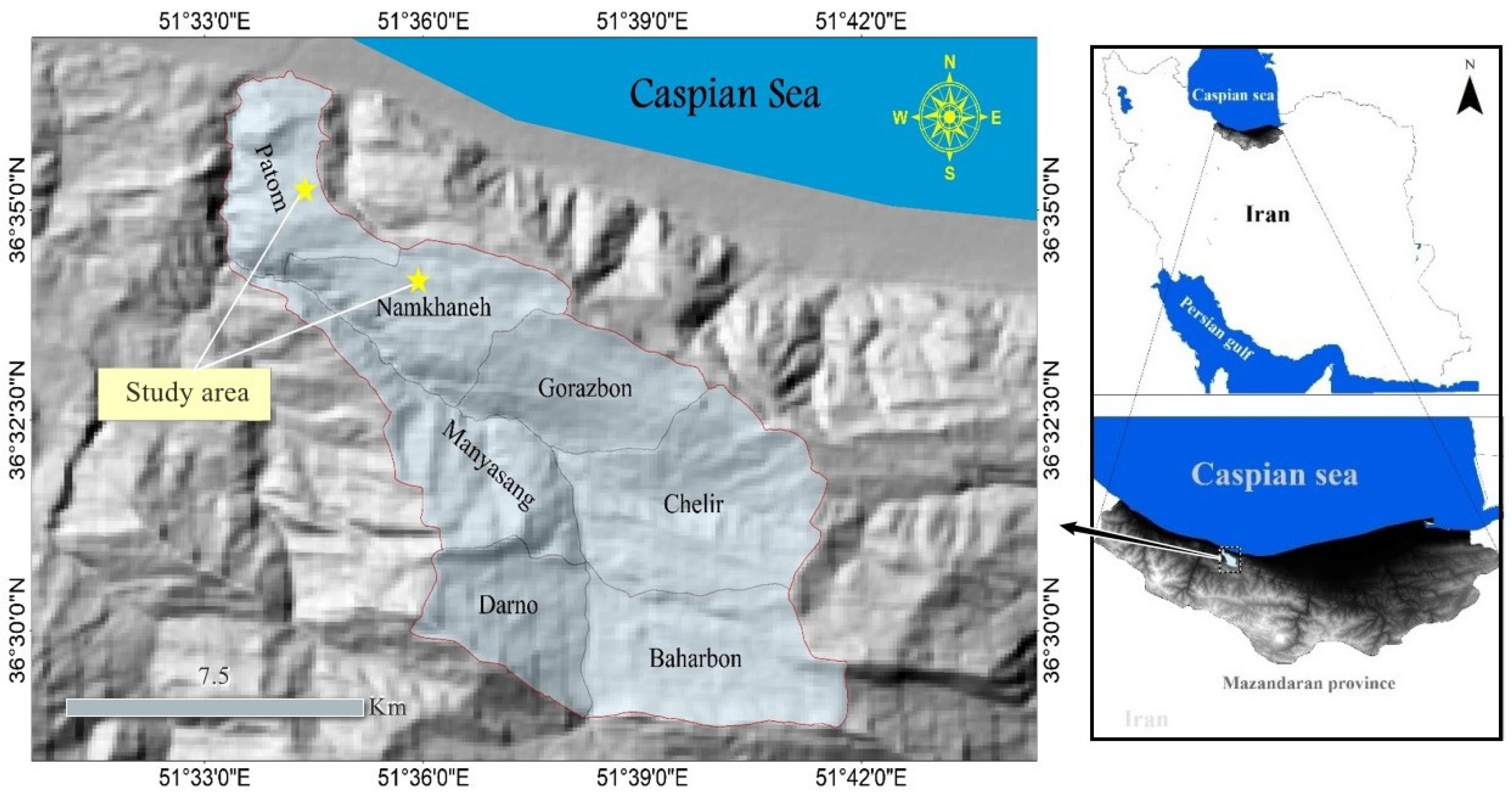
The study area is located in the Kheyrud forest as part of the mountainous deciduous forests of the Hyrcanian ecoregion, north of Iran (longitude: 51°34′53″ to 51°35′28″ E and latitude: 36°36′14″ to 36°35′28″ N). Kheyrud forest covers a total area of ~8000 ha, and it is a natural and mature forest with uneven-aged and dense to semi-dense stands consisting of seven management districts. Two study sites were selected in Patom and Namkhane districts (Figure 1). The elevation of the selected areas ranges from 480 to 630 m a.s.l. in Patom and from 950 to 1110 m a.s.l. in Namkhane district. According to the Nowshahr synoptic station [51,55], the climate of the area is sub-Mediterranean with an annual temperature averaging 9 °C and a total annual precipitation of 1300 mm. Tilio-buxetum, Querco-carpinetum, Fageto-carpinetum, and Rusco-Fagetum are the main forest communities in the Patom district. Namkhane district contains forest communities of Querco-carpinetum, Fageto-carpinetum, Fagetum mixed, and Fagetum-hyrcanum [34]. Sample plots were selected on flat areas, in pure stands of C. betulus to minimize the spectral interference of other species [56]. The stock of C. betulus stands based on our plot-level measurements ranged from 174 to 470 m3 ha−1.
2.2. Remote Sensed Data and Data Preprocessing
Sentinel-2 satellite data (dated 17 July 2016) were obtained from the US Geological Survey (USGS) website (https://earthexplorer.usgs.gov/; accessed on 25 March 2017) and used for AGB estimation. Sentinel-2 carries the Multispectral Imager (MSI) that delivers 13 spectral bands with a spatial resolution ranging from 10 to 60 m. Sentinel-2 10 m spatial resolution bands including B2 (490 nm), B3 (560 nm), B4 (665 nm), and B8 (842 nm), and 20 m spatial resolution bands of B5 (705 nm), B6 (740 nm), B7 (783 nm), B8a (865 nm), B11 (1610 nm), and B12 (2190 nm) were used for analysis. The three 60 m bands (bands 1, 9, and 10), which are mainly focused toward cloud screening and atmospheric correction [57], have not been taken into consideration in this study. The digital topographic maps available at a scale of 1:25,000 and provided by the National Cartographic Center (NCC) of Iran were used to evaluate the geometric accuracy of the satellite image, which was evaluated based on road features extracted from topographic maps.
The sixth version of the Sentinel Application Platform (SNAP) software developed by the European Space Agency (ESA) was used to process the Sentinel-2 data. A visual assessment of radiometric quality was also performed concerning the presence of cloud cover, a scanning line, and duplicated pixels. Then, the two well-known processing methods, namely Principal Component Analysis (PCA) and the spectral band ratio, were applied to all original spectral bands of the images. Table 1 describes the vegetation indices extracted using band rationing.
2.3. In Situ Measurements
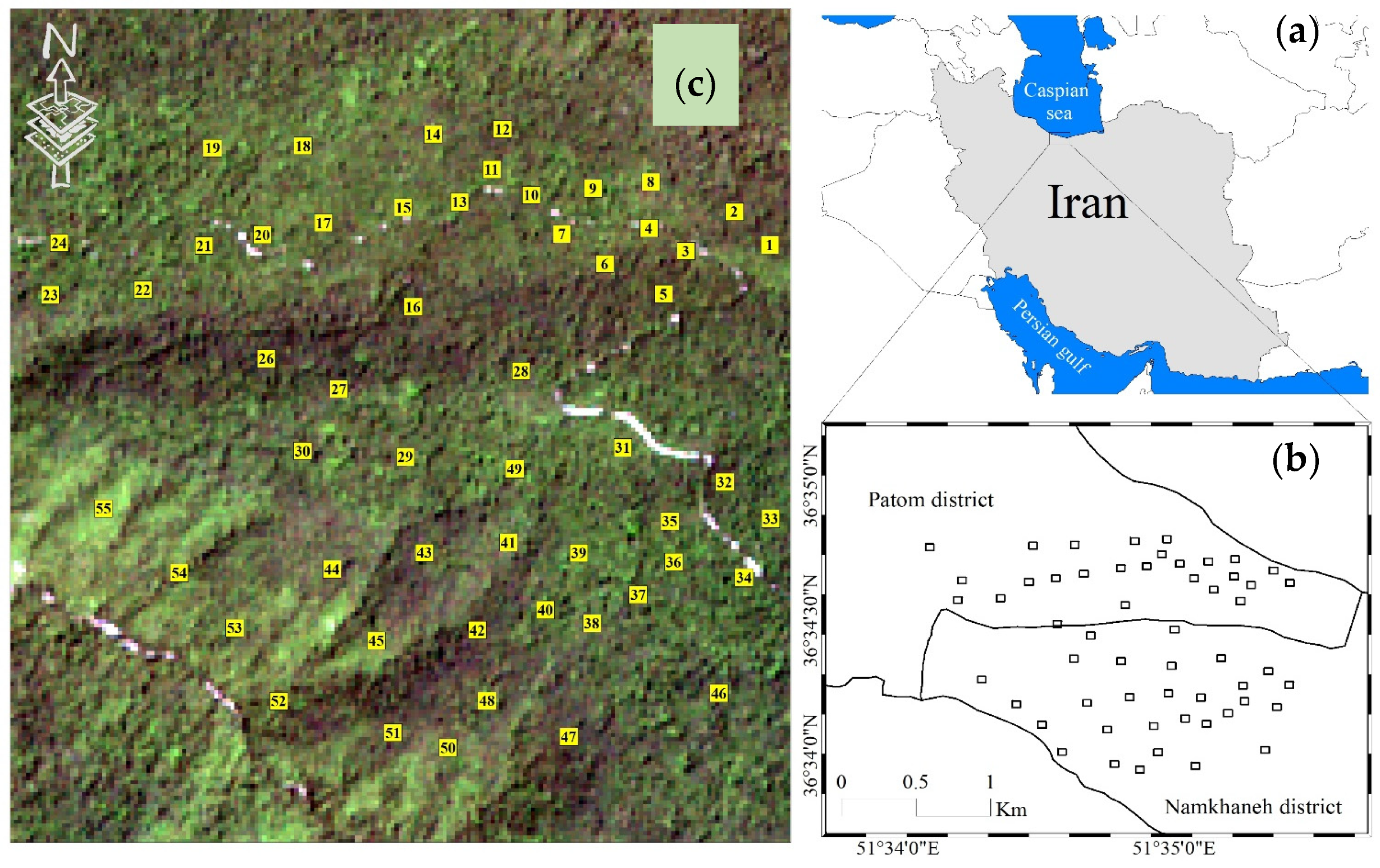
Field measurements were conducted to estimate the AGB in August 2016, and in situ data were collected over 55 plots (45 × 45 m; Figure A1) that were navigated by GPS (Garmin Colorado 300; Olathe, KS, USA). Sample plots were distributed selectively to meet the homogeneity of plots in terms of species, terrain slope, and aspect due to the diverse topographic conditions and small extent of pure C. betulus stands over the study sites. The DBHs of all trees having a diameter greater than 7.5 cm and species were recorded for each plot. The volume of individual trees was estimated using a local tarif volume table and aggregated at the plot level. Then, AGB (t/ha) was estimated for each plot using Equation (1) [66].
where Volume is the volume per hectare derived from the local tariff table, and WD (t/m3) is the wood density. The value of 0.68 t/m3 was used for C. betulus as a WD [67].
2.4. Methods
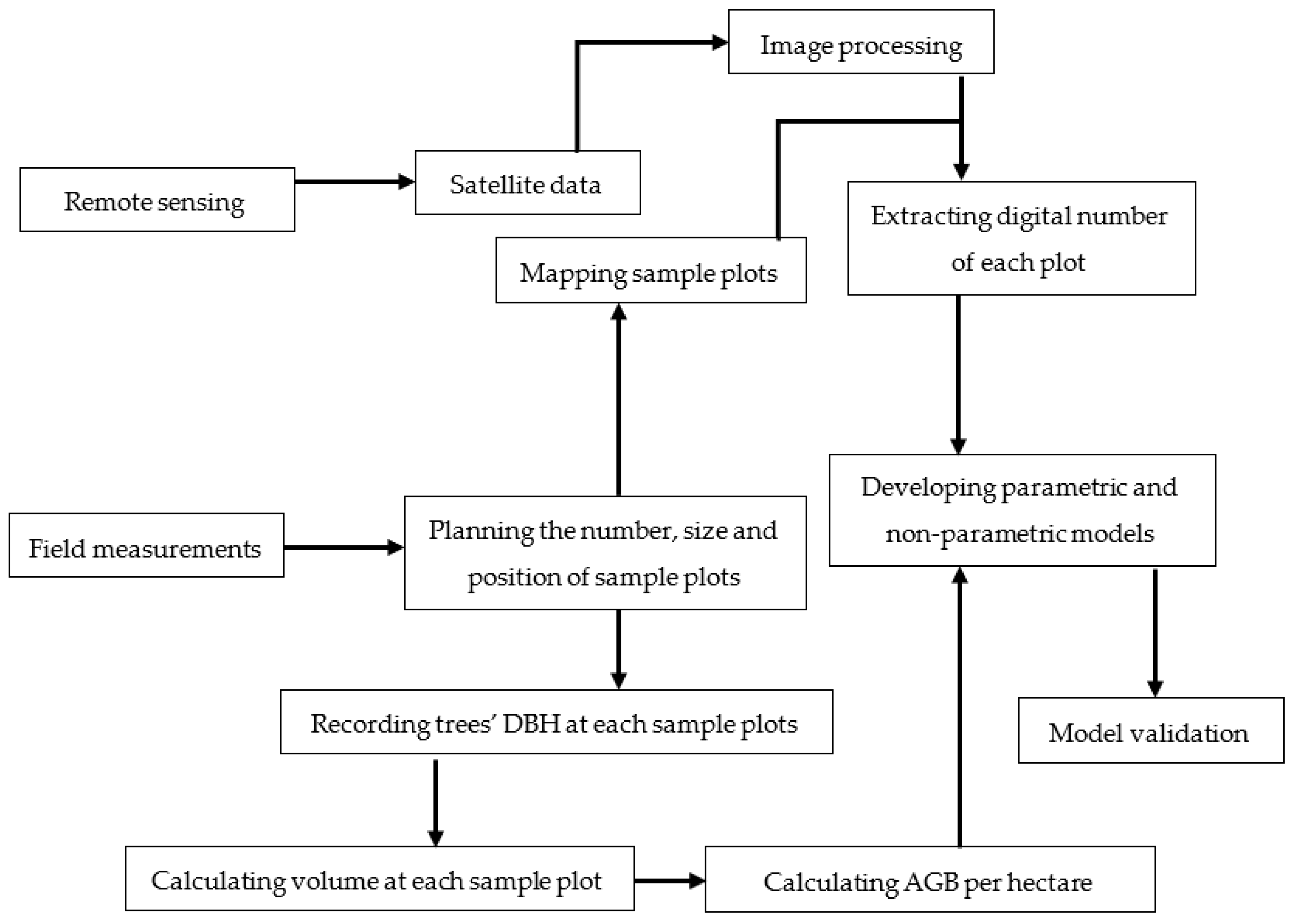
The flowchart of AGB estimation is shown in Figure 2. Pearson’s correlation was used to describe the association between AGB and the corresponding spectral values. The AGB (dependent variable) was modeled based on the remote sensing metrics (independent variables) using the parametric method of MR, as well as the well-known nonparametric algorithms of ANNs, kNN [68], and RF [28]. In the MR method, the model was fitted using all variables (main and synthetic spectral imagery). The suitable remote sensing variables that had a strong correlation with AGB were identified by the means of backward elimination and stepwise selection procedures [69]. Before implementing the MR, the normality of the dataset was evaluated using the Kolmogorov—Smirnov test [70].
Typically, the ANN contains a large number of interconnected nodes and uses mathematical algorithms to model nonlinear problems such as modeling the forest biomass. The MLP (MultiLayer Perceptron) NN model is one of the most commonly used neural network algorithms for environmental modeling, monitoring, mapping of forests, and estimating the forest biomass [69,71,72]. The typical architecture of the MLP NN consists of at least three layers and includes the input, hidden, and output layers. Each layer is composed of several nodes or neurons. The number of neurons used in the input layer was that of the number of input explanatory variables. A significant influence on the performance of the MLP NN model is given by the connection weights between the input and hidden layers, as well as the connection weights between the hidden and output layers. Nonetheless, there is no rule that allows previous decisions to determine the number of neurons in the hidden layer or the number of hidden layers. Some have reported that an insufficient number of hidden neurons made the network learning difficult [73], whereas an excessive number of hidden neurons might lead to unnecessary training time [74]. Therefore, the commonly used strategy to reach the optimum number of neurons in the hidden layer is by trial and error [75]. The output layer contained one neuron and was used to output estimated values of the AGB. The weights assigned at the connections between the input, hidden, and output layers were updated in the training phase and were based on a back-propagation algorithm [76] that minimized the differences between the AGB value estimated by the MLP NN and that produced from AGB in situ inventories. The process was repeated until reaching a predefined accuracy level or the maximum number of iterations.
To develop the architecture of the MLP NN model, in this study, the number of selected hidden neurons was significantly impacting the estimation of AGB [72], as defined by [77]. As a result, by varying the number of neurons against the root-mean-square error (RMSE) based on the data contained in the training dataset, the best MLP NN models were reached. These best models were described by the highest R2 and the lowest RMSE. Accordingly, the best MLP NN model was found to be that characterized by two hidden layers containing four neurons in the first and two neurons in the second layer. The model was trained using 70% of the dataset, and the remaining data (30%) were split in half for validation (15%) and testing (15%). The steps described above were implemented in the Statistica software (Ver. 10).
For the kNN algorithm, the choice of the k value, distance metric, and weighting function are critical factors affecting the estimation accuracy [32]. The model performance was tested by the use of k values from 1 to 40 to find the optimum one for implementing the kNN algorithm [23,78]. Moreover, for an efficient comparison of the distance metrics in the kNN implementation, the four distance metrics available in Statistica software (StatSoft. Inc., Tulsa, OK, USA), including the Euclidean, squared Euclidean, Manhattan (city block), and Chebychev distances (Equations (2)–(5)), were used, and their results were compared against each other [78].
The most frequently used distance metric is the Euclidean distance, standing for a simple geometric distance in a multidimensional space [79]. In the case of squared Euclidean distance, the distance between the target and reference units would be squared to give progressively greater weights to data points that are closer or more similar. Absolute distances are considered when using the Manhattan distance metric, although the effect of single large differences (i.e., outlier data) is dampened whether they are not squared [79]. The absolute magnitude of differences between coordinates of a pair of data points was examined by Chebychev’s distance metric. This metric can be used for both ordinal and quantitative variables and it is appropriated when one would like to term two data points as “different” if they are different on any one of their dimensions.
where D is the distance between the target and reference units, x is the target unit, and p is the reference unit in all equations. The squared Euclidean distance is the most commonly used distance metric among the four mentioned above [78,80,81,82].
RF is an efficient machine learning algorithm that was developed by Breiman [28], currently being used for classification and regression problems. Typically, its use yields high accuracy, being robust in finding outliers and noise, computes quickly, and shows the relative importance of the input variables [83]. A bagging algorithm [84] is used to generate n sub-datasets (which is called a bootstrap dataset) from the training dataset. By the Classification And Regression Tree (CART) algorithm, each bootstrap dataset is used to construct a base-decision tree [85]. Finally, the RF model is generated by grouping base-decision trees to form a forest. Two-thirds of the total samples from the training dataset, called “in bag” data, should be contained in these bootstrap datasets. Approximately one-third of observations (out-of-bag, OOB) are used to evaluate the RF model [86]. The number of base-decision trees should be selected carefully because the RF model’s performance depends on this parameter. In this study, 500 base-decision trees were selected to ensure the stability of the RF model’s results, as suggested by Stevens et al. [87], and they were used to produce a graph showing the average squared error rates against each number of trees for training and testing samples, as a robust analytical tool to explore data and to verify the optimal number of trees within RFs. In such graphs, the optimal number of trees is determined based on the number of trees that produces a stable error [55]. Following this, we repeated the RF implementation using this optimal number of trees and other fixed parameters.
2.5. Statistical Analysis and Modeling Performance
PCA analysis was used in this study to identify the main components and to help analyze a subset of features by a dimensionality reduction. PCA is widely used to eliminate waste data in remote sensing studies [88]. In this study, PCA was computed from the bands of the Sentinel-2 image, and it was used for AGB modeling by the means of Statistica (version 10) software. The first component of all bands, except band 10, was included in the PCA analysis. In addition, a sensitivity analysis was used to determine the most effective model parameters [89].
Model testing and validation was performed by using 30% of all observations. The estimated performance metrics of the models were developed in the form of statistics such as the root-mean-square error (RMSE), relative RMSE (%RMSE), which were also used to choose the best model, adjusted coefficient of determination (R2adj), and standard error of estimates (SEE). R2adj and SEE were calculated only for regression models, while RMSE and relative RSME were used to evaluate the performance of both parametric and nonparametric models (Equations (6)–(9)).
where AGB and AGBi stand for the estimated and observed AGB per plot, respectively, n is the total number of samples, is the average of the testing phase data, R2 is the coefficient of determination, N is the number of samples, p is the number of predictor variables, and σ is the standard deviation.
3. Results
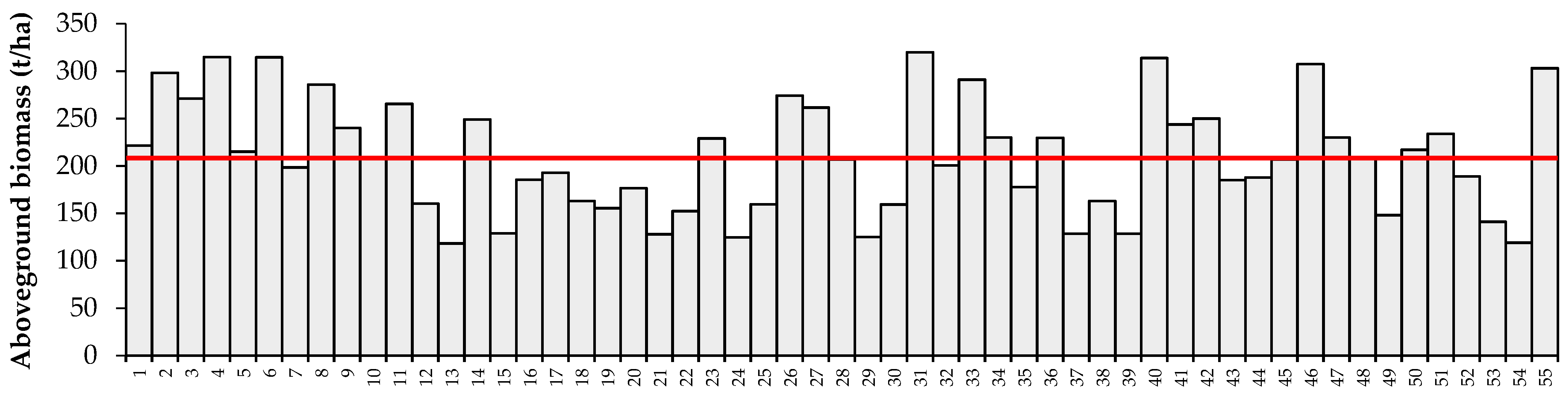
Based on the in situ measurements, the minimum, maximum, and mean values of the AGB for C. betulus stands were estimated at 118, 320, and 210 t/ha, respectively, with a standard deviation of 60 t/ha (Figure 3; Table A1); there was a high variance (3588 t/ha), indicating that the data were spread out from the mean, and from one another (Table A1). The results of the normality test indicated a normal distribution of both in situ and remotely sensed data. Based on Pearson’s correlation coefficient, a negative association was found between spectral information and in situ AGB (Table 2). Band 6 of the Sentinel-2 data outputted the highest correlation with in situ AGB (r = −0.723; Table 2).
The result of the AGB prediction using MR indicated that the backward elimination procedure (R2adj = 0.65, %RMSE = 24.72) outperformed the linear regression that used all the variables, as well as the stepwise regression model (Table 3).
Table 4 shows the performance of the kNN models that included all the variables and used four distance metrics (Euclidean, Squared Euclidean, Manhattan, and Chebychev). The best distance metric for the kNN algorithm was the Manhattan distance, which returned the lowest %RMSE and the highest R2 (Table 4).
The ANN fitted by a MLP NN model with an input layer containing all variables and two hidden layers produced a relative RMSE of 19.93% during the validation phase (Table 5). The sensitivity analysis indicated that PC1 was the most effective variable for estimating AGB.
As mentioned before, the performance of the RF algorithm depends on choosing the optimal number of trees and numbers of predictors (k) in each node for producing a good response in estimations. For instance, Figure 4 shows the average squared error rates against the number of trees used for AGB estimation when using RF during the training and testing phases. The optimal number of trees is assigned to the point where the error rate does not change by increasing the number of trees (Figure 4). The improvement in accuracy was slow after about 220 trees; therefore, this number was used as a good estimation for an optimum number to use (Figure 4). Based on the variable importance value obtained from the sensitivity analysis, spectral band 6 of Sentinel-2 was the most effective variable. In this study, the best RF model estimated AGB with a relative RMSE of 22.55% for k set at 6 (Table 5).
4. Discussion
Previous studies have found that remote sensing-based models for AGB estimation are more accurate than empirical-based and GIS-based models [32]. In this study, Sentinel-2 data were used to estimate the AGB in pure stands of C. betulus in a part of the Hyrcanian forest, Iran. A total of 19 variables, including original spectral bands, vegetation indices, and the first principal component of PCA (applied to all original bands), were used for estimation. In situ AGB was found to be negatively correlated with all variables. The highest correlation was between the AGB and the two spectral bands located at the red edge (0.731–0.749 nm wavelength) and shortwave infrared (1.539–1.681 nm wavelength), with values of R2 of −0.723 and −0.716, respectively. The negative correlation between biomass and spectral values has been discussed in many studies [9,10,11,90], expected to be caused by the canopy shadowing of trees, canopy size, stand volume and density, and consequently, by a more complex vertical structure of the forests. Shadowing is a factor influencing the reduction in spectral reflectance of forests [91]. In addition, the fraction of vegetation cover (FVC) of the ground at the pixel level is another reason affecting the radiation behavior at the canopy level, particularly in taller stands [92,93], which was the case of forests from this study.
The higher spectral radiances of low-density forests characterized by less biomass can be partially explained by a smaller amount of shadows resulting in a higher contribution of the soil to the spectral radiance [12,91]. The age of the studied stands could be another reason for the negative correlation between the amount of AGB and their corresponding spectral values [13,94]. At higher ages, which was the case of this study, the size of the canopy is rising [95], which increases the canopy surface area, size, and number of holes in the canopy [8,94]. Increasing the canopy surface area can reduce the amount of reflection due to the holes created in the tree crowns that is causing the electromagnetic waves to spread through the crown and reduces reflection [94]. In addition, as the age of the trees increases, their requirements for water will increase. As the amount of water increases in the leaves, it will absorb electromagnetic waves and will thus reduce reflection. Furthermore, as the age of the forest stands increases, the number of stories usually develops, causing more propagation of the electromagnetic waves and ultimately a reduction in spectral reflection [10,96]. On the other hand, a positive correlation between biomass and spectral reflectance was reported by different researchers [33,47] and explained by specific characteristics of the study site such as the vertical structure of forest stands, canopy cover percentage, forest health and vitality, species composition, and soil properties. In this study, we found that the relatively strong correlation between AGB and B6, though negative, preserved the presence of this variable in the backward and stepwise regression models (Table 3).
Our results indicated that nonparametric models performed better than MR, and the best result was obtained when using an ANN that outputted a relative RMSE of 19.93%. This is in agreement with the findings of Vafaei et al. [48] (relative RMSE = 19.17%) and close to those of Gao et al. [19] (relative RMSE = 28.8%). The ability to learn during training and to generalize on new datasets makes ANN more powerful and flexible than MR [7,97]. Past research has suggested that whenever an insufficient number of sample plots is available, parametric models can result in a poor performance, while nonparametric models may lead to more accurate predictions [98]. The ANN, as a nonparametric mathematical model, is conceptually similar to biological neural networks and holds excellent linear and nonlinear fitting capabilities [7]. Nevertheless, this is mainly due to the fact that the nonparametric models are able to handle nonlinear relations between variables from multiple sources [34]. By comparing the performance of algorithms for forest AGB estimation on ALOS PALSAR and Landsat data, Gao et al. [19] concluded that ANN performed better than RF. For the temperate forest of China, Chen et al. [7] concluded that ANN was most accurate in assessing the biomass of broadleaved deciduous forests as opposed to regression, SVR, and RF algorithms. As shown by this study, the higher performance of nonparametric algorithms could be due to the complex relations established between AGB and remote sensing variables, which are difficult to understand and explain by parametric algorithms. In addition, nonparametric algorithms are more flexible, by removing some limitations such as the hypotheses on data distribution and the functional form of the mathematical relation between independent and dependent variables. For instance, Lu et al. [32] believed that nonparametric algorithms are more adapted in creating complicated nonlinear biomass models because they do not explicitly predefine the model structure but determine it in a data-driven manner.
As in many other studies, addressing data uncertainty is important. In this study, data uncertainty may be associated with the GPS errors in locating the sample plots, possible errors of the local volume table, the inappropriateness of the available allometric models to calculate the AGB, and spectral interference of other species that existed in the plots. In addition, optical data produced by the Sentinel-2 mission cannot penetrate the forest canopy, preventing it from capturing information about wooden understories. On the one hand, extending the canopy surface will increase the size and number of holes in the canopy. Tree growth will increase in terms of volume, so trees will make a shadow that will cause a reduction in reflection [99]. On the other hand, spreading water on the leaves and increasing the water availability will also reduce the reflectance [99].
Many studies have indicated that integrating multisensor information from optical, radar, and lidar platforms can improve biomass estimation accuracy [32,100]. Furthermore, to improve the estimation of AGB by Sentinel-2 optical data, some points must be considered. Due to the fact that vegetation cover and trees with DBHs less than 7.5 cm are not typically considered in the calculation of the stand volume, studies should be carried out in areas without vegetation cover and small trees, or they should be carried out during the time of year when the vegetation cover is missing. The amount of reflection during the year varies due to the changes in the color of the leaves, water availability, and changes in stand structure; therefore, in situ measurements should be performed close to the time of satellite image acquisition. In addition, further studies should be carried out to clarify the effects of water availability, saturation, canopy cover, vegetation cover, and undergrowth vegetation on the canopy reflectance in a continuum of canopy closure. As one characteristic of our study was the limited number of plots that provided data for modeling and assessment, further studies should be carried out to check the effect of field sampling effort on the improvements in accuracy of the estimates, as one option. Another option would be using a leave-one-out cross-validation (LOOCV) procedure to improve the results [101]. Nevertheless, the approach described herein was commonly used in previous studies [102,103,104,105].
5. Conclusions
According to this study, freely available, high-spatial, -temporal, and -resolution multispectral Sentinel-2 data are suitable for estimating C. betulus AGB at a small scale over large areas. Our findings showed that in situ AGB is negatively correlated with 19 variables (original spectral bands, vegetation indices, and the first principal component of PCA) extracted from Sentinel-2 data. This negative association was expected to be caused by an increased canopy shadowing of trees, canopy size, stand volume and density, and consequently, a more complex vertical structure. We conclude that nonparametric models (ANN, kNN, and RF) performed slightly better than MR to estimate AGB, because these models are able to account for nonlinear relations between the forest features and AGB. From the group of nonparametric models tested in this study, the use of ANN returned the best result. Therefore, Sentinel-2 data stand as an important information source for assessing and monitoring forest biomass at local and regional scales in complex forest stands. In addition, the efficiency of the models used in this study can inform the selection of predictive mapping techniques for forest AGB modeling.
Author Contributions
Conceptualization, F.M. and A.A.D.; data curation, A.A.D.; formal analysis, F.M., A.A.D. and A.D.; funding acquisition, S.A.B.; methodology, F.M. and A.A.D.; software, F.M. and A.D.; supervision, A.A.D. and S.A.B.; validation, F.M. and A.A.D.; writing—original draft, F.M., A.A.D., M.R.P. and A.D.; writing—review and editing, S.A.B. All authors have read and agreed to the published version of the manuscript.
Funding
This research received no external funding and the APC was funded by the Department of Forest Engineering, Forest Management Planning and Terrestrial Measurements, Faculty of Silviculture and Forest Engineering, Transilvania University of Brasov.
Institutional Review Board Statement
Not applicable.
Informed Consent Statement
Not applicable.
Data Availability Statement
The data that support the findings of this study are available from the first corresponding author (Fardin Moradi), upon reasonable request.
Acknowledgments
We would like to thank Bahram Salehi (State University of New York, USA) for language editing and Ghasem Ronoud (University of Tehran, Iran) for his skilled technical assistance.
Conflicts of Interest
The authors declare that they have no conflict of interest.
Appendix A
Figure A1.
Map of Iran (a); location of sample plots in Patom and Namkhaneh district (b); location of sample plots over the Sentiel-2 image (c).
Figure A1.
Map of Iran (a); location of sample plots in Patom and Namkhaneh district (b); location of sample plots over the Sentiel-2 image (c).


Table A1.
Number of trees, mean value of DBH, volume, and AGB estimation per sample plot.
| Plot No. | Number of Trees | Mean Value of DBH (cm) | Volume (m3/ha) | AGB (t/ha) |
|---|---|---|---|---|
| 1 | 36 | 39 | 326 | 221 |
| 2 | 46 | 41 | 439 | 298 |
| 3 | 46 | 41 | 399 | 271 |
| 4 | 48 | 39 | 463 | 315 |
| 5 | 57 | 37 | 316 | 215 |
| 6 | 70 | 32 | 463 | 315 |
| 7 | 45 | 35 | 292 | 198 |
| 8 | 56 | 30 | 420 | 286 |
| 9 | 88 | 30 | 353 | 240 |
| 10 | 32 | 50 | 305 | 208 |
| 11 | 30 | 35 | 390 | 266 |
| 12 | 42 | 30 | 236 | 160 |
| 13 | 60 | 22 | 174 | 118 |
| 14 | 97 | 20 | 366 | 249 |
| 15 | 88 | 20 | 190 | 129 |
| 16 | 94 | 24 | 273 | 185 |
| 17 | 87 | 30 | 284 | 193 |
| 18 | 60 | 27 | 240 | 163 |
| 19 | 61 | 26 | 229 | 155 |
| 20 | 95 | 23 | 260 | 177 |
| 21 | 81 | 23 | 188 | 128 |
| 22 | 92 | 26 | 224 | 152 |
| 23 | 72 | 26 | 337 | 229 |
| 24 | 62 | 35 | 183 | 124 |
| 25 | 52 | 27 | 234 | 159 |
| 26 | 61 | 32 | 403 | 274 |
| 27 | 42 | 46 | 385 | 262 |
| 28 | 26 | 44 | 304 | 207 |
| 29 | 32 | 53 | 184 | 125 |
| 30 | 29 | 41 | 234 | 159 |
| 31 | 36 | 31 | 470 | 320 |
| 32 | 30 | 36 | 295 | 201 |
| 33 | 40 | 33 | 428 | 291 |
| 34 | 40 | 44 | 338 | 230 |
| 35 | 27 | 40 | 261 | 178 |
| 36 | 45 | 34 | 338 | 230 |
| 37 | 38 | 32 | 189 | 128 |
| 38 | 48 | 32 | 240 | 163 |
| 39 | 55 | 38 | 189 | 128 |
| 40 | 35 | 28 | 461 | 314 |
| 41 | 50 | 42 | 358 | 244 |
| 42 | 34 | 30 | 368 | 250 |
| 43 | 29 | 40 | 272 | 185 |
| 44 | 36 | 34 | 276 | 188 |
| 45 | 66 | 47 | 304 | 207 |
| 46 | 28 | 34 | 452 | 307 |
| 47 | 57 | 41 | 338 | 230 |
| 48 | 29 | 36 | 307 | 209 |
| 49 | 45 | 34 | 218 | 148 |
| 50 | 50 | 43 | 319 | 217 |
| 51 | 49 | 43 | 344 | 234 |
| 52 | 47 | 31 | 278 | 189 |
| 53 | 55 | 31 | 207 | 141 |
| 54 | 75 | 29 | 175 | 119 |
| 55 | 61 | 21 | 446 | 303 |
| Minimum | 26 | 20 | 174 | 118 |
| Maximum | 97 | 53 | 470 | 320 |
| Mean | 52.58 | 33.96 | 308.45 | 209.73 |
| Variance | 397.62 | 59.85 | 7752.70 | 3598.24 |
| Standard Deviation | 19.94 | 7.74 | 88.05 | 59.99 |
References
- Phat, N.K.; Knorr, W.; Kim, S. Appropriate measures for conservation of terrestrial carbon stocks—Analysis of trends of forest management in Southeast Asia. For. Ecol. Manag. 2004, 191, 283–299. [Google Scholar] [CrossRef] [Green Version]
- Nalaka, G.D.A.; Sivanathawerl, T.; Iqbal, M.C.M. Scaling aboveground biomass from small diameter trees. Trop. Agric. Res. 2013, 24, 150–162. [Google Scholar]
- Darkwah, S.O.; Scoville, M.D.; Wang, L.K. Geographic information systems and remote sensing applications in environmental and water resources. In Integrated Natural Resources Management; Springer: Cham, Switzerland, 2021; pp. 197–236. [Google Scholar]
- Holmgren, J.; Joyce, S.; Nilsson, M.; Olsson, H. Estimating stem volume and basal area in forest compartments by combining satellite image data with field data. Scand. J. For. Res. 2000, 15, 103–111. [Google Scholar] [CrossRef]
- Agata, H.; Aneta, L.; Dariusz, Z.; Krzysztof, S.; Marek, L.; Christiane, S.; Carsten, P. Forest aboveground biomass estimation using a combination of Sentinel-1 and Sentinel-2 Data. In Proceedings of the IGARSS 2018—2018 IEEE International Geoscience and Remote Sensing Symposium, Valencia, Spain, 22–27 July 2018; pp. 9026–9029. [Google Scholar]
- Aranha, J.; Enes, T.; Calvão, A.; Viana, H. Shrub biomass estimates in former burnt areas using Sentinel 2 images processing and classification. Forests 2020, 11, 555. [Google Scholar] [CrossRef]
- Chen, L.; Ren, C.; Zhang, B.; Wang, Z.; Xi, Y. Estimation of forest above-ground biomass by geographically weighted regression and machine learning with sentinel imagery. Forests 2018, 9, 582. [Google Scholar] [CrossRef] [Green Version]
- Heiskanen, J. Estimating aboveground tree biomass and leaf area index in a mountain birch forest using ASTER satellite data. Int. J. Remote Sens. 2006, 27, 1135–1158. [Google Scholar] [CrossRef]
- Li, L.; Zhou, X.; Chen, L.; Chen, L.; Zhang, Y.; Liu, Y. Estimating urban vegetation biomass from Sentinel-2A image data. Forests 2020, 11, 125. [Google Scholar] [CrossRef] [Green Version]
- Mohammadi, J. Investigating Estimation Some Quantitative Characteristics for Presentation Location Models Using Landsat ETM+ Satellite Data. Master’s Thesis, Gorgan University of Agriculture and Natural Sciences, Gorgan, Iran, 2007. [Google Scholar]
- Moradi, F.; Darvishsefat, A.A.; Namiranian, M.; Ronoud, G. Investigating the capability of Landsat 8 OLI data for estimation of aboveground woody biomass of common hornbeam (Carpinus betulus L.) stands in Khyroud Forest. Iran. J. For. Pop. Res. 2018, 26, 406–420. [Google Scholar]
- Safari, A.; Sohrabi, H. Ability of Landsat-8 OLI derived texture metrics in estimating aboveground carbon stocks of coppice Oak Forests. In Proceedings of the International Archives of the Photogrammetry, Remote Sensing and Spatial Information Sciences, Prague, Czech Republic, 12–19 July 2016; Volume 41. [Google Scholar]
- Zheng, D.; Rademacher, J.; Chen, J.; Crow, T.; Bresee, M.; Le Moine, J.; Ryu, S.R. Estimating aboveground biomass using Landsat 7 ETM+ data across a managed landscape in northern Wisconsin, USA. Remote Sens. Environ. 2004, 93, 402–411. [Google Scholar] [CrossRef]
- Gao, L.; Zhang, X. Above-Ground Biomass Estimation of Plantation with Complex Forest Stand Structure Using Multiple Features from Airborne Laser Scanning Point Cloud Data. Forests 2021, 12, 1713. [Google Scholar] [CrossRef]
- Wu, C.; Tao, H.; Zhai, M.; Lin, Y.; Wang, K.; Deng, J.; Shen, A.; Gan, M.; Li, J.; Yang, H. Using nonparametric modeling approaches and remote sensing imagery to estimate ecological welfare forest biomass. J. For. Res. 2018, 29, 151–161. [Google Scholar] [CrossRef]
- Roy, S.; Mudi, S.; Das, P.; Ghosh, S.; Shit, P.K.; Bhunia, G.S.; Kim, J. Estimating Above Ground Biomass (AGB) and Tree Density using Sentinel-1 Data. In Spatial Modeling in Forest Resources Management; Springer: Cham, Switzerland, 2021; pp. 259–280. [Google Scholar]
- Kumar, L.; Mutanga, O. Remote sensing of above-ground biomass. Remote Sens. 2017, 9, 935. [Google Scholar] [CrossRef] [Green Version]
- Sullivan, M.J.; Lewis, S.L.; Hubau, W.; Qie, L.; Baker, T.R.; Banin, L.F.; Chave, J.; Cuni-Sanchez, A.; Feldpausch, T.R.; Lopez-Gonzalez, G.; et al. Field methods for sampling tree height for tropical forest biomass estimation. Methods Ecol. Evol. 2018, 9, 1179–1189. [Google Scholar] [CrossRef] [PubMed] [Green Version]
- Gao, Y.; Lu, D.; Li, G.; Wang, G.; Chen, Q.; Liu, L.; Li, D. Comparative Analysis of modeling algorithms for forest aboveground biomass estimation in a Subtropical region. Remote Sens. 2018, 10, 627. [Google Scholar] [CrossRef] [Green Version]
- Foody, G.M.; Cutler, M.E.; McMorrow, J.; Pelz, D.; Tangki, H.; Boyd, D.S.; Douglas, I. Mapping the biomass of bornean tropical rain forest from remotely sensed data. Glob. Ecol. Biogeogr. 2001, 10, 379–387. [Google Scholar] [CrossRef]
- Chirici, G.; Barbati, A.; Corona, P.; Marchetti, M.; Travaglini, D.; Maselli, F.; Bertini, R. Non-parametric and parametric methods using satellite images for estimating growing stock volume in alpine and Mediterranean forest ecosystems. Remote Sens. Environ. 2008, 112, 2686–2700. [Google Scholar] [CrossRef] [Green Version]
- Gu, H.; Dai, L.; Wu, G.; Xu, D.; Wang, S.; Wang, H. Estimation of forest volumes by integrating Landsat TM imagery and forest inventory data. Sci. China Ser. E Technol. Sci. 2006, 49, 54–62. [Google Scholar] [CrossRef] [Green Version]
- McRoberts, R.E.; Tomppo, E.O. Remote sensing support for national forest inventories. Remote Sens. Environ. 2007, 110, 412–419. [Google Scholar] [CrossRef]
- Eskelson, B.N.; Barrett, T.M.; Temesgen, H. Imputing mean annual change to estimate current forest attributes. Silva Fenn. 2009, 43, 649–658. [Google Scholar] [CrossRef] [Green Version]
- Hudak, A.T.; Strand, E.K.; Vierling, L.A.; Byrne, J.C.; Eitel, J.U.H.; Martinuzzi, S.; Falkowski, M.J. Quantifying aboveground forest carbon pools and fluxes from repeat LiDAR surveys. Remote Sens. Environ. 2012, 123, 25–40. [Google Scholar] [CrossRef] [Green Version]
- Rajab Pourrahmati, M.; Baghdadi, N.; Darvishsefat, A.; Namiranian, M.; Gond, V.; Bailly, J.S.; Zargham, N. Mapping Lorey’s height over Hyrcanian forests of Iran using synergy of ICESat/GLAS and optical images. Eur. J. Remote Sens. 2018, 51, 100–115. [Google Scholar] [CrossRef] [Green Version]
- Breiman, L. Bagging predictors. Mach. Learn. 1996, 24, 123–140. [Google Scholar] [CrossRef] [Green Version]
- Breiman, L. Random forests. Mach. Learn. 2001, 45, 5–32. [Google Scholar] [CrossRef] [Green Version]
- Shahrokhzadeh, U.; Sohrabi, H.; Copenheaver, C.A. Aboveground biomass and leaf area equations for three common tree species of Hyrcanian temperate forests in northern Iran. Botany 2015, 93, 663–670. [Google Scholar] [CrossRef]
- Muukkonen, P.; Heiskanen, J. Estimating biomass for boreal forests using ASTER satellite data combined with standwise forest inventory data. Remote Sens. Environ. 2005, 99, 434–447. [Google Scholar] [CrossRef]
- Yadav, B.K.; Nandy, S. Mapping aboveground woody biomass using forest inventory, remote sensing and geostatistical techniques. Environ. Monit. Assess. 2015, 187, 308. [Google Scholar] [CrossRef]
- Lu, D.; Chen, Q.; Wang, G.; Liu, L.; Li, G.; Moran, E. A survey of remote sensing-based aboveground biomass estimation methods in forest ecosystems. Int. J. Dig. Earth 2016, 9, 63–105. [Google Scholar] [CrossRef]
- Ronoud, G.; Darvishsefat, A. Estimating aboveground woody biomass of Fagus orientalis stands in Hyrcanian forest of Iran using Landsat 5 satellite data (Case study: Khyroud Forest). Geogr. Space 2018, 17, 117–129. [Google Scholar]
- Forkuor, G.; Zoungrana, J.B.B.; Dimobe, K.; Ouattara, B.; Vadrevu, K.P.; Tondoh, J.E. Above-ground biomass mapping in West African dryland forest using Sentinel-1 and 2 datasets-A case study. Remote Sens. Environ. 2020, 236, 111496. [Google Scholar] [CrossRef]
- Laurin, G.V.; Balling, J.; Corona, P.; Mattioli, W.; Papale, D.; Puletti, N.; Rizzo, M.; Truckenbrodt, J.; Urban, M. Above-ground biomass prediction by Sentinel-1 multitemporal data in central Italy with integration of ALOS2 and Sentinel-2 data. J. Appl. Remote Sens. 2018, 12, 016008. [Google Scholar] [CrossRef]
- Theofanous, N.; Chrysafis, I.; Mallinis, G.; Domakinis, C.; Verde, N.; Siahalou, S. Aboveground Biomass Estimation in Short Rotation Forest Plantations in Northern Greece Using ESA’s Sentinel Medium-High Resolution Multispectral and Radar Imaging Missions. Forests 2021, 12, 902. [Google Scholar] [CrossRef]
- Castillo, J.A.A.; Apan, A.A.; Maraseni, T.N.; Salmo, S.G., III. Estimation and mapping of above-ground biomass of mangrove forests and their replacement land uses in the Philippines using Sentinel imagery. ISPRS J. Photogram. Remote Sens. 2017, 134, 70–85. [Google Scholar] [CrossRef]
- Chen, L.; Wang, Y.; Ren, C.; Zhang, B.; Wang, Z. Assessment of multi-wavelength SAR and multispectral instrument data for forest aboveground biomass mapping using random forest kriging. For. Ecol. Manag. 2019, 447, 12–25. [Google Scholar] [CrossRef]
- Ghosh, S.M.; Behera, M.D. Aboveground biomass estimation using multi-sensor data synergy and machine learning algorithms in a dense tropical forest. Appl. Geogr. 2018, 96, 29–40. [Google Scholar] [CrossRef]
- Hernández-Stefanoni, J.L.; Castillo-Santiago, M.Á.; Mas, J.F.; Wheeler, C.E.; Andres-Mauricio, J.; Tun-Dzul, F.; George-Chacón, S.P.; Reyes-Palomeque, G.; Castellanos-Basto, B.; Vaca, R.; et al. Improving aboveground biomass maps of tropical dry forests by integrating LiDAR, ALOS PALSAR, climate and field data. Carbon Balance Manag. 2020, 15, 15. [Google Scholar] [CrossRef]
- Khan, M.R.; Khan, I.A.; Baig, M.H.A.; Liu, Z.J.; Ashraf, M.I. Exploring the potential of Sentinel-2A satellite data for aboveground biomass estimation in fragmented Himalayan subtropical pine forest. J. Mt. Sci. 2020, 17, 2880–2896. [Google Scholar] [CrossRef]
- Pandit, S.; Tsuyuki, S.; Dube, T. Estimating above-ground biomass in sub-tropical buffer zone community forests, Nepal, using Sentinel 2 data. Remote Sens. 2018, 10, 601. [Google Scholar] [CrossRef] [Green Version]
- Majasalmi, T.; Rautiainen, M. The potential of Sentinel-2 data for estimating biophysical variables in a boreal forest: A simulation study. Remote Sens. Lett. 2016, 7, 427–436. [Google Scholar] [CrossRef]
- Puliti, S.; Hauglin, M.; Breidenbach, J.; Montesano, P.; Neigh, C.S.R.; Rahlf, J.; Solberg, S.; Klingenberg, T.F.; Astrup, R. Modelling above-ground biomass stock over Norway using national forest inventory data with ArcticDEM and Sentinel-2 data. Remote Sens. Environ. 2020, 236, 111501. [Google Scholar] [CrossRef]
- Wang, J.; Xiao, X.; Bajgain, R.; Starks, P.; Steiner, J.; Doughty, R.B.; Chang, Q. Estimating leaf area index and aboveground biomass of grazing pastures using Sentinel-1, Sentinel-2 and Landsat images. ISPRS J. Photogram. Remote Sens. 2019, 154, 189–201. [Google Scholar] [CrossRef] [Green Version]
- Chrysafis, I.; Mallinis, G.; Siachalou, S.; Patias, P. Assessing the relationships between growing stock volume and Sentinel-2 imagery in a Mediterranean forest ecosystem. Remote Sens. Lett. 2017, 8, 508–517. [Google Scholar] [CrossRef]
- Nuthammachot, N.; Phairuang, W.; Wicaksono, P.; Sayektiningsih, T. Estimating aboveground biomass on private forest using Sentinel-2 imagery. J. Sens. 2018, 2018, 6745629. [Google Scholar]
- Vafaei, S.; Soosani, J.; Adeli, K.; Fadaei, H.; Naghavi, H.; Pham, T.D.; Tien Bui, D. Improving accuracy estimation of Forest Aboveground Biomass based on incorporation of ALOS-2 PALSAR-2 and Sentinel-2A imagery and machine learning: A case study of the Hyrcanian forest area (Iran). Remote Sens. 2018, 10, 172. [Google Scholar] [CrossRef] [Green Version]
- Wernick, I.K.; Ciais, P.; Fridman, J.; Högberg, P.; Korhonen, K.T.; Nordin, A.; Kauppi, P.E. Quantifying forest change in the European Union. Nature 2021, 592, E13–E14. [Google Scholar] [CrossRef]
- Food and Agriculture Organization (FAO). Global Forest Resources Assessment (FRA); Report, Iran (Islamic Republic of); FAO: Rome, Italy, 2020. [Google Scholar]
- Deljouei, A.; Sadeghi, S.M.M.; Abdi, E.; Bernhardt-Römermann, M.; Pascoe, E.L.; Marcantonio, M. The impact of road disturbance on vegetation and soil properties in a beech stand, Hyrcanian forest. Eur. J. For. Res. 2018, 137, 759–770. [Google Scholar] [CrossRef]
- Rahbarisisakht, S.; Moayeri, M.H.; Hayati, E.; Sadeghi, S.M.M.; Kepfer-Rojas, S.; Pahlavani, M.H.; Kappel Schmidt, I.; Borz, S.A. Changes in Soil’s Chemical and Biochemical Properties Induced by Road Geometry in the Hyrcanian Temperate Forests. Forests 2021, 12, 1805. [Google Scholar] [CrossRef]
- Abbasian, P.; Attarod, P.; Sadeghi, S.M.M.; Van Stan, J.T.; Hojjati, S.M. Throughfall nutrients in a degraded indigenous Fagus orientalis forest and a Picea abies plantation in the of North of Iran. For. Syst. 2015, 24, 1. [Google Scholar] [CrossRef] [Green Version]
- Marvie-Mohadjer, M.R. Silviculture, 5th ed.; University of Tehran Press: Tehran, Iran, 2019; p. 418. [Google Scholar]
- Haghshenas, M.; Mohadjer, M.R.M.; Attarod, P.; Pourtahmasi, K.; Feldhaus, J.; Sadeghi, S.M.M. Climate effect on tree-ring widths of Fagus orientalis in the Caspian forests, northern Iran. For. Sci. Technol. 2016, 12, 176–182. [Google Scholar]
- Lu, D.; Batistella, M.; Moran, E. Satellite estimation of aboveground biomass and impacts of forest stand structure. Photogramm. Eng. Remote Sens. 2005, 71, 967–974. [Google Scholar] [CrossRef] [Green Version]
- Drusch, M.; Del Bello, U.; Carlier, S.; Colin, O.; Fernandez, V.; Gascon, F.; Hoersch, B.; Isola, C.; Laberinti, P.; Martimort, P.; et al. Sentinel-2: ESA’s optical high-resolution mission for GMES operational services. Remote Sens. Environ. 2012, 120, 25–36. [Google Scholar] [CrossRef]
- Crippen, R.E. Calculating the vegetation index faster. Remote Sens. Environ. 1990, 34, 71–73. [Google Scholar] [CrossRef]
- Frampton, W.J.; Dash, J.; Watmough, G.; Milton, E.J. Evaluating the capabilities of Sentinel-2 for quantitative estimation of biophysical variables in vegetation. ISPRS J. Photogram. Remote Sens. 2013, 82, 83–92. [Google Scholar] [CrossRef] [Green Version]
- Pinty, B.; Verstraete, M. GEMI: A non-linear index to monitor global vegetation from satellites. Vegetatio 1992, 101, 15–20. [Google Scholar] [CrossRef]
- Gitelson, A.A.; Kaufman, Y.J.; Merzlyak, M.N. Use of a green channel in remote sensing of global vegetation from EOS-MODIS. Remote Sens. Environ. 1996, 58, 289. [Google Scholar] [CrossRef]
- Rouse, J.W.; Haas, R.H.; Schell, J.A.; Deering, D.W. Monitoring vegetation systems in the Great Plains with ERTS. NASA Spec. Publ. 1974, 351, 309. [Google Scholar]
- Tucker, C.J.; Elgin, J., Jr.; McMurtrey, J., III; Fan, C. Monitoring corn and soybean crop development with hand-held radiometer spectral data. Remote Sens. Environ. 1979, 8, 237–248. [Google Scholar] [CrossRef]
- Roujean, J.L.; Breon, F.M. Estimating PAR absorbed by vegetation from bidirectional reflectance measurements. Remote Sens. Environ. 1995, 51, 375–384. [Google Scholar] [CrossRef]
- Jordan, C.F. Derivation of leaf-area index from quality of light on the forest floor. Ecology 1969, 50, 663–666. [Google Scholar] [CrossRef]
- Brown, S. Estimating Biomass and Biomass Change of Tropical Forests: A Primer; FAO: Rome, Italy, 1997. [Google Scholar]
- Safdari, V.; Ahmed, M.; Palmer, J.; Baig, M.B. Identification of Iranian commercial wood with hand lens. Pak. J. Bot. 2008, 40, 1851–1864. [Google Scholar]
- Tomppo, E.; Halme, M. Using coarse scale forest variables as ancillary information and weighting of variables in k-NN estimation: A genetic algorithm approach. Remote Sens. Environ. 2004, 92, 1–20. [Google Scholar] [CrossRef]
- Tian, X.; Su, Z.; Chen, E.; Li, Z.; van der Tol, C.; Guo, J.; He, Q. Estimation of forest above-ground biomass using multi-parameter remote sensing data over a cold and arid area. Int. J. Appl. Earth Obs. Geoinf. 2012, 14, 160–168. [Google Scholar] [CrossRef]
- Tojal, L.T.; Bastarrika, A.; Barrett, B.; Sanchez Espeso, J.M.; Lopez-Guede, J.M.; Graña, M. Prediction of Aboveground Biomass from Low-Density LiDAR Data: Validation over P. radiata Data from a Region North of Spain. Forests 2019, 10, 819. [Google Scholar] [CrossRef] [Green Version]
- Civco, D.L. Artificial neural networks for land-cover classification and mapping. Int. J. Geogr. Inf. Sci. 1993, 7, 173–186. [Google Scholar] [CrossRef]
- Mas, J. Mapping land use/cover in a tropical coastal area using satellite sensor data, GIS and artificial neural networks. Estuar. Coast. Shelf Sci. 2004, 59, 219–230. [Google Scholar] [CrossRef]
- Cheţa, M.; Marcu, M.V.; Borz, S.A. Effect of training parameters on the ability of artificial neural networks to learn: A Simulation on accelerometer data for task recognition in motormanual felling and processing. Bull. Transilv. Univ. Bras. Ser. II For. Wood Ind. Agric. Food Eng. 2020, 13, 19–36. [Google Scholar] [CrossRef]
- Zealand, C.M.; Burn, D.H.; Simonovic, S.P. Short term streamflow forecasting using artificial neural networks. J. Hydrol. 1999, 214, 32–48. [Google Scholar] [CrossRef] [Green Version]
- Tiryaki, S.; Aydın, A. An artificial neural network model for predicting compression strength of heat treated woods and comparison with a multiple linear regression model. Constr. Build. Mater. 2014, 62, 102–108. [Google Scholar] [CrossRef]
- Pham, T.D.; Yoshino, K.; Bui, D.T. Biomass estimation of Sonneratia caseolaris (L.) Engler at a coastal area of Hai Phong city (Vietnam) using ALOS-2 PALSAR imagery and GIS-based multi-layer perceptron neural networks. GISci. Remote Sens. 2017, 54, 329–353. [Google Scholar] [CrossRef]
- Bui, D.T.; Tuan, T.A.; Klempe, H.; Pradhan, B.; Revhaug, I. Spatial prediction models for shallow landslide hazards: A comparative assessment of the efficacy of support vector machines, artificial neural networks, kernel logistic regression, and logistic model tree. Landslides 2016, 13, 361–378. [Google Scholar]
- Shataee, S.; Kalbi, S.; Fallah, A.; Pelz, D. Forest attribute imputation using machine-learning methods and ASTER data: Comparison of k-NN, SVR and random forest regression algorithms. Int. J. Remote Sens. 2012, 33, 6254–6280. [Google Scholar] [CrossRef]
- Statistica. Electronic Text Book; Stat Soft Inc.: Tulsa, OK, USA, 2010; Available online: www.Statsoft.com (accessed on 22 October 2020).
- Franco-Lopez, H.; Ek, A.R.; Bauer, M.E. Estimation and mapping of forest stand density, volume, and cover type using the k-nearest neighbors method. Remote Sens. Environ. 2001, 77, 251–274. [Google Scholar] [CrossRef]
- Reese, H.; Nilsson, M.; Sandström, P.; Olsson, H. Applications using estimates of forest parameters derived from satellite and forest inventory data. Comput. Electron. Agric. 2002, 37, 37–55. [Google Scholar] [CrossRef] [Green Version]
- Sironen, S.; Kangas, A.; Maltamo, M. Comparison of different non-parametric growth imputation methods in the presence of correlated observations. Forestry 2010, 83, 39–51. [Google Scholar] [CrossRef] [Green Version]
- Pelletier, C.; Valero, S.; Inglada, J.; Champion, N.; Dedieu, G. Assessing the robustness of Random Forests to map land cover with high resolution satellite image time series over large areas. Remote Sens. Environ. 2016, 187, 156–168. [Google Scholar] [CrossRef]
- Friedman, J.H. The Elements of Statistical Learning: Data Mining, Inference, and Prediction; Springer: New York, NY, USA, 2017. [Google Scholar]
- Gislason, P.O.; Benediktsson, J.A.; Sveinsson, J.R. Random forests for land cover classification. Pattern Recognit. Lett. 2006, 27, 294–300. [Google Scholar] [CrossRef]
- Rodriguez-Galiano, V.F.; Ghimire, B.; Rogan, J.; Chica-Olmo, M.; Rigol-Sanchez, J.P. An assessment of the effectiveness of a random forest classifier for land-cover classification. ISPRS J. Photogramm. Remote Sens. 2012, 67, 93–104. [Google Scholar] [CrossRef]
- Stevens, F.R.; Gaughan, A.E.; Linard, C.; Tatem, A.J. Disaggregating census data for population mapping using random forests with remotely-sensed and ancillary data. PLoS ONE 2015, 10, e0107042. [Google Scholar] [CrossRef] [Green Version]
- Tavasoli, N.; Arefi, H. Comparison of capability of SAR and optical data in mapping forest above ground biomass based on machine learning. Environ. Sci. Proc. 2020, 5, 13. [Google Scholar] [CrossRef]
- Baloloy, A.B.; Blanco, A.C.; Candido, C.G.; Argamosa, R.J.L.; Dumalag, J.B.L.C.; Dimapilis, L.L.C.; Paringit, E.C. Estimation of mangrove forest aboveground biomass using multispectral bands, vegetation indices and biophysical variables derived from optical satellite imageries: Rapideye, planetscope and sentinel-2. ISPRS Ann. Photogramm. Remote Sens. Spat. Inf. Sci. 2018, 4, 29–36. [Google Scholar] [CrossRef] [Green Version]
- Lu, D. Aboveground biomass estimation using Landsat TM data in the Brazilian Amazon. Int. J. Remote Sens. 2005, 26, 2509–2525. [Google Scholar] [CrossRef]
- Roy, P.; Ravan, S.A. Biomass estimation using satellite remote sensing data—An investigation on possible approaches for natural forest. J. Biosci. 1996, 21, 535–561. [Google Scholar] [CrossRef]
- Liu, Y.; Gong, W.; Xing, Y.; Hu, X.; Gong, J. Estimation of the forest stand mean height and aboveground biomass in Northeast China using SAR Sentinel-1B, multispectral Sentinel-2A, and DEM imagery. ISPRS J. Photogramm. Remote Sens. 2019, 151, 277–289. [Google Scholar] [CrossRef]
- Rudnicki, M.; Silins, U.; Lieffers, V.J. Crown cover is correlated with relative density, tree slenderness, and tree height in lodgepole pine. For. Sci. 2004, 50, 356–363. [Google Scholar]
- Butera, M.K. A correlation and regression analysis of percent canopy closure versus TMS spectral response for selected forest sites in the San Juan National Forest, Colorado. IEEE Trans. Geosci. Remote Sens. 1986, 1, 122–129. [Google Scholar] [CrossRef]
- Sadeghi, S.M.M.; Van Stan, J.T., II; Pypker, T.G.; Friesen, J. Canopy hydrometeorological dynamics across a chronosequence of a globally invasive species, Ailanthus altissima (Mill., tree of heaven). Agric. For. Meteorol. 2017, 240, 10–17. [Google Scholar] [CrossRef]
- Khorrami, R.; Darvishsefat, A.; Namiranian, M. Investigation on the capability of Landsat7 ETM+ data for standing volume estimation of beech stands (Case study: Sangdeh forests). Iran. J. Nat. Res. 2008, 60, 1281–1289. [Google Scholar]
- Tóth, T.; Schaap, M.G.; Molnár, Z. Utilization of soil-plant interrelations through the use of multiple regression and artificial neural network in order to predict soil properties in Hungarian solonetzic grasslands. Cereal Res. Commun. 2008, 36, 1447–1450. [Google Scholar]
- Lu, D. The potential and challenge of remote sensing-based biomass estimation. Int. J. Remote Sens. 2006, 27, 1297–1328. [Google Scholar] [CrossRef]
- Fatehi, P.; Damm, A.; Schweiger, A.K.; Schaepman, M.E.; Kneubühler, M. Mapping alpine aboveground biomass from imaging spectrometer data: A Comparison of two approaches. IEEE J. Sel. Top. Appl. Earth Obs. Remote Sens. 2015, 8, 3123–3139. [Google Scholar] [CrossRef]
- Kellndorfer, J.; Walker, W.; LaPoint, E.; Kirsch, K.; Bishop, J.; Fiske, G. Statistical fusion of Lidar, InSAR, and optical remote sensing data for forest stand height characterization: A regional-scale method based on LVIS, SRTM, Landsat ETM+, and ancillary data sets. J. Geophys. Res. Biogeosci. 2010, 115, G00E08. [Google Scholar] [CrossRef]
- Ji, L.; Wylie, B.K.; Nossov, D.R.; Peterson, B.; Waldrop, M.P.; McFarland, J.W.; Rover, J.; Hollingsworth, T.N. Estimating aboveground biomass in interior Alaska with Landsat data and field measurements. Int. J. Appl. Earth Obs. Geoinf. 2012, 18, 451–461. [Google Scholar] [CrossRef]
- Chen, Y.; Li, L.; Lu, D.; Li, D. Exploring bamboo forest aboveground biomass estimation using Sentinel-2 data. Remote Sens. 2019, 11, 7. [Google Scholar] [CrossRef] [Green Version]
- Jiang, X.; Li, G.; Lu, D.; Moran, E.; Batistella, M. Modeling Forest Aboveground Carbon Density in the Brazilian Amazon with Integration of MODIS and Airborne LiDAR Data. Remote Sens. 2020, 12, 3330. [Google Scholar] [CrossRef]
- Persson, H.J.; Jonzén, J.; Nilsson, M. Combining TanDEM-X and Sentinel-2 for large-area species-wise prediction of forest biomass and volume. Int. J. Appl. Earth Obs. Geoinf. 2021, 96, 102275. [Google Scholar] [CrossRef]
- Ronoud, G.; Fatehi, P.; Darvishsefat, A.A.; Tomppo, E.; Praks, J.; Schaepman, M.E. Multi-Sensor Aboveground Biomass Estimation in the Broadleaved Hyrcanian Forest of Iran. Can. J. Remote Sens. 2021, 47, 818–834. [Google Scholar] [CrossRef]
Figure 1.
The geographic location of the study sites.

Figure 2.
The flowchart of AGB estimation methods used in the study.

Figure 3.
The value of the aboveground biomass for each plot. The red line shows the mean value of aboveground biomass (AGB) at the study level.
Figure 3.
The value of the aboveground biomass for each plot. The red line shows the mean value of aboveground biomass (AGB) at the study level.

Figure 4.
Random Forest error testing graph—the average squared error of aboveground biomass outputted by the Random Forest algorithm, plotted against the number of trees using the training and testing datasets.
Figure 4.
Random Forest error testing graph—the average squared error of aboveground biomass outputted by the Random Forest algorithm, plotted against the number of trees using the training and testing datasets.

Table 1.
Vegetation indices extracted from Sentinel-2 data.
| Index | Equation | Reference |
|---|---|---|
| Infrared Percentage Vegetation Index (IPVI) | NIR 1/(NIR + RED 2) | [58] |
| Inverted Red-Edge Chlorophyll Index (IRECI) | (NIR − RED)/(RED/RED) | [59] |
| Global Environment Monitoring Index (GEMI) | n 3 × (1 − 0.25 × n) − (RED − 0.125)/(1 − RED) | [60] |
| Green Normalized Difference Vegetation Index (GNDVI) | (NIR − GREEN 4)/(NIR + GREEN) | [61] |
| Normalized Difference Vegetation Index (NDVI) | (NIR − RED)/(NIR + RED) | [62] |
| Difference Vegetation Index (DVI) | NIR − RED | [63] |
| Pigment Specific Simple Ratio (PSSRA) | NIR/RED | [64] |
| Ratio Vegetation Index (RVI) | NIR/RED | [65] |
Note: 1 NIR = near-infrared band, 2 Red = red band, 3 n = (2 × (NIR2 − RED2) + 1.5 × NIR + 0.5 × RED)/(NIR + RED + 0.5), 4 GREEN = green band.
Table 2.
Pearson’s correlation coefficient (r) between spectral information and the aboveground biomass (AGB).
Table 2.
Pearson’s correlation coefficient (r) between spectral information and the aboveground biomass (AGB).
| Variable | r | Variable | r |
|---|---|---|---|
| B2 | −0.519 ** | IPVI | −0.506 ** |
| B3 | −0.541 ** | IRECI | −0.567 ** |
| B4 | −0.580 ** | GEMI | −0.666 ** |
| B5 | −0.515 ** | PC1 1 | −0.686 ** |
| B6 | −0.723 ** | GNDVI | −0.322 ** |
| B7 | −0.682 ** | NDVI | −0.506 ** |
| B8 | −0.691 ** | DVI | −0.682 ** |
| B8a | −0.674 ** | PSSRA | −0.425 ** |
| B11 | −0.716 ** | RVI | −0.510 ** |
| B12 | −0.594 ** |
Note: ** Significance level: 0.01, 1 PC1 = first component of PCA.
Table 3.
Performance of the best parametric models for estimating the AGB.
| Regression Method | SEE | R2 | R2adj | %RMSE | Variable |
|---|---|---|---|---|---|
| Multiple | 40.35 | 0.757 | 0.588 | 29.72 | All variables |
| Stepwise | 42.89 | 0.547 | 0.535 | 30.99 | B6 |
| Backward | 35.73 | 0.722 | 0.650 | 24.72 | B2, B4, B5, B6, B7, B11, PCA, GNDVI, NDVI, PSSRA, IRECI, DVI |
Table 4.
Performance of aboveground biomass estimates using the kNN algorithm.
| Range of k | Distance Metric | R2 | %RMSE | The Optimal k Value |
|---|---|---|---|---|
| 1–40 | Euclidean | 0.67 | 23.90 | 27 |
| 1–40 | Squared Euclidean | 0.72 | 22.94 | 29 |
| 1–40 | Manhattan | 0.73 | 21.85 | 25 |
| 1–40 | Chebychev | 0.67 | 23.87 | 24 |
Table 5.
Training and validation results of the aboveground biomass (AGB) using the MLP NN and RF models.
Table 5.
Training and validation results of the aboveground biomass (AGB) using the MLP NN and RF models.
| AGB Model | Training Dataset | Validation | ||
|---|---|---|---|---|
| R2 | %RMSE | R2 | %RMSE | |
| MLP NN | 0.89 | 8.79 | 0.65 | 19.93 |
| RF | 0.69 | 19.52 | 0.60 | 22.55 |
Publisher’s Note: MDPI stays neutral with regard to jurisdictional claims in published maps and institutional affiliations. |
© 2022 by the authors. Licensee MDPI, Basel, Switzerland. This article is an open access article distributed under the terms and conditions of the Creative Commons Attribution (CC BY) license (https://creativecommons.org/licenses/by/4.0/).
Share and Cite
MDPI and ACS Style
Moradi, F.; Darvishsefat, A.A.; Pourrahmati, M.R.; Deljouei, A.; Borz, S.A. Estimating Aboveground Biomass in Dense Hyrcanian Forests by the Use of Sentinel-2 Data. Forests 2022, 13, 104. https://doi.org/10.3390/f13010104
AMA Style
Moradi F, Darvishsefat AA, Pourrahmati MR, Deljouei A, Borz SA. Estimating Aboveground Biomass in Dense Hyrcanian Forests by the Use of Sentinel-2 Data. Forests. 2022; 13(1):104. https://doi.org/10.3390/f13010104
Chicago/Turabian StyleMoradi, Fardin, Ali Asghar Darvishsefat, Manizheh Rajab Pourrahmati, Azade Deljouei, and Stelian Alexandru Borz. 2022. "Estimating Aboveground Biomass in Dense Hyrcanian Forests by the Use of Sentinel-2 Data" Forests 13, no. 1: 104. https://doi.org/10.3390/f13010104
Note that from the first issue of 2016, this journal uses article numbers instead of page numbers. See further details here.