
Analysis of Mediterranean Vegetation Fuel Type Changes Using Multitemporal LiDAR


1
Research Group SILVANET, Universidad Politécnica de Madrid (UPM), ETSI Montes, Forestal y del Medio Natural, 28040 Madrid, Spain
2
Thoday Building, School of Natural Sciences, Bangor University, Bangor LL57 2UW, UK
*
Author to whom correspondence should be addressed.
Forests 2021, 12(3), 335; https://doi.org/10.3390/f12030335
Submission received: 16 December 2020
/
Revised: 4 March 2021
/
Accepted: 9 March 2021
/
Published: 12 March 2021
(This article belongs to the Special Issue Modeling, Measuring, and Mapping Wildland Fuels)
Abstract
:Increasing fire size and severity over the last few decades requires new techniques to accurately assess canopy fuel conditions and change over larger areas. This article presents an analysis on vegetation changes by mapping fuel types (FT) based on conditional rules according to the Prometheus classification system, which typifies the vertical profile of vegetation cover for fuel management and ecological purposes. Using multi-temporal LiDAR from the open-access Spanish national surveying program, we selected a 400 ha area of interest, which was surveyed in 2010 and 2016 with scan densities of 0.5 and 2 pulses·m−2, respectively. FTs were determined from the distribution of LiDAR heights over an area, using grids with a cell size of 20 × 20 m. To validate the classification method, we used a stratified random sampling without replacement of 15 cells per FT and made an independent visual assessment of FT. The overall accuracy obtained was 81.26% with a Kappa coefficient of 0.73. In addition, the relationships among different stand structures and ecological factors such as topographic aspect and forest vegetation cover types were analyzed. Our classification algorithm revealed that stands lacking understory vegetation usually appeared in shady slopes, which were mainly covered by beech stands, whereas sunny areas were preferentially covered by oak stands, where the understory reached greater height thanks to more light availability. Our analysis on FT changes during that 6 year time span revealed potentially hazardous transitions from cleared forests towards a vertical continuum of canopy fuels, where wildfire events would potentially reach tree crowns, especially in oak forests and southern slopes with higher sun exposure for lower fuel moistures and increased flammability. Accurate methods to characterize forest canopy fuels and change over time can help direct forest management activities to priority areas with greater fire hazard. Multi-date canopy fuel information indicated that while some forest types experienced a growth of the shrub layer, others presented an understory decrease. On the other hand, loss of understory was more frequently detected in beech stands; thus, those forests place lower risk of wildfire spread. Our approach was developed using low-density and publicly available datasets and was based on direct canopy fuel measurements from multi-return LiDAR data that can be accurately translated and mapped according to standard fuel type categories that are familiar to land managers.
1. Introduction
Longitudinal studies using multitemporal remote sensing series can be very helpful for the purpose of monitoring and analyzing the dynamics of ecosystem structural features [1]. Traditionally, most remote sensing-assisted studies on the vegetation dynamics were based on spectral sensors. For instance, vegetation phenology has been studied using Moderate Resolution Imaging Spectroradiometer (MODIS) [2], land cover with Landsat Thematic Mapper (TM)/Enhanced Thematic Mapper (ETM) and Sentinel-2 [3], fire risks with Landsat or National Oceanic and Atmospheric Administration-Advanced Very High Resolution Radiometer (NOAA-AVHRR) [4,5], or urban forest carbon storage using Landsat 7 imagery [6]. These approaches benefit from data archives spanning decades [7,8]. However, despite being useful tools, satellite and aerial imagery based on passive optical sensors have limitations for vegetation structure characterization, such as the inability to penetrate forest canopies [9]. This may lead to a lack of information of the understory vegetation and, therefore, of the continuity of the vertical forest profile, which is crucial to identify FTs [10]. Moreover, reflectance from spectral data lacks a clear relationship with vegetation height [11,12]. Contrary to passive sensors, which detect the radiation emitted or reflected by an observed surface, active sensors emit their own signal. LiDAR (Light Detection and Ranging) is an active sensor that offers a suitable alternative to overcome these above-mentioned drawbacks given that it provides a direct measure of the vertical structure of the vegetation, and it has also demonstrated reliability to measure forest structure parameters over large areas [13,14]. Among the different types of LiDAR systems, small-footprint discrete return LiDAR is the most widely used because of its ability to provide multiple returns from the top of the tree canopy to the ground in the form of x, y, and z coordinates, which render a 3-dimensional point cloud. Discrete return LiDAR has proven to be effective in estimating parameters that are useful to predict vertical structure, such as tree canopy bulk density [15,16], base height [15,16,17], and cover [18], in addition to sub-canopy estimates of shrubs and other lateral fuels (e.g., tree seedlings and saplings) [19].
A current trend is to make remote sensing data publicly available [20,21], and national LiDAR surveying programs are widely adopting open data policies. There are many examples worldwide on repeated LiDAR coverages from national programs. One such program is the Spanish plan for aerial orthophotography (hereafter referred to as PNOA for its acronym of ‘Plan Nacional de Ortofotografía Aérea’ in Spanish), which recently provided free LiDAR data covering the entire Spanish territory, and some areas have already been covered twice. Thanks to the availability of multi-date LiDAR, it is possible to evaluate vegetation changes between those periods at a regional or national scale. Multitemporal LiDAR data have already been used for different purposes, for instance, to estimate the amount and distribution of biomass [22], estimate fire severity [23], aboveground biomass changes [24], or track carbon dynamics [25]. No previous studies, however, have focused on the use of these multitemporal datasets for analyzing the changes of fuel types (FT), even though this could be a way of detecting changes in potential fire hazard by assessing the vertical continuity of the vegetation structure.
Among various driving factors of vegetation changes (e.g., erosion, grazing, windstorms), wildland fires are considered crucial because they are responsible for severe disturbances [26], including vegetation loss and land degradation [27], harmful emissions of CO2 and other greenhouse effect gases [28], or changes in natural vegetation successional stages and ecosystem structure and function [29]. The vast majority of studies focusing on change detection of fire-induced effects in vegetation have used multispectral remote sensing images [11,30,31,32,33,34], hyperspectral data [35,36], or combined methods [37,38,39,40,41,42]. LiDAR, however, has been less widely used [43,44]. The fundamental elements of wildland fire behavior are fuel composition and structure, topography, and meteorology [45]. Amongst these, forest fuel is the only one in which humans can intervene in order to reduce fire risk. Unfortunately, assessing, estimating and mapping the attributes of forest fuels are arduous and costly tasks. Thus, the publicly available LiDAR information from PNOA renders a cost-effective, easy, and quick opportunity for mapping and estimating potential fire hazard and risk. [44]. Together with surface and ladder fuels, precise knowledge on the fuel load characteristics in the tree canopy is vital to anticipate the risk of fire, its rate of spread, intensity, and severity [46,47,48]. Information on the changes of fuel conditions enable us to anticipate potential hazards, prevent fires, monitor treatment effects, and guide efficient mitigation strategies and management decisions [26].
To enable fire management in practice, fuel properties are often grouped into fuel types, which summarize several vegetation characteristics with similar fire behavior. A FT is defined as “an identifiable association of fuel elements of distinctive species, form, size arrangement, and continuity that will exhibit characteristics fire behavior under defined burning conditions” [49]. Particularly in Mediterranean regions, the Prometheus classification system [50] has been widely used, which is an adaptation of the Northern Forest Fire Laboratory system to the Mediterranean conditions [40]. According to the Prometheus classification system, there are seven different FTs (Table 1). Furthermore, this FT classification is an easy way of typifying the vertical profile of the vegetation cover. The capacity of remote sensing to reliably classify and map FTs has been tested using LiDAR [51], and also in combination with multispectral imagery, such as QuickBird [52], airborne imagery [53], Landsat-8 OLI [54,55], or ASTER [56]. However, no research has focused on change detection and analyzing FT changes using exclusively multi-date discrete-return LiDAR, even though these types of LiDAR data alone have been proven sufficiently accurate to characterize forest successional stages across large spatial extents [57].
The aims of this research are (1) to compute LiDAR metrics to measure and categorize forest and shrubland conditions into FT categories according to the Prometheus classification system; (2) to assess the FT classification accuracy; (3) to assess the relationships in the spatial distribution of the FTs with ecological factors; and (4) to determine FT change over time from the viewpoint of the forest stand vertical profile, characterized as FTs, using LiDAR data.
2. Material and Methods
2.1. Study Area
The study area was a 2 × 2 km tile (southwest corner coordinates in UTM: 504,000; 4,660,000) located in La Rioja (Northern Spain, Figure 1). This area was selected due to the availability of data both from the first (2010) and second (2016) PNOA LiDAR coverages. In addition, the vegetation types comprised the full range of seven different FT from the Prometheus classification (Table 1). No forest fires occurred in the study area between 2010 and 2016. In terms of climate, the area selected is mainly continental-Mediterranean (mean annual rainfall: 853 mm and mean annual temperatures: 7.3 °C [58]). Given its topography and characteristic geographical situation, it hosts a great diversity of microclimates and ecosystems. The vegetation is mainly composed of meso-xerophilous oak, beech, and pine forests. The most representative species are Quercus ilex ssp. ballota, Quercus pyrenaica, Quercus petraea, Fagus sylvatica, and Pinus sylvestris [59]. The forest vegetation cover types and the orthophoto of the study area are shown in Figure 1.
2.2. LiDAR Data Acquisition and Processing
The LiDAR data corresponding to years 2010 and 2016 were downloaded from the Spanish Geographic Institute’s website [60]. Scan densities calculated from flight parameters [61] were 0.5 pulses·m−2 for the 2010 survey and 2 pulses·m−2 for 2016. Both datasets were collected in August, hence under leaf-on conditions, with high photosynthetic productivity and most favorable conditions for the occurrence of wildfires. Both datasets had the same angle error specifications (≤0.005° for Roll and Pitch and 0.008° for Yaw) but different field of view (FOV): 35° in the 2010 dataset and 26° in the dataset from 2016. In addition, both LiDAR datasets could detect a maximum of 4 returns for each pulse. Data processing was carried out as a combination of a code developed in RStudio v.1.3.1093 [62] and FUSION software v4.10 (Forest Service U.S.D.A, Seattle, WA, USA) [63]. The original LiDAR data were filtered, and ground pulses were classified and interpolated into a digital terrain model (DTM) at 5 m × 5 m spatial resolution and then used to calculate heights above ground of individual LiDAR returns. For a 20 × 20 m spatial resolution grid covering the study area, we calculated LiDAR return relative densities at the following strata: 0–0.3 m; 0.3–0.6 m; 0.60–2.0 m; 2.0–4.0 m; and above 4.0 m, coinciding with the strata of the Prometheus classification system (Table 1). Then, for each cell we calculated the stratum with highest (Mode), second highest (2nd Mode) and third highest (3rd Mode) number of LiDAR returns; the maximum elevation of vegetation (Max.Elev); the forest canopy cover (Cover); and the proportion of ground returns (Ground). All returns were used for calculating these metrics, except for the case of Cover, which was estimated from the percentage of first returns above 4.0 m.
2.3. Fuel Type Classification and Mapping
Using the LiDAR height and the cover metrics, an FT was assigned to each cell based on conditional rules according to the Prometheus classification system, following the criteria in Table 2. Briefly, the general procedure was based on searching for the stratum with the highest frequency of LiDAR returns (Mode), and whenever a mode was found at the uppermost strata, then the next mode was searched for, up to the 3rd Mode in the case of forest FTs (FT5, FT6, or FT7). First of all, if Ground proportion was greater than 60%, the cell was directly assigned to pastures (FT1). Then, if Cover was lower than 50%, the cell was classified as either pastures or shrub FTs (FT1, FT2, FT3, or FT4), defining the exact FT according to the stratum that concentrated the highest number of returns (Mode). In case that the stratum with the greatest number of returns was the stratum above 4.0 m high, which would be due to the presence of few scattered trees, the second height interval with more returns (2nd Mode) determined the associated FT (Table 2). A similar procedure was employed when Cover was greater than or equal to 50%, a criterion that was associated to forest FTs (FT5, FT6, or FT7). A similar procedure was then followed, recursively looking at the 1st, 2nd and 3rd Mode, allocating to the suitable FT according to the abundance of vegetation material across strata (Table 2). For forest areas with 1st or 2nd Mode at 0.6 m or above, an additional criterion was introduced to discriminate whether vertical continuity of plant material would allow ground fires to spread toward tree crowns. We empirically determined that having already established that there are both trees and understory in these areas, a Max.Elev above 12 m would ensure no vertical continuity because shrubs would not reach to crown base height. Thus, they were either forest with shrub layer (FT6) or forest with vertical continuity (FT7), depending on Max.Elev (Table 2). The study area was divided into 20 × 20 m regular grid cells, and then we applied to each cell this set of recursive rules using RStudio (Boston, MA, USA) [62] so each cell was assigned to a FT. The same procedure was repeated for both the LiDAR files from 2010 and 2016, and then we studied the changes of FTs by comparing them.
2.4. Classification Accuracy
We validated rules sets and FT classification accuracy by randomly selecting 15 grid cells for each FT and year. There was only one exception in the case of low shrubs (FT2) in 2016, for which only 13 cells were available. The LiDAR returns at the location of those selected cells was extracted and randomly arranged to avoid any subjective biases. Then, the FUSION LDV (LiDAR Data Viewer; [63]) was used to assign FT classes to each cell by observing the relative position of vegetation features displayed on this 3D visualization environment. The validation was done by contrasting the rule-based classifications carried out in Table 2 against this visual classification, which was considered as the reference. Accuracy assessments of the classifications were performed using a confusion matrix, and accuracy measurements were summarized using overall accuracy, user’s accuracy, producer’s accuracy, and Kappa coefficient [64]. The results of the confusion matrix were weighted according to the proportion of area observed for each FT [65,66] (Equation (1)). The weighted proportions () of the sample which were observed for FT class j and predicted as FT class i were
where Aj/At is the ratio between the area (Aj) observed for each FT class j with respect to the total number of cells (At = 10,000); nij is the number of cells observed for class j and predicted to be class i, and is the total number of plots validated for a class i.
2.5. Relationships to Ecological Factors
We analyzed the relationships between the presence of the different FTs and ecological factors, such as the topographic aspect and forest vegetation cover types (Figure 1). We also considered a number of additional variables, meteorological data for instance, which are not detailed herein because no relevant relationships to FT changes were observed. Regarding topographic aspect as an ecological factor, we were interested in whether a given FT occurs more predominantly in sunny or shady areas; thus, this variable was converted into a categorical factor including either of those values. We classified the pixels of the DTM with aspect between 120 and 300° as sunny, and else (<120° or >300°) as shady (the north being at 0°), using the classification criterion of [67]. Unforested vegetation cover types in Figure 1 were irrelevant to our analysis; thus, we considered only the remaining as forest vegetation cover types: beech/pine/oak-dominated, or mixed deciduous forests. Then, we performed a three-factor log-linear analysis and a goodness of fit on whether the observed frequencies significantly differed from the expected frequencies. The three factors were FT as the dependent variable (7 FT of the Prometheus classification system), aspect (shady or sunny), and forest vegetation cover type (beech, pine, oak, mixed deciduous forest). Since we considered frequencies over combinations of categorical variables, statistical significance was tested using a Pearson chi-square analysis with a 0.05 significance level. We excluded the mixed deciduous category from the analysis to comply with the chi-square restriction that forbids more than 20% of the cells with frequencies lower than 5 [68]. The ratio of the log-linear parameter estimate to its standard error was used to obtain the frequency significance level (0.05), using SPSS Statistics v.26.
3. Results
3.1. Fuel Type Mapping
Confusion matrices from mapped LiDAR FTs for 2010 and 2016 (Figure 2, Table 3 and Table 4) showed nearly identical accuracy results for both years, just slightly lower for the 2010 dataset, which had a lower scan density. We observed similar patterns at both years, with higher degrees of confusion between forest with shrub layer (FT6) and forest with vertical continuity (FT7), i.e., on whether there is vertical continuity of plant material in forests. Overall accuracies were 80.72% and 81.26%, and the Kappa coefficients were 0.73 and 0.73, for the years 2010 and 2016, respectively.
For the 2010 dataset (density 0.5 pulses·m−2) producer’s accuracies were high, and Table 3 shows that most of the error was concentrated among the classes forest with shrubs (FT6), forest with vertical continuity (FT7), and low shrubs (FT2). The lowest values of user’s accuracy were found in low shrubs (FT2) and forest with vertical continuity (FT7). For the remaining FTs, the values of weighted user’s accuracy were high, reaching up to 0.87.
For the 2016 dataset (density 2 pulses·m−2) producer’s accuracies were also high, except for forest with shrubs (FT6), which only reached 0.19. The highest levels of error were again found in the discrimination between forest with shrub layer (FT6) and forest with vertical continuity (FT7).
3.2. Fuel Type Changes
When analyzing the FT changes from 2010 to 2016, it was observed that in 74.0% of the total area the FT class remained unchanged between dates (Figure 3), being forest without understory (FT5) and pastures (FT1) the most stable FT categories with 90.7% and 78.3%, respectively (Table 5). Otherwise, most FTs experienced important changes, with interesting insights on their transition. A moderately high percentage of vegetation growth was observed, as 13.7% of the surface changed from a lower vegetation stratum to a higher vegetation stratum or even developed a tree stratum (denoted as ‘Growth’ in Figure 3a). Most changes toward higher vegetation strata occurred in oak forests, and also at the edge of other forested areas, suggesting ecotone changes and forest expansion toward pastures and shrublands (Figure 3). This vegetation growth was also observed as an area increase for medium shrubs (FT3; 198.3%) and forest with vertical continuity (FT7; 230.7%) (Table 5). The increment in area of medium shrubs (FT3) showed shrub encroachment changes in areas that were formerly pasture (FT1), although we also observed transitions from low shrubs (FT2) toward pastures (FT1) (Table 5). In addition, we observed a decrease from high shrubs (FT4) toward medium shrubs (FT3).
Regarding forested areas, we observed that increases in forest without understory (FT5; 110.4%) and forest with vertical continuity (FT7; 230.7%) were associated to decreases in forest with shrubs (FT6; 39.5%) and high shrubs (FT4; 63.9%), respectively. In addition, some forest without understory (FT5) changed to forest with shrubs (FT6) or to forest with vertical continuity (FT7), indicating that understory growth took place more frequently in the oak forests of the South West (Figure 3b; Table 5). On the contrary, a reduction in the understory height was observed in 11.79% of the study area (Figure 3b). This decrease principally occurred not only in transitions from forest with vertical continuity (FT7) to forest without vertical continuity (FT5–6), but also from forest with shrubs (FT6) toward forest without understory (FT5), which were detected over a wide area of beech forests, mainly situated in the Eastern part of the study area (shown in pale purple color in Figure 3b). Forest loss was recorded in a very small proportion, as only 0.48% of the FT changed from forest FTs (FT5–7) to non-forested FTs (FT1–4) (Figure 3a). Figure 4a shows the vertical profile of LiDAR returns within a given a cell, selected as it exemplifies this decrease in the understory presence in FTs corresponding to forests, which could be remarkably detected, especially given the increase in scan density.
3.3. Ecological Factors
We found relationships in the spatial distribution of the FTs with topographic aspect and forest vegetation cover types (triple interaction statistically significant at p-value < 0.001). Table 6 displays how these factors had an influence on the presence of FTs as detected in the 2016 classification, whereas Table 7 shows how they affected the observed changes. Sunny and shady aspects covered 38.9% and 61.1% of the study area, respectively. A total of 58.4% of the study area was forested (FT5, FT6, and FT7) in 2010 whereas in 2016 the forested area grew to a total of 61.4%. As a sciophilous species, beech had a vertical structure of forest without understory (FT5) and preferentially appeared in shady slopes (58.0%; p-value < 0.05) over sunny areas (9.5%; p-value < 0.05) (Table 6). This was also the case for pine forests, with most areas being of forest without understory (FT5) in shady areas (6.2%; p-value < 0.05). In contrast, oak forests did not seem to be linked with any particular FT, with most of them being forest without understory (FT5; 9.4%), followed by areas of forest with vertical continuity (FT7; 4.3%), and only few being forest with shrubs (FT6; 1.6%), with statistical significances clearly showing their predominance for sunny areas with higher insolation (Table 6). On the other hand, mixed deciduous stands were indifferent to aspect and preferentially had a forest without understory (FT5) structure (Table 6). In addition, it was observed that 57.7% of the non-forest FTs (FT1-4) was located in sunny areas, also displaying a heliophilous preference.
The analysis of changes in vertical stand structure between 2010 and 2016 revealed processes of understory loss in beech forests, but also transitions from cleared forests towards a vertical continuum in plant fuel in sunny slopes that can create greater fire hazard (Table 7). The main transition was observed as a loss of understory in beech stands, with a very large patch, which changed from forest with shrubs (FT6) to forest without understory (FT5) (p-value < 0.05; Table 7). This transition was clearly visible when observing the vertical profile of LiDAR returns in those areas (Figure 4a), which showed a loss in the understory despite the increase in the scan density. In contrast, oak stands developed a continuous vegetation profile, in a great proportion changing from being forest with no understory (FT5) toward forest with vertical continuity (FT7; Figure 4b), preferentially on sunny slopes (11.7%; p-value < 0.05). The transition of oak forests from forest without understory (FT5) toward forest with shrubs (FT6) in sunny slopes also was significant (5.4%; p-value < 0.05). On the other hand, pine forests covered a relatively small proportion of the study area, compared to beech and oak forests, and there were no significant changes. Mixed deciduous forest also experienced little or no FT change between dates (Table 7).
4. Discussion
We developed a methodology to map FTs according to the Prometheus classification system using publicly available LiDAR data. It could be deduced from the 2010 confusion matrix (Table 3) that a greater error occurred in categories with shrub stratum that may be harder to distinguish, i.e., forest with shrubs (FT6) or forest with vertical continuity (FT7). For the 2016 dataset (Table 4), still forest with understory (FT6, FT7) were among the FT most difficult to distinguish due to their structural complexity. Low shrubs (FT2) and forest with vertical continuity (FT7) were the FT with the lowest producer’s accuracy in the 2010 dataset because they were rare in the study area given that only 0.93% and 1.66% of the study was classified as low shrubs (FT2) and forest with vertical continuity (FT7), respectively. The errors between low shrubs (FT2) and medium shrubs (FT3) may be the result of an error in the visual classification because in case of doubt, the more restrictive FT was chosen. In the case of the errors between low shrubs (FT2) and forest with shrubs (FT6), the source of error might be a Cover underestimation. Other sources or error, apart from the ones coming from a visual classification error, might be the terrain slope of our mountainous study area, and the different FOV for each LiDAR flight, which was greater in the 2010 dataset and, therefore, allowed a better shrub detection than for the 2016 dataset. That may explain why an increase in the scan density did not result in an increase in the overall accuracy since the higher scan angle may have compensated the lower density in the 2010 dataset.
In change analyses carried out post-classification, error matrices such as those in Table 3 and Table 4 are a common endpoint of accuracy assessment [65]. However, Olofsson et al. [65] showed that these single date error matrices do not provide information relevant to assess the accuracy in change identification. Thus, the matrix in Table 5 is a summary of the vegetation structural changes using LiDAR between 2010 and 2016 in an area that contains the FTs typically found in Mediterranean ecosystems. Our analysis, however, does not directly evaluate the capacity of this method to detect changes. We nonetheless have an indication of potential to detect vegetation changes in a relatively short period (6 years). Analyzing vegetation changes using Prometheus FTs revealed that, while most of the area persisted as stable forest types, especially forest without understory (FT5) and pastures (FT1), many other areas showed significant changes between 2010 and 2016, hence the relevance of analyzing the changes of FTs. We observed changes of ecosystem development due to vegetation growth from lower to higher vegetation strata (13.7%; Figure 3; Table 5), sometimes even reaching the tree stratum with processes of forest expansion occurring at edges of forested vegetation types. These changes could be experienced not only because of a vertical growth, but also because of a growth in width so the canopy cover increases, and it surpasses the threshold of 50% of canopy cover to be considered as a forested FT. Other reasons could be that the increase in scan density allowed us to make a more precise estimation of the canopy cover, or it can also be just an error in the classification. Understory growth was frequently observed in the interior of oak forests (Figure 4; Table 7), and also at the border of pine and beech forests as ecotone changes. Special attention should be paid to these areas, where the fuel hazard has considerably increased over the time span between the two datasets, due to the growth of the shrub stratum that may lead to vertical continuity and crown fires [69]. Only few of the changes observed were due to forest loss (0.48%), for instance changes from forested FTs to pastures (FT1) or shrubs (FT2-4), which were mainly observed on pine forests (Figure 3a). These cells classified as forest loss may be interpreted as an error in the classification given that there are not forming patchy structures and because of the few number of cells classified as forest loss. The 11.8% decrease in understory proportion (grey areas in Figure 3a), which was observed in some beech areas, may be a result of the closure of the tree canopies inhibiting the growth of the understory (Table 7). Regarding the transitions from shrub FTs (FT4, FT3, and FT2) to pastures (FT1), they might be the result of grazing, droughts that could affect shrub density, or survival or large-sized herbaceous vegetation, which the classification algorithm interprets as small-sized shrubs.
We observed a clear preference of beech and pine for shady slopes (61.0% and 6.7%, resp.) as opposed to sunny areas (11.2% and 2.4%, resp.). On the contrary, oak forests were more abundant in sun-exposed areas (11.9%) as compared to shady slopes (3.4%), given their heliophilous nature. Regarding the vertical structure, forests with no understory (FT5) preferentially appeared on shady slopes (68.7%) over well-illuminated areas (19.8%; Table 6). Forests with low understory (FT6) appeared in similar proportions in either shady or sunny areas, while forest with vertical continuity (FT7) were more frequent in sunny slopes. Both FT6 and FT7 (11.4% together) were mainly represented by oak stands (3.9%). We also observed that changes toward FTs with risk of wildfires reaching tree crowns (FT7) occurred with higher frequency at these southern slopes with more sun exposure. Thus, competition for the light resource of these tree species and accompanying understory drives forest change toward the development of a more complex forest structure, especially in oak forests (Table 7). We thus recommend fire prevention measures to prioritize oak forests and southern slopes over shady areas, as our results showed FT changes to be clearly determined by terrain aspect.
Our study combines the following characteristics, which have not been present at the same time in previous studies. Firstly, it is important to highlight the simplicity of the method, which is based on conditional rules that may be tailored to specific vegetation types, as opposed to statistical adjustment. Indeed, LiDAR provides a direct measurement of vertical and horizontal fuel structure to which classification rules can be applied. Multi-return information provides data on the distribution of fuels from the ground up, which is not available from optical sensors. Secondly, the availability and characteristics of the data, as they were publicly available datasets, saves economic resources and yields good-quality results. Lastly, there is high overall accuracy for all the different FT of the Prometheus system, including the FTs which are more difficult to detect using remote sensors, which are forests with understory (FT6 and FT7). In summary, the major contribution of our work is that our FT classification algorithm efficiently detects vegetation changes, especially in the understory, over time. Authors in [51] employed an endmember approach applied also to a LiDAR dataset from the PNOA project (scan density of 0.5 pulses m−2) to map seven and five different FTs in a National Park area of 41,000 ha, obtaining a 39% and 55% of overall accuracy, respectively. Our method based on conditional rules applied to LiDAR metrics describing canopy and sub-canopy vegetation structure provided a 79% overall accuracy, although in a smaller study area (400 ha). Studies discriminating lesser number of classes are also essentially prone to show better overall results. Other studies have more typically employed error-minimizing statistical adjustments to training data, subsequently obtaining higher accuracies than studies like this contribution. Studies discriminating lesser number of classes are also essentially prone to show better overall results [51,70]. Authors in [71] also used small-footprint LiDAR with a nominal pulse spacing of 2.0 m to distinguish between only two different structure classes (single-story and multi-story) at regional scales, obtaining an overall classification accuracy of 97%. The results provided by [57] accomplished an overall accuracy of 90% distinguishing between four different stages of forest stand development using exclusively LiDAR data with a scan density of 10 pulses m−2. Moreover, authors in [71] used only LiDAR data with scan density of 0.26 pulses m−2 to classify six and seven different forest successional stages with an overall accuracy of 95.54% and 90.12%, respectively, by means of a random forest algorithm. Authors in [39] integrated LiDAR and hyperspectral imagery to classify ten different structurally based vegetation type classes using a combination of image segmentation, principal components analysis, and unsupervised classification, obtaining an overall accuracy of 94%.
On the other hand, some authors approached the classification of FT by means of spectral sensors or combinations of data from both active and passive sensors, such as [72], who used a Quickbird image and ancillary data, with 75% overall accuracy and 0.69 Kappa coefficient, but with the particularity that no forest with shrubs (FT6) were present in their study area. In addition, [11,40] obtained slightly higher accuracies (81.82% and 82.8%, respectively), but it should be noted that they used far more complex methodologies than ours. Authors in [40] used a higher-scan density (between 1.5 and 6 pulses m−2), plus an Airborne Thematic Mapper multi-spectral sensor with 11 different bands, which they used to calculate Normalized Difference Vegetation Index and other spectral indices. Their results were similar to those obtained by [11], who used Landsat TM images and also involved ancillary data. Additionally, authors in [73] obtained similar results with a 3-dimensional discrete anisotropic radiative transfer simulation and multiple endmember spectral mixture analysis and spectral angle mapper applied to LiDAR-based FT classification. Our methodology produced similar results with simpler conditional rules, but further research could explore how these could be improved by tailoring the rules to specific vegetation types, using information from spectral sensors similar to those employed in these studies.
5. Conclusions
This cost-effective methodology has proven that LiDAR provides direct measurements which, in most cases, showed good agreement between calculated and visually assessed FT categories. As the demand for higher-quality LiDAR increases, so will opportunities for enhancing wildland fuel characterization and classification. Secondly, it has shown that multi-date LiDAR can provide insight and information with an adequate accuracy of changes in forest canopy fuels, particularly where vertical fuel structures develop and may increase fire hazard and the likelihood of a crown fire. Furthermore, the classification of vertical vegetation structures as FT and mapping methodology presented here has some advantages: it is a simple, inexpensive, and reliable application of the Prometheus classification system for wall-to-wall FT mapping of wildlands in countries with public LIDAR coverage. Moreover, this methodology could be applied in areas where the accessibility does not allow to collect field data and can also help to improve fuel management efforts where they are most needed, particularly where lives, critical wildlife habitat, or human infrastructure are at risk.
Author Contributions
Methodology, A.G.-C.; software, A.G.-C.; validation, A.G.-C.; formal analysis, J.A.M. and A.G.-C.; writing—original draft preparation, A.G.-C.; writing—review and editing, J.A.M. and R.V.; visualization, A.G.-C.; supervision, J.A.M. and R.V. All authors have read and agreed to the published version of the manuscript.
Funding
This research was funded by the Spanish Ministry of Education, grant number FPU17/00423.
Data Availability Statement
The data presented in this study are openly available in http://centrodedescargas.cnig.es/CentroDescargas/index.jsp (accessed on 30 May 2020).
Acknowledgments
This work was supported by the Spanish Ministry of Education [FPU17/00423].
Conflicts of Interest
The authors declare no conflict of interest.
References
- Ban, Y. Multitemporal Remote Sensing; Springer: Cham, Switzerland, 2016; Volume 20, ISBN 978-3-319-47037-5. [Google Scholar]
- Zhang, X.; Friedl, M.A.; Schaaf, C.B.; Strahler, A.H.; Hodges, J.C.F.; Gao, F.; Reed, B.C.; Huete, A. Monitoring vegetation phenology using MODIS. Remote Sens. Environ. 2003, 84, 471–475. [Google Scholar] [CrossRef]
- Sun, C.; Bian, Y.; Zhou, T.; Pan, J. Using of Multi-Source and Multi-Temporal Remote Sensing Data Improves Crop-Type Mapping in the Subtropical Agriculture Region. Sensors 2019, 19, 2401. [Google Scholar] [CrossRef] [PubMed] [Green Version]
- Badia, A.; Serra, P.; Modugno, S. Identifying dynamics of fire ignition probabilities in two representative Mediterranean wildland-urban interface areas. Appl. Geogr. 2011, 31, 930–940. [Google Scholar] [CrossRef]
- Maselli, F.; Romanelli, S.; Bottai, L.; Zipoli, G. Use of NOAA-AVHRR NDVI images for the estimation of dynamic fire risk in Mediterranean areas. Remote Sens. Environ. 2003, 86, 187–197. [Google Scholar] [CrossRef]
- Myeong, S.; Nowak, D.J.; Duggin, M.J. A temporal analysis of urban forest carbon storage using remote sensing. Remote Sens. Environ. 2006, 101, 277–282. [Google Scholar] [CrossRef]
- Hermosilla, T.; Wulder, M.A.; White, J.C.; Coops, N.C.; Forest, C.; Pacific, S.; Centre, F.; Canada, N.R.; Road, W.B.; Vz, B.C. Prevalence of multiple forest disturbances and impact on vegetation regrowth from interannual Landsat time series (1985–2015). Remote Sens. Environ. 2019, 233, 111403. [Google Scholar] [CrossRef]
- White, J.C.; Michael, A.W.; Txomin, H.; Coops, N.C. Forests: Time series to guide restoration. Nature 2019, 569, 630. [Google Scholar] [CrossRef] [PubMed] [Green Version]
- Keane, R.E.; Burgan, R.; van Wagtendonk, J. Mapping wildland fuels for fire management across multiple scales: Integrating remote sensing, GIS, and biophysical modeling. Int. J. Wildl. Fire 2001, 10, 301. [Google Scholar] [CrossRef]
- Almeida, D.R.A.; Broadbent, E.N.; Zambrano, A.M.A.; Wilkinson, B.E.; Ferreira, M.E.; Chazdon, R.; Meli, P.; Gorgens, E.B.; Silva, C.A.; Stark, S.C.; et al. Monitoring the structure of forest restoration plantations with a drone-lidar system. Int. J. Appl. Earth Obs. Geoinf. 2019, 79, 192–198. [Google Scholar] [CrossRef]
- Riaño, D.; Chuvieco, E.; Salas, J.; Palacios-Orueta, A.; Bastarrika, A. Generation of fuel type maps from Landsat TM images and ancillary data in Mediterranean ecosystems. Can. J. For. Res. 2002, 32, 1301–1315. [Google Scholar] [CrossRef]
- Manzanera, J.A.; García-abril, A.; Pascual, C.; Tejera, R.; Martín-fernández, S.; Tokola, T.; Valbuena, R. Fusion of airborne LiDAR and multispectral sensors reveals synergic capabilities in forest structure characterization. GISci. Remote Sens. 2016, 53, 723–738. [Google Scholar] [CrossRef]
- Valbuena, R.; Maltamo, M.; Martín-Fernández, S.; Packalen, P.; Pascual, C.; Nabuurs, G.-J. Patterns of covariance between airborne laser scanning metrics and Lorenz curve descriptors of tree size inequality. Can. J. Remote Sens. 2013, 39, S18–S31. [Google Scholar] [CrossRef]
- Bottalico, F.; Chirici, G.; Giannini, R.; Mele, S.; Mura, M.; Puxeddu, M.; McRoberts, R.E.; Valbuena, R.; Travaglini, D. Modeling Mediterranean forest structure using airborne laser scanning data. Int. J. Appl. Earth Obs. Geoinf. 2017, 57, 145–153. [Google Scholar] [CrossRef]
- Erdody, T.L.; Moskal, L.M. Fusion of LiDAR and imagery for estimating forest canopy fuels. Remote Sens. Environ. 2010, 114, 725–737. [Google Scholar] [CrossRef]
- Andersen, H.E.; McGaughey, R.J.; Reutebuch, S.E. Estimating forest canopy fuel parameters using LIDAR data. Remote Sens. Environ. 2005, 94, 441–449. [Google Scholar] [CrossRef]
- Popescu, S.C.; Zhao, K. A voxel-based lidar method for estimating crown base height for deciduous and pine trees. Remote Sens. Environ. 2008, 112, 767–781. [Google Scholar] [CrossRef]
- Hall, S.A.; Burke, I.C.; Box, D.O.; Kaufmann, M.R.; Stoker, J.M. Estimating stand structure using discrete-return lidar: An example from low density, fire prone ponderosa pine forests. For. Ecol. Manag. 2005, 208, 189–209. [Google Scholar] [CrossRef]
- Riaño, D.; Chuvieco, E.; Ustin, S.L.; Salas, J.; Rodríguez-Pérez, J.R.; Ribeiro, L.M.; Viegas, D.X.; Moreno, J.M.; Fernández, H. Estimation of shrub height for fuel-type mapping combining airborne LiDAR and simultaneous color infrared ortho imaging. Int. J. Wildl. Fire 2007, 16, 341–348. [Google Scholar] [CrossRef] [Green Version]
- Tsui, O.W.; Coops, N.C.; Wulder, M.A.; Marshall, P.L.; McCardle, A. Using multi-frequency radar and discrete-return LiDAR measurements to estimate above-ground biomass and biomass components in a coastal temperate forest. ISPRS J. Photogramm. Remote Sens. 2012, 69, 121–133. [Google Scholar] [CrossRef]
- Wulder, M.A.; Coops, N.C. Make Earth observations open access. Nature 2014, 513, 30–31. [Google Scholar] [CrossRef] [PubMed]
- Cao, L.; Coops, N.C.; Innes, J.L.; Sheppard, S.R.J.; Fu, L.; Ruan, H.; She, G. Estimation of forest biomass dynamics in subtropical forests using multi-temporal airborne LiDAR data. Remote Sens. Environ. 2016, 178, 158–171. [Google Scholar] [CrossRef]
- Hoe, M.S.; Dunn, C.J.; Temesgen, H. Multitemporal LiDAR improves estimates of fire severity in forested landscapes. Int. J. Wildl. Fire 2018, 27, 581–594. [Google Scholar] [CrossRef]
- Réjou-Méchain, M.; Tymen, B.; Blanc, L.; Fauset, S.; Feldpausch, T.R.; Monteagudo, A.; Phillips, O.L.; Richard, H.; Chave, J. Using repeated small-footprint LiDAR acquisitions to infer spatial and temporal variations of a high-biomass Neotropical forest. Remote Sens. Environ. 2015, 169, 93–101. [Google Scholar] [CrossRef]
- Zhao, K.; Suarez, J.C.; Garcia, M.; Hu, T.; Wang, C.; Londo, A. Utility of multitemporal lidar for forest and carbon monitoring: Tree growth, biomass dynamics, and carbon flux. Remote Sens. Environ. 2018, 204, 883–897. [Google Scholar] [CrossRef]
- González-Olabarria, J.R.; Palahí, M.; Pukkala, T. Integrating Fire Risk Considerations in Forest Management Planning in Spain—A Landscape Level Perspective. Landsc. Ecol. 2005, 20, 957–970. [Google Scholar] [CrossRef]
- Vallejo, R.; Serrasolses, I.; Alloza, J.; Baeza, J.; Blade´, C.; Chirino, E.; Duguy, B.; Fuentes, D.; Pausas, J.; Valdecantos, A.; et al. Long-Term Restoration Strategies and Techniques; Science Publishers: Enfield, NH, USA, 2009; ISBN 9781439843338. [Google Scholar]
- Hardy, C.C.; Ottmar, R.D.; Peterson, J.L.; Core, J.E.; Seamon, P. Smoke Management Guide for Prescribed and Wildland Fire: 2001 Edition; National Wildfire Coordination Group: Boise, ID, USA, 2001. [Google Scholar]
- Koutsias, N.; Karteris, M. Classification analyses of vegetation for delineating forest fire fuel complexes in a Mediterranean test site using satellite remote sensing and GIS. Int. J. Remote Sens. 2003, 24, 3093–3104. [Google Scholar] [CrossRef]
- Lentile, L.B.; Holden, Z.A.; Smith, A.M.S.; Falkowski, M.J.; Hudak, A.T.; Morgan, P.; Lewis, S.A.; Gessler, P.E.; Benson, N.C. Remote sensing techniques to assess active fire characteristics and post-fire effects. Int. J. Wildl. Fire 2006, 15, 319–345. [Google Scholar]
- Miller, J.D.; Danzer, S.R.; Watts, J.M.; Stone, S.; Yool, S.R. Cluster analysis of structural stage classes to map wildland fuels in a Madrean ecosystem. J. Environ. Manag. 2003, 68, 239–252. [Google Scholar] [CrossRef]
- Bergen, K.M.; Dronova, I. Observing succession on aspen-dominated landscapes using a remote sensing-ecosystem approach. Landsc. Ecol. 2007, 22, 1395–1410. [Google Scholar] [CrossRef]
- Van Wagtendonk, J.W.; Root, R.R. The use of multi-temporal Landsat Normalized Difference Vegetation Index (NDVI) data for mapping fuel models in Yosemite National Park, USA. Int. J. Remote Sens. 2003, 24, 1639–1651. [Google Scholar] [CrossRef]
- Song, C.; Schroeder, T.A.; Cohen, W.B. Predicting temperate conifer forest successional stage distributions with multitemporal Landsat Thematic Mapper imagery. Remote Sens. Environ. 2007, 106, 228–237. [Google Scholar] [CrossRef]
- Jia, G.J.; Burke, I.C.; Goetz, A.F.H.; Kaufmann, M.R.; Kindel, B.C. Assessing spatial patterns of forest fuel using AVIRIS data. Remote Sens. Environ. 2006, 102, 318–327. [Google Scholar] [CrossRef]
- Lasaponara, R.; Lanorte, A.; Pignatti, S. Characterization and Mapping of Fuel Types for the Mediterranean Ecosystems of Pollino National Park in Southern Italy by Using Hyperspectral MIVIS Data. Earth Interact. 2006, 10, 1–11. [Google Scholar] [CrossRef]
- Disney, M.I.; Lewis, P.; Gomez-dans, J.; Roy, D.; Wooster, M.J.; Lajas, D. 3D radiative transfer modelling of fi re impacts on a two-layer savanna system. Remote Sens. Environ. 2011, 115, 1866–1881. [Google Scholar] [CrossRef]
- Song, C.; Woodcock, C.E. The spatial manifestation of forest succession in optical imagery: The potential of multiresolution imagery. Remote Sens. Environ. 2002, 82, 271–284. [Google Scholar] [CrossRef]
- Hill, R.A.; Thomson, A.G. Mapping woodland species composition and structure using airborne spectral and LiDAR data. Int. J. Remote Sens. 2005, 26, 3763–3779. [Google Scholar] [CrossRef]
- García, M.; Riaño, D.; Chuvieco, E.; Salas, J.; Danson, F.M. Multispectral and LiDAR data fusion for fuel type mapping using Support Vector Machine and decision rules. Remote Sens. Environ. 2011, 115, 1369–1379. [Google Scholar] [CrossRef]
- McCarley, T.R.; Kolden, C.A.; Vaillant, N.M.; Hudak, A.T.; Smith, A.M.S.; Wing, B.M.; Kellogg, B.S.; Kreitler, J. Multi-temporal LiDAR and Landsat quantification of fire-induced changes to forest structure. Remote Sens. Environ. 2017, 191, 419–432. [Google Scholar] [CrossRef] [Green Version]
- Wulder, M.A.; White, J.C.; Alvarez, F.; Han, T.; Rogan, J.; Hawkes, B. Characterizing boreal forest wild fire with multi-temporal Landsat and LIDAR data. Remote Sens. Environ. 2009, 113, 1540–1555. [Google Scholar] [CrossRef]
- Arroyo, L.A.; Pascual, C.; Manzanera, A. Fire models and methods to map fuel types: The role of remote sensing. For. Ecol. Manag. 2008, 256, 1239–1252. [Google Scholar] [CrossRef] [Green Version]
- González-Ferreiro, E.; Arellano-Pérez, S.; Castedo-Dorado, F.; Hevia, A.; Antonio Vega, J.; Vega-Nieva, D.; Álvarez-González, J.G.; Ruiz-González, A.D. Modelling the vertical distribution of canopy fuel load using national forest inventory and low-density airbone laser scanning data. PLoS ONE 2017, 12, 1–21. [Google Scholar] [CrossRef] [PubMed]
- Pyne, S.J.; Andrews, P.L.; Laven, R.D. Introduction to Wildland Fire; John Wiley & Sons, Inc.: Hoboken, NJ, USA, 1996. [Google Scholar]
- Anderson, H.E. Aids to determining fuel models for estimating fire behavior. Bark Beetles Fuels Fire Bibliogr. 1982, 1–22. [Google Scholar]
- Hermosilla, T.; Ruiz, L.A.; Kazakova, A.N.; Coops, N.C.; Moskal, L.M. Estimation of forest structure and canopy fuel parameters from small-footprint full-waveform LiDAR data. Int. J. Wildl. Fire 2014, 23, 224–233. [Google Scholar] [CrossRef] [Green Version]
- González-Olabarria, J.-R.; Rodríguez, F.; Fernández-Landa, A.; Mola-Yudego, B. Mapping fire risk in the Model Forest of Urbión (Spain) based on airborne LiDAR measurements. For. Ecol. Manag. 2012, 282, 149–156. [Google Scholar] [CrossRef]
- Merrill, D.F.; Alexander, M.E. Glossary of Forest Fire Management Terms; Canadian Committee on Forest Fire Management, National Research Council of Canada: Ottawa, ON, Canada, 1987. [Google Scholar]
- Prometheus, S.V. Project. Management Techniques for Optimisation of Suppression and Minimization of Wildfire Effect. Eur. Comm. Contract Number ENV4-CT98-0716 1999. Available online: https://cordis.europa.eu/project/id/ENV4980716 (accessed on 11 March 2021).
- Huesca, M.; Riaño, D.; Ustin, S.L. Spectral mapping methods applied to LiDAR data: Application to fuel type mapping. Int. J. Appl. Earth Obs. Geoinf. 2019, 74, 159–168. [Google Scholar] [CrossRef] [Green Version]
- Mutlu, M.; Popescu, S.C.; Stripling, C.; Spencer, T. Mapping surface fuel models using lidar and multispectral data fusion for fire behavior. Remote Sens. Environ. 2008, 112, 274–285. [Google Scholar] [CrossRef]
- Jakubowski, M.K.; Guo, Q.; Collins, B.; Stephens, S.; Kelly, M. Predicting Surface Fuel Models and Fuel Metrics Using Lidar and CIR Imagery in a Dense, Mountainous Forest. Photogramm. Eng. Remote Sens. 2013, 79, 37–49. [Google Scholar] [CrossRef] [Green Version]
- Marino, E.; Ranz, P.; Tomé, J.L.; Noriega, M.A.; Esteban, J.; Madrigal, J. Generation of high-resolution fuel model maps from discrete airborne laser scanner and Landsat-8 OLI: A low-cost and highly updated methodology for large areas. Remote Sens. Environ. 2016, 187, 267–280. [Google Scholar] [CrossRef]
- Skowronski, N.; Clark, K.; Nelson, R.; Hom, J.; Patterson, M. Remotely sensed measurements of forest structure and fuel loads in the Pinelands of New Jersey. Remote Sens. Environ. 2007, 108, 123–129. [Google Scholar] [CrossRef]
- Falkowski, M.J.; Student, M.S.; Gessler, P.; Morgan, P.; Smith, A.M.S.; Researcher, P. Evaluating ASTER satellite imagery and gradient modeling for mapping and characterizing wildland fire fuels. In Proceedings of the ASPRS Annual Conference Proceedings, Denver, CO, USA, 2004. [Google Scholar]
- Van Ewijk, K.Y.; Treitz, P.M.; Scott, N.A. Characterizing forest succession in central Ontario using lidar-derived indices. Photogramm. Eng. Remote Sens. 2011, 77, 261–269. [Google Scholar] [CrossRef]
- Agencia Estatal de Meteorología (AEMET). Available online: http://agroclimap.aemet.es/# (accessed on 27 February 2021).
- Iñigo, V.; Andrades, M.; Alonso-Martirena, J.I.; Marín, A.; Jiménez-Ballesta, R. Multivariate statistical and GIS-based approach for the identification of Mn and Ni concentrations and spatial variability in soils of a humid mediterranean environment: La Rioja, Spain. Water Air Soil Pollut. 2011, 222, 271–284. [Google Scholar] [CrossRef]
- Instituto Geografico Nacional IGN. Available online: http://centrodedescargas.cnig.es/CentroDescargas/index.jsp (accessed on 30 May 2020).
- Baltsavias, E.P. Airborne laser scanning: Basic relations and formulas. ISPRS J. Photogramm. Remote Sens. 1999, 54, 199–214. [Google Scholar] [CrossRef]
- R Core Development Team. R: A Language and Environment for Statistical. 2018. 2. Available online: https://rstudio.com/products/rstudio/download/ (accessed on 11 March 2021).
- McGaughey, R.J. FUSION/LDV: Software for LIDAR Data Analysis and Visualization, 2018.
- Congalton, R.G. A review of assessing the accuracy of classifications of remotely sensed data. Remote Sens. Environ. 1991, 37, 35–46. [Google Scholar] [CrossRef]
- Olofsson, P.; Foody, G.M.; Stehman, S.V.; Woodcock, C.E. Making better use of accuracy data in land change studies: Estimating accuracy and area and quantifying uncertainty using stratified estimation. Remote Sens. Environ. 2013, 129, 122–131. [Google Scholar] [CrossRef]
- Stehman, S.V. Estimating the kappa coefficient and its variance under stratified random sampling. Photogramm. Eng. Remote Sens. 1996, 62, 401–407. [Google Scholar]
- Roberts, D.W.U.S.U.; Cooper, S.V. Concepts and techniques of vegetation mapping. Gen. Tech. Rep. INT—US Dep. Agric. For. Serv. Intermt. Res. Stn. USA. In Proceedings of the General technical report INT—U.S. Department of Agriculture, Forest Service, Intermountain Research Station (USA); Elsevier Inc.: Amsterdam, The Netherlands, 1989; pp. 90–96. [Google Scholar]
- Canavos, G.C. Applied Probability and Statistical Methods; McGraw-Hill: New York, NY, USA, 1988. [Google Scholar]
- Wang, S.; Niu, S. Fuel Classes in Conifer Forests of Southwest Sichuan, China, and Their Implications for Fire Susceptibility. Forest 2016, 7, 52. [Google Scholar] [CrossRef] [Green Version]
- Zimble, D.A.; Evans, D.L.; Carlson, G.C.; Parker, R.C.; Grado, S.C.; Gerard, P.D. Characterizing vertical forest structure using small-footprint airborne LiDAR. Remote Sens. Environ. 2003, 87, 171–182. [Google Scholar] [CrossRef] [Green Version]
- Falkowski, M.J.; Evans, J.S.; Martinuzzi, S.; Gessler, P.E.; Hudak, A.T. Characterizing forest succession with lidar data: An evaluation for the Inland Northwest, USA. Remote Sens. Environ. 2009, 113, 946–956. [Google Scholar] [CrossRef] [Green Version]
- Arroyo, L.A.; Healey, S.P.; Cohen, W.B.; Cocero, D.; Manzanera, J.A. Using object-oriented classification and high-resolution imagery to map fuel types in a Mediterranean region. J. Geophys. Res. Biogeosci. 2006, 111, 1–10. [Google Scholar] [CrossRef] [Green Version]
- Lamelas-gracia, M.T.; Riaño, D.; Ustin, S.; Riaño, D. A LiDAR signature library simulated from 3- dimensional Discrete Anisotropic Radiative Transfer (DART) model to classify fuel types using spectral matching algorithms. GISci. Remote Sens. 2019, 56, 988–1023. [Google Scholar] [CrossRef]
Figure 1.
Area of interest with location map. Left: orthophoto of the study area with superimposed topographic map with contour lines ranging 1220–1780 m above sea level, at 10 m intervals. Right: vegetation cover types from the Spanish National Forest Map. Universal Transverse Mercator (UTM) zone 30 N coordinates (m) in the margins.

Figure 2.
Classification results for the 2010 (a) and 2016 (b) LiDAR datasets. Borders of vegetation cover types (grey lines) from the Spanish National Forest Map (see Figure 1) are shown for reference.
Figure 2.
Classification results for the 2010 (a) and 2016 (b) LiDAR datasets. Borders of vegetation cover types (grey lines) from the Spanish National Forest Map (see Figure 1) are shown for reference.

Figure 3.
Fuel type changes between 2010 and 2016, with two alternative visualizations of the results obtained in FT changes. (a) Highlights general patterns increase or decrease of vegetation along vertical strata, whereas (b) provides more detail on the changes pertaining forested FTs. Borders of vegetation cover types (grey lines) are shown for reference. Legend in (a): Growth: FT changes involving a gain in higher vegetation strata; Forest loss: FT change involving a loss in tree strata (from FT5-7 to FT1-4). Shrub decrease: FT changes involving a loss in shrub strata (from FT7 to FT6-5, FT6 to FT5, or decreases within FT1-4). Legend in (b): Changes among shrub strata: change combinations within FT1-4; Forest growth: changes from FT1-4 to FT5-7; Forest loss: changes from FT5-7 to FT1-4. Changes among forest FTs (FT5-7) are further detailed, with colors denoting the FT in 2016 and pale/dark shades the change in 2016.

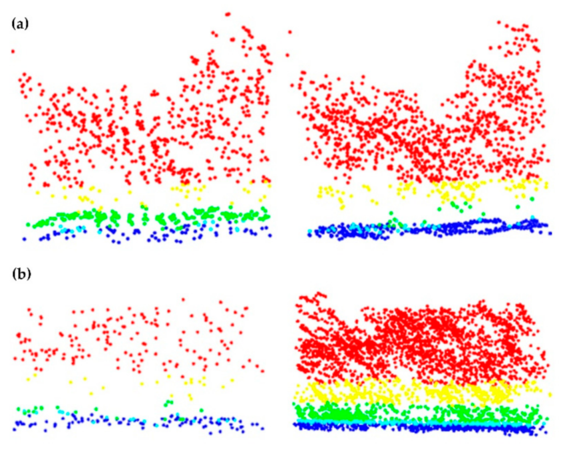
Figure 4.
Comparison of a vertical vegetation profile between 2010 (left) and 2016 (right) in a same cell. (a) Shows how a vegetation profile changed from forest with shrubs (FT6) in 2010 to forest with no understory (FT5) in 2016. (b) Displays the transition from forest with no understory (FT5) in 2010 to forest with vertical continuity (FT7) in 2016. Colors signify strata: above 4.0 m (red), 2.0–4.0 m (yellow), 0.6–2.0 m (green), 0.3–0.6 m (light blue), or below 0.3 m (dark blue).


Table 1.
Description of the different fuel types according to the Prometheus classification system [50].
Table 1.
Description of the different fuel types according to the Prometheus classification system [50].
| Average Shrub Height | Shrub Proportion | Average Distance between Understory and Tree Crowns | Description | Fuel Type | |
|---|---|---|---|---|---|
| Ground >60% | Pastures | FT1 | |||
| Canopy Cover | 0.3–0.6 m | >60% | Low shrubs | FT2 | |
| <50% | 0.6–2.0 m | >60% | Medium shrubs | FT3 | |
| (tree height >4.0 m) | 2.0–4.0 m | >60% | High shrubs | FT4 | |
| Canopy Cover | <30% | Forest without understory | FT5 | ||
| >50% | >30% | >0.5 m | Forest with shrubs | FT6 | |
| (tree height >4.0 m) | >30% | <0.5 m | Forest with vertical continuity | FT7 |
Table 2.
Fuel type classification system used for the LiDAR data.
| Ground | Cover | Mode | 2nd Mode | 3rd Mode | Max.Elev | Description | Fuel Type |
|---|---|---|---|---|---|---|---|
| >60% | Pastures | FT1 | |||||
| ≤60% | <50% | 0.0–0.3 m | Pastures | FT1 | |||
| 0.3–0.6 m | Low shrubs | FT2 | |||||
| 0.6–2.0 m | Medium shrubs | FT3 | |||||
| 2.0–4.0 m | High shrubs | FT4 | |||||
| >4.0 m | 0.0–0.3 m | Pastures | FT1 | ||||
| 0.3–0.6 m | Low shrubs | FT2 | |||||
| 0.6–2.0 m | Medium shrubs | FT3 | |||||
| 2.0–4.0 m | High shrubs | FT4 | |||||
| ≥50% | 0.0–0.3 m | Forest without understory | FT5 | ||||
| 0.3–0.6 m | Forest with shrub layer | FT6 | |||||
| 0.6–2.0 m | >12.0 m | Forest with shrub layer | FT6 | ||||
| ≤12.0 m | Forest with vertical continuity | FT7 | |||||
| 2.0–4.0 m | >12.0 m | Forest with shrub layer | FT6 | ||||
| ≤12.0 m | Forest with vertical continuity | FT7 | |||||
| >4.0 m | 0.0–0.3 m | Forest without understory | FT5 | ||||
| 0.3–0.6 m | Forest with shrub layer | FT6 | |||||
| 0.6–2.0 m | >12.0 m | Forest with shrub layer | FT6 | ||||
| ≤12.0 m | Forest with vertical continuity | FT7 | |||||
| 2.0–4.0 m | 0.0–0.3 m | Forest without understory | FT5 | ||||
| 0.3–0.6 m | Forest with shrub layer | FT6 | |||||
| 0.6–2.0 m | Forest with vertical continuity | FT7 |
Table 3.
Error matrix corresponding to the 2010 dataset. Accuracy measures are presented with a 95% confidence interval.
Table 3.
Error matrix corresponding to the 2010 dataset. Accuracy measures are presented with a 95% confidence interval.
| Reference Data | |||||||||||
|---|---|---|---|---|---|---|---|---|---|---|---|
| Classified Data | FT1 | FT2 | FT3 | FT4 | FT5 | FT6 | FT7 | Total | Map Area (ha) | User’s Accuracy | Producer’s Accuracy |
| Pasture (FT1) | 12 | 3 | 15 | 128.24 | 0.80 ± 0.21 | 0.99 ± 0.00 | |||||
| Low shrubs (FT2) | 1 | 10 | 2 | 2 | 15 | 3.72 | 0.67 ± 0.25 | 0.09 ± 0.09 | |||
| Medium shrubs (FT3) | 13 | 2 | 15 | 14.32 | 0.87 ± 0.18 | 0.96 ± 0.05 | |||||
| High shrubs (FT4) | 13 | 2 | 15 | 19.96 | 0.87 ± 0.18 | 0.90 ± 0.12 | |||||
| Forest without understory (FT5) | 12 | 2 | 1 | 15 | 197.24 | 0.80 ± 0.21 | 0.99 ± 0.01 | ||||
| Forest with shrubs (FT6) | 13 | 2 | 15 | 29.88 | 0.87 ± 0.18 | 0.48 ± 0.31 | |||||
| Forest with vertical continuity (FT7) | 1 | 4 | 10 | 15 | 6.64 | 0.67 ± 0.25 | 0.18 ± 0.21 | ||||
| Total | 13 | 13 | 15 | 15 | 13 | 21 | 15 | 105 | 400.00 | Overall accuracy | 0.81 ± 0.12 |
Table 4.
Error matrix corresponding to the 2016 dataset. Accuracy measures are presented with a 95% confidence interval.
Table 4.
Error matrix corresponding to the 2016 dataset. Accuracy measures are presented with a 95% confidence interval.
| Reference Data | |||||||||||
|---|---|---|---|---|---|---|---|---|---|---|---|
| Classified Data | FT1 | FT2 | FT3 | FT4 | FT5 | FT6 | FT7 | Total | Map Area (ha) | User’s Accuracy | Producer’s Accuracy |
| Pasture (FT1) | 12 | 2 | 1 | 15 | 112.52 | 0.80 ± 0.21 | 0.99 ± 0.00 | ||||
| Low shrubs (FT2) | 8 | 2 | 3 | 13 | 0.52 | 0.62 ± 0.28 | 0.99 ± 0.00 | ||||
| Medium shrubs (FT3) | 15 | 15 | 28.4 | 1.00 ± 0.00 | 0.49 ± 0.29 | ||||||
| High shrubs (FT4) | 13 | 2 | 15 | 12.76 | 0.87 ± 0.18 | 0.60 ± 0.47 | |||||
| Forest without understory (FT5) | 1 | 12 | 2 | 15 | 217.68 | 0.80 ± 0.21 | 0.99 ± 0.00 | ||||
| Forest with shrubs (FT6) | 9 | 6 | 15 | 12.24 | 0.60 ± 0.26 | 0.19 ± 0.20 | |||||
| Forest with vertical continuity (FT7) | 2 | 13 | 15 | 15.88 | 0.87 ± 0.18 | 0.67 ± 0.14 | |||||
| Total | 12 | 8 | 20 | 14 | 12 | 13 | 24 | 103 | 400.00 | Overall accuracy | 0.81 ± 0.13 |
Table 5.
Summary of the FT transitions between 2010 and 2016 with a pixel size of 20 m. Area changes per FT: proportion of area change per FT between 2010 and 2016 (%). Permanent since 2010: proportion of 2016 FT area that remained unchanged since 2010 (%). Permanent until 2016: proportion of 2010 FT area that remains unchanged until 2016 (%).
| Classified in 2010 | Permanent Since 2010 (%) | ||||||||
|---|---|---|---|---|---|---|---|---|---|
| Classified in 2016 | FT1 | FT2 | FT3 | FT4 | FT5 | FT6 | FT7 | Total | |
| Pasture (FT1) | 2510 | 83 | 117 | 66 | 30 | 1 | 6 | 2813 | 89.2 |
| Low shrubs (FT2) | 11 | 0 | 0 | 0 | 2 | 0 | 0 | 13 | 0.0 |
| Medium shrubs (FT3) | 435 | 8 | 154 | 106 | 3 | 3 | 1 | 710 | 21.7 |
| High shrubs (FT4) | 69 | 0 | 61 | 187 | 1 | 0 | 1 | 319 | 58.6 |
| Forest without understory (FT5) | 130 | 0 | 10 | 54 | 4470 | 688 | 90 | 5442 | 82.1 |
| Forest with shrubs (FT6) | 18 | 1 | 10 | 8 | 194 | 30 | 29 | 290 | 10.3 |
| Forest with vertical continuity (FT7) | 33 | 1 | 6 | 78 | 231 | 12 | 52 | 413 | 12.6 |
| Total | 3206 | 93 | 358 | 499 | 4931 | 734 | 179 | 10,000 | |
| Permanent until 2016 (%) | 78.3 | 0.0 | 43.0 | 37.5 | 90.7 | 4.1 | 29.1 | 74.0 | |
| Area changes per FT (%) (100% = no change) | 87.7 | 14.0 | 198.3 | 63.9 | 110.4 | 39.5 | 230.7 | ||
Table 6.
Observed frequencies of the following factors: forest fuel type (FT; FT5, FT6, and FT7), forest vegetation cover type (beech, pine, oak and mixed deciduous) and aspect (sunny and shady) in 2016 in the study area. Statistically significant frequencies (p < 0.05) have been identified with an asterisk (*).
| Forest Vegetation Cover Types (%) | |||||||
|---|---|---|---|---|---|---|---|
| Fuel Type (FT) | Aspect | Beech | Pine | Oak | Mixed Deciduous | Total | Aggregated |
| Forest without understory (FT5) | Sunny | 9.5 * | 2.3 | 6.5 * | 1.5 | 19.8 | 88.6 |
| Shady | 58.0 * | 6.2* | 2.9 | 1.7 | 68.7 | ||
| Forest with shrubs (FT6) | Sunny | 0.8 | 0.1 | 1.5 | 0.0 | 2.4 | 4.7 |
| Shady | 1.7 | 0.4 | 0.1 | 0.0 | 2.3 | ||
| Forest with vertical continuity (FT7) | Sunny | 0.9 | 0.0 | 3.9 * | 0.0 | 4.9 | 6.7 |
| Shady | 1.3 | 0.1 | 0.4 | 0.0 | 1.8 | ||
| Total | 72.2 | 9.2 | 15.4 | 3.3 | 100.0 | ||
Table 7.
Changes among structural stand and fuel types (FT5: forest without understory; FT6: forest with shrubs; FT7: forest with vertical continuity), forest vegetation cover types (beech, oak, pine and mixed deciduous forest) and aspect (sunny and shady). Statistically significant frequencies (p < 0.05) have been identified with an asterisk (*).
| Forest Vegetation Cover Type (%) | ||||||
|---|---|---|---|---|---|---|
| FT Changes | Aspect | Beech | Pine | Oak | Mixed | Total |
| FT5-->FT6 | Sunny | 3.4 | 0.3 | 5.4 * | 0.0 | 9.1 |
| Shady | 5.1 * | 1.2 | 0.1 | 0.2 | 6.5 | |
| FT5-->FT7 | Sunny | 2.7 | 0.2 | 11.7 * | 0.1 | 14.6 |
| Shady | 2.7 | 0.4 | 0.8 | 0.1 | 3.9 | |
| FT6-->FT5 | Sunny | 15.8 * | 0.0 | 2.0 | 0.0 | 17.8 |
| Shady | 36.6 * | 0.7 | 0.2 | 0.0 | 37.5 | |
| FT6-->FT7 | Sunny | 0.2 | 0.0 | 0.4 | 0.0 | 0.6 |
| Shady | 0.2 | 0.0 | 0.2 | 0.0 | 0.3 | |
| FT7-->FT5 | Sunny | 1.3 | 0.0 | 1.6 | 0.0 | 2.9 |
| Shady | 2.6 | 1.2 | 0.5 | 0.1 | 4.3 | |
| FT7-->FT6 | Sunny | 0.0 | 0.0 | 1.0 | 0.0 | 1.0 |
| Shady | 0.9 | 0.2 | 0.2 | 0.1 | 1.4 | |
| Total (%) | 71.3 | 4.3 | 24.0 | 0.5 | 100.0 | |
Publisher’s Note: MDPI stays neutral with regard to jurisdictional claims in published maps and institutional affiliations. |
© 2021 by the authors. Licensee MDPI, Basel, Switzerland. This article is an open access article distributed under the terms and conditions of the Creative Commons Attribution (CC BY) license (http://creativecommons.org/licenses/by/4.0/).
Share and Cite
MDPI and ACS Style
García-Cimarras, A.; Manzanera, J.A.; Valbuena, R. Analysis of Mediterranean Vegetation Fuel Type Changes Using Multitemporal LiDAR. Forests 2021, 12, 335. https://doi.org/10.3390/f12030335
AMA Style
García-Cimarras A, Manzanera JA, Valbuena R. Analysis of Mediterranean Vegetation Fuel Type Changes Using Multitemporal LiDAR. Forests. 2021; 12(3):335. https://doi.org/10.3390/f12030335
Chicago/Turabian StyleGarcía-Cimarras, Alba, José Antonio Manzanera, and Rubén Valbuena. 2021. "Analysis of Mediterranean Vegetation Fuel Type Changes Using Multitemporal LiDAR" Forests 12, no. 3: 335. https://doi.org/10.3390/f12030335
Note that from the first issue of 2016, this journal uses article numbers instead of page numbers. See further details here.