Multi-Time Scale Evaluation of Forest Water Conservation Function in the Semiarid Mountains Area

Abstract

Forest water conservation function is an important part of forest ecosystem services. The discontinuous distribution of forests in semiarid areas brings difficulties to the quantitative evaluation of forest water conservation functions at the basin scale. In this paper, we took the upstream of Xiong’an New Area (Zijingguan—ZJG, Zhongtangmei—ZTM and Fuping—FP basins) as an example and combine the soil and water assessment tool (SWAT) and the water balance method to calculate the amount of forest water conservation (AFWC) at annual, monthly and daily scales from 2007 to 2017, and analyzed the changes of AFWC. The results showed that the hydrological response unit (HRU) generated with the threshold area zero can accurately reflect the forest patch distribution in the three basins. On an annual scale, the annual AFWC were all positive in ZJG and ZTM basins from 2007 to 2017. While, the annual AFWC in the FP basin was negative in 2009, 2013, 2014 and 2017. On a monthly scale, the positive values of AFWC mainly appear from June to September, and the negative values of AFWC mainly appear from December to March. On a daily scale, the AFWC during extreme precipitation was positive, while that was negative during extreme drought. The annual and monthly AFWC in the three basins was positively correlated with the wetness index, and FP basin needs more humid climate conditions than ZJG and ZTM basins to make the forest store water and keep in a stable water storage state. The above results can not only provide important insight into sustainable forest and water resources management in the region, but also serve as reference cases for other regions to carry out relevant research work.

1. Introduction

Water is the source of life, the essentials of production and the foundation of the ecosystem [1,2]. In the era of low human productivity, people have relatively low productive and domestic needs for water, and the main task is the development and utilization of water resources [3]. With the continuous improvement of human production and living standards, the demand for water resources has gradually increased [4]. Therefore, the main task becomes the development and conservation of water resources. Along with that, climate warming and other environmental problems have appeared, water shortage and drought and flood disasters frequently alternate in different regions, years and seasons worldwide [5,6]. At this time, the main task is the rational development and efficient utilization of water resources, producing water conservation. The concept of water conservation refers to the process and ability of the ecosystem to water stored or retained within a specific time and space [7]. Meanwhile, the stored water will be discharged to feed the ecological base flow of the basin in the non-rainy season and provide a strong guarantee for the water used by social development and human life [8]. Forests play a role in water conservation on different time scales through a forest canopy, litter layer and soil layer [9,10,11]. The water conservation of forests is usually quantified by the amounts of forest water conservation (AFWCs) [12]. Most studies are based on the fixed-point experimental observation methods to study forest water conservation on the individual plant and slope scale, and there is a lack of studies on the water conservation of forests at larger spatial scales [13,14].

The main methods for calculating the AFWC mainly include canopy interception, integrated storage capacity and water balance methods. Specifically, the canopy interception method estimates the AFWC by measuring the canopy interception rate of different forest vegetation in the experimental plots [15,16]. The integrated storage capacity method estimates the AFWC by calculating the precipitation interception parameters at different layers of the forest in the experimental plots [17,18]. However, different calculation methods inevitably have their own advantages, characteristics, and limitations. The above methods can calculate the AFWC on multitime scales, but because the forest evapotranspiration and surface runoff are ignored, the calculation results are often greater than the actual water conservation amount [19]. Additionally, the above methods are aimed at basins where the forest area accounts for a large proportion of the basin area. However, for semiarid mountainous areas in Northern China, the spatial distribution of forests is discontinuous under the influence of temperature and precipitation, and the proportion of forest area is far from large enough to ignore other land use types [20,21]. Therefore, the water conservation amount of the basin cannot be equal to the AFWC. The water balance method is widely used for basin scales, which takes water, soil and forest in the basins as a whole, and defines the difference between the precipitation of the basin and forest evaporation and other consumption as the amount of water conservation according to the principle of water balance [22,23]. The water balance method is the basis of studying the mechanism of water conservation and can calculate the water conservation amount more accurately [19]. Compared with other methods, it is a relatively mature and accurate method to evaluate the water conservation function of the forest ecosystem. The current research mainly combines the water balance method with remote sensing and hydrological models to study the difference in AFWC and its spatial distribution in the basin [24,25]. However, most of the existing studies use the average annual runoff to calibrate the model parameters and obtain the average multiyear value of AFWC, which not reflects the AFWC at smaller time scales [26,27,28].

In addition, the manifestations of forest water conservation may be different on different time scales. Previous studies have shown that the response of rainfall runoff processes to land use is different at different time scales [29], and the characteristics of precipitation and evapotranspiration on different time scales are different [2,30]. In the semiarid monsoon region, precipitation is uneven during the year, and short term heavy precipitation is prone to occur [31]. Therefore, the calculation and analysis of AFWC on different time scales can be helpful in evaluating the role of forest water conservation in flood interception and runoff regulation in semiarid monsoon areas more comprehensively.

Ecohydrological modeling is an indispensable tool in understanding the interaction of hydrological processes and environmental issues [32]. The soil and water assessment tool (SWAT) ecohydrological models have a strong physical mechanism, which simulating and analyzing the temporal and spatial changes of hydrological processes such as interception, evapotranspiration, infiltration, surface runoff and groundwater runoff from the time scale of a year, month and day [33,34,35]. Moreover, the SWAT can reflect the spatiotemporal variability of climate factors and the underlying surface and has been widely applied in the research of forest hydrology [36,37]. Therefore, the combination of the SWAT model and water balance method can quantitatively analyze the multitime scale characteristics of forest water conservation [38].

The upstream of Xiong’an New Area is located in a temperate monsoon climate zone [39]. The intermonthly changes of climate factors such as precipitation and evapotranspiration in the region are large, and short term heavy precipitation and continuous drought are prone to occur on a daily scale [40]. The landform is dominated by hills and mountains, and forests play an important role in water conservation at different time scales [39]. Meanwhile, the SWAT model has good applicability in the upstream of Xiong’an New Area [41,42]. On 1st April 2017, the Chinese government officially announced the establishment of Xiong’an New Area to centralize the relief of some extra capital functions from Beijing [43]. The water supply safety and flood controlling ability of Xiong’an New Area largely depend on flood interception and runoff regulation capacity of its upstream ecosystem. The main land use types in the upstream of Xiong’an New Area are grassland and forest [44], and forests have stronger flood interception and runoff regulation ability than grasslands [45,46]. This puts forward higher requirements for the study of the forest water conservation in the upper reaches of Xiong’an New Area. Therefore, we take the upstream of Xiong’an New Area as the study area, divide the forest HRUs according to the forest distribution characteristics in the study area and construct a SWAT hydrological model, which reflects the forest distribution characteristics in the basin, then calculate the AFWC on different time scales according to the principle of water balance.

This research provides new ideas for a theoretical basis of the formulation and adjustment of water resources management policies and ecological environment policies in the upstream of Xiong’an New Area as well.

2. Materials and Methods

2.1. Overview of the Study Area

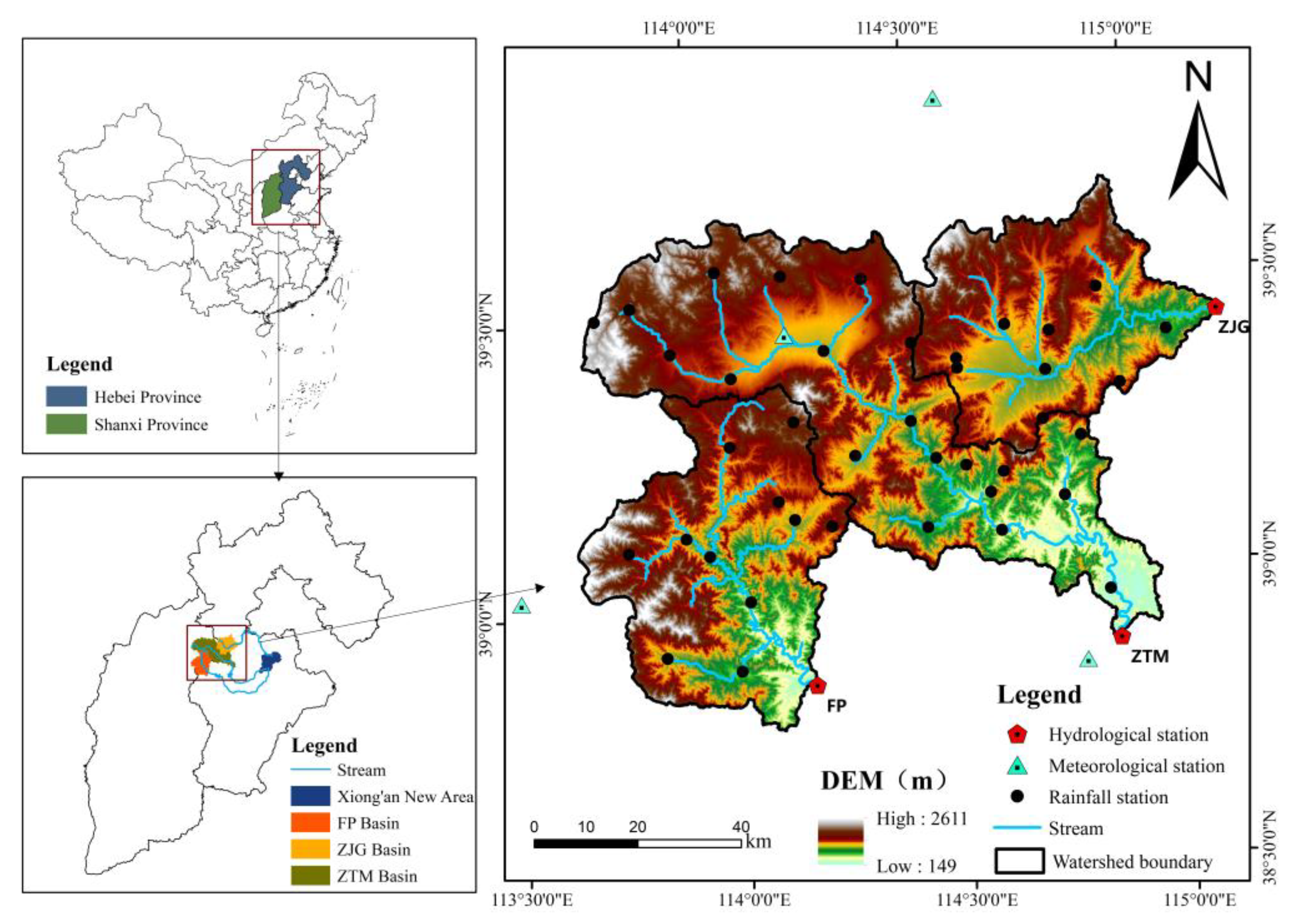
The study area is located in 38°46′31″–39°40′8″ N and 113°40′4″–115°10′1″ E, and includes three basins in the upstream of Xiong’an New Area, across Hebei and Shanxi provinces of the Northern China, Zijingguan (ZJG), Zhongtangmei (ZTM) and Fuping (FP) basins, with a total area of 7310.27 km² (Figure 1).

Table 1. The main underlying surface characteristics of the ZJG, ZTM and FP basins.

Basins	Main Land Use Types	Main Soil Types	Average Slope
ZJG	Forest land (42.00%)	Cinnamon Soil (86.20%)	17.75°
	Grassland (33.83%)
ZTM	Grassland (50.20%)	Cinnamon Soil (77.56%)	17.76°
	Forest land (26.11%)
FP	Grassland (53.96%)	Cinnamon Soil (92.35%)	22.25°
	Forest land (39.40%)

shows the main underlying surface characteristics of the three basins. The terrain of the study area is high in the northwest and low in the southeast, with an average altitude of 1108 m and an average slope of about 19°, which belongs to the mountainous hilly area. The study area belongs to the monsoon climate of medium latitudes zone with an average annual temperature of 7.4–12.8 °C and annual precipitation of 550–790 mm [39]. Affected by the monsoon climate, precipitation in the study area was uneven throughout the year, nearly 80% was concentrated from June to September [40].

2.2. Data Sources

The daily runoff data from 2006 to 2017 at three hydrological stations in Zijingguan, Zhongtangmei and Fuping (Figure 1) were obtained from the hydrological yearbook of the Haihe River basin. The daily precipitation data of 42 rainfall stations and four national meteorological stations in the basin from 2006 to 2017 were provided by the hydrological yearbook of the Haihe River basin and China Meteorological Data Network, respectively. Other meteorological data, such as maximum temperature, average temperature, minimum temperature, solar radiation, wind speed and relative humidity were also provided by the China Meteorological Data Network for the period of 2006–2017. The soil type data was obtained from the Cold and Arid Region Scientific Data Center of the Chinese Academy of Sciences (http://data.casnw.net/portal/, accessed on 23 December 2020), with a spatial resolution of 1 km × 1 km, including soil depth, soil texture, organic substances content in the soil, soil bulk density and other attribute data that affect soil moisture movement. The hydrological properties of the soil were calculated based on the soil water characteristic software Soil Plant Atmosphere Water (SPAW) developed by the United States Department of Agriculture. The land use data for 2010 was provided by the Resource and Environmental Science Data Center of the Chinese Academy of Sciences (http://www.resdc.cn/, accessed on 23 December 2020) with a spatial resolution of 100 m × 100 m. Digital elevation model (DEM) data were downloaded in the Geospatial Data Cloud (http://www.gscloud.cn/, accessed on 23 December 2020), with a spatial resolution of 30 m × 30 m. This work was guided on “Observation Methodology for Longterm Forest Ecosystem Re-search” of the National Standards of the People’s Republic of China (GB/T 33027-2016).

2.3. Construction of the SWAT Model

2.3.1. Division of Hydrological Response Units

In applications of the SWAT model, the stream structure is first extracted using the DEM data, and the whole basin is divided into several sub-basins. Then, the Hydrological Response Units (HRUs) are generated by overlaying land use types, soils map, and slope distribution [47,48]. The HRUs comprise the basic calculation unit of the SWAT model, representing the unique combination of land cover, soil type, and slope class within a sub-basin [49,50]. In order to make all land use types, soil types and slopes participate in the simulation of the model, the area threshold of land use, soil and slope in this paper was set as 0 [38]. We selected the HRU of the forest for water conservation calculation and define the HRU of the forest as FHRU. Based on the generated HRU vector data, FHRU was screened out through the field of land use. The relevant statistical results were combined with HRUGIS code to obtain the spatial distribution map of FHRU [38].

2.3.2. Model Construction and Parameter Calibration

The soil conservation service (SCS) runoff curve model was used to calculate surface runoff, the Penman–Monteith formula was used to calculate reference evapotranspiration in the basin, the dynamic water storage reservoir model was used to calculate lateral flow, and the basal flow regression coefficient method was used to calculate groundwater runoff [51]. The global sensitivity analysis module of SWAT-CUP 2012 was adopted to analyze parameter sensitivity. According to the results of sensitivity analysis, 10 parameters with greater sensitivity were selected (

Table 2. Parameter screening results.

Parameter	Description	Range
ALPHA_BF	Baseflow alpha factor (day)	0–1
CH_K2	Effective hydraulic conductivity in main channel alluvium (mm/h)	−0.01–500
CN2	SCS curve number for moisture condition	−0.3–0.3
ESCO	Soil evaporation compensation factor	0.4–1
SOL_K	Saturated hydraulic conductivity	−0.3–0.3
GWQMN	Threshold depth of water in the shallow aquifer required for return flow to occur (mm)	0–1500
SURLAG	Surface runoff lag coefficient (day)	0.05–24
REVAPMN	Threshold depth of water in the shallow aquifer for “revap” to occur (mm)	0–500
GW_DELAY	Groundwater delay (day)	30–450
SOL_AWC	Available water capacity of the soil layer	−0.3–0.3

).

Model performance assessment is essential to model selection and utilization. The Nash–Sutcliffe ($NSE$) [52], correlation coefficient ($R^2$) [53] and relative bias (PBIAS) [54] were used to evaluate the simulation results. Specifically, NSE was used to characterize the degree of fit between the simulated value and the observed value; PBIAS was used to calculate the gap between the simulated value and the measured value; $R^2$ was used to evaluate the consistency of the changing trend between the measured value and the simulated value sequence. Generally, when NSE ≥ 0.5, $R^2$ ≥ 0.6, and |PBIAS| ≤ 25%, the simulation results of the model are considered credible [55]. The calculated formula was as follows,

$$NSE=1-\frac{{\sum }_{i=1}^n{( Q_i^{obs}- Q_i^{sim})}^2}{{\sum }_{i=1}^n{( Q_i^{obs}- Q_{avg}^{obs})}^2}$$

(1)

$$R^2=\frac{{\left[{\sum }_{i=1}^n( Q_i^{obs}- Q_{avg}^{obs})( Q_i^{sim}- Q_{avg}^{sim})\right]}^2}{{\sum }_{i=1}^n{( Q_i^{obs}- Q_{avg}^{obs})}^2{\sum }_{i=1}^n{( Q_i^{sim}- Q_{avg}^{sim})}^2}$$

(2)

$$PBIAS=\frac{{\sum }_{i=1}^n( Q_i^{obs}- Q_i^{sim})}{{\sum }_{i=1}^n{Q}_i^{obs}}$$

(3)

where $Q_i^{obs}$ and $Q_i^{sim}$ are the observed and simulated values of runoff respectively and $Q_{avg}^{obs}$ and $Q_{avg}^{sim}$ are the average values of the observed and simulated values of runoff respectively.

2.4. The Calculation Method of AFWC Based on the SWAT Model

From the water balance perspective, the difference between precipitation and forest evapotranspiration and other consumption is the AFWC [23,56]. Its expression is,

$$W=P-AET-R$$

(4)

where W is the amount of forest water conservation (mm) and $P$, $AET$ and R are precipitation, actual evapotranspiration and surface runoff (mm), respectively.

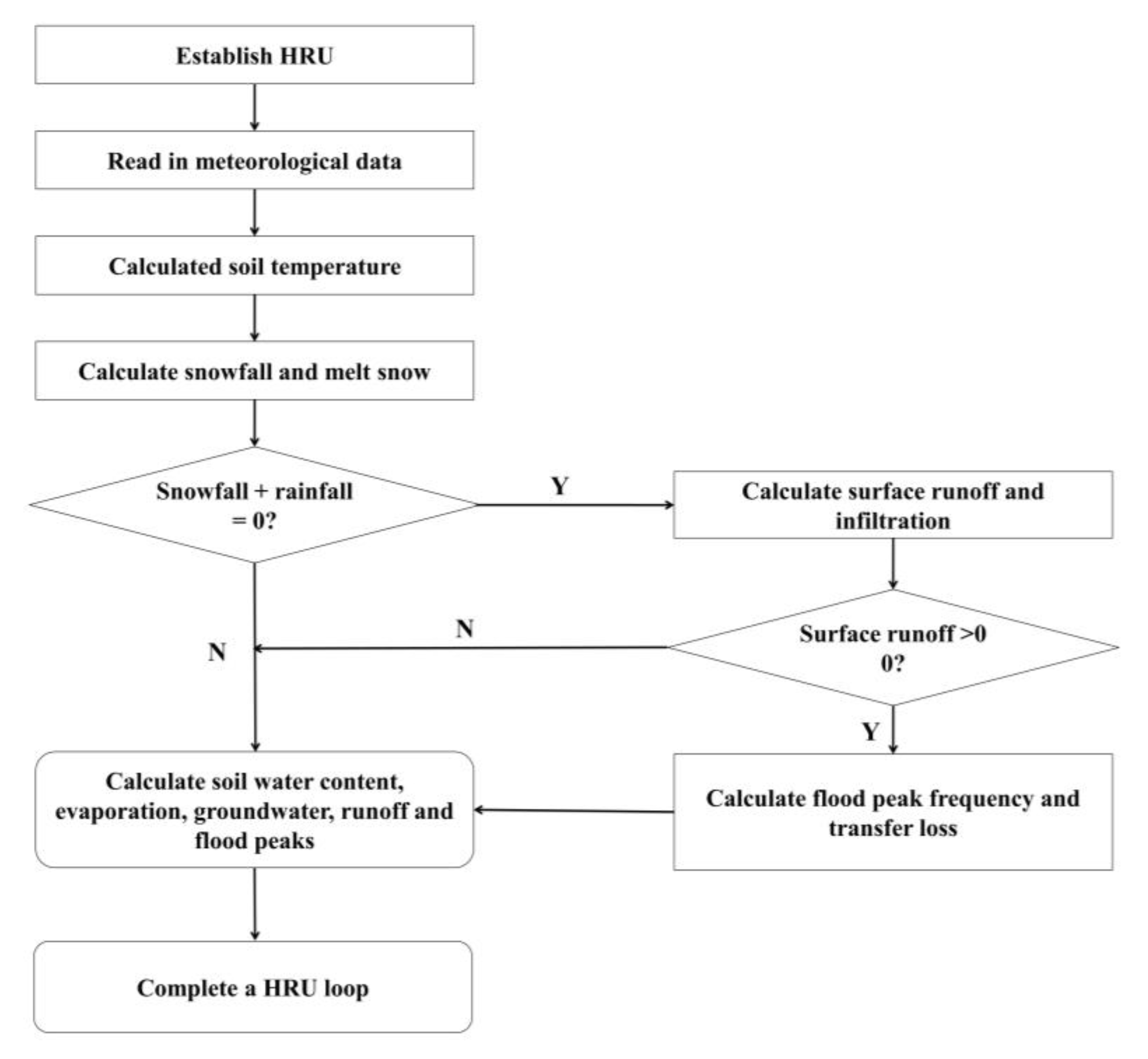
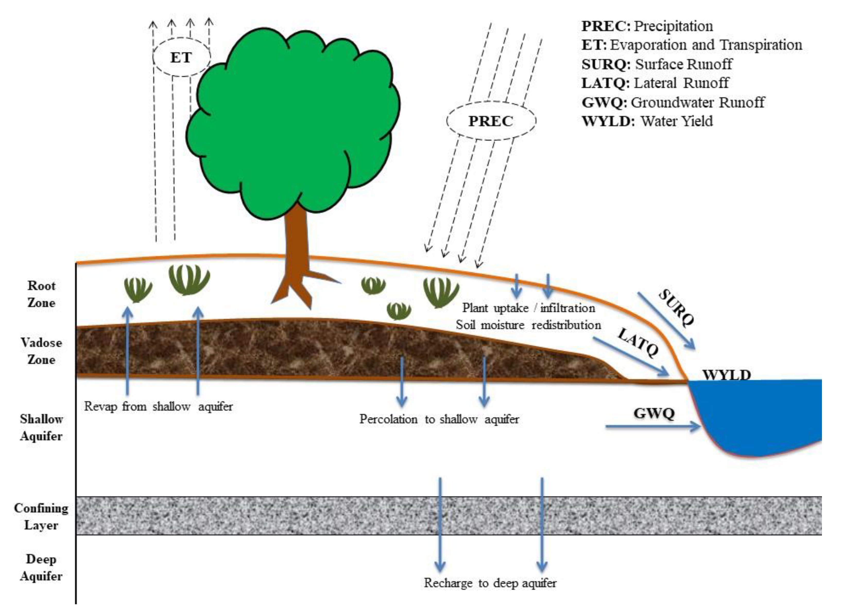
The SWAT model used the hydrological response unit (HRU) as the minimum simulation unit to simulate hydrological cycle processes (Figure 2). The forest hydrological process based on the SWAT model can be summarized as Figure 3. The water balance equation based on the SWAT model can be expressed as [38],

$$\Delta S_i=PRE{C}_i-AE{T}_i-WYL{D}_i$$

(5)

$$WYL{D}_i=SUR{Q}_i+LAT{Q}_i+GW{Q}_i$$

(6)

where $i$ is the ith HRU, $\Delta S_i$ is the amount of water change on the ith HRU, $PRE{C}_i$ is the ith HRU precipitation and $AE{T}_i$ is the ith HRU actual evapotranspiration and $WYL{D}_i$ represents the amount of water flowing from the ith HRU. $SUR{Q}_i$ represents the surface runoff of the ith HRU, $LAT{Q}_i$ represents the lateral flow of the ith HRU and $GW{Q}_i$ represents the groundwater runoff of the ith HRU.

The water conservation amount $Y_i$ of the ith FHRU can be expressed as,

$$Y_i=PRE{C}_i-\mathrm{A}E{T}_i-SUR{Q}_i$$

(7)

The water conservation amount of the ith FHRU in the basin based on the SWAT model can be calculated according to the following formula [38,57],

$$W_{ij}={\displaystyle \sum }_{i=1}^n\left(PRE{C}_{ij}-AE{T}_{ij}-SUR{Q}_{ij}\right)\times S_i\times 1000$$

(8)

where $W_{ij}$ is the water conservation amount of the ith FHRU (m³), $PRE{C}_{ij}$ is the precipitation of the ith FHRU (mm), $AE{T}_{ij}$ is the actual evapotranspiration of the ith FHRU (mm), $SUR{Q}_{ij}$ is the surface diameter of the ith FHRU flow (mm), $S_i$ represents the area of the ith FHRU (km²) and $j$ represents the value corresponding to the time scale of a year, month, and day.

The water conservation amount of all FHRU was summed up to obtain the forest water conservation amount $W_j$ of the whole basin in a specific time scale, which can be expressed as,

$$W_j={\displaystyle \sum }_{i=1}^n{W}_{ij}$$

(9)

where n is the total number of FHRUs in the basin and $j$ represents the value corresponding to the time scale of a year, month and day.

2.5. Selection of Daily Time Scale Eigenvalues

On a daily scale, we mainly study the change characteristics of AFWC during extreme precipitation and extreme drought. The day with the largest precipitation and the three days with the largest continuous precipitation were selected to represent the period of extreme precipitation. The reason why selecting three consecutive days was that the flood duration of the basin was generally about three days [58]. The day with the smallest AFWC and the seven days with the smallest continuous AFWC were selected to represent the period of extreme drought.

3. Results

3.1. Spatial Distribution of FHRU

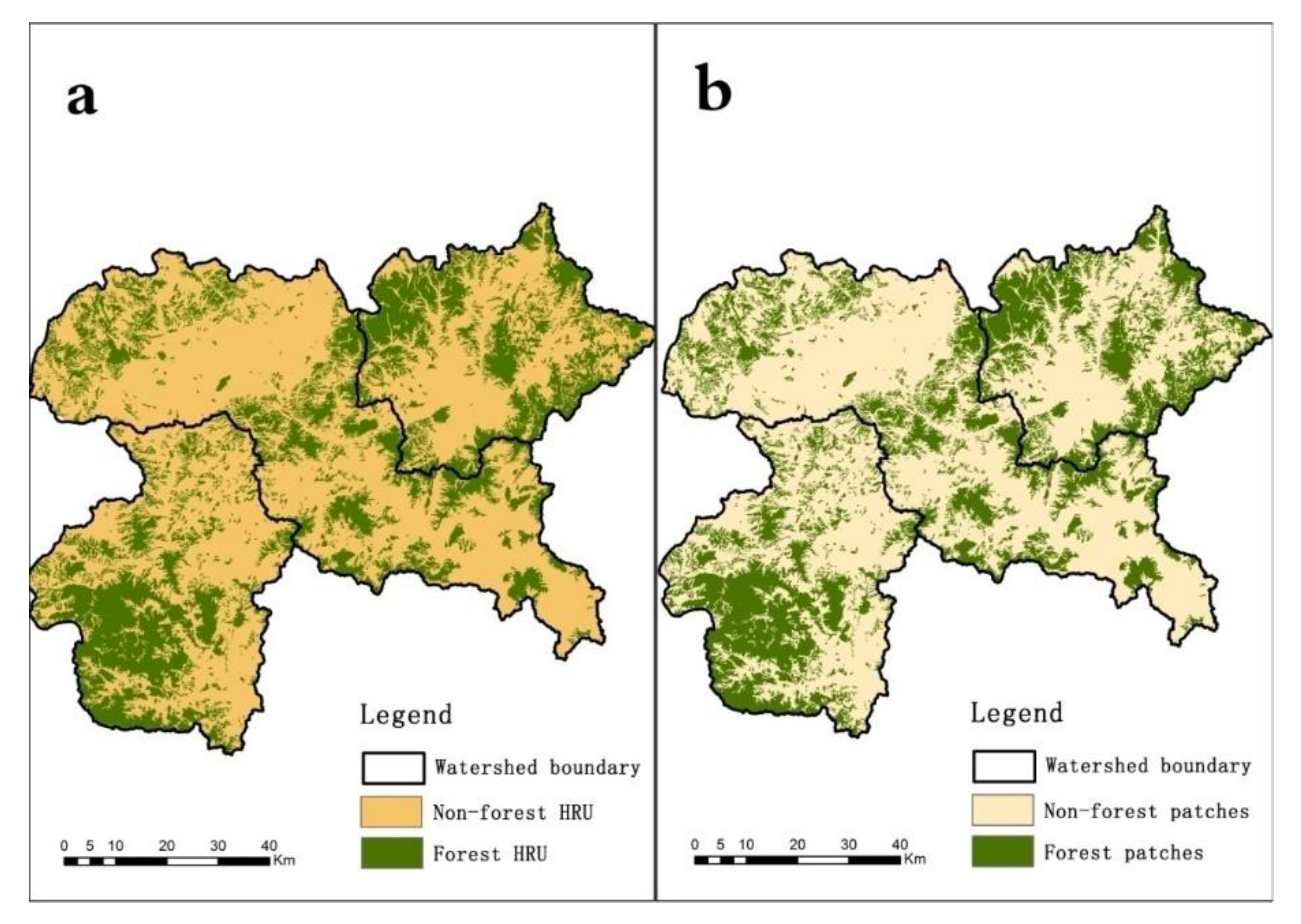
The SWAT model established in this study generated 702, 1572 and 829 HRUs in ZJG, ZTM and FP basins respectively. The actual forest area of ZJG, ZTM and FP basins was basically consistent with the generalized area of the model, as shown in

Table 3. Comparison of different land use HRUs with actual patches in the ZJG basin when the area threshold is set to 0.

Land Use Types	Actual Area (km2)	Generalized Area (km2)	Actual Proportion (%)	Generalized Proportion (%)	Number of HRU
Arable land	348.42	349.97	19.91	20.06	149
Forest land	735.07	728.31	42.00	41.75	151
Grassland	592.20	590.95	33.83	33.88	153
Waters	19.06	19.16	1.09	1.10	67
Construction land	53.96	54.30	3.08	3.12	175
Bare land	1.61	1.62	0.09	0.09	7
Total	1750.32	1744.31	100.00	100.00	702

,

Table 4. Comparison of different land use HRUs with actual patches in the ZTM basin when the area threshold is set to 0.

Land Use Types	Actual Area (km2)	Generalized Area (km2)	Actual Proportion (%)	Generalized Proportion (%)	Number of HRU
Arable land	681.35	682.79	20.01	20.11	333
Forest land	888.66	883.65	26.11	26.03	368
Grassland	1712.30	1704.57	50.20	50.21	402
Waters	55.78	56.07	1.64	1.65	192
Construction land	67.46	67.62	2.04	2.00	277
Bare land	0.00	0.00	0.00	0.00	0
Total	3405.55	3394.71	100.00	100.00	1572

and

Table 5. Comparison of different land use HRUs with actual patches in the FP basin when the area threshold is set to 0.

Land Use Types	Actual Area (km2)	Generalized Area (km2)	Actual Proportion (%)	Generalized Proportion (%)	Number of HRU
Arable land	97.53	97.98	4.53	4.56	129
Forest land	848.87	844.79	39.40	39.32	199
Grassland	1162.44	1160.22	53.96	54.00	205
Waters	22.69	22.77	1.05	1.06	115
Construction land	22.78	22.71	1.06	1.06	176
Bare land	0.09	0.07	0.00	0.00	5
Total	2154.40	2148.54	100.00	100.00	829

. The actual forest patch area was 735.07 km², 888.66 km² and 848.87 km² respectively, and the FHRU area after model generalization was 728.31 km², 883.65 km² and 844.79 km² respectively, with the difference of 0.92%, 0.56% and 0.48% respectively. In terms of basins, there were 151, 368 and 199 FHRUs in ZJG, ZTM and FP, respectively, accounting for 41.75%, 26.03% and 39.32% of their respective basin area respectively. The comparison of the spatial distribution of forest patches and FHRU, which reflects the spatial similarity between them was shown in Figure 4.

3.2. Model Calibration and Validation

The determination of calibration and validation periods affects the prediction accuracy of model simulation. In this study, the model warm-up period was 2006, the calibration period was 2007–2012, the validation period was 2013–2017 and the model parameters were calibrated and validated at the year, month and day scales.

Table 6. Model performance: calibrated and validated results for annual, monthly and daily runoff for ZJG, ZTM and FP basins.

Periods	Validation Indicator	Year			Month			Day
		ZJG	ZTM	FP	ZJG	ZTM	FP	ZJG	ZTM	FP
Calibration period (2007–2012)	NSE	0.87	0.86	0.89	0.83	0.84	0.82	0.78	0.77	0.79
	R2	0.92	0.9	0.9	0.87	0.86	0.87	0.82	0.84	0.82
	PBIAS (%)	−2.13	1.54	0.84	10.81	8.75	−1.93	7.97	5.62	2.8
Validation period (2013–2017)	NSE	0.88	0.85	0.87	0.82	0.8	0.81	0.74	0.78	0.77
	R2	0.9	0.88	0.89	0.84	0.85	0.85	0.81	0.82	0.81
	PBIAS (%)	5.1	8.43	3.3	5.77	8.4	4.59	−2.8	4.8	5.9

shows the comparison results of simulated and measured values of different time scales at three stations.

For annual scales, NSE and $R^2$ of the calibration and validation periods of the three stations were all greater than 0.85, and the absolute value of PBIAS were less than 10%. For monthly scales, the NSE and $R^2$ of the three stations in the calibration and validation periods were all greater than 0.8. With the exception of ZJG, which was 10.86%, the absolute value of PBIAS in the calibration period was less than 10% for the three stations. The absolute value of the PBIAS of the three stations in the validation period was less than 10%. For daily scales, the NSE and $R^2$ of the three stations in the calibration period were all greater than 0.75, and the PBIAS were all less than 10%. During the validation period, the NSE of the three stations were all greater than 0.7, $R^2$ were greater than 0.8, and the absolute value of the PBIAS was less than 10%. In general, the constructed model can reflect the hydrological cycle process at different time scales in the ZJG, ZTM and FP basins.

3.3. The Amount of Forest Water Conservation (AFWC) at Different Time Scales

3.3.1. Annual Conservation Amount

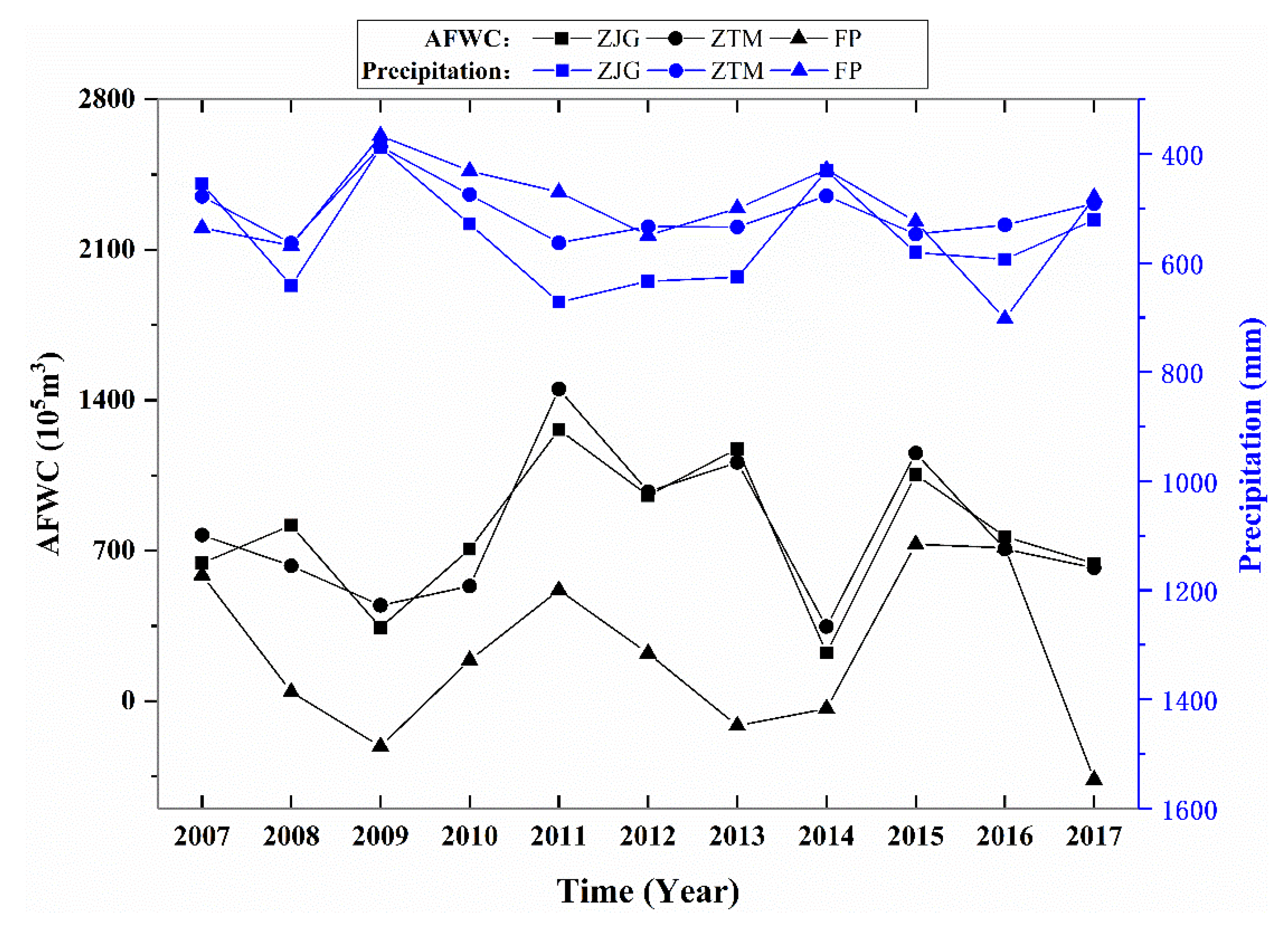
The interannual variation of AFWC in the study area was large (Figure 5). During the study period, the AFWC of the ZJG and ZTM basins was mostly positive, but the AFWC of the FP basin showed negative values in 2009, 2013, 2014 and 2017, the values were −211.15, −114.92, −35.27 and −365.98 (10⁵ m³) respectively.

The highest value of AFWC in the ZJG and ZTM basins appeared in 2011, with values of 1263.27 and 1452.43 (10⁵ m³), respectively. The lowest value of AFWC in the ZJG and ZTM basins appeared in 2014, with values of 224.78 and 346.25 (10⁵ m³), respectively. The lowest value of AFWC in the FP basin was −365.98 (10⁵ m³) in 2017, and the highest value in the FP basin was 729.07 (10⁵ m³) in 2015.

Moreover, it can be seen from Figure 5 that the changing trend of annual precipitation in each basin is similar to that of AFWC, which shows that precipitation is an important factor affecting water conservation.

3.3.2. Monthly Conservation Amount

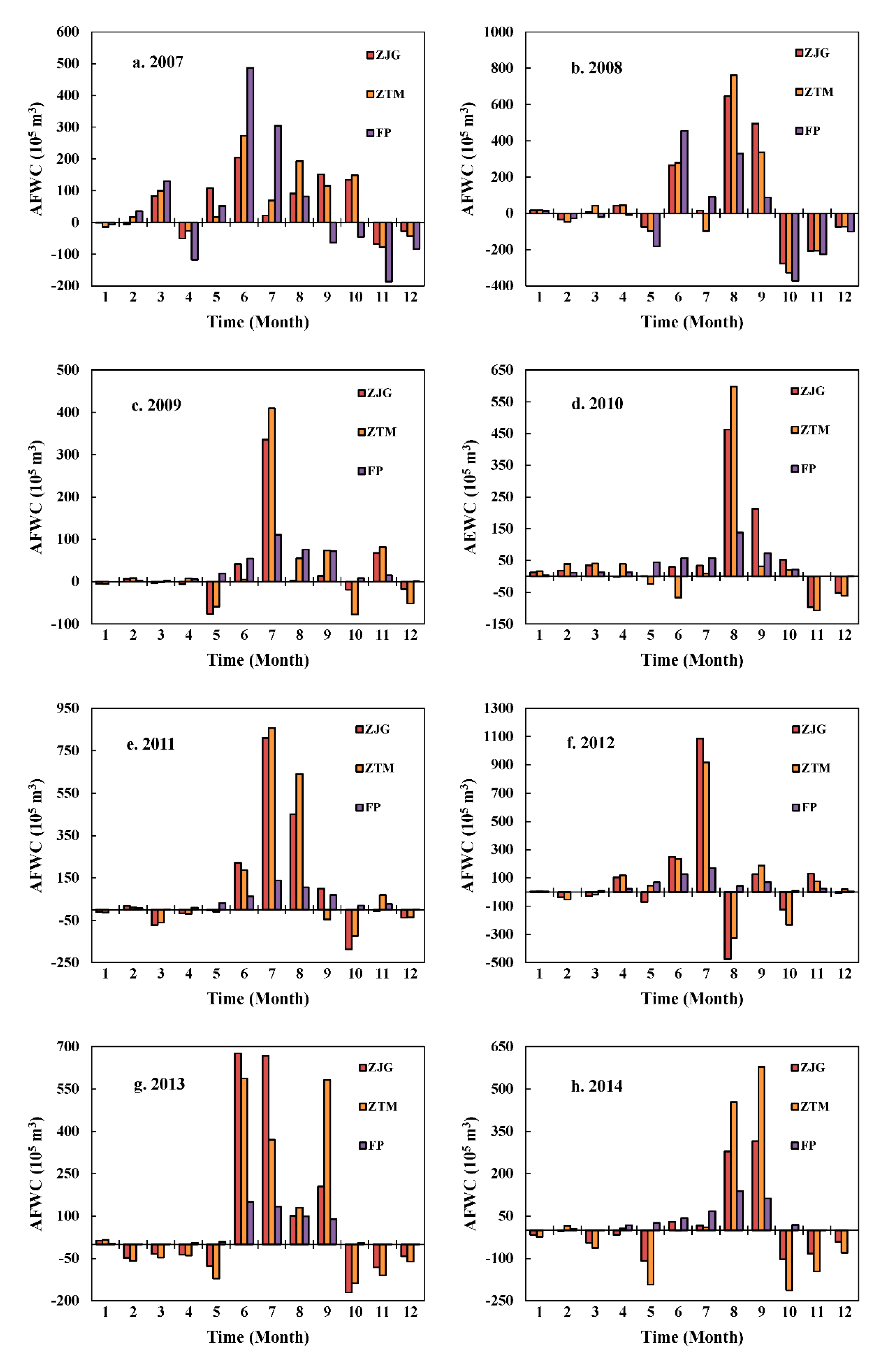
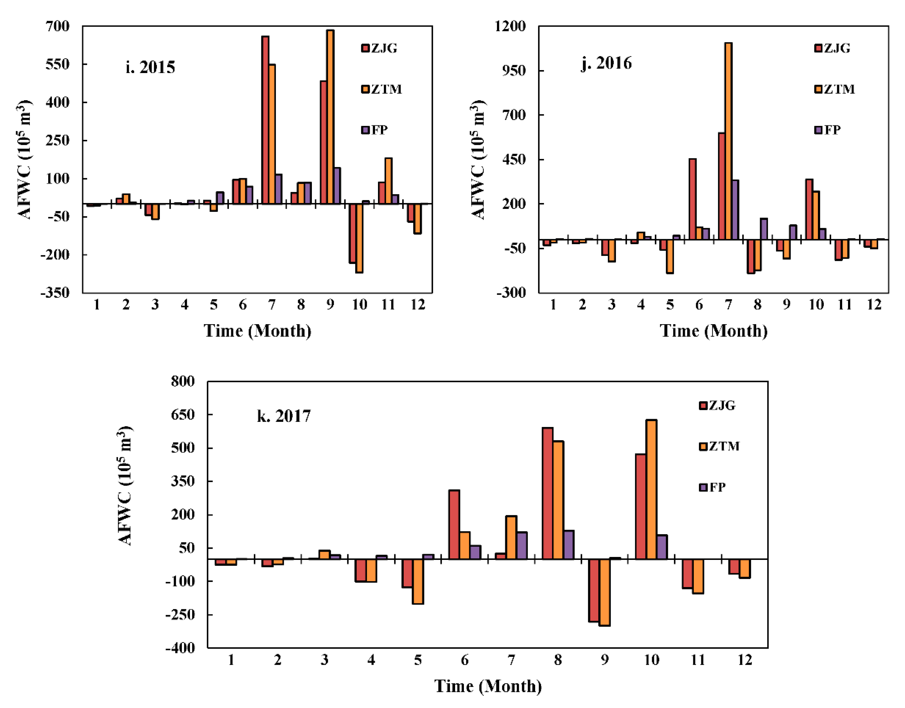
It can be seen from Figure 6 that the AFWC in different months varied greatly, which was reflected in the magnitude of the value and positive-negative changes. For the ZJG basin, the maximum AFWC was 1086.30 (10⁵ m³) in July 2012 and the minimum was −475.62 (10⁵ m³) in August 2012. For the ZTM basin, those two values were 1105.65 (10⁵ m³) in July 2016 and −328.17 (10⁵ m³) in October 2008. For the FP basin, the maximum AFWC was 487.13 (10⁵ m³) in June 2007, and the minimum AFWC was −372.61 (10⁵ m³) in October 2008.

The negative AFWC indicates that the AFWC in this month was in deficit. From 2007 to 2017, there were 67, 65 and 21 months with negative AFWC in ZJG, ZTM and FP basins, respectively, of which 47.76%, 44.62% and 52.38% occurred in December to March (Figure 6).

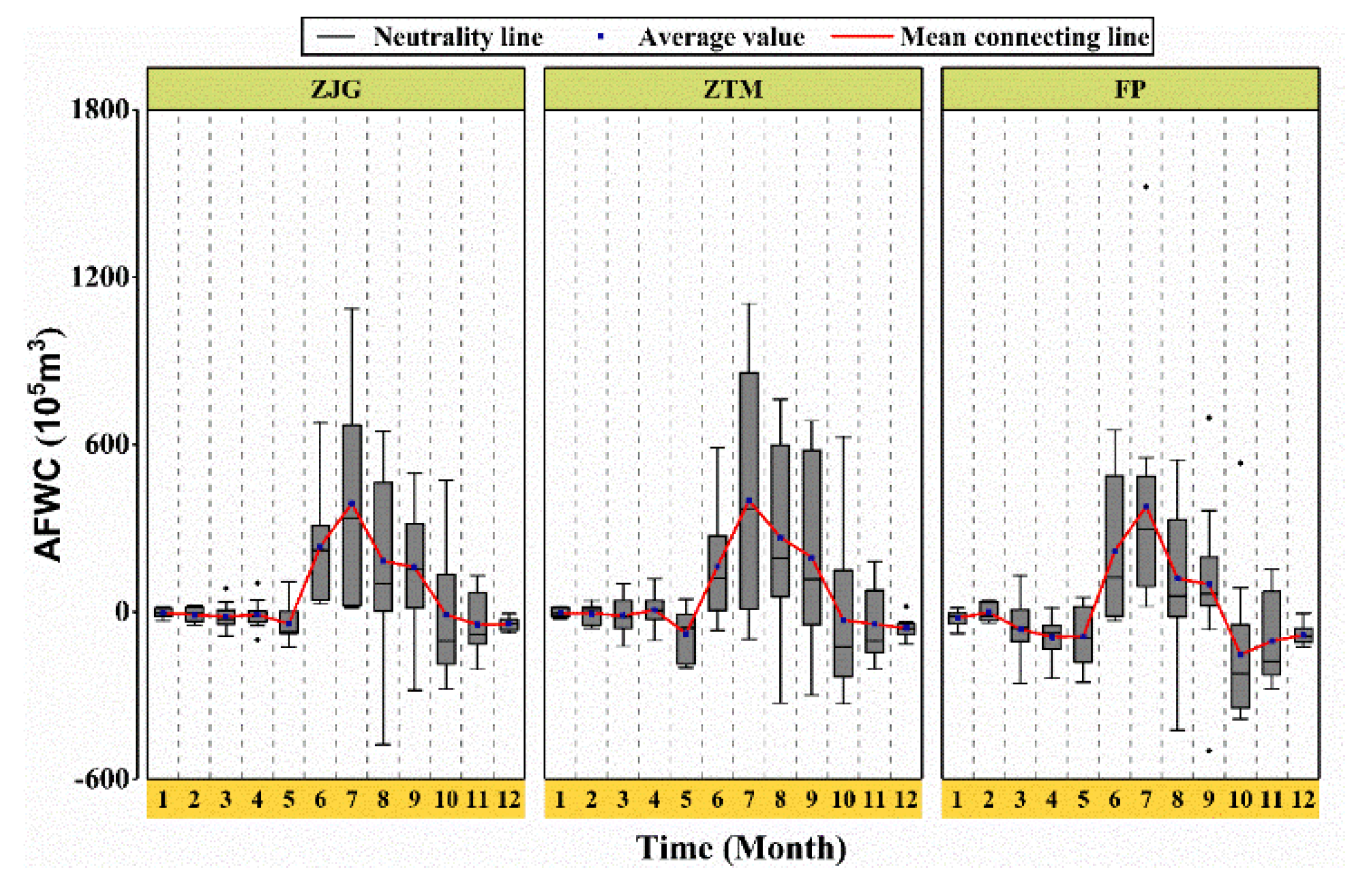
It can be seen from Figure 7 that the variation degree of AFWC in July was the largest, while the variation of AFWC in January and December was relatively small. There were large fluctuations in AFWCs between different months in each basin of the study area (Figure 7). The average AFWC of the ZJG, ZTM and FP basins reached the maximum in July, with values of 388.50, 399.34 and 377.75 (10⁵ m³), respectively. The average AFWC of the ZJG, ZTM and FP basins reached the minimum in November, May and October, with values of −45.99, −78.00 and −153.20 (10⁵ m³), respectively. The positive–negative conversion of AFWC between rainy and dry months reflects that the runoff regulation function of forest water conservation was reflected on a monthly scale.

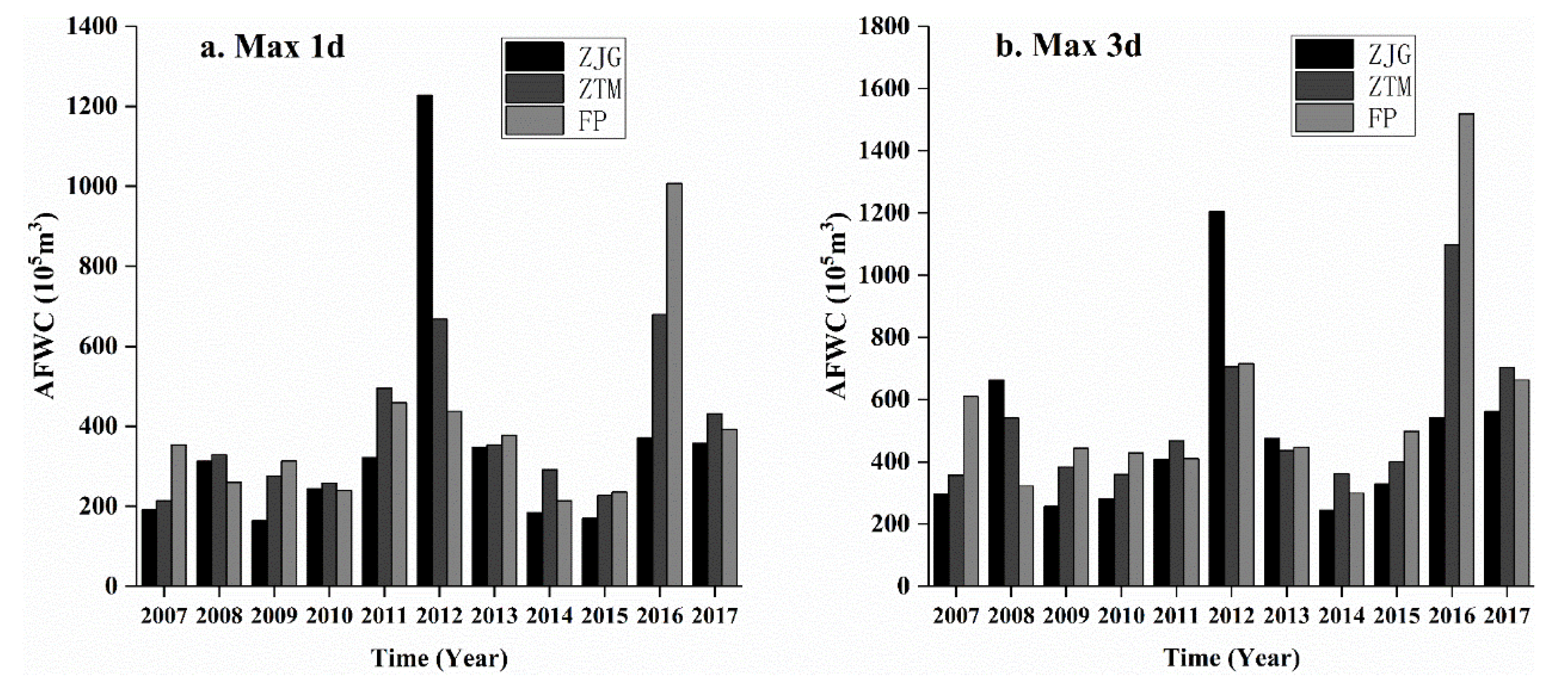
3.3.3. Daily Conservation Amount

In the ZJG, ZTM and FP basins, the AFWC of the maximum one day in a year (Max 1d) was positive (Figure 8). The minimum value of AFWC in the ZJG, ZTM and FP basins was 163.09 (10⁵ m³) in 2009, 213.97 (10⁵ m³) in 2007 and 213.06 (10⁵ m³) in 2014, respectively. The maximum value was 1227.65 (10⁵ m³) in 2012, 679.11 (10⁵ m³) in 2016 and 1006.59 (10⁵ m³) in 2016, respectively.

The minimum value of the AFWC of annual continuous maximum three days (Max 3d) in the ZJG, ZTM and FP basins was 244.56 (10⁵ m³) in 2014, 357.30 (10⁵ m³) in 2007 and 299.16 (10⁵ m³) in 2014, respectively. The maximum was 1204.79 (10⁵ m³) in 2012, 1098.31 (10⁵ m³) in 2016 and 1518.57 (10⁵ m³) in 2016, respectively (Figure 8). From the above results, it can be seen that forests play a water conservation function to intercept floods during periods of extreme precipitation.

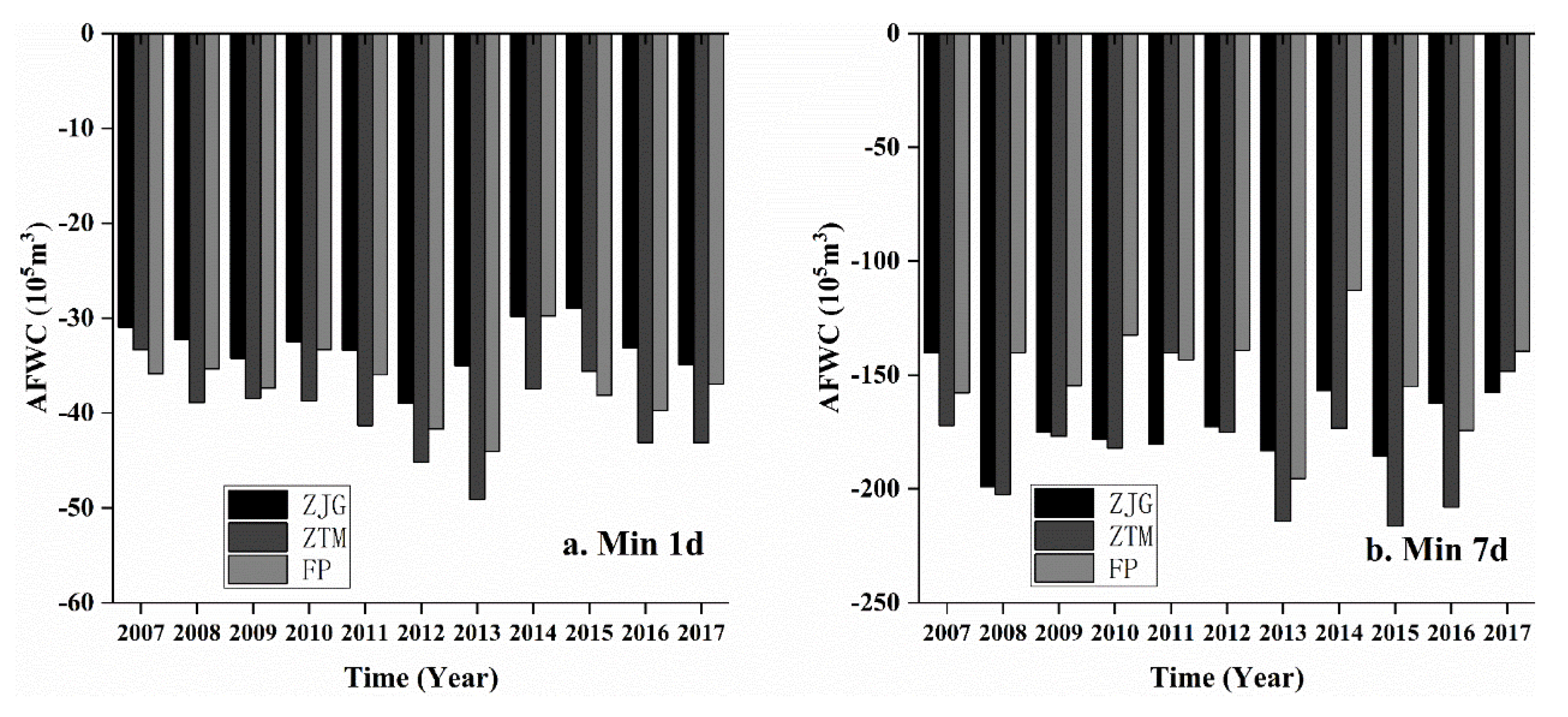
In the ZJG, ZTM and FP basins, the AFWC of the minimum one day in a year (Min 1d) was negative, indicating the loss of forest water conservation amount (Figure 9). The minimum value of AFWC loss in the ZJG, ZTM and FP basins was 28.96 (10⁵ m³) in 2015, 33.32 (10⁵ m³) in 2007 and 29.78 (10⁵ m³) in 2014, respectively; the maximum value of the loss was 38.98 (10⁵ m³) in 2012, 49.11 (10⁵ m³) in 2013 and 44.06 (10⁵ m³) in 2013, respectively.

The AFWC of annual continuous minimum seven days (Min 7d) in the ZJG basin, ZTM basin and FP basin was also negative (Figure 9). The minimum value of AFWC loss in ZJG, ZTM and FP basins was 140.21 (10⁵ m³) in 2007, 140.16 (10⁵ m³) in 2011 and 112.87 (10⁵ m³) in 2014, respectively; the maximum value of the loss was 199.03 (10⁵ m³) in 2008, 216.44 (10⁵ m³) in 2015 and 195.46 (10⁵ m³) in 2013, respectively.

4. Discussion

4.1. The Influence of the Area Threshold of Hydrological Response Unit (HRU) on the Generalization of the Land-Use Area

In the existing SWAT model application research, the area threshold of land use, soil and slope was generally selected as 5%–15% [59,60,61,62]. However, different HRU division methods will directly affect the generalized results of various land use areas generated by the SWAT model [38,63].

Table 7. Area comparison of land use HRU in the ZJG basin under different threshold conditions.

Threshold	Area of HRU under Different Land Use (km2)						Number of HRU
	Arable Land	Forest Land	Grassland	Waters	Construction Land	Bare Land
T000000	349.97	728.31	590.95	19.16	54.30	1.62	702
T011010	353.01	734.47	596.18	15.35	45.29	0.00	251
T051010	370.18	756.23	615.01	0.36	2.54	0.00	184
T101010	355.23	764.39	623.53	0.36	0.80	0.00	176
T102010	355.23	764.39	623.53	0.36	0.80	0.00	105
T102020	355.23	764.39	623.53	0.36	0.80	0.00	86

,

Table 8. Area comparison of land use HRU in the ZTM basin under different threshold conditions.

Threshold	Area of HRU Under Different Land Use (km2)						Number of HRU
	Arable Land	Forest Land	Grassland	Waters	Construction Land	Bare Land
T000000	682.79	883.65	1704.57	56.07	67.62	0.00	1572
T011010	686.98	887.90	1712.81	52.70	54.32	0.00	576
T051010	679.90	913.57	1779.09	0.58	21.57	0.00	431
T101010	622.70	937.57	1826.80	0.00	7.64	0.00	385
T102010	622.70	937.57	1826.80	0.00	7.64	0.00	226
T102020	622.70	937.57	1826.80	0.00	7.64	0.00	181

and

Table 9. Area comparison of land use HRU in the FP basin under different threshold conditions.

Threshold	Area of HRU under Different Land Use (km2)						Number of HRU
	Arable Land	Forest Land	Grassland	Waters	Construction Land	Bare Land
T000000	97.98	844.79	1160.22	22.77	22.71	0.07	829
T011010	96.89	851.68	1168.81	17.08	14.09	0.00	303
T051010	88.23	871.35	1188.23	0.70	0.03	0.00	210
T101010	3.04	900.67	1244.10	0.70	0.03	0.00	175
T102010	3.04	900.67	1244.10	0.70	0.03	0.00	112
T102020	3.04	900.67	1244.10	0.70	0.03	0.00	79

were the comparison between the HRU of land use area generated by different area thresholds (e.g., T012020 indicates that the area thresholds for land use, soil and aspect were 1%, 20% and 20%, respectively) and the actual land use area under the land use conditions in 2010. It can be seen that with the increase of area threshold, the HRU area of land use (forest land and grassland) with a larger area in the three basins increased gradually, while the HRU area of land use (waters, construction land and bare land) with relatively small area proportion decreased gradually. When the area threshold is greater than or equal to 10%, the generalized area of land use HRU will no longer change, which is in line with other studies carried out in the humid areas of South China [38].

As the area threshold increases, the number of HRUs in the three basins continues to decrease, which increases the area covered by a single HRU. In order to make the same HRU have the same land use type, soil type and slope, the land use type with the small area will be absorbed by the land use type with a large area, resulting in the area of land use type with large area proportion increasing continuously, while the area of land use type with small area proportion continues to decrease, even become 0 [64]. Therefore, the area threshold value of 0% was selected in this paper to guarantee the model could accurately reflect the spatial distribution of various land use types including forests, and ensure the rationality of the calculation results and laying a model foundation for the calculation of forest water conservation by the SWAT model.

4.2. The Influence of Climate Characteristics on the Amounts of Forest Water Conservation (AFWCs)

At the basin scale, precipitation and evapotranspiration were the main climatic factors that affect AFWC [65]. Precipitation was the recharge water source for the basin in the monsoon region and was usually positively correlated with AFWC [66,67]. Evapotranspiration is the main form of surface water consumption, which is affected by multiple factors such as air temperature, vapor pressure, wind speed, solar radiation and underlying surface conditions [68,69]. Soil evaporation and vegetation transpiration are the main forms of basin evapotranspiration, which together consume the water stored in the basin, and the amount of evapotranspiration directly affects the AFWC [70,71,72].

The wetness index (precipitation/potential evapotranspiration) was used as an indicator to measure the dry and wet climate of a certain area and has been widely used in the study of the response of the ecological environment to climate change [73,74]. In this paper, we used the wetness index to comprehensively consider the effects of precipitation and potential evapotranspiration on AFWC on different time scales.

4.2.1. Annual Scale

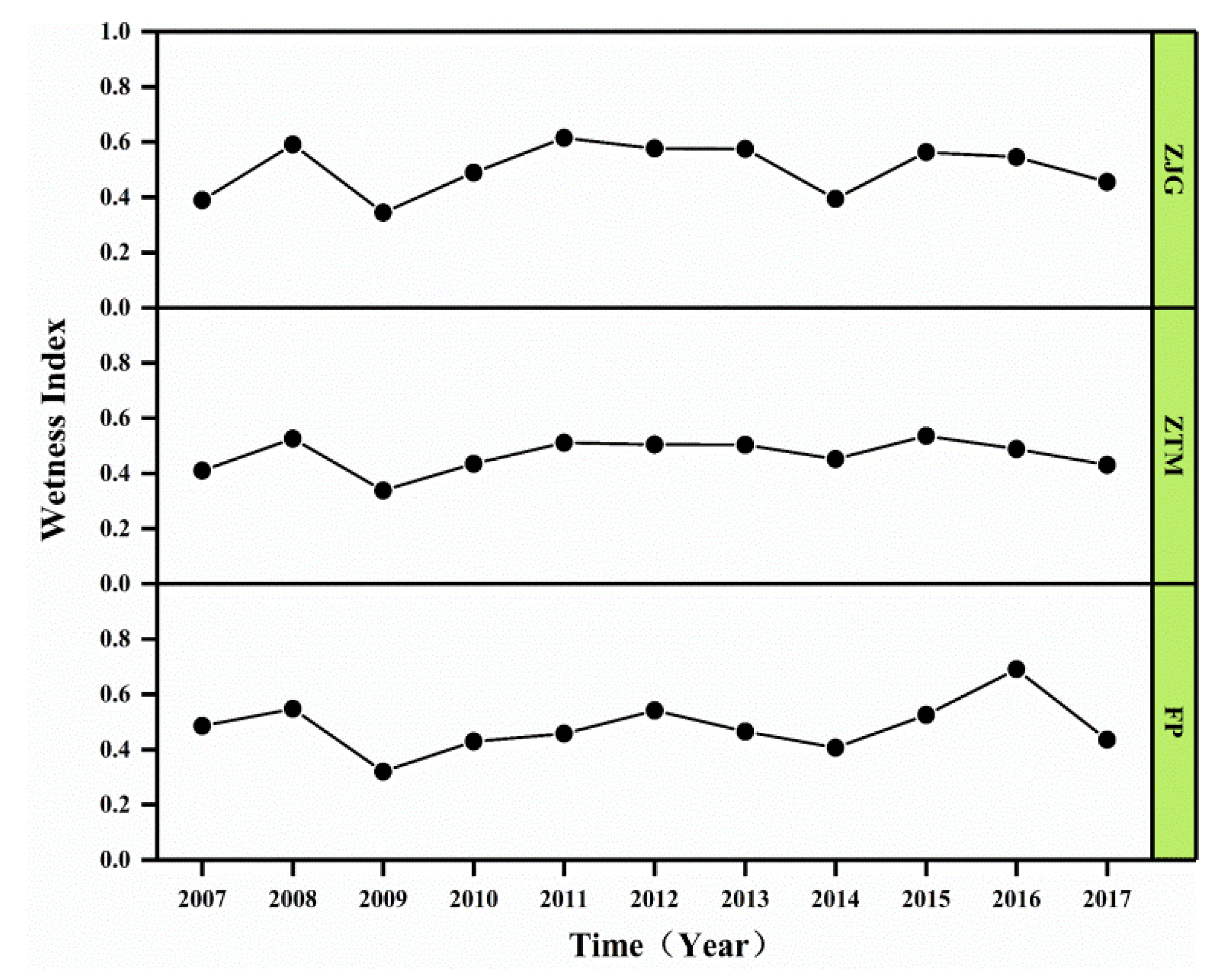
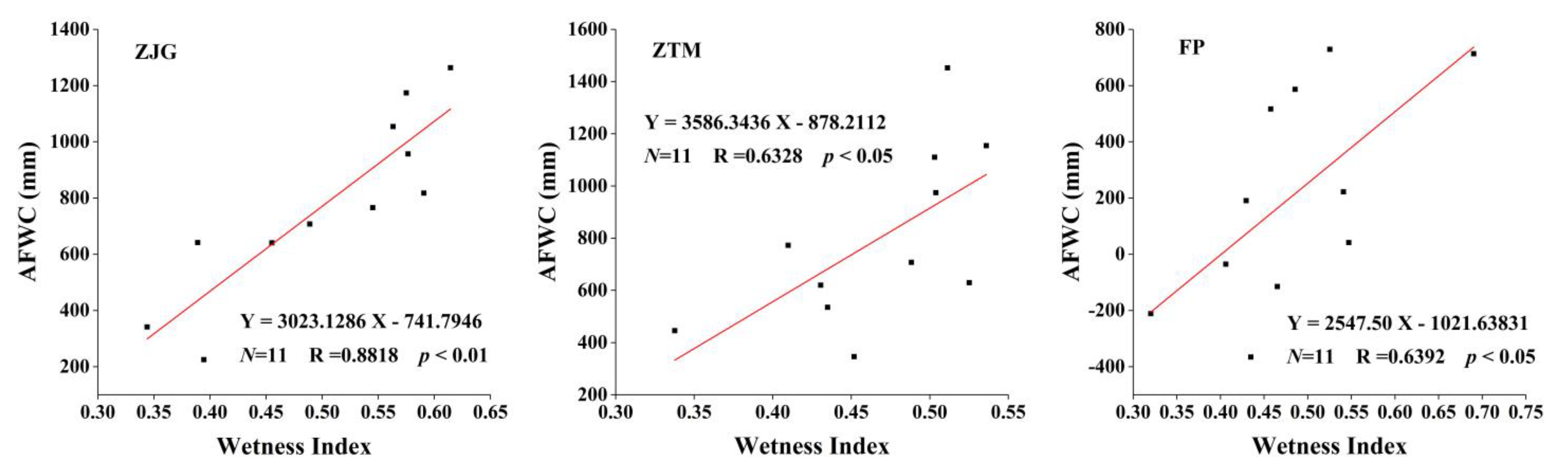
The interannual variations of the wetness indexes of the ZJG, ZTM and FP basins were small, and the multiyear average wetness index was: ZJG (0.50) > FP (0.48) > ZTM (0.47) (Figure 10). The wetness index of each basin in the study area was positively correlated with the annual AFWC (Figure 11). Among the three basins, the wetness index in the ZJG basin has the largest correlation coefficient with the annual average AFWC, which indicates that the AFWC in the ZJG basin was most affected by climate change on an annual scale. In general, the wetter the climate in the upstream of Xiong’an New Area, the greater the annual AFWC, which is in line with other studies carried out in other Chinese mountains, such as the Hengduan Mountains [75] and Qinling Mountains [76].

4.2.2. Monthly Scale

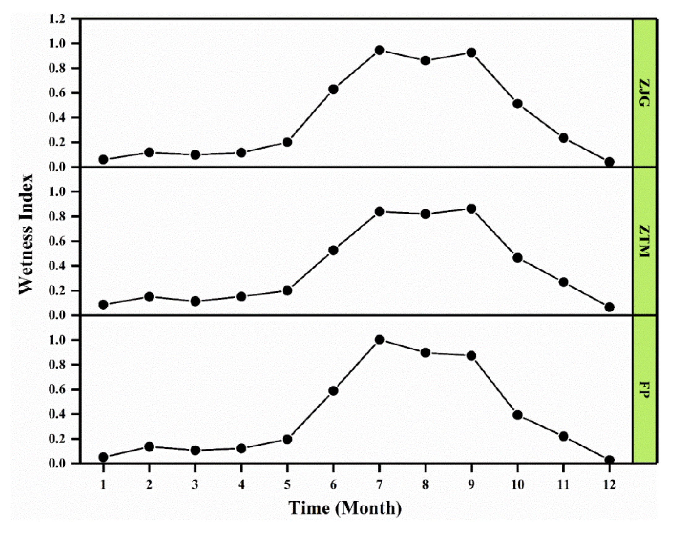
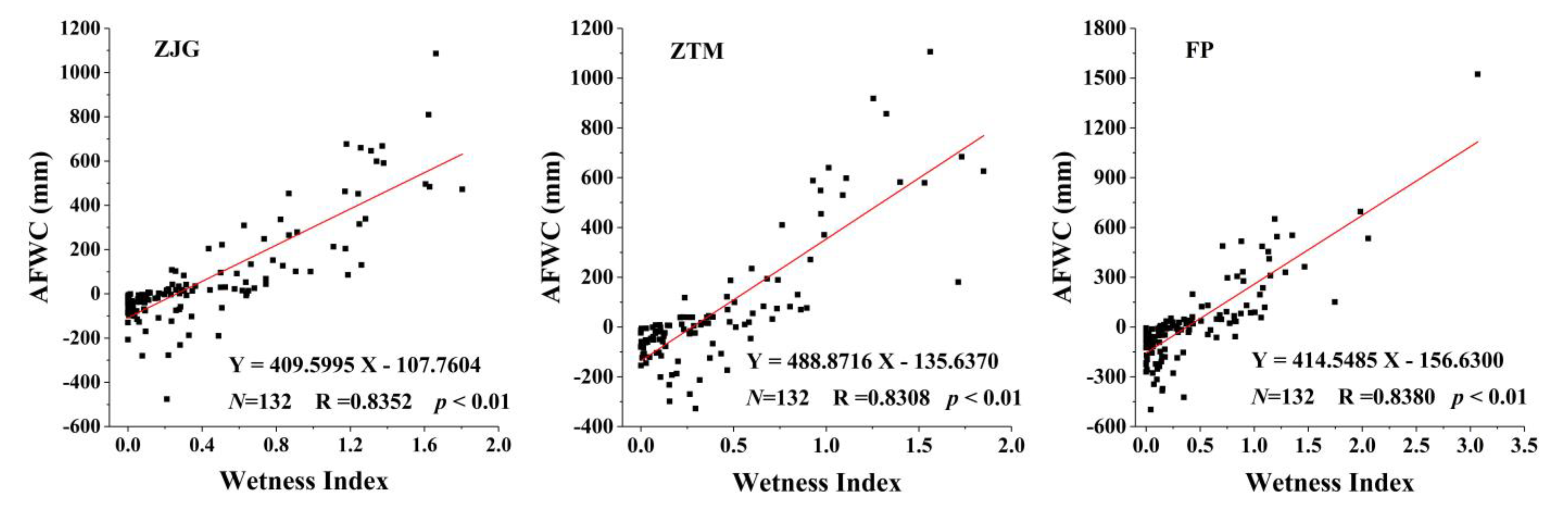
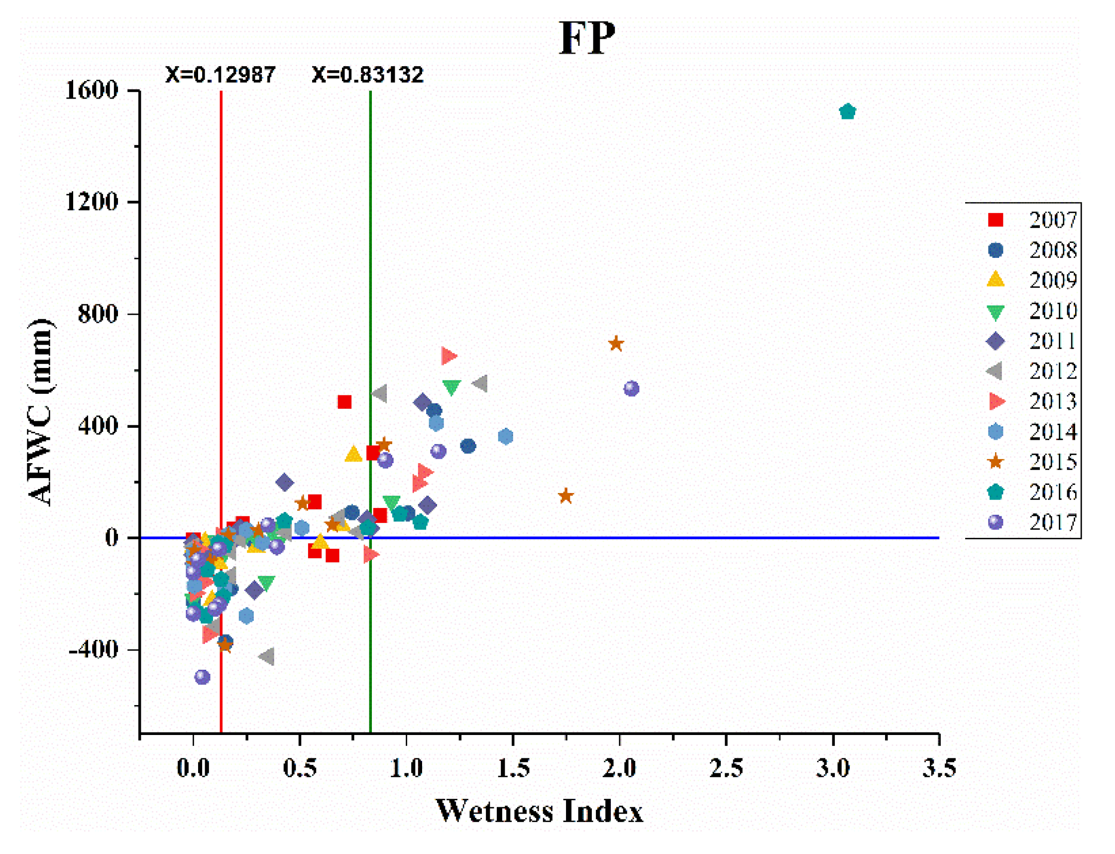
The intermonthly variation of the wetness index of the ZJG, ZTM and FP basins were large, with the average monthly wetness index being 0.40, 0.38 and 0.38, respectively (Figure 12). The months in which the wetness index of ZJG, ZTM and FP basins in the study area were higher than the average value are from June to October (Figure 12). The monthly AFWC in the ZJG ZTM and FP basins were also positively correlated with the wetness index and the correlation coefficients were all above 0.83 (p < 0.01), and the correlation was better than the annual scale (Figure 13). June to September was the most precipitation period of the year in the study area, and the climate was humid [40]. During this period, the forests fully play the function of accumulating precipitation, making AFWC significantly larger than other months. From October to May, the study area had scarce precipitation and a dry climate, which caused the water stored in the forests to be consumed for evapotranspiration and supplementary runoff [17,77], and the AFWC showed a negative value.

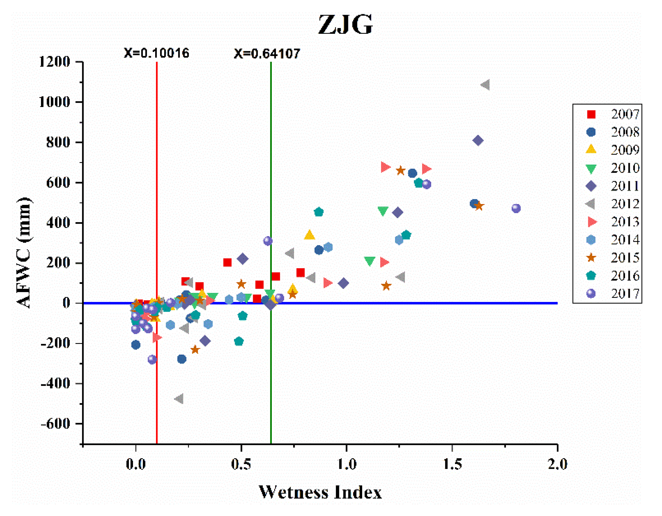
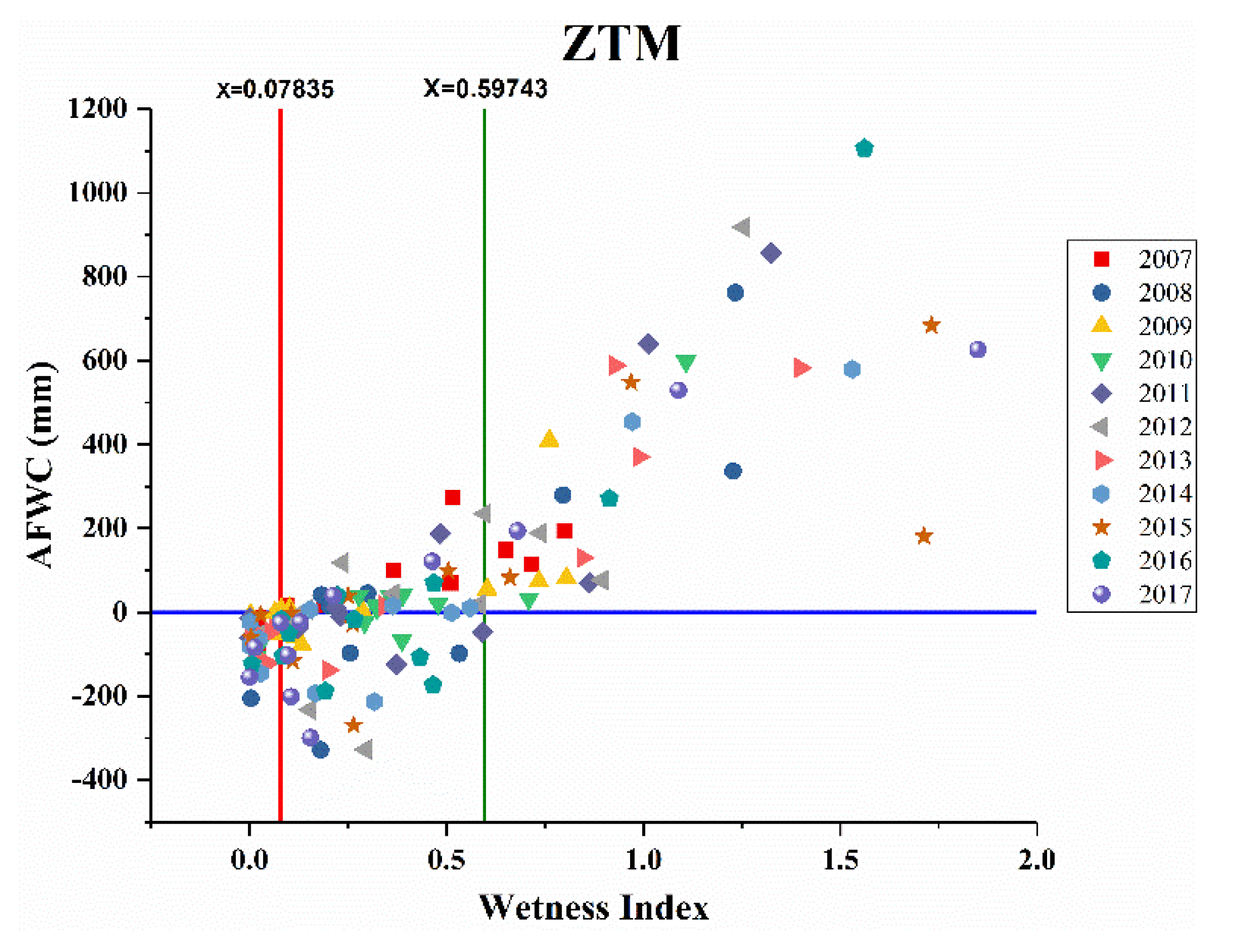
Figure 14, Figure 15 and Figure 16 are the distribution maps of monthly AFWC and wetness index in ZJG, ZTM and FP basins, respectively.

When the wetness index of the ZJG, ZTM and FP basins was greater than 0.64, 0.60 and 0.83, respectively, the AFWC in the basins was all positive. It shows that the FP basin needs more humid climate conditions than the ZJG and ZTM basins to keep the forests in a stable water storage state. When the wetness index of the ZJG, ZTM and FP basins was less than 0.10, 0.08 and 0.13, respectively, the AFWC in the basins was all negative. It indicates that the occurrence of forests water storage in the FP basin requires a more humid climate than the other two basins.

5. Conclusions

In the past, some models have been applied to the quantitative evaluation of forest water conservation functions, which only reflect the annual AFWC. However, the forest water conservation function may have different manifestations at different time scales. With the combination of the SWAT model and water balance method, a quantitative evaluation method of forest water conservation function is applied in this article. Different from the previous works, the applied method could calculate AFWC at different time scales. We present a case study in the upstream of Xiong’an New Area to study the characteristics of AFWC on annual, monthly and daily scales by applying the proposed method. The following conclusions can be drawn:

(1)

The constructed SWAT model of the three upstream basins in Xiong’an New Area has high accuracy, and the calculation formula of AFWC was suitable for the multitemporal scale analysis on AFWC in the semiarid mountains area.

(2)

On an annual scale, the forests in the ZJG and ZTM basins mainly played a role in storing precipitation. While AFWC in the FP basin was negative in 2009, 2013, 2014 and 2017, indicating the forests in this basin were in a state of water deficit during these four years. On a monthly scale, the positive values of AFWC mainly appeared in June to September, and the negative values of AFWC mainly appeared in December to March. On a daily scale, the forests played a role in flood interception during extreme precipitation, while the effect of forest water consumption during extreme droughts was obvious.

(3)

Compared with the annual AFWC, the monthly AFWC in the ZJG, ZTM and FP basins were more affected by climate change. In the three basins, the FP basin needs more humid climate conditions than the ZJG and ZTM basins to make the forests store water and keep the forests in a stable water storage state on a monthly scale.

As the most important ecological barrier area in Xiong’an New Area, the upstream of Xiong’an New Area should implement strict forest protection policies and strengthen the ability to cope with an extreme climate, to ensure the water supply and flood control safety of Xiong’an New Area.

References

- Immerzeel, W.W.; Lutz, A.F.; Andrade, M.; Bahl, A.; Biemans, H.; Bolch, T.; Hyde, S.; Brumby, S.; Davies, B.J.; Elmore, A.C.; et al. Importance and vulnerability of the world’s water towers. Nature 2020, 577, 364–369. [Google Scholar] [CrossRef] [PubMed]
- Cao, W.; Wu, D.; Huang, L.; Liu, L. Spatial and temporal variations and significance identification of ecosystem services in the Sanjiangyuan National Park, China. Sci. Rep. 2020, 10, 6151. [Google Scholar] [CrossRef] [PubMed]
- Hering, J.G.; Ingold, K.M. Water Resources Management: What Should Be Integrated? Science 2012, 336, 1234–1235. [Google Scholar] [CrossRef] [PubMed]
- Trusel, L.D.; Das, S.B.; Osman, M.B.; Evans, M.J.; Smith, B.E.; Fettweis, X.; McConnell, J.R.; Noel, B.P.Y.; van den Broeke, M.R. Nonlinear rise in Greenland runoff in response to post-industrial Arctic warming. Nature 2018, 564, 104–108. [Google Scholar] [CrossRef]
- Bloschl, G.; Kiss, A.; Viglione, A.; Barriendos, M.; Bohm, O.; Brazdil, R.; Coeur, D.; Demaree, G.; Llasat, M.C.; Macdonald, N.; et al. Current European flood-rich period exceptional compared with past 500 years. Nature 2020, 583, 560–566. [Google Scholar] [CrossRef]
- Seddon, A.W.; Macias-Fauria, M.; Long, P.R.; Benz, D.; Willis, K.J. Sensitivity of global terrestrial ecosystems to climate variability. Nature 2016, 531, 229–232. [Google Scholar] [CrossRef] [Green Version]
- Návar, J. Fitting rainfall interception models to forest ecosystems of Mexico. J. Hydrol. 2017, 548, 458–470. [Google Scholar] [CrossRef]
- Zhou, G.; Wei, X.; Luo, Y.; Zhang, M.; Li, Y.; Qiao, Y.; Liu, H.; Wang, C. Forest recovery and river discharge at the regional scale of Guangdong Province, China. Water Res. Res. 2010, 46, W09503. [Google Scholar] [CrossRef] [Green Version]
- Bonell, M.; Purandara, B.K.; Venkatesh, B.; Krishnaswamy, J.; Acharya, H.A.K.; Singh, U.V.; Jayakumar, R.; Chappell, N. The impact of forest use and reforestation on soil hydraulic conductivity in the Western Ghats of India: Implications for surface and sub-surface hydrology. J. Hydrol. 2010, 391, 47–62. [Google Scholar] [CrossRef]
- Julian, J.P.; Gardner, R.H. Land cover effects on runoff patterns in eastern Piedmont (USA) watersheds. Hydrol. Process. 2014, 28, 1525–1538. [Google Scholar] [CrossRef]
- Cao, J.; Liu, C.; Zhang, W.; Han, S. Using temperature effect on seepage variations as proxy for phenological processes of basin-scale vegetation communities. Hydrol. Process. 2013, 27, 360–366. [Google Scholar] [CrossRef]
- Fang, L.; Yi, A.; Ying, Z. The influence of silviculture investment in fixed assets on forest water conservation in China. Water Qual. Res. J. 2019, 54, 220–229. [Google Scholar]
- Kurihara, M.; Onda, Y.; Kato, H.; Loffredo, N.; Yasutaka, T.; Coppin, F. Radiocesium migration in the litter layer of different forest types in Fukushima, Japan. J. Environ. Radioact. 2018, 187, 81–89. [Google Scholar] [CrossRef] [PubMed]
- Sheng, H.; Cai, T. Influence of Rainfall on Canopy Interception in Mixed Broad-Leaved—Korean Pine Forest in Xiaoxing’an Mountains, Northeastern China. Forests 2019, 10, 248. [Google Scholar] [CrossRef] [Green Version]
- Davies-Barnard, T.; Valdes, P.J.; Jones, C.D.; Singarayer, J.S. Sensitivity of a coupled climate model to canopy interception capacity. Clim. Dyn. 2014, 42, 1715–1732. [Google Scholar] [CrossRef]
- Peng, H.; Zhao, C.; Feng, Z.; Xu, Z.; Wang, C.; Zhao, Y. Canopy interception by a spruce forest in the upper reach of Heihe River basin, Northwestern China. Hydrol. Process. 2014, 28, 1734–1741. [Google Scholar] [CrossRef]
- Liu, L.L.; Cao, W.; Shao, Q.Q. Water Conservation Function of Forest Ecosystem in the Southern and Borthern Pan River Watershed. Sci. Geogr. Sin. 2016, 36, 603–611. [Google Scholar]
- Tang, Y.Z.; Shao, Q.Q. Dataset of Water Conservation of Forest Ecosystem in the Upper Reaches of Wujiang River, China. J. Glob. Change Data Discov. 2018, 2, 433–441. [Google Scholar]
- Zhang, B.; Li, W.H.; Xie, G.D.; Xiao, Y. Water conservation function and its measurement methods of forest ecosystem. Chin. J. Ecol. 2009, 28, 529–534. [Google Scholar]
- Na, L.; Na, R.; Zhang, J.; Tong, S.; Shan, Y.; Ying, H.; Li, X.; Bao, Y. Vegetation Dynamics and Diverse Responses to Extreme Climate Events in Different Vegetation Types of Inner Mongolia. Atmosphere 2018, 9, 394. [Google Scholar] [CrossRef] [Green Version]
- Xie, H.; Kung, C.-C.; Zhao, Y. Spatial disparities of regional forest land change based on ESDA and GIS at the county level in Beijing-Tianjin-Hebei area. Front. Earth Sci. 2012, 6, 445–452. [Google Scholar] [CrossRef]
- Ding, C.; Zhang, H.; Li, X.; Li, W.; Gao, Y. Quantitative assessment of water conservation function of the natural spruce forest in the central Tianshang Mountains: A case study of the Urumqi River Basin. Acta Ecol. Sin. 2017, 37, 3733–3743. [Google Scholar]
- Zeng, L.; Li, J. A Bayesian belief network approach for mapping water conservation ecosystem service optimization region. J. Geogr. Sci. 2019, 29, 1021–1038. [Google Scholar] [CrossRef] [Green Version]
- Cong, W.; Sun, X.; Guo, H.; Shan, R. Comparison of the SWAT and InVEST models to determine hydrological ecosystem service spatial patterns, priorities and trade-offs in a complex basin. Ecol. Indic. 2020, 112, 106089. [Google Scholar] [CrossRef]
- Yang, D.; Liu, W.; Tang, L.; Chen, L.; Li, X.; Xu, X. Estimation of water provision service for monsoon catchments of South China: Applicability of the InVEST model. Landsc. Urban Plan. 2019, 182, 133–143. [Google Scholar] [CrossRef]
- Scordo, F.; Lavender, T.; Seitz, C.; Perillo, V.; Rusak, J.; Piccolo, M.; Perillo, G. Modeling Water Yield: Assessing the Role of Site and Region-Specific Attributes in Determining Model Performance of the InVEST Seasonal Water Yield Model. Water 2018, 10, 1496. [Google Scholar] [CrossRef] [Green Version]
- Xu, J.; Ji, G.; Meadows, M.E.; Chen, R.; Yang, X. Modelling water yield with the InVEST model in a data scarce region of northwest China. Water Supply 2020, 20, 1035–1045. [Google Scholar]
- Zhang, D.-D.; Yan, D.-H.; Wang, Y.-C.; Lu, F.; Liu, S.-H. GAMLSS-based nonstationary modeling of extreme precipitation in Beijing–Tianjin–Hebei region of China. Nat. Hazards 2015, 77, 1037–1053. [Google Scholar] [CrossRef]
- Lin, B.; Chen, X.; Yao, H.; Chen, Y.; Liu, M.; Gao, L.; James, A. Analyses of landuse change impacts on catchment runoff using different time indicators based on SWAT model. Ecol. Indic. 2015, 58, 55–63. [Google Scholar] [CrossRef]
- Shirazi, Z.; Guo, H.; Chen, F.; Yu, B.; Li, B. Assessing the impact of climatic parameters and their inter-annual seasonal variability on fire activity using time series satellite products in South China (2001–2014). Nat. Hazards 2016, 85, 1393–1416. [Google Scholar] [CrossRef]
- Zhang, Q.; Zeng, J.; Yue, P.; Zhang, L.; Wang, S.; Wang, R. On the land-atmosphere interaction in the summer monsoon transition zone in East Asia. Theor. Appl. Clim. 2020, 141, 1165–1180. [Google Scholar] [CrossRef]
- Tan, M.L.; Gassman, P.W.; Yang, X.; Haywood, J. A review of SWAT applications, performance and future needs for simulation of hydro-climatic extremes. Adv. Water Res. 2020, 143, 103662. [Google Scholar] [CrossRef]
- Troin, M.; Caya, D. Evaluating the SWAT’s snow hydrology over a Northern Quebec watershed. Hydrol. Process. 2014, 28, 1858–1873. [Google Scholar] [CrossRef]
- Hoang, L.; Schneiderman, E.M.; Moore, K.E.B.; Mukundan, R.; Owens, E.M.; Steenhuis, T.S. Predicting saturation-excess runoff distribution with a lumped hillslope model: SWAT-HS. Hydrol. Process. 2017, 31, 2226–2243. [Google Scholar] [CrossRef]
- Rathjens, H.; Oppelt, N. SWATgrid: An interface for setting up SWAT in a grid-based discretization scheme. Comput. Geosci. 2012, 45, 161–167. [Google Scholar] [CrossRef]
- Yang, Q.; Almendinger, J.E.; Zhang, X.; Huang, M.; Chen, X.; Leng, G.; Zhou, Y.; Zhao, K.; Asrar, G.R.; Srinivasan, R.; et al. Enhancing SWAT simulation of forest ecosystems for water resource assessment: A case study in the St. Croix River basin. Ecol. Eng. 2018, 120, 422–431. [Google Scholar] [CrossRef]
- Yang, Q.; Zhang, X.; Almendinger, J.E.; Huang, M.; Leng, G.; Zhou, Y.; Zhao, K.; Asrar, G.R.; Li, X.; Qiu, J. Improving the SWAT forest module for enhancing water resource projections: A case study in the St. Croix River Basin. Hydrol. Process. 2018, 33, 864–875. [Google Scholar] [CrossRef]
- Lin, F.; Chen, X.W.; Yao, W.Y.; Fang, Y.H.; Deng, H.J.; Wu, J.F.; Lin, B.Q. Multi-time scale analysis of water conservation in a discontinuous forest watershed based on SWAT model. Acta Geogr. Sin. 2020, 75, 1065–1078. [Google Scholar]
- Cui, H.; Xiao, W.; Zhou, Y.; Hou, B.; Lu, F.; Pei, M. Spatial and Temporal Variations in Vegetation Cover and Responses to Climatic Variables in the Daqing River Basin, North China. J. Coast. Res. 2019, 93, 450. [Google Scholar] [CrossRef]
- Zhao, G.; Zhou, H.; Liu, X.; Li, K.; Zhang, P.; Wen, W.; Yu, Y. PHAHs in 14 principal river sediments from Hai River basin, China. Sci. Total Environ. 2012, 427–428, 139–145. [Google Scholar] [CrossRef]
- Sun, C.; Ren, L. Assessment of surface water resources and evapotranspiration in the Haihe River basin of China using SWAT model. Hydrol. Process. 2013, 27, 1200–1222. [Google Scholar] [CrossRef]
- Zhang, X.; Ren, L.; Kong, X. Estimating spatiotemporal variability and sustainability of shallow groundwater in a well-irrigated plain of the Haihe River basin using SWAT model. J. Hydrol. 2016, 541, 1221–1240. [Google Scholar] [CrossRef]
- Xu, H.; Wang, M.; Shi, T.; Guan, H.; Fang, C.; Lin, Z. Prediction of ecological effects of potential population and impervious surface increases using a remote sensing based ecological index (RSEI). Ecol. Indic. 2018, 93, 730–740. [Google Scholar] [CrossRef]
- Wang, Z.; Cao, J.; Zhu, C.; Yang, H. The Impact of Land Use Change on Ecosystem Service Value in the Upstream of Xiong’an New Area. Sustainability 2020, 12, 5707. [Google Scholar] [CrossRef]
- Hu, J.; Lv, Y.H.; Zhang, K.; Tao, Y.Z.; Li, T.; Ren, Y. The differences of water conservation function under typical vegetation types in the Pailugou catchment, Qilian Mountain, northwest China. Acta Ecol. Sin. 2016, 36, 3338–3349. [Google Scholar]
- Wang, S.; Fu, B.; Gao, G.; Liu, Y.; Zhou, J. Responses of soil moisture in different land cover types to rainfall events in a re-vegetation catchment area of the Loess Plateau, China. Catena 2013, 101, 122–128. [Google Scholar] [CrossRef]
- Moriasi, D.N.; Arnold, J.G.; Van Liew, M.W.; Bingner, R.L.; Harmel, R.D.; Veith, T.L. Model evaluation guidelines for systematic quantification of accuracy in watershed simulations. Trans. ASABE 2007, 50, 885–900. [Google Scholar] [CrossRef]
- Arnold, J.G.; Srinivasan, R.; Muttiah, R.S.; Williams, J.R. Large Area Hydrologic Modeling and Assessment Part I: Model Development. J. Am. Water Res. Assoc. 1998, 34, 73–89. [Google Scholar] [CrossRef]
- Yang, J.; Reichert, P.; Abbaspour, K.C.; Xia, J.; Yang, H. Comparing uncertainty analysis techniques for a SWAT application to the Chaohe Basin in China. J. Hydrol. 2008, 358, 1–23. [Google Scholar] [CrossRef]
- Abbaspour, K.C.; Rouholahnejad, E.; Vaghefi, S.; Srinivasan, R.; Yang, H.; Kløve, B. A continental-scale hydrology and water quality model for Europe: Calibration and uncertainty of a high-resolution large-scale SWAT model. J. Hydrol. 2015, 524, 733–752. [Google Scholar] [CrossRef] [Green Version]
- Han, E.; Merwade, V.; Heathman, G.C. Implementation of surface soil moisture data assimilation with watershed scale distributed hydrological model. J. Hydrol. 2012, 416–417, 98–117. [Google Scholar] [CrossRef]
- Nash, J.E.; Sutcliffe, J.V. River flow forecasting through conceptual models part I—A discussion of principles. J. Hydrol. 1970, 10, 282–290. [Google Scholar] [CrossRef]
- Zuo, D.; Xu, Z.; Yao, W.; Jin, S.; Xiao, P.; Ran, D. Assessing the effects of changes in land use and climate on runoff and sediment yields from a watershed in the Loess Plateau of China. Sci. Total Environ. 2016, 544, 238–250. [Google Scholar] [CrossRef] [PubMed]
- Van Griensven, A.; Meixner, T.; Grunwald, S.; Bishop, T.; Diluzio, M.; Srinivasan, R. A global sensitivity analysis tool for the parameters of multi-variable catchment models. J. Hydrol. 2006, 324, 10–23. [Google Scholar] [CrossRef]
- Kang, H.; Moon, J.; Shin, Y.; Ryu, J.; Kum, D.H.; Jang, C.; Choi, J.; Kong, D.S.; Lim, K.J. Modification of SWAT auto-calibration for accurate flow estimation at all flow regimes. Paddy Water Environ. 2015, 14, 499–508. [Google Scholar] [CrossRef]
- Deng, K.; Shi, P.; Xi, G. Water conservation of forest ecosystem in the upper reaches of yangtze river and its benefits. Res. Sci. 2002, 24, 68–73. [Google Scholar]
- Nakano, H. Forest Hydrology. In Forest Hydrology; China Forestry Publishing House: Beijing, China, 1983; pp. 207–212. [Google Scholar]
- Feng, P.; Wu, J.; Li, J. Changes in flood characteristics and the flood driving mechanism in the mountainous Haihe River Basin, China. Hydrol. Sci. J. 2019, 64, 1997–2005. [Google Scholar] [CrossRef]
- Qiu, L.; Zheng, F.; Yin, R. Effects of DEM resolution and watershed subdivision on hydrological simulation in the Xingzihe watershed. Acta Ecol. Sin. 2012, 32, 3754–3763. [Google Scholar]
- Di Luzio, M.; Arnold, J.G.; Srinivasan, R. Effect of GIS data quality on small watershed stream flow and sediment simulations. Hydrol. Process. 2005, 19, 629–650. [Google Scholar] [CrossRef]
- Liang, K.; Jiang, Y.; Qi, J.; Fuller, K.; Nyiraneza, J.; Meng, F.R. Characterizing the impacts of land use on nitrate load and water yield in an agricultural watershed in Atlantic Canada. Sci. Total Environ. 2020, 729, 138793. [Google Scholar] [CrossRef]
- Patil, A.; Ramsankaran, R. Improving streamflow simulations and forecasting performance of SWAT model by assimilating remotely sensed soil moisture observations. J. Hydrol. 2017, 555, 683–696. [Google Scholar] [CrossRef]
- Jha, M.; Gassman, P.W.; Secchi, S.; Gu, R.; Arnold, J. Effect of watershed subdivision on swat flow, sediment, and nutrient predictions. J. Am. Water Res. Assoc. 2004, 40, 811–825. [Google Scholar] [CrossRef] [Green Version]
- Her, Y.; Frankenberger, J.; Chaubey, I.; Srinivasan, R. Threshold Effects in HRU Definition ofthe Soil and Water Assessment Tool. Trans. ASABE 2015, 58, 367–378. [Google Scholar]
- Tang, Y.; Tang, Q.; Wang, Z.; Chiew, F.H.S.; Zhang, X.; Xiao, H. Different Precipitation Elasticity of Runoff for Precipitation Increase and Decrease at Watershed Scale. J. Geophysic. Res. Atmos. 2019, 124, 11932–11943. [Google Scholar] [CrossRef]
- Zhang, F.; Li, X.; Feng, Q.; Wang, H.; Wei, Y.; Bai, H. Spatial and temporal variation of water conservation in the upper reaches of Heihe River basin based on InVEST model. J. Desert Res. 2018, 38, 1321–1329. [Google Scholar]
- Song, S.; Li, L.; Chen, X.; Bai, J. The dominant role of heavy precipitation in precipitation change despite opposite trends in west and east of northern China. Int. J. Clim. 2015, 35, 4329–4336. [Google Scholar] [CrossRef]
- Maček, U.; Bezak, N.; Šraj, M. Reference evapotranspiration changes in Slovenia, Europe. Agric. For. Meteorol. 2018, 260-261, 183–192. [Google Scholar] [CrossRef]
- Liu, L.; Wang, Z.; Wang, Y.; Zhang, Y.; Shen, J.; Qin, D.; Li, S. Trade-off analyses of multiple mountain ecosystem services along elevation, vegetation cover and precipitation gradients: A case study in the Taihang Mountains. Ecol. Indic. 2019, 103, 94–104. [Google Scholar] [CrossRef]
- Li, X.; Li, Y.; Zhang, Q.; Xu, X. Evaluating the influence of water table depth on transpiration of two vegetation communities in a lake floodplain wetland. Hydrol. Res. 2016, 47, 293–312. [Google Scholar] [CrossRef] [Green Version]
- Heitman, J.L.; Horton, R.; Sauer, T.J.; DeSutter, T.M. Sensible Heat Observations Reveal Soil-Water Evaporation Dynamics. J. Hydrometeorol. 2008, 9, 165–171. [Google Scholar] [CrossRef] [Green Version]
- Uddin, J.; Foley, J.P.; Smith, R.J.; Hancock, N.H. A new approach to estimate canopy evaporation and canopy interception capacity from evapotranspiration and sap flow measurements during and following wetting. Hydrol. Process. 2016, 30, 1757–1767. [Google Scholar] [CrossRef]
- Gavilán, P.; Castillo-Llanque, F. Estimating reference evapotranspiration with atmometers in a semiarid environment. Agric. Water Manag. 2009, 96, 465–472. [Google Scholar] [CrossRef]
- Zhou, G.; Wei, X.; Chen, X.; Zhou, P.; Liu, X.; Xiao, Y.; Sun, G.; Scott, D.F.; Zhou, S.; Han, L.; et al. Global pattern for the effect of climate and land cover on water yield. Nat. Commun. 2015, 6, 5918. [Google Scholar] [CrossRef] [PubMed] [Green Version]
- Hong, Y.; Yu, S.; Yang, X.; Luo, Y. Study on Spatial—Temporal Changes and Driving Factors of Water Conservation in Hengduan Mountain Region. Geomat. Spat. Inf. Technol. 2019, 42, 72–76. [Google Scholar]
- Ning, Y.; Zhang, F.; Feng, Q.; Wei, Y.; Ding, J.; Zhang, Y. Temporal and spatial variation of water conservation function in Qinling Mountain and its influencing factors. Chin. J. Ecol. 2020, 39, 3080–3091. [Google Scholar]
- Wang, X.; Shen, H.; Li, X.; Jing, F. Concepts, processes and quantification methods of the forest water conservation at the multiple scales. Acta Ecol. Sin. 2013, 33, 1019–1030. [Google Scholar] [CrossRef]
Figure 1.
Locations of the study area and hydrological gauging stations (coordinates system: D_WGS_1984) (basins are shown by abbreviated names: ZJG—Zijingguan; ZTM—Zhongtangmei and FP—Fuping).
Figure 2.
Simulation process of hydrological response units (HRUs) in the soil and water assessment tool (SWAT) model.
Figure 3.
The hydrological process of HRU in the SWAT model.
Figure 4.
(a) Spatial distribution of forest HRUs divided by the SWAT model and (b) spatial distribution of actual forest patches.
Figure 5.
Interannual values of amount of forest water conservation (AFWC) and precipitation.
Figure 6.
The AFWC in each month from 2007 to 2017.
Figure 7.
Changes in the average value of AFWC for each month from 2007 to 2017.
Figure 8.
(a) The AFWC of the maximum one day in a year and (b) The AFWC of annual continuous maximum three days.
Figure 9.
(a) The AFWC of the minimum one day in a year and (b) The AFWC of annual continuous minimum seven days.
Figure 10.
Interannual values of the wetness index.
Figure 11.
The correlation between AFWC and the wetness index on an annual scale.
Figure 12.
Monthly variability of the wetness index.
Figure 13.
The correlation between AFWC and the wetness index on a monthly scale.
Figure 14.
Distribution map of monthly AFWC and the wetness index in the ZJG basin from 2007 to 2017 (red line—marks the wetness index maximum value that limits the negative AFWC area and green line—marks the wetness index minimum value that limits the positive AFWC area).
Figure 15.
Distribution map of monthly AFWC and the wetness index in the ZTM basin from 2007 to 2017 (red line—marks the wetness index maximum value that limits the negative AFWC area and green line—marks the wetness index minimum value that limits the positive AFWC area).
Figure 16.
Distribution map of monthly AFWC and the wetness index in the FP basin from 2007 to 2017 (red line—marks the wetness index maximum value that limits the negative AFWC area and green line—marks the wetness index minimum value that limits the positive AFWC area).