Article

IoT Monitoring of Urban Tree Ecosystem Services: Possibilities and Challenges

1
Department of Landscape Design and Sustainable Ecosystems, Agrarian-Technological Institute, RUDN University, Miklukho-Maklaya str., 6, 117198 Moscow, Russia
2
Department of Sustainable Agro-ecosystems and Bioresources, Research and Innovation Centre, Fondazione Edmund Mach, Via E. Mach, 1 38010 San Michele all’Adige, Italy
3
Department of ecology, Russian Timiryazev State Agrarian University, Timiryazevskaya st., 49, 127550 Moscow, Russia
4
Department of Agricultural, Food and Forestry Sciences, University of Palermo, Viale delle Scienze, Ed. 4, 90128 Palermo, Italy
5
Department of Environmental, Biological and Pharmaceutical Sciences and Technologies, Campania University “Luigi Vanvitelli”, Via Vivaldi 43, 81100 Caserta, Italy
6
Department for Innovation in Biological, Agro-Food and Forest Systems, University of Tuscia, Via S.M. in Gradi n.4, 01100 Viterbo, Italy
7
CMCC Foundation, via Augusto Imperatore, 16, 73100 Lecce, Italy
*
Author to whom correspondence should be addressed.
Forests 2020, 11(7), 775; https://doi.org/10.3390/f11070775
Submission received: 28 May 2020 / Revised: 16 July 2020 / Accepted: 17 July 2020 / Published: 19 July 2020
(This article belongs to the Special Issue Assessing, Valuing and Mapping Ecosystem Services)

Abstract

:
Urban green infrastructure plays an increasingly significant role in sustainable urban development planning as it provides important regulating and cultural ecosystem services. Monitoring of such dynamic and complex systems requires technological solutions which provide easy data collection, processing, and utilization at affordable costs. To meet these challenges a pilot study was conducted using a network of wireless, low cost, and multiparameter monitoring devices, which operate using Internet of Things (IoT) technology, to provide real-time monitoring of regulatory ecosystem services in the form of meaningful indicators for both human health and environmental policies. The pilot study was set in a green area situated in the center of Moscow, which is exposed to the heat island effect as well as high levels of anthropogenic pressure. Sixteen IoT devices were installed on individual trees to monitor their ecophysiological parameters from 1 July to 31 November 2019 with a time resolution of 1.5 h. These parameters were used as input variables to quantify indicators of ecosystem services related to climate, air quality, and water regulation. Our results showed that the average tree in the study area during the investigated period reduced extreme heat by 2 °C via shading, cooled the surrounding area by transferring 2167 ± 181 KWh of incoming solar energy into latent heat, transpired 137 ± 49 mm of water, sequestered 8.61 ± 1.25 kg of atmospheric carbon, and removed 5.3 ± 0.8 kg of particulate matter (PM10). The values of the monitored processes varied spatially and temporally when considering different tree species (up to five to ten times), local environmental conditions, and seasonal weather. Thus, it is important to use real-time monitoring data to deepen understandings of the processes of urban forests. There is a new opportunity of applying IoT technology not only to measure trees functionality through fluxes of water and carbon, but also to establish a smart urban green infrastructure operational system for management.

1. Introduction

Urbanization is increasing on a global scale, with more than half of the world′s population presently living in cities, with expectations for cities to reach two-thirds of the world population by 2050 [1]. This shift is driven by positive factors like economic opportunities and higher levels of innovation and technology [2]. That said, in most cases, urban development and population concentration do not follow sustainability criteria, resulting in growing health risks [3,4]. Additionally, energy-intensive systems significantly contribute to global carbon emissions, ecosystem degradation, and biodiversity loss on a global scale [5,6]. It is well-known that urban ecosystems are heterotrophic ecosystems depending on natural capital and provisions from the ecosystem services (ES) of extra-urban areas [7,8,9]. Conversely, the role of ecosystem services within the boundaries of the urban areas is still open to investigation to clarify many aspects of uncertainty and to identify the most representative ecological functions that describe meaningful ecosystem services for different purposes [10,11,12,13,14]. Among the different ES, regulatory and cultural services are the most important for scientific and policy initiatives related to green infrastructure in urban areas [15,16].
Urban green infrastructure (UGI), and trees in particular, play an essential role in the sustainable functioning of urban ecosystems and provide regulating and habitat ES such as carbon sequestration, microclimate formation, pollution and dust reduction in atmospheric air, water balance control, wildlife habitat, and wind and noise reduction [11,12,15]. The magnitude of the ES provided depends on the characteristics of UGI, such as vegetation type, age, structure, and management practices, which are important for comparison with natural ecosystems [10,17,18,19]. For the ES assessment the importance of developing appropriate indicators has been recognized [16,20] and many ES indicators have been developed, applied, tested, and reviewed [11,21,22]. ES indicators need to be relevant to a specific purpose (e.g., to reflect difference in land management—[19]) or components (e.g., soils—[23,24]) or spatial–temporal scale [25,26] to avoid uncertainties from that side, but at the same time ES indicators should inform decision-making [20,27,28]. It is clear for decision-makers that you cannot manage what you do not measure, thus these indicators should be linked to measurable policy targets and should help to monitor policy progress.
Although the concept of “ecosystem service” has made it much easier for citizens, policymakers, and urban planners to understand the advantages offered by green urban infrastructure, several limits to the operational definition and quantification of such entities still remain [24,29]. This issue is particularly true for regulatory services for which it is necessary to identify and quantify a functional relationship between specific features of green infrastructure and environmental variables increasing human well-being and sustainability. This requires optimal technical solutions which are “user friendly,” meaning that they can be offered to non-scientific operators and municipal decision-makers, in the form of continuous and real-time data which can be collected and managed with minimal effort by the users. An additional relevant aspect of the economic feasibility of large-scale monitoring systems is the wide distribution of measuring stations that might be necessary to cover the complex spatial variability of the city [14].
The fast-growing fields of information and communication technologies (ICTs) and IoT tools provide new ways to wire nature into “smart” monitoring systems. Smart technologies have been used in many environmental management efforts, such as mapping changes in vegetation composition and structure [30], managing forest regeneration with precision farming [31], running and regulating at-distance greenhouse systems with wireless sensor networks [32,33], and monitoring urban noise pollution with acoustic sensors [34,35].
This work presents the results of a pilot study which was conducted in a green area situated in the center of Moscow using a network of wireless, low cost, and multiparameter monitoring devices TreeTalkers (TT+) [36], to monitor single-tree ecophysiological parameters. This study aimed at testing the feasibility of the proposed technological solution to provide real-time monitoring of regulatory ecosystem services, reported in the form of meaningful indicators for potential end-users and relevant for both human health and environmental policy targets. This is particularly relevant since the New Moscow Development Project, adopted in 2012, is continuing to expand UGI as result of active urbanization on an area of more than 1500 km2, the impact of which on soils and ecosystems services is already visible [37]. As such, its monitoring and operational management is greatly required.

2. Materials and Methods

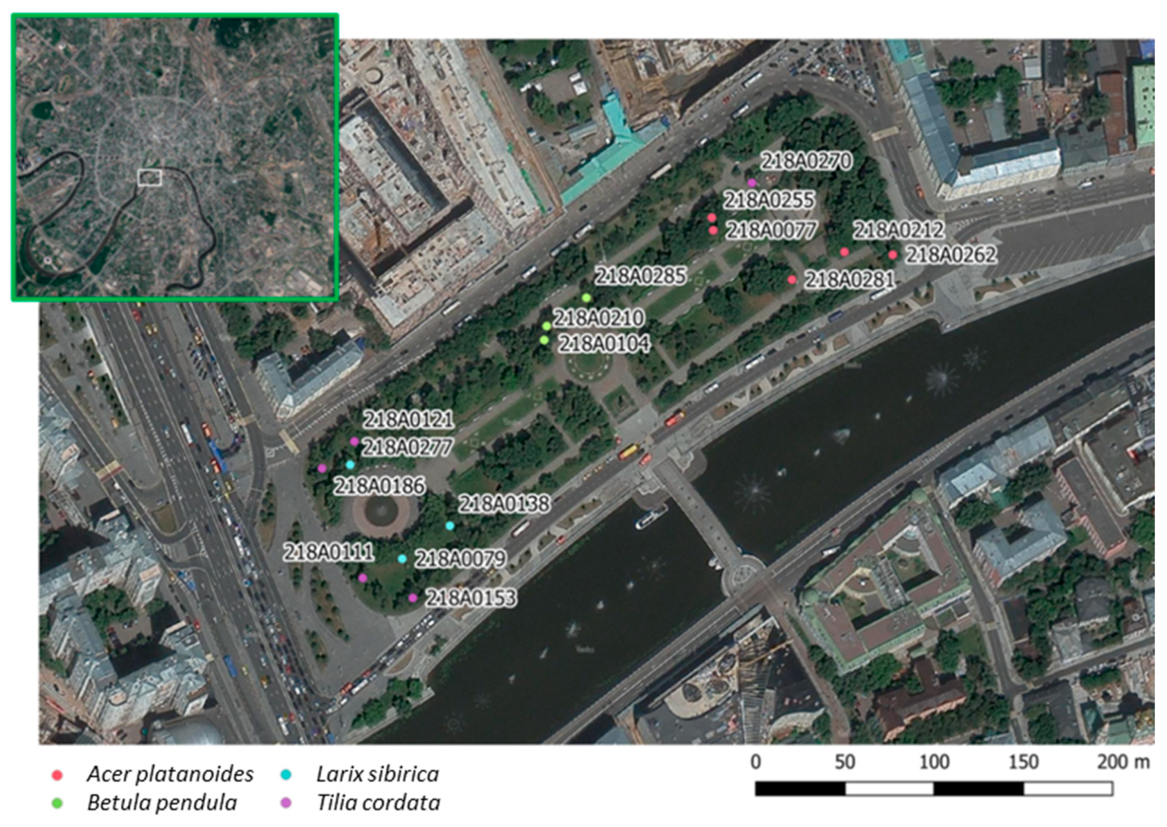
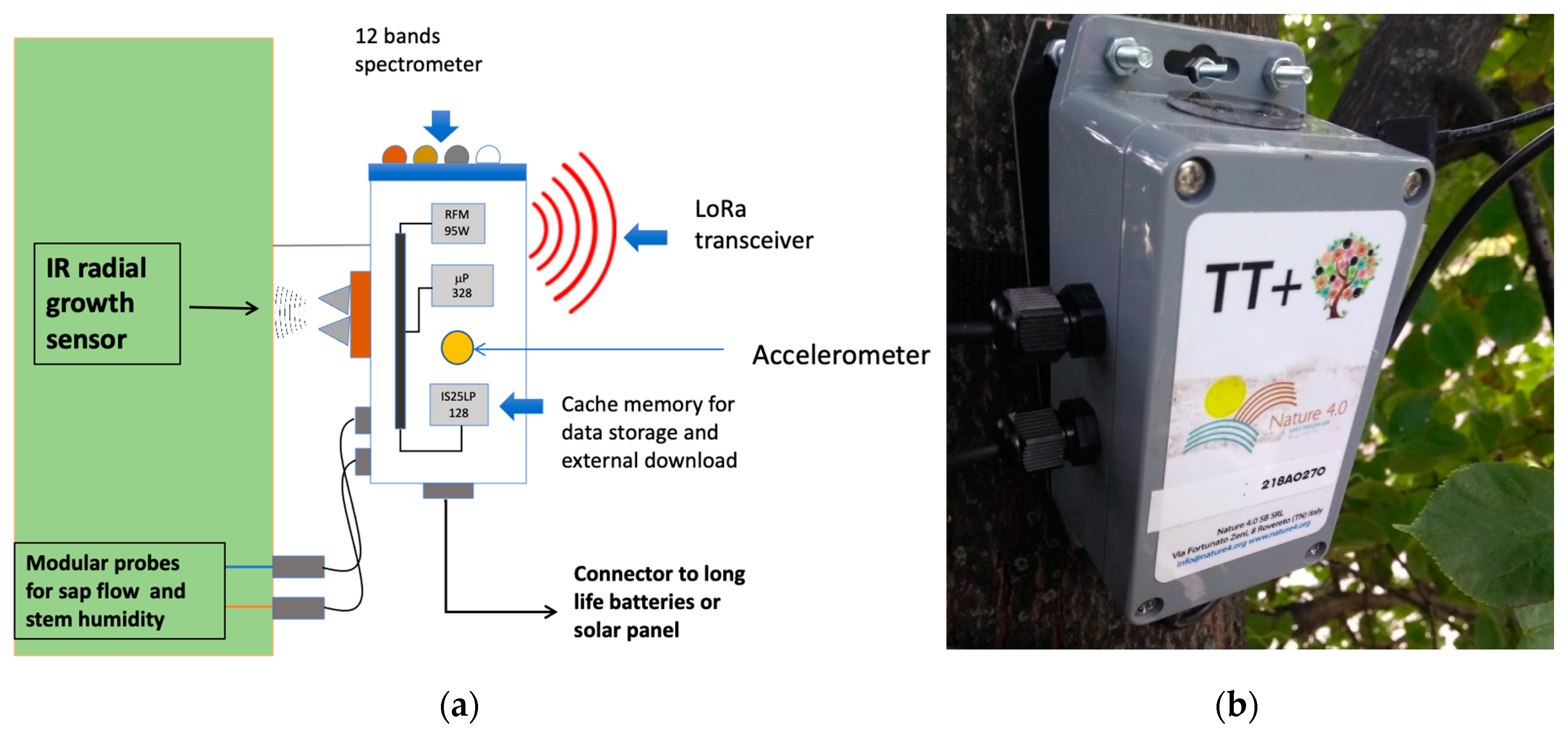
2.1. Study Site and Network Setup

With a population of over 12 million people, Moscow is the largest metropolis in Europe. The urban vegetation is made of species characteristic of the south taiga zone [38], mainly conserved in urban parks. It also includes introduced genera such as Tilia, Acer, Salix, and other ornamental forms of trees and shrubs. According to the Köppen climate classification, the climate in this area is a humid continental climate. The study site is a greened public place (green area) created in 1948, located in the Bolotnaya square in central Moscow 600 m to the south of the Kremlin, on Balchug Island. The area is under the higher influence of urban heat (mean annual air temperature is +1.8 °C than the rural reference—[39,40]) with a high level of anthropogenic pressure. The area covers about 4.5 hectares (Figure 1).
The nearby Balchug meteorological station (700 meters distance) provided meteorological data at a 3 h frequency. The daily mean temperature varied between −6.7 °C in February and +19.2 °C in July, and the amount of precipitation was about 700 mm/year, mainly in the summer months.
TreeTalker+ devices (TT+) are microprocessor-based IoT platforms built around the ATMEGA328p (Atmel Corp) chip, equipped with a LoRa transceiver for radio transmission to a central gateway, which collects the individual tree data and send it to the cloud using GSM/GPRS technology. The TT+ were first developed and tested by our team [36,41,42] and later, based on our design, industrialized by the Nature4 Benefit Corporation (www.nature4.org) based in Italy, which is a start-up company dedicated to environmental monitoring. The TT+ sensors are able to measure (1) the sap-flow density, using the transient thermal dissipation method based on a heating/cooling cycle of 10 min every 1.5 h [43]; (2) the light transmission spectra through the canopy in 12 spectral bands, using two spectrometers (VIS and NIR); (3) diameter growth with an optical IR-pulsed device; and (4) stem position and oscillation in three axes with an on-board accelerometer. In addition, air temperature and humidity are recorded at the single-tree level. Specifications and pictures are listed in Table 1 and Figure 2, respectively.
Sixteen TreeTalker+ (TT+) devices were installed on corresponding trees of four different tree species, five on Acer platanoides (average diameter at breast height (DBH) 38.7 cm), three on Betula pendula (average DBH 21.8 cm), three on Larix sibirica (average DBH 32.1 cm), and five on Tilia cordata (average DBH 34.1 cm). At the onset of installation, all trees were characterized by height, diameter, age, standing type (on the edge of the square or inside it), and VTA (visual tree assessment) [44]. The investigated trees’ VTA scores ranged from 1 to 3; from a scale of 1 (healthy condition) to 7 (severe decline), (see Appendix A). A reference device TT+ (TT-R) was mounted outside of the tree canopies to collect climate data and incoming solar radiation reference spectra. On individual trees, the devices were placed at a height of 3 m from the ground on the north side of the trunk, and the solar-powered batteries, on the south side. The 3 m height was chosen to reduce the risk of damage or theft of devices. All measurements were conducted from 01 July till 31 November 2019 with 1.5 h temporal resolution.

2.2. Choice of ES Indicators

A wide range of existing ES indicators have been investigated in previous studies [11,45]. For the present study, the ES indicators were chosen on the basis of the possibility to be directly estimated by our measured parameters. The ES indicators and the relative measured variables, including algorithm references are shown on Table 2. Direct measurements (like air temperature or relative humidity) gave us an opportunity to calculate ESI without any additional assumptions. However, all the ESI that are labeled as “indirect” required us to introduce some adjustment factors or assumptions. One of the most frequently-used “indirect” predictors of ES is tree leaf area index (LAI) since many ESI can be estimated by the amount of leaf area [11,45]. For the purpose of this paper we monitored LAI in real-time by using the two on-board spectrometers and we present particulate adsorption (calculated based on iTree model’s equations [46]) as an example of usefulness of LAI indicator indirect use.

2.2.1. Carbon Sequestration

Carbon sequestration assessment was based on the Intergovernmental Panel on Climate Change (IPCC) approach [69], utilizing biomass expansion factors (BEF):
Δ C = [ Δ V BCEF ] ( 1 + R ) CF
where ΔV is tree stem volume (m3); BCEF is the biomass conversion and expansion factor, obtained using this formula BCEF = BEF * ρ, where BEF is the biomass expansion factor to obtain the total above-ground biomass and ρ is the density of the wood (kg/m3); R is the ratio of below-ground to above-ground biomass; and CF is the carbon fraction of the dry mass (conventionally equal to 0.5 as suggested by the IPCC [69].
The BCEF and R were taken from literature according to species and age of the tree [70] and CF (biomass conversion into carbon) was taken as 0.5. Trunk volume (V) was calculated using the height measured directly in field and basal area increments (BAI according to [71,72]).
BAI = π 4 [ DBH 2 ( DBH 2 w ) 2 ] ,
where w is the trunk diameter expansion measured in real-time with the TreeTalker+ IR distance sensor. Stem dendrometric coefficients for different species were taken into account for the estimation of the trunk shape in the final calculation of biomass increment [69,70]. Uncertainties in carbon sequestration estimates arising from measurements errors and the uncertainty associated to the parameters retrieved from literature were assessed performing error propagation analysis by means of the “errors” R package [73]. Errors associated to tree height, stem circumference at breast height, and stem radial growth measurements were considered as 0.5 and 0.01 m, respectively. Stem radial growth error was the accuracy of the TreeTalker+ IR distance sensor (Table 1) while uncertainties in BCEF and R were retrieved from [70].

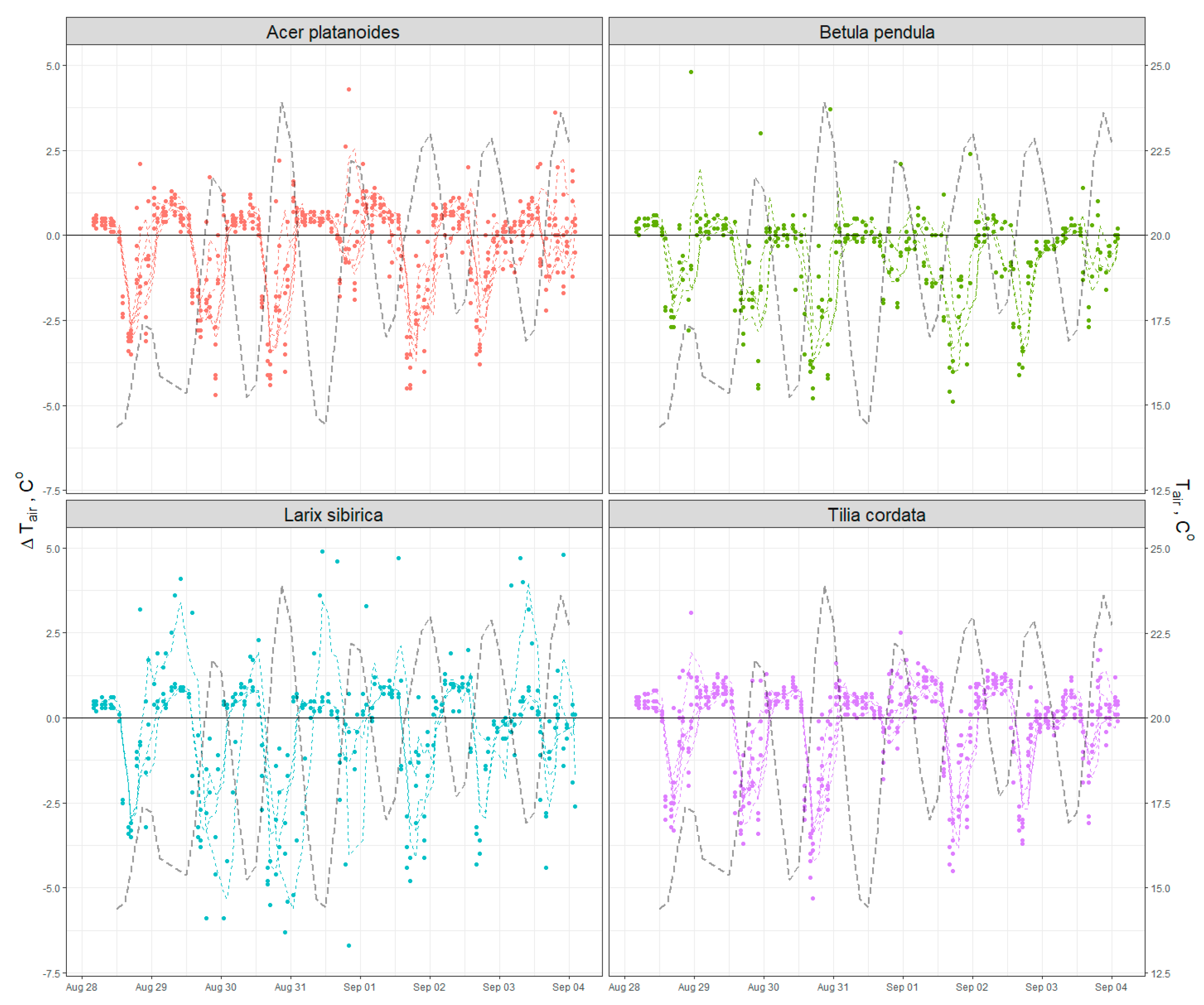
2.2.2. Climate Regulation via Air Temperature Control

We used direct measurements of temperature changes based on the difference between data from thermo-hygrometers of individual TT, measuring climate parameters at 3 m height under the crown space, and TT-R (reference outside station). Temperature measurements were taken by the TT device with a measuring cycle of 1.5 h as for all the other parameters.

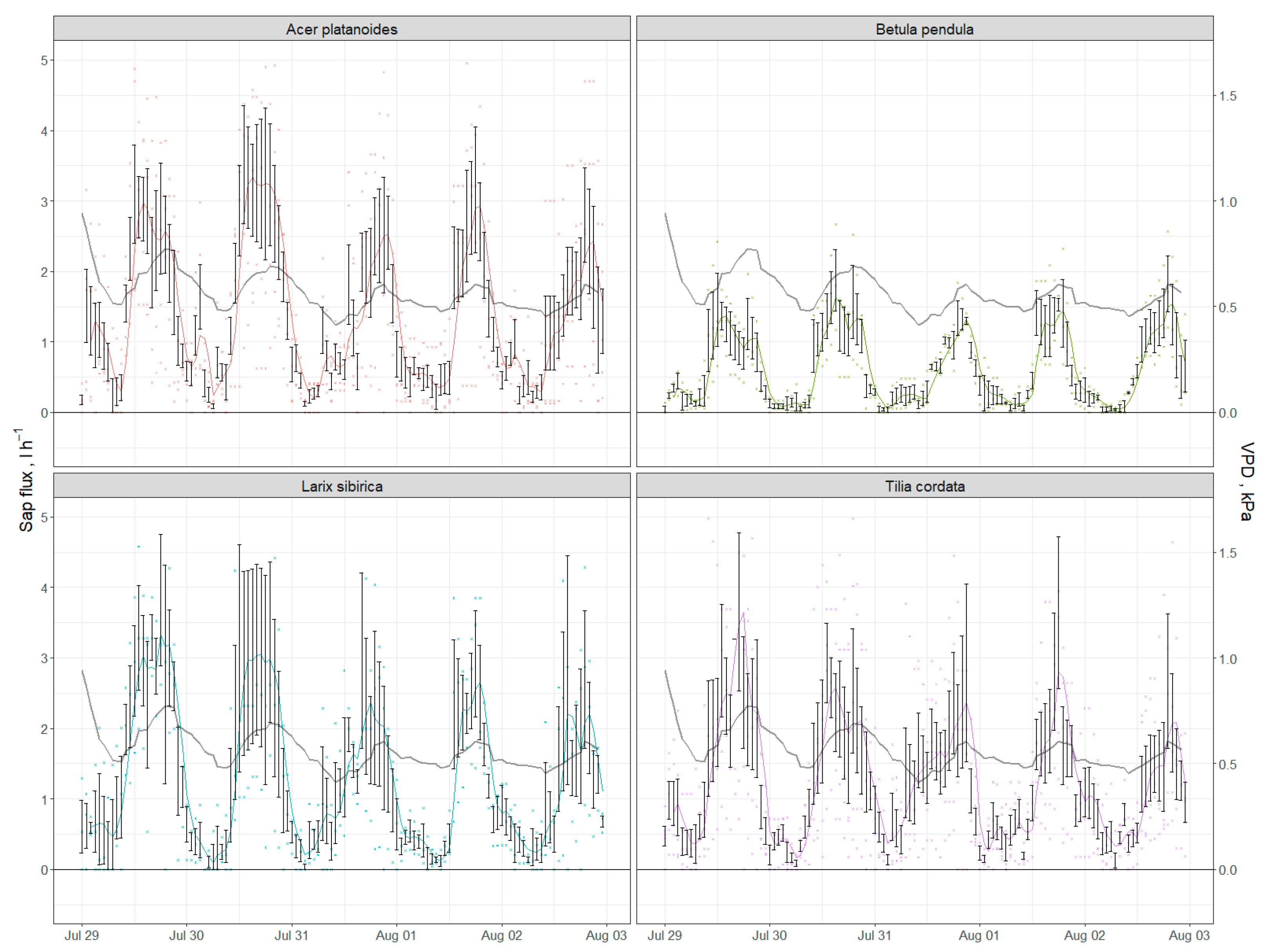
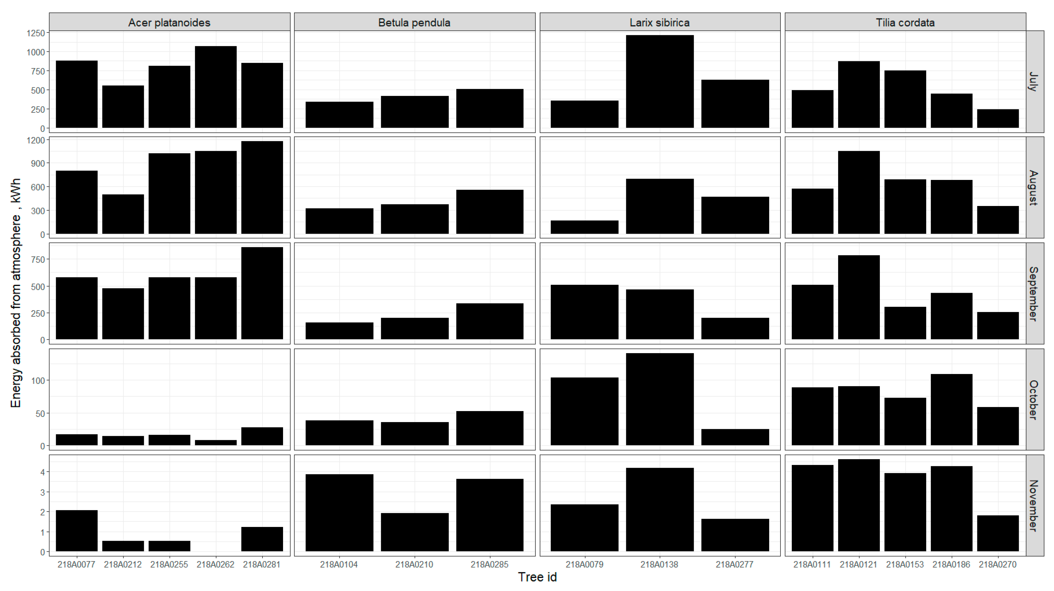
2.2.3. Water Fluxes and Energy Consumption through Transpiration

The transpiration rate of whole plants is closely approximated by the sap-flow rate in the main stem or trunk. We implemented the thermal dissipation method in the TT+ platform, first developed by Granier [74]. Granier’s original method is based on the assessment of the amount of heat dissipated from a heated probe in relation to a reference probe in proximity (about 10 cm in our case), with continuous heating. To reduce energy consumption, the method was modified according to Do et al. [43,75] and instead of continuous heating, cycles of cooling (80 min) and heating (10 min) were used. The heated and reference probes of TT+ were installed into the tree trunk at a vertical distance of 10 cm. The probes had a diameter of 2.5 mm each and were installed at the depth of 2.5 cm. The TT+ heat dissipation probe was installed at the 3.5 m height of the trunk and was well protected from direct sun heating by the canopy and the northernly orientation. The sap wood area for each tree was assessed by using literature data on its relation to tree diameter [76,77,78]. Sap flow was calculated with the assumption that the whole trunk sapwood area was conducting water. It was assumed that daily transpiration was equal to daily sum of sap flow.
The energy absorbed by the tree for transpiration was calculated based on the equation:
L = λT,
where λ is the energy spent in transpiration (the latent heat for vaporization of water = 2264.705 KJ/Kg) and T is the transpiration, which is calculated by sap-flow density and the estimated sapwood area.
We have considered that the potential runoff mitigation of urban trees as ecosystem service indicators can be shown as the ratio of transpiration (T) to precipitation (P):
Rp = T/P
where both terms are calculated using mm. Tree-level transpiration has been recalculated per unit of crown area. The equation could be, in principle, implemented with evapotranspiration, with evaporation estimated by simple meteorological models and canopy interception through LAI, but in the present paper we simplify the approach to derive a runoff mitigation indicator, represented by Rp.

2.2.4. LAI

There are many methods and protocols to estimate LAI [79,80]. Light transmission through the canopy as porous media can be treated according to Beer’s Law [81]. In this way LAI can be estimated by the extinction of photosynthetic light radiation through the canopy [82]. Photosynthetically-active radiation was measured outside and below the canopy (with TT-R and TT+ spectrometers, respectively). Since the light is also blocked by the woody components of canopy (i.e., branches and twigs), the extinction of the light profile gives the PAI (plant area index) as follows:
PAI = LAI + WAI = ln ( PAR TT + PAR TTR ) k
PAI consists of wood area index (WAI) and leaf area index (LAI). Assuming that WAI is constant throughout the vegetation period and LAI = 0 after defoliation (second part of October and November), WAI for each tree was calculated as the mean PAI of November. Light extinction coefficient k was calculated per each species utilizing LAI light measurements at the foliage peak with a hemispherical photo done with Kodak PIXPRO SP360 and Hemisfer software [83].

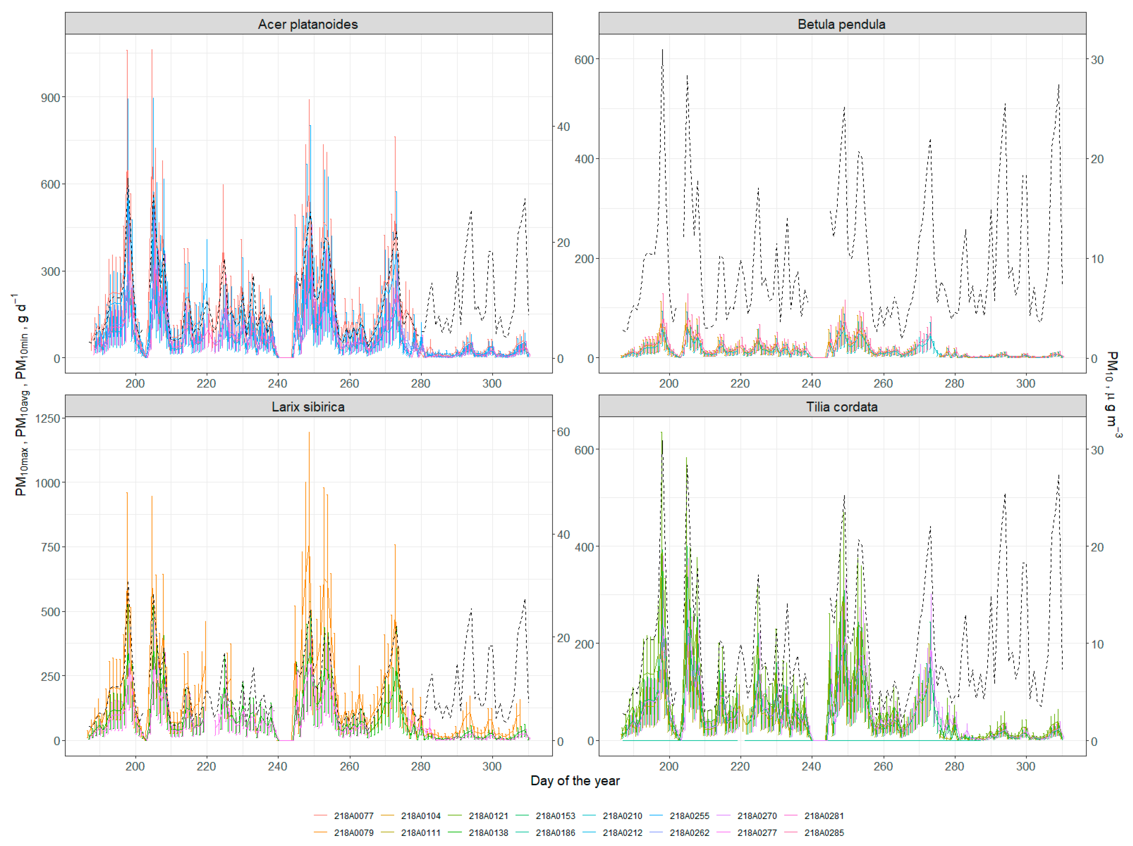
2.2.5. Particulate Adsorption

Dry deposition of solid particles on the canopy was calculated according to i-Tree Eco dry deposition model [46]:
P ads = V d C   V d =   V dPM 10 avgB · W A I + L A I W A I + L A I P M 10     V d , min =   V dPM 10 min · W A I + L A I W A I + L A I P M 10     V d ,   max =   V dPM 10 max · W A I + L A I W A I + L A I P M 10  
where C is the PM10 concentration (g m−3), Vd the velocity of deposition (m s−1), LAIPM10 the leaf area index for pollutant deposition (m2 m−2), and VdPM10max, VdPM10avg, and VdPM10min are maximum, average, and minimum deposition velocity for PM10—0.0064 ms−1, 0.0025 ms−1, and 0.01 ms−1, respectively. Values were multiplied by canopy area to show adsorption per individual tree. Pollutant concentration was obtained from nearby open access PM10 sensors via the sensor.community web portal in Moscow (https://sensor.community).

2.3. Data Processing

Data collection with TreeTalker+ devices was organized according to the following scheme. All types of devices (TT+ and TT-R) made measurement every 90 min, stored data in internal memory, and then according to a predefined time window transmitted data to the gateway (TT-cloud) device via low-power wide-area network (LoRa) wireless networking protocol. The TT-cloud device is a gateway, whose purpose is to collect data from all TT devices on site, store it and then transmit it to an online database via WiFi or wireless mobile networks.
All remote data were collected and processed using the R computing language [84]. Field data was organized in a table and added to computation during early stages of processing. All measurement which deviated by more than three standard deviations from the weekly mean was filtered out. Filtered data was linearly interpolated. Most of data gaps were less than four measurements (6 h) and the maximum gap was 44 measurements (66 h) due to water-damaged electronics after heavy rain. Data were filled with data from trees with the closest parameters (species, trunk diameter, height, canopy size, and position on site). Statistical analysis of results (correlation analysis) was also performed in R environment.

3. Results and Discussion

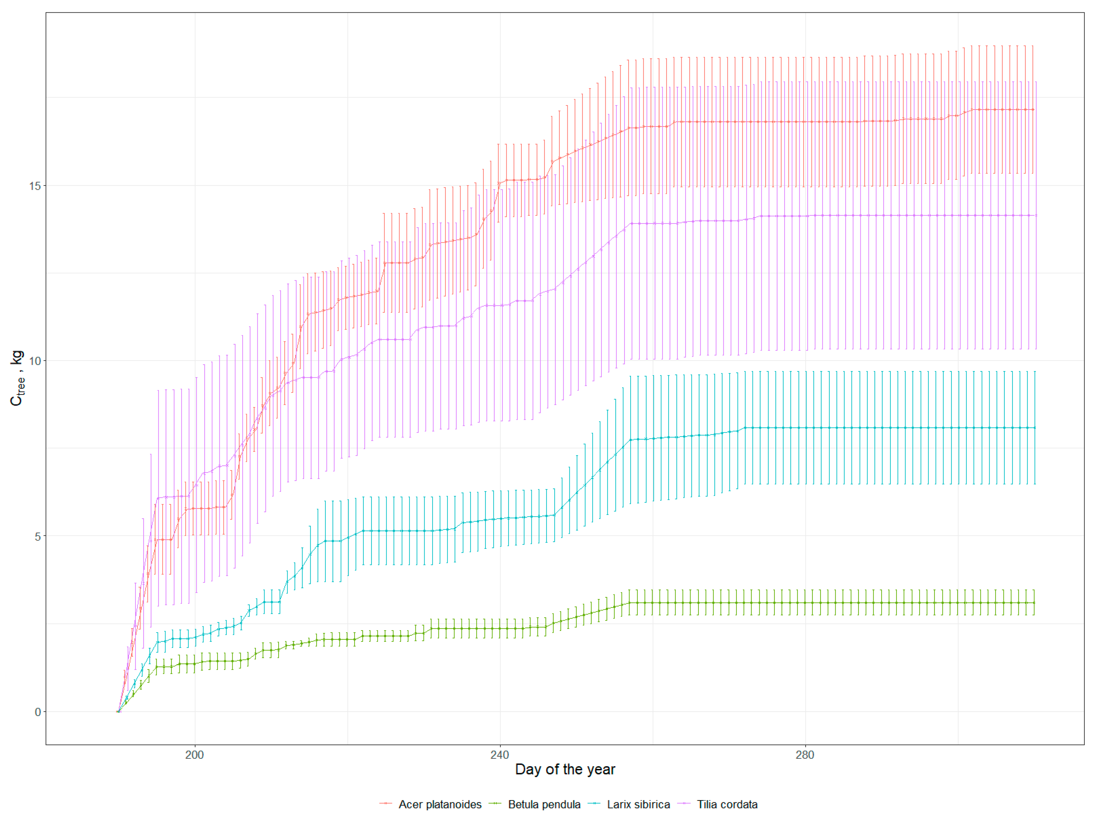
3.1. Carbon Sequestration
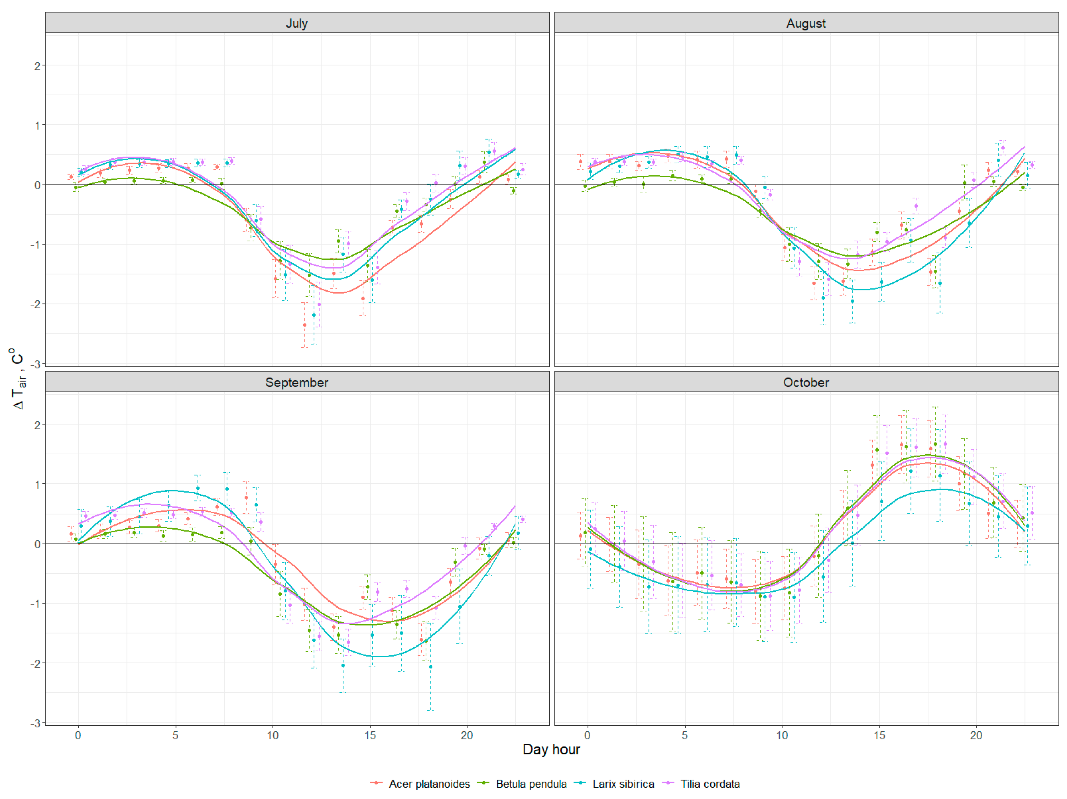
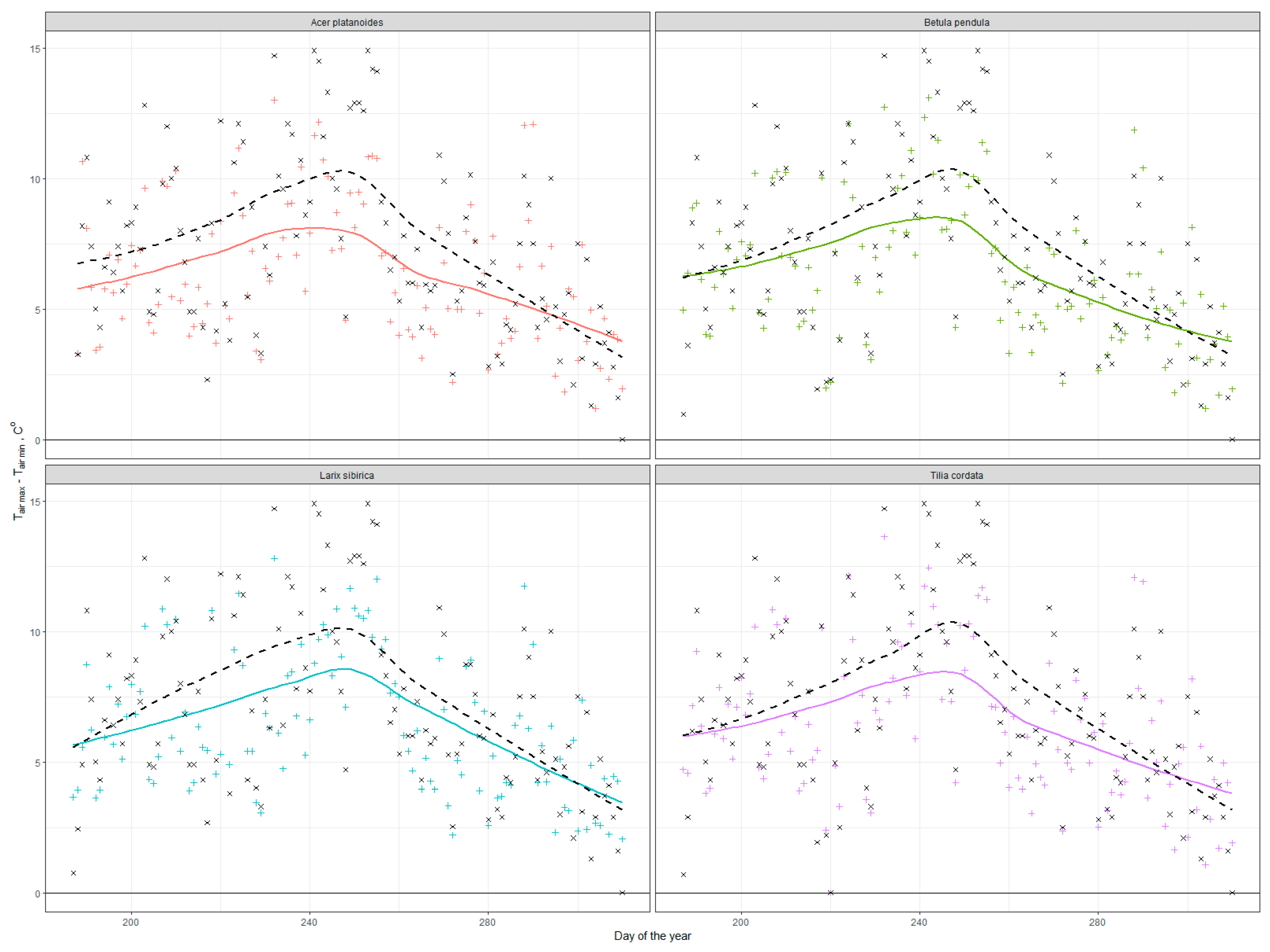
As the diameter increment is an important component of carbon storage across the season, relative biomass accumulation was calculated using Equation (1). The growth dynamics show biomass increase until the end of September (around day 260 of the year) due to the warm autumn (Figure 3).
Betula pendula growth rates ranged from 2.19 to 2.79 kg C per tree along the season and they represent the lowest values among the investigated trees. Acer platanoides growth rates ranged from 8.35 to 15.3 kg C per tree along the season. Tilia cordata growth rates were slightly lower than those for Acer platanoides, ranging from 1.76 to 6.27 kg C, showing a marked individual variation. Larix sibirica trees showed similar growth rates with values ranging from 4.95 to 7.66 kg C per tree. In total the average amount of carbon accumulated in the tree biomass for the investigated species was 11.58 ± 1.47 kg C (Acer platanoides, ± standard error), 2.5 ± 0.15 kg C (Betula pendula), 6.03 ± 1.31 kg C (Larix sibirica), and 10.89 ± 2.89 kg C (Tilia cordata). The overall uncertainty in the biomass carbon sequestration estimates arising from the propagation of measurements and parameter uncertainties, was on average 3.6% ranging from a minimum of 2.3% (Larix spp.) to a maximum of 5.6% (Betula spp.). In general carbon sequestration related to resultant biomass increment significantly was correlated mostly to tree stem diameter, exhibiting a Pearson r coefficient of 0.87, followed by canopy size and tree transpiration with mutually similar, yet much weaker, relations (r = 0.39 and 0.36, respectively).
General knowledge of urban tree-carbon dynamics, including the balance of growth, mortality, and planting rates is quite data-limited [47]. Although the carbon stock density of urban green areas is generally smaller than that of forests, the potential storage capacity is still considerably higher [85,86]. Growth rates of urban trees may be accelerated by the heat island effect, as a result of increased temperature, longer growing season, and potentially higher N deposition [87]. Conversion of diameter growth in biomass and hence carbon sequestration is very much related to the BEF coefficients which we derived by [70], specifically for the Russian environment. One of the most comprehensive studies on urban tree-carbon sequestration is one across a wide range of US cities [47]. These authors showed an average annual net carbon uptake, per tree, of about 0.226 kg C m−2 year−1. Unfortunately, they did not analyze individual species performance but only the overall carbon accumulated by the unit of green area. Scaling larch trees carbon sequestration per unit of crown area we obtain an average value of 0.14 ± 0.04 kg C m−2, which is the closest result in relation to Nowak et al. [47], but for broad leaved species this parameter was more than two times higher (with a maximum of 0.48 ± 0.14 kg C m−2 over the study period for Acer platanoides). For Tilia cordata of the same age, Moser et al. [88] reported a mean annual carbon uptake of 4.58 kg C per tree (2.48–7.12) which is lower compared with our estimate of 10.89 ± 2.89 kg C (4.3–17.79).
However it compares well with our mean annual growth increment of 4.5 ± 1.18, which was determined using the same approach using total stock and tree age. Using a continuous dendrometer with larch species of about the same age (60 years), Deslauriers et al. [89,90] found an annual radial increment of 1.8 mm which is comparable with our estimates of 2.07 ± 0.33 mm. Using a large national inventory for birch trees in Finland, Repola et al. [91], found an annual radial increment of 1.1 mm, while we observed an growth of 2.79 ± 0.91 mm. However, we have to consider the difference between forests and isolated urban trees. This also showed the importance of considering the difference between the current and the mean increment in future carbon sequestration analyses. Although it is difficult to compare our data with existing annual growth rates, due to the lack of full season data coverage (about four out of six months) our data show a reasonable consistency with the annual mean increment of the same trees. More importantly they confirm the possibility of monitoring the carbon sequestration of urban trees in real-time.

3.2. Cooling Effect

The local climate control from an ecosystem-services perspective is the mitigation of extreme temperatures and providing a more comfortable urban microclimate. In Figure 4 the diurnal difference mean changes of temperature between the reference station and the space under the tree crown is presented as the mean monthly day, for the investigated species. During the day, the temperature difference was maximal, peaking early afternoon in July, August, and September. This dynamic was reversed in October. During the day trees were cooling the surrounding air via shading and evaporative cooling, showing an effect of up to about 2 °C degrees with the external temperatures (Appendix B). In October, all the species showed a warming effect at midday, of the same order. An opposite behavior is recorded for nighttime periods where, usually during summer months, trees were slightly warmer than the surrounding air. In October they showed a cooling effect during the night.
Another important effect of trees is the mitigation of climate extremes. For this purpose, we have estimated the daily differences between maximum and minimum temperatures of the reference station and the individual tree recording (Figure 5). While temperature amplitudes outside of the canopy (the black line) reached a maximum of about 10 °C degrees in August, under the canopy this amplitude was 3 °C degrees lower. All the species showed similar dynamics through the investigated period, but under the larch, temperature extremes were more like the reference station both during summer and particularly after autumn leaf drop.
These findings correspond well to [60], who explained observed seasonal dynamics of temperature reduction rates by differences in transpiration and to [92], who also found that within the canopy radius of 4.5 m of Acer platanoides or Tilia cordata trees, daytime air temperature decreased up to 3.5 °C during August in comparison to the unshaded surrounding area. Our results agree with a meta-analysis study, which showed relations between individual tree characteristics and daily/seasonal temperature reduction dynamics in different climate and urban conditions [92]. Air temperature reduction by urban green infrastructure of about 0.5–2.5 °C degrees was also shown in several papers, which used computational modeling [52,93] and satellite based data for land-surface temperature [94,95].

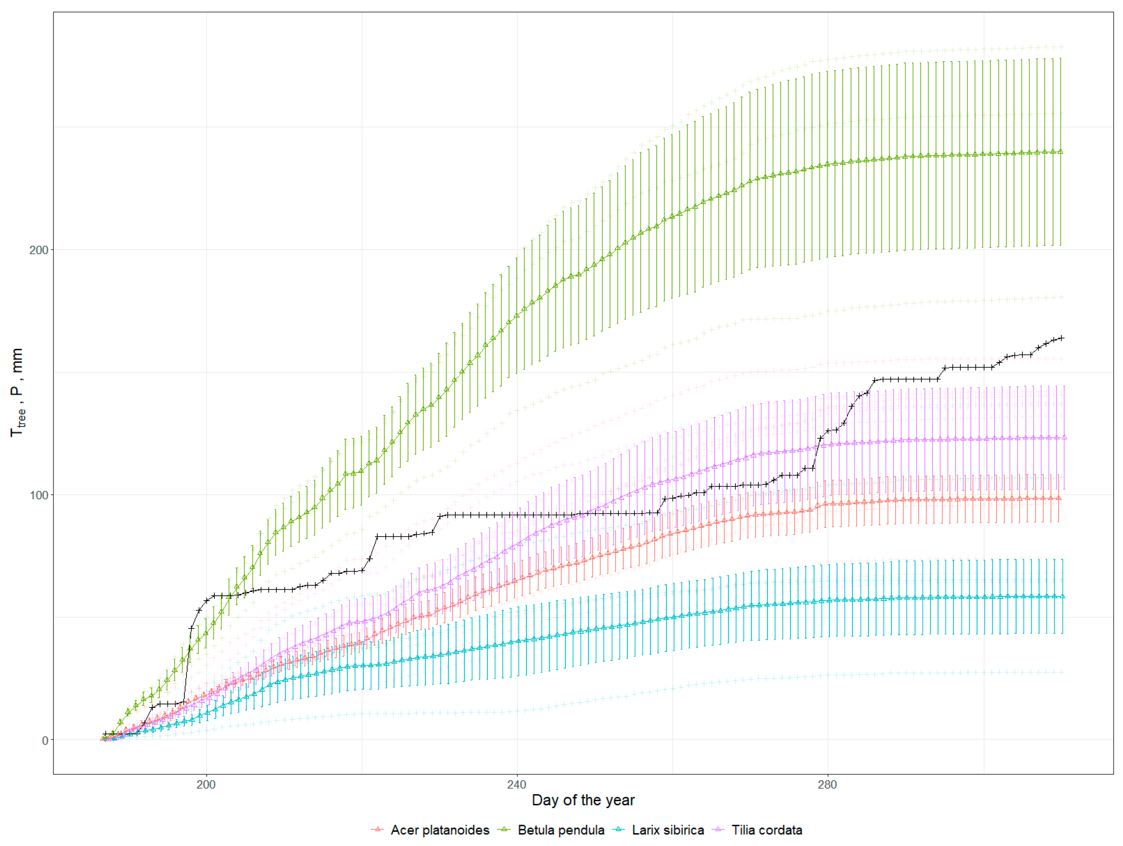
3.3. Run-Off Mitigation and Energy Consumption by Trees via Transpiration

Ensembles of transpiration daily patterns show the typical diurnal behavior modulated by changing environmental parameters, with a variation in the onset and the peak of the transpiration cycle across the individuals, particularly in Acer platanoides and Tilia cordata, showing the variation of conditions to sun exposure (Appendix C). Sap flux during night for all individuals was negligible, while during the day it increased up to 3 lh−1 for Betula pendula trees and 5 lh−1 for several Tilia cordata and Acer platanoides trees in July. Maximal values of daily flux were detected for all species in July, and reached 8 lh−1 for Larix sibirica, 7.6 lh−1 for Acer platanoides, 5.9 lh−1 for Tilia cordata, and 3.8 lh−1 for Betula pendula, while average daily (24 h) flux for those species in July was 2.90 ± 0.08, 2.85 ± 0.08, 2.18 ± 0.05, and 1.74 ± 0.04 lh−1, respectively. In following months, sap flux values gradually decreased for all species.
For the purpose of the current study we report the amount of cumulated transpired water in relation to seasonal rainfall. The units are expressed in mm of water, where for each of the trees, transpiration rates have been converted to mm by using the tree canopy area. The main purpose is to show, from an ecosystem-services perspective, the role of trees to complement (or support) the drainage systems by actively lowering the soil water content, thus increasing its marginal water storage capacity and mitigating the volume of stormwater entering the drainage channels. Our results show that Acer platanoides and Tilia cordata trees consumed 107 ± 39 mm (± standard error) and 122 ± 32 mm of water, respectively, through the investigated period. Larix sibirica trees reduced 66 ± 40 mm of water, while young Betula pendula trees reduced 240 ± 53 mm (Appendix A, Figure 6). In general, this cumulative process was mostly linear with some differences in rates that were found to be associated with different VTA scores. On the other hand, there was no significant response to the heavy rains. According to our data we can say that up to 130 ± 28% (± standard error) of precipitation can be transpired per square meter of canopy area for Betula pendula. Meanwhile mature broadleaf trees such as Tilia cordata and Acer platanoides transpired 66 ± 17% and 58 ± 21% of precipitated water during the study period. The only investigated coniferous species showed minimal values yielding 36 ± 21% of precipitated water transpired. The high values of Betula pendula, although showing a lower rate of transpiration per tree, can be explained by a greater efficiency per canopy area. This also shows how the birch trees can very efficiently utilize soil moisture storage.
For the investigated period, the ability of individual trees to transpire precipitated water volume around them positively correlated with the size of those species canopies. This supports the findings of similar works [88,96]. Taking into account all the trees within the study location, the total annual plot rainfall (excluding any extreme rainfall events) was approximately equal to total transpiration, what was shown for boreal urban trees of other municipalities [61,63]. Such information obtained in real-time could considerably contribute to cities’ stormwater management [97,98,99]. On the other hand, it is widely discussed that rain interception by leaf buffering during heavy rains also contributes to run-off mitigation [66,100,101], which is based on leaf area index, as discussed further in the text.
Using the energy balance equation (Equation (3)) it was possible to estimate the amount of absorbed radiation that is subtracted from the environment due to transpiration. The diurnal graph shows the increase of the transfer latent heat (L) during the daytime when transpiration starts following the sunrise (Figure 7). The daily range of adsorbed energy during July and August was 0.5–2.2 kWh for Acer platanoides, Larix sibirica, and Tilia cordata trees, while for Betula pendula it was a bit lower (0.2–1.5 kWh). Already in September there was a decrease in absolute numbers below 1.2 kWh for all species, but the range for Acer platanoides was 0.6–1.2 kWh, and for Betula pendula again, on a level of 0.1–0.6 kWh. In comparison, during October and November the lowest values were shown by Acer platanoides trees (with a range 0.1–0.2) while for all other species it was 0.2–0.8 kWh. On average, during the investigated period 2471.2 ± 266 kWh (±standard error) of energy was accumulated by Acer platanoides, 1379.4 ± 436.7 kWh by birch, 2140 ± 676.8 kWh by larch, and 2221.7 ± 385.4 kWh by Tilia cordata trees. The differences between individuals are noticeable (Appendix D).
Energy latent heat fluxes varied between tree species, individual trees, and seasons. We found that main variability between individual trees was due to the difference in stem size and canopy area. While there are few publications investigating the energy balance of boreal urban trees, we showed comparable measurements for Tilia cordata in summer months to another study [88].

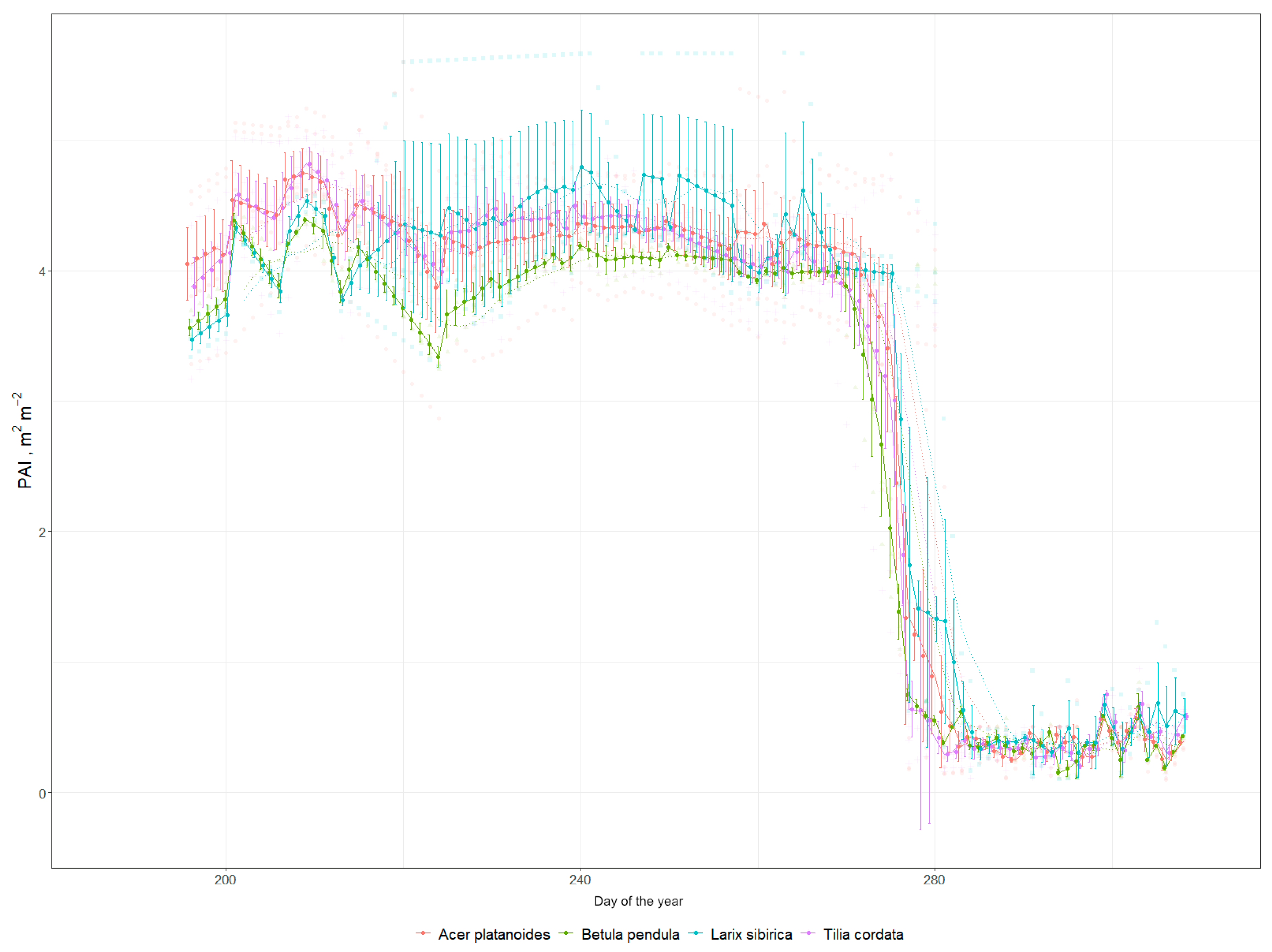
3.4. LAI as a Proxy for ES Provision

The dynamics of LAI are a good proxy for several types of ES, such as wind velocity reduction, noise reduction, pollution regulation, and erosion protection via leaves acting as a buffer (see references from Table 2). From our radiation sensor we can calculate the overall PAI, that is, a sum of the leaves and wood (bark) light interception effects. Thus, after comparing periods with and without leaves we could derive both leaf and wood area index. These periods are clearly visible in Figure 8 where we can easily distinguish the time of defoliation which lasted for one week in the first days of October. Average LAI for all trees (Appendix A) was 3.77 with less variation in Betula pendula (3.5–3.7) and Larix sibirica (3.6–3.9) and higher variation for Acer platanoides (3.2–4.3) and Tilia cordata (3.4–4.3).
Despite the clear pattern shown in Figure 8, LAI, estimated by the spectrometer, was influenced by the angle of view of the spectrometer, which is ±20° and positioned in the north side of the trunk, thus recording only one section of the crown. For a better absolute determination it is necessary to compare the sensor with more precise techniques (e.g., camera with fish-eye lens or other LAI meters) which are essential for calibration and validation [80,102]. That said, the absolute values (3–4) are comparable to most of the papers [80,82,103] in similar species. While the strong correlation between LAI and DBH and also between LAI and tree height was shown previously for Canadian and Bavarian boreal forests [103,104] our results did not allow us to confirm this correlation. This lack of correlation is possibly explained by the small number of trees in consideration and the urban conditions of our study site [105]. However the real-time dynamics of LAI and WAI is the advantage of our device which is important for plant physiological processes and models [106].

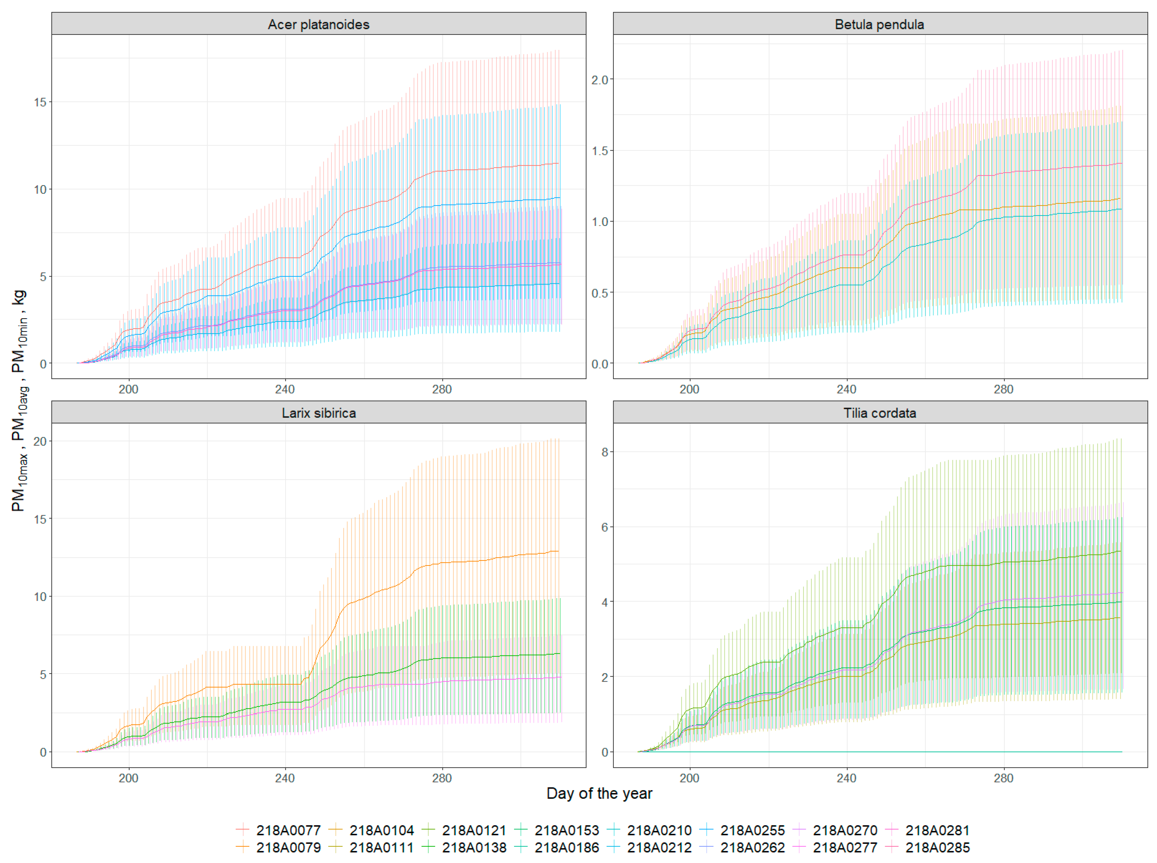
3.5. Particulate Adsorption

Particulate adsorption is influenced by two main parameters — PAI and particulate concentration in air, according to the model described in Methods. The adsorption dynamic during the investigated period mostly reflected the changes in particulate matter concentration, which showed peaks at the end of July and beginning of August, and again in September and late November. While the reasons for these pollution dynamics were not our focus, we can say that the average absorption rates differed among the investigated trees, mostly due to their LAI. The lowest adsorption rates were shown by Betula pendula trees with an average of 9.3 g per day, and the highest were Acer platanoides and Larix sibirica trees with 51.2 and 51.4 g per day, respectively. Tilia cordata trees were in the middle with 25.5 g per day per tree (Appendix E). The highest adsorption peaks (in terms of maximum deposition velocity) were up to 1200 g (Larix sibirica) during several days with high concentrations in the air. This parameter showed drastic variation across time. The cumulative particulate mass adsorption over the season was 7.7 ± 1.5 kg for Acer platanoides (± standard error), 7.7 ± 2.1 kg for Larix sibirica, 3.8 ± 0.2 kg for Tilia cordata, and 1.4 ± 0.1 kg for Betula pendula (Figure 9, Appendix A).
Sæbø et al. [68] showed that Betula pendula improves air quality by particulate adsorption much better than Acer platanoides and Tilia cordata, however tree size should be taken into account as a factor to interpret the results of our study. It is well known that healthy large trees remove about 60 times more pollution annually than healthy small trees [67]. Additionally, leaf wax or leaf hair density and topography also have great influence [68,107]. In our case we could not include leaf morphology or topography since our estimation was based on LAI. However the total adsorption by tree seems comparable with several works yielding an average of 0.5–5 g m−2 rates of adsorption in different cities [18,108,109], which resulted in 10–200 g of particulate matter adsorption daily per tree. Thus, our results from the high-traffic Moscow center look comparable.

4. Conclusions

According to our findings we can summarize ecosystem-services estimation for an individual tree as averaging 8.61 ± 1.25 kg (± standard error) of carbon stored, 137 ± 49 mm of water transpired, 2167 ± 181 kWh spent for microclimate regulation, and 5309 ± 808 g of PM10 adsorbed per the investigated period (July–November 2019). These numbers could be easily transformed to monetary values with the use of local prices for each of these services [110]. For Moscow, it would amount to about $150 per tree during the study period, mostly due to energy and particulate adsorption.
There are several approaches to provide ES information for the green infrastructure in urban areas. However, most of the inventory approaches, even when based on high resolution imaging, are limited by the temporal resolution which sometimes is important for detecting an early onset of ES decline. Our results show that an IoT tree-level network, using individual tree physiology sensing devices, such as TreeTalker+, or other similar devices, can be used in principle for monitoring urban green infrastructure ES in real-time. Furthermore, for some of the ES indicators, (e.g., water and cooling effects), they are most often based on models with indirectly-derived parameters [111]. Having real-time and individual tree data can improve our predictions and urban green infrastructure planning. There are several advantages for increasing the granularity of ES monitoring, particularly in that individual trees can be managed with a greater accuracy. The cost of monitoring is therefore critical for IoT expansion in green infrastructure monitoring. In recent years technological development and low cost microprocessors, traditionally used in automation and industry processes (Industry 4.0), are creating new opportunities for their expansion in environmental monitoring, which we could define as a Nature 4.0 transformation [36]. Typically, the total cost of a cluster of 20 trees is about 6000 euros, including the gateway, which corresponds to about 300 euros per tree. A single gateway can host up to 48 trees and the cost could decline with increasing monitored trees.
However, there are limitations and improvements to be considered in future work. First of all, the power consumption of the TreeTalker+ devices, used in the current work, is still a big limitation. Batteries need to be replaced every 1–1.5 months which requires a considerable human resource input. New batteries are being developed with much larger capacity that in principle could extend the battery life duration. In terms of improvement, a new IR sensor for distance sensing of canopy temperature could be very useful for improving the energy balance estimation and cooling effects. In particular, the installation of an anemometer will provide additional data on wind speed in the canopy, which influences the delivery of several ES. In addition, simple PM 2.5–10 optical devices can be included in the processor platform to get useful data on air quality using trees as monitoring stations. Further studies need to be conducted, but a noise sensor and microphone could also be included with the aim to provide useful information on the noise pollution and “soundscape” quality generated by trees in parks [35,112] and also to evaluate associated biodiversity with the help of recorded bird songs [34,113]. Nevertheless, the technical development of sensors along with people engagement to citizen science will be inevitable [32,114,115], thus it will be important to adapt them to the task of monitoring those parameters that are important for urban planning decisions [116].
Among the indicators presented in the article, perhaps not all of them can be directly used for practical purposes. For example, wind speed as well as air temperature and humidity under the canopy of city trees can be presented “as is” for the general public. However, in order to provide clear information on the quality of the urban environment associated with green infrastructure for public consumption, specific scales of air quality, microclimate comfort, and noise pollution levels should be developed. On the other hand, for spatial planning tasks, it will be useful to create an urban tree database on annual or seasonal indicators of ecosystem services provided by tree species at their specific age, height, and condition. This could be very useful for operational management of urban green infrastructures. [117]. In addition, it is also necessary to take into account disservices associated with urban trees such weakened and diseased trees falling on cars, infrastructure and buildings, and the allergic reaction of people to tree pollen [118,119]. These parameters should also be continuously monitored and reported in real-time for rapid response or timely prevention.

Author Contributions

Conceptualization and methodology, R.V. and V.M.; software, A.Y. and L.B.M.; validation, G.S. and L.B.M.; investigation, G.S., L.B.M., O.F., I.S., and A.Y.; data curation, A.Y.; writing—original draft preparation, V.M.; writing—review and editing, V.M., R.V., L.B.M., and S.C.; visualization and formal analysis A.Y.; supervision, R.V.; project administration and funding acquisition V.V. All authors have read and agreed to the published version of the manuscript.

Funding

Monitoring and modeling ecosystem services of urban trees was supported by Russian Scientific Foundation Project # 19-77-300-12. Data processing and analysis was supported by “RUDN University program 5–100”.

Acknowledgments

We thank two anonymous reviewers for their valuable comments and candidate Christopher Ryan for proof-reading, which helped to improve the manuscript.

Conflicts of Interest

The authors declare no conflict of interest.

Appendix A

Table A1. Tree description and summary of ecosystem services produced by each tree per investigated period (July–November 2019).
Trees DescriptionBiomass CarbonTranspiration and PrecipitationEnergy Absorbed - L, kWhPM10 Particles Absorbed, kgLeaf and Wood Indexes
idAge GroupTree Height, mStem Diameter, cmStem Radial IncrementCanopy Area, m2VTABEFBCEFR/STotal Tree-carbon Stock, kgAverage Annual Carbon IncrementCurrent Annual Increment kgCarbon Stored per Canopy Area, kg m−2Transpiration, mmPrecipitation, mmRatio of Precipitation Evaporated, mmPM10maxPM10avgPM10minPAI, m2m−2WAI, m2m−2LAI, m2m−2
Acer platanoides
218A007750–602035.73.455.721.31.10.3580.010.613.00.268.0183.50.4245418.011.54.54.80.54.3
218A021250–601533.73.227.631.31.10.3393.67.28.80.396.2183.50.516157.34.61.84.00.53.5
218A025550–602034.43.255.321.31.10.3559.810.212.50.274.0183.50.4250615.19.63.84.30.43.8
218A026250–601334.73.328.511.31.10.3373.76.88.40.3155.2183.50.827397.95.02.04.80.64.2
218A028150–601445.84.335.841.31.10.3685.012.515.30.4140.4183.50.8304211.97.63.03.60.43.2
Mean 16.836.93.540.6 518.49.411.60.3106.8183.50.62471.212.07.73.04.30.53.8
SE 1.72.50.27.0 66.01.21.50.039.30.00.2266.02.31.50.60.20.00.2
Betula Pendula
218A010450–601121.72.77.611.20.80.280.41.52.40.3180.5183.51.011572.01.30.54.00.43.5
218A021030–401121.02.66.411.20.80.273.71.32.20.3255.5183.51.412262.01.30.54.00.43.6
218A028530–401123.93.08.211.20.80.293.91.72.80.3282.7183.51.517562.51.60.64.10.43.7
Mean 11.022.22.87.4 82.71.52.50.3239.6183.51.31379.42.21.40.54.00.43.6
SE 0.07.00.90.6 8.30.20.40.152.90.00.3436.70.10.10.00.10.00.1
Larix Sibirica
218A007980–1002532.22.065.931.10.80.3421.17.76.30.127.5183.50.1170117.511.24.44.70.83.9
218A013880–1001940.72.637.421.10.80.3519.59.57.80.2106.9183.50.632389.86.32.54.10.53.6
218A027780–1002426.11.632.321.10.80.3272.55.04.10.165.3183.50.414818.85.62.24.00.43.6
Mean 22.733.02.145.2 404.47.46.00.166.6183.50.42140.012.17.73.04.30.53.7
SE 2.25.20.312.8 87.91.61.30.039.70.00.2676.93.42.20.80.20.10.1
Tilia Cordata
218A011150–601228.05.320.031.20.70.3137.62.56.10.3132.1183.50.721956.54.11.64.30.53.8
218A012150–601737.97.131.311.20.70.3345.06.315.30.5142.1183.50.833706.74.31.74.60.64.0
218A015340–501435.36.721.121.20.70.3245.64.510.90.5137.3183.50.721965.43.51.44.40.44.0
218A018640–501740.47.619.531.20.70.3400.17.317.80.9136.5183.50.721524.93.11.23.80.43.4
218A027030–401125.24.722.431.20.70.396.81.84.30.264.4183.50.411966.54.11.64.40.54.0
Mean 14.133.46.322.9 245.04.510.90.5122.5183.50.72221.76.03.81.54.30.53.8
SE 1.33.30.62.4 65.01.22.90.132.70.00.2385.40.40.30.10.10.00.1

Appendix B

Figure A1. Daily dynamics example of the air temperature (Tair—dashed line) and the difference (dT—colored line) under and outside of the canopy (TTair–TTRair).
Forests 11 00775 g0a1

Appendix C

Figure A2. Example of flux dynamics per species for several days.
Forests 11 00775 g0a2

Appendix D

Figure A3. Energy removed from atmosphere monthly by each investigated tree.
Forests 11 00775 g0a3

Appendix E

Figure A4. Dynamics of atmospheric particulate matter with diameter less than 10 micrometers (PM10)—averaged daily concentration in air (dashed line) and amount of PM10 absorbed by investigated trees daily (line shows average value, while whiskers denote minimum and maximum).
Forests 11 00775 g0a4

References

  1. Dye, C. Health and Urban Living. Science 2008, 319, 766. [Google Scholar] [CrossRef] [PubMed]
  2. Bettencourt, L.M.A.; Lobo, J.; Helbing, D.; Kuhnert, C.; West, G.B. Growth, innovation, scaling, and the pace of life in cities. Proc. Natl. Acad. Sci. USA 2007, 104, 7301–7306. [Google Scholar] [CrossRef] [PubMed] [Green Version]
  3. Frumkin, H. Healthy Places: Exploring the Evidence. Am. J. Public Health 2003, 93, 1451–1456. [Google Scholar] [CrossRef] [PubMed]
  4. Lederbogen, F.; Kirsch, P.; Haddad, L.; Streit, F.; Tost, H.; Schuch, P.; Wüst, S.; Pruessner, J.C.; Rietschel, M.; Deuschle, M.; et al. City living and urban upbringing affect neural social stress processing in humans. Nature 2011, 474, 498–501. [Google Scholar] [CrossRef] [PubMed]
  5. Grimm, N.B.; Faeth, S.H.; Golubiewski, N.E.; Redman, C.L.; Wu, J.; Bai, X.; Briggs, J.M. Global Change and the Ecology of Cities. Science 2008, 319, 756. [Google Scholar] [CrossRef] [PubMed] [Green Version]
  6. Seto, K.C.; Guneralp, B.; Hutyra, L.R. Global forecasts of urban expansion to 2030 and direct impacts on biodiversity and carbon pools. Proc. Natl. Acad. Sci. USA 2012, 109, 16083–16088. [Google Scholar] [CrossRef] [PubMed] [Green Version]
  7. Bolund, P.; Hunhammar, S. Ecosystem services in urban areas. Ecol. Econ. 1999, 29, 293–301. [Google Scholar] [CrossRef]
  8. Guo, Z.; Zhang, L.; Li, Y. Increased Dependence of Humans on Ecosystem Services and Biodiversity. PLoS ONE 2010, 5, e13113. [Google Scholar] [CrossRef]
  9. Krausmann, F.; Lauk, C.; Haas, W.; Wiedenhofer, D. From resource extraction to outflows of wastes and emissions: The socioeconomic metabolism of the global economy, 1900–2015. Glob. Environ. Change 2018, 52, 131–140. [Google Scholar] [CrossRef]
  10. Blanusa, T.; Garratt, M.; Cathcart-James, M.; Hunt, L.; Cameron, R.W.F. Urban hedges: A review of plant species and cultivars for ecosystem service delivery in north-west Europe. Urban For. Urban Green. 2019, 44, 126391. [Google Scholar] [CrossRef]
  11. Gómez-Baggethun, E.; Barton, D.N. Classifying and valuing ecosystem services for urban planning. Ecol. Econ. 2013, 86, 235–245. [Google Scholar] [CrossRef]
  12. Lovell, S.T.; Taylor, J.R. Supplying urban ecosystem services through multifunctional green infrastructure in the United States. Landsc. Ecol. 2013, 28, 1447–1463. [Google Scholar] [CrossRef]
  13. Neugarten, R.A.; Langhammer, P.F.; Osipova, E.; Bagstad, K.J.; Bhagabati, N.; Butchart, S.H.M.; Dudley, N.; Elliott, V.; Gerber, L.R.; Gutierrez Arrellano, C.; et al. Tools for Measuring, Modelling, and Valuing Ecosystem Services: Guidance for Key Biodiversity Areas, Natural World Heritage Sites, and Protected Areas, 1st ed.; Groves, C., Ed.; IUCN, International Union for Conservation of Nature: Gland, Switzerland, 2018; ISBN 978-2-8317-1917-7. [Google Scholar]
  14. Zhao, C.; Sander, H.A. Assessing the sensitivity of urban ecosystem service maps to input spatial data resolution and method choice. Landsc. Urban Plan. 2018, 175, 11–22. [Google Scholar] [CrossRef]
  15. Andersson, E.; Barthel, S.; Borgström, S.; Colding, J.; Elmqvist, T.; Folke, C.; Gren, Å. Reconnecting Cities to the Biosphere: Stewardship of Green Infrastructure and Urban Ecosystem Services. AMBIO 2014, 43, 445–453. [Google Scholar] [CrossRef] [PubMed] [Green Version]
  16. Burkhard, B.; Maes, J.; Potschin-Young, M.; Santos-Martín, F.; Geneletti, D.; Stoev, P.; Kopperoinen, L.; Adamescu, C.; Adem Esmail, B.; Arany, I.; et al. Mapping and assessing ecosystem services in the EU—Lessons learned from the ESMERALDA approach of integration. One Ecosyst. 2018, 3, e29153. [Google Scholar] [CrossRef]
  17. Mexia, T.; Vieira, J.; Príncipe, A.; Anjos, A.; Silva, P.; Lopes, N.; Freitas, C.; Santos-Reis, M.; Correia, O.; Branquinho, C.; et al. Ecosystem services: Urban parks under a magnifying glass. Environ. Res. 2018, 160, 469–478. [Google Scholar] [CrossRef] [PubMed]
  18. Nowak, D.J.; Hirabayashi, S.; Doyle, M.; McGovern, M.; Pasher, J. Air pollution removal by urban forests in Canada and its effect on air quality and human health. Urban For. Urban Green. 2018, 29, 40–48. [Google Scholar] [CrossRef]
  19. Van Oudenhoven, A.P.E.; Petz, K.; Alkemade, R.; Hein, L.; de Groot, R.S. Framework for systematic indicator selection to assess effects of land management on ecosystem services. Ecol. Indic. 2012, 21, 110–122. [Google Scholar] [CrossRef]
  20. Van Oudenhoven, A.P.E.; Schröter, M.; Drakou, E.G.; Geijzendorffer, I.R.; Jacobs, S.; van Bodegom, P.M.; Chazee, L.; Czúcz, B.; Grunewald, K.; Lillebø, A.I.; et al. Key criteria for developing ecosystem service indicators to inform decision making. Ecol. Indic. 2018, 95, 417–426. [Google Scholar] [CrossRef]
  21. La Rosa, D.; Spyra, M.; Inostroza, L. Indicators of Cultural Ecosystem Services for urban planning: A review. Ecol. Indic. 2016, 61, 74–89. [Google Scholar] [CrossRef]
  22. Wissen Hayek, U.; Teich, M.; Klein, T.M.; Grêt-Regamey, A. Bringing ecosystem services indicators into spatial planning practice: Lessons from collaborative development of a web-based visualization platform. Ecol. Indic. 2016, 61, 90–99. [Google Scholar] [CrossRef]
  23. Andrea, F.; Bini, C.; Amaducci, S. Soil and ecosystem services: Current knowledge and evidences from Italian case studies. Appl. Soil Ecol. 2018, 123, 693–698. [Google Scholar] [CrossRef]
  24. Drobnik, T.; Greiner, L.; Keller, A.; Grêt-Regamey, A. Soil quality indicators—From soil functions to ecosystem services. Ecol. Indic. 2018, 94, 151–169. [Google Scholar] [CrossRef]
  25. Norton, L.; Greene, S.; Scholefield, P.; Dunbar, M. The importance of scale in the development of ecosystem service indicators? Ecol. Indic. 2016, 61, 130–140. [Google Scholar] [CrossRef] [Green Version]
  26. Aalders, I.; Stanik, N. Spatial units and scales for cultural ecosystem services: A comparison illustrated by cultural heritage and entertainment services in Scotland. Landsc. Ecol. 2019, 34, 1635–1651. [Google Scholar] [CrossRef]
  27. Willcock, S.; Hooftman, D.; Sitas, N.; O’Farrell, P.; Hudson, M.D.; Reyers, B.; Eigenbrod, F.; Bullock, J.M. Do ecosystem service maps and models meet stakeholders’ needs? A preliminary survey across sub-Saharan Africa. Ecosyst. Serv. 2016, 18, 110–117. [Google Scholar] [CrossRef] [Green Version]
  28. Czúcz, B.; Kalóczkai, Á.; Arany, I.; Kelemen, K.; Papp, J.; Havadtői, K.; Campbell, K.; Kelemen, M.; Vári, Á. How to design a transdisciplinary regional ecosystem service assessment: A case study from Romania, Eastern Europe. One Ecosyst. 2018, 3, e26363. [Google Scholar] [CrossRef]
  29. Van Reeth, W. Ecosystem Service Indicators. In Ecosystem Services; Elsevier: Amsterdam, The Netherlands, 2013; pp. 41–61. ISBN 978-0-12-419964-4. [Google Scholar]
  30. Alonzo, M.; Bookhagen, B.; Roberts, D.A. Urban tree species mapping using hyperspectral and lidar data fusion. Remote Sens. Environ. 2014, 148, 70–83. [Google Scholar] [CrossRef]
  31. Elliott, S. The potential for automating assisted natural regeneration of tropical forest ecosystems. Biotropica 2016, 48, 825–833. [Google Scholar] [CrossRef]
  32. Bauer, J.; Jarmer, T.; Schittenhelm, S.; Siegmann, B.; Aschenbruck, N. Processing and filtering of leaf area index time series assessed by in-situ wireless sensor networks. Comput. Electron. Agric. 2019, 165, 104867. [Google Scholar] [CrossRef]
  33. Mesas-Carrascosa, F.J.; Verdú Santano, D.; Meroño, J.E.; Sánchez de la Orden, M.; García-Ferrer, A. Open source hardware to monitor environmental parameters in precision agriculture. Biosyst. Eng. 2015, 137, 73–83. [Google Scholar] [CrossRef]
  34. Farina, A.; James, P.; Bobryk, C.; Pieretti, N.; Lattanzi, E.; McWilliam, J. Low cost (audio) recording (LCR) for advancing soundscape ecology towards the conservation of sonic complexity and biodiversity in natural and urban landscapes. Urban Ecosyst. 2014, 17, 923–944. [Google Scholar] [CrossRef]
  35. Mydlarz, C.; Sharma, M.; Lockerman, Y.; Steers, B.; Silva, C.; Bello, J. The Life of a New York City Noise Sensor Network. Sensors 2019, 19, 1415. [Google Scholar] [CrossRef] [PubMed] [Green Version]
  36. Valentini, R.; Belelli Marchesini, L.; Gianelle, D.; Sala, G.; Yarovslavtsev, A.; Vasenev, V.; Castaldi, S. New tree monitoring systems: From Industry 4.0 to Nature 4.0. Ann. Silvic. Res. 2019, 43, 84–88. [Google Scholar] [CrossRef]
  37. Vasenev, V.I.; Yaroslavtsev, A.M.; Vasenev, I.I.; Demina, S.A.; Dovltetyarova, E.A. Land-Use Change in New Moscow: First Outcomes after Five Years of Urbanization. Geogr. Environ. Sustain. 2019, 12, 24–34. [Google Scholar] [CrossRef]
  38. Serebryanny, L. Mixed and deciduous forests. In The Physical Geography of Northern Eurasia; Shahgedanova, M., Ed.; Oxford University: Oxford, UK, 2002; pp. 234–247. [Google Scholar]
  39. Lokoshchenko, M.A. Urban ‘heat island’ in Moscow. Urban Clim. 2014, 10, 550–562. [Google Scholar] [CrossRef]
  40. Varentsov, M.; Wouters, H.; Platonov, V.; Konstantinov, P. Megacity-Induced Mesoclimatic Effects in the Lower Atmosphere: A Modeling Study for Multiple Summers over Moscow, Russia. Atmosphere 2018, 9, 50. [Google Scholar] [CrossRef] [Green Version]
  41. Belelli Marchesini, L.; Valentini, R.; Frizzera, L.; Cavagna, M.; Chini, I.; Zampedri, R.; Gianelle, D. Impact of climate anomalies on the functionality of beech trees in a mixed forest in the Italian south-eastern Alps. In Proceedings of the EGU General Assembly, Online. 4–8 May 2020. [Google Scholar] [CrossRef]
  42. Valentini, R. New approaches in tree phenomics using IoT technologies and AI machine learning: The TreeTalker network. In Proceedings of the EGU General Assembly, Online. 4–8 May 2020. [Google Scholar] [CrossRef]
  43. Do, F.C.; Puangjumpa, N.; Rocheteau, A.; Duthoit, M.; Nhean, S.; Isarangkool Na Ayutthaya, S. Towards reduced heating duration in the transient thermal dissipation system of sap flow measurements. Acta Hortic. 2018, 149–154. [Google Scholar] [CrossRef]
  44. Fink, S. Hazard tree identification by visual tree assessment (VTA): Scientifically solid and practically approved. Arboric. J. 2009, 32, 139–155. [Google Scholar] [CrossRef]
  45. Andersson-Sköld, Y.; Klingberg, J.; Gunnarsson, B.; Cullinane, K.; Gustafsson, I.; Hedblom, M.; Knez, I.; Lindberg, F.; Ode Sang, Å.; Pleijel, H.; et al. A framework for assessing urban greenery’s effects and valuing its ecosystem services. J. Environ. Manag. 2018, 205, 274–285. [Google Scholar] [CrossRef]
  46. Hirabayashi, S.; Kroll, C.N.; Nowak, D.J. i-Tree Eco Dry Deposition Model Descriptions. Citeseer 2012, 36. [Google Scholar]
  47. Nowak, D.J.; Crane, D.E. Carbon storage and sequestration by urban trees in the USA. Environ. Pollut. 2002, 116, 381–389. [Google Scholar] [CrossRef]
  48. Gratani, L.; Varone, L. Carbon sequestration by Quercus ilex L. and Quercus pubescens Willd. and their contribution to decreasing air temperature in Rome. Urban Ecosyst. 2006, 9, 27–37. [Google Scholar] [CrossRef]
  49. Lindén, L.; Riikonen, A.; Setälä, H.; Yli-Pelkonen, V. Quantifying carbon stocks in urban parks under cold climate conditions. Urban For. Urban Green. 2020, 49, 126633. [Google Scholar] [CrossRef]
  50. Marando, F.; Salvatori, E.; Sebastiani, A.; Fusaro, L.; Manes, F. Regulating Ecosystem Services and Green Infrastructure: Assessment of Urban Heat Island effect mitigation in the municipality of Rome, Italy. Ecol. Model. 2019, 392, 92–102. [Google Scholar] [CrossRef]
  51. Krayenhoff, E.S.; Jiang, T.; Christen, A.; Martilli, A.; Oke, T.R.; Bailey, B.N.; Nazarian, N.; Voogt, J.A.; Giometto, M.G.; Stastny, A.; et al. A multi-layer urban canopy meteorological model with trees (BEP-Tree): Street tree impacts on pedestrian-level climate. Urban Clim. 2020, 32, 100590. [Google Scholar] [CrossRef]
  52. Morakinyo, T.E.; Ouyang, W.; Lau, K.K.-L.; Ren, C.; Ng, E. Right tree, right place (urban canyon): Tree species selection approach for optimum urban heat mitigation—Development and evaluation. Sci. Total Environ. 2020, 719, 137461. [Google Scholar] [CrossRef]
  53. Lee, K.H.; Ehsani, R.; Castle, W.S. A laser scanning system for estimating wind velocity reduction through tree windbreaks. Comput. Electron. Agric. 2010, 73, 1–6. [Google Scholar] [CrossRef]
  54. Hefny Salim, M.; Heinke Schlünzen, K.; Grawe, D. Including trees in the numerical simulations of the wind flow in urban areas: Should we care? J. Wind Eng. Ind. Aerodyn. 2015, 144, 84–95. [Google Scholar] [CrossRef] [Green Version]
  55. Kang, G.; Kim, J.-J.; Choi, W. Computational fluid dynamics simulation of tree effects on pedestrian wind comfort in an urban area. Sustain. Cities Soc. 2020, 56, 102086. [Google Scholar] [CrossRef]
  56. Puzachenko, Y.; Sandlersky, R.; Sankovski, A. Methods of Evaluating Thermodynamic Properties of Landscape Cover Using Multispectral Reflected Radiation Measurements by the Landsat Satellite. Entropy 2013, 15, 3970–3982. [Google Scholar] [CrossRef] [Green Version]
  57. Rana, G.; Ferrara, R.M. Air cooling by tree transpiration: A case study of Olea europaea, Citrus sinensis and Pinus pinea in Mediterranean town. Urban Clim. 2019, 29, 100507. [Google Scholar] [CrossRef]
  58. Deng, J.; Pickles, B.J.; Kavakopoulos, A.; Blanusa, T.; Halios, C.H.; Smith, S.T.; Shao, L. Concept and methodology of characterising infrared radiative performance of urban trees using tree crown spectroscopy. Build. Environ. 2019, 157, 380–390. [Google Scholar] [CrossRef]
  59. Su, Y.; Liu, L.; Wu, J.; Chen, X.; Shang, J.; Ciais, P.; Zhou, G.; Lafortezza, R.; Wang, Y.; Yuan, W.; et al. Quantifying the biophysical effects of forests on local air temperature using a novel three-layered land surface energy balance model. Environ. Int. 2019, 132, 105080. [Google Scholar] [CrossRef] [PubMed]
  60. Chen, X.; Zhao, P.; Hu, Y.; Ouyang, L.; Zhu, L.; Ni, G. Canopy transpiration and its cooling effect of three urban tree species in a subtropical city- Guangzhou, China. Urban For. Urban Green. 2019, 43, 126368. [Google Scholar] [CrossRef]
  61. Marchionni, V.; Guyot, A.; Tapper, N.; Walker, J.P.; Daly, E. Water balance and tree water use dynamics in remnant urban reserves. J. Hydrol. 2019, 575, 343–353. [Google Scholar] [CrossRef]
  62. Urban, J.; Rubtsov, A.V.; Urban, A.V.; Shashkin, A.V.; Benkova, V.E. Canopy transpiration of a Larix sibirica and Pinus sylvestris forest in Central Siberia. Agric. For. Meteorol. 2019, 271, 64–72. [Google Scholar] [CrossRef]
  63. Zölch, T.; Henze, L.; Keilholz, P.; Pauleit, S. Regulating urban surface runoff through nature-based solutions—An assessment at the micro-scale. Environ. Res. 2017, 157, 135–144. [Google Scholar] [CrossRef]
  64. Pereira, F.L.; Gash, J.H.C.; David, J.S.; Valente, F. Evaporation of intercepted rainfall from isolated evergreen oak trees: Do the crowns behave as wet bulbs? Agric. For. Meteorol. 2009, 149, 667–679. [Google Scholar] [CrossRef] [Green Version]
  65. Smets, V.; Wirion, C.; Bauwens, W.; Hermy, M.; Somers, B.; Verbeiren, B. The importance of city trees for reducing net rainfall: Comparing measurements and simulations. Hydrol. Earth Syst. Sci. 2019, 23, 3865–3884. [Google Scholar] [CrossRef] [Green Version]
  66. Valente, F.; Gash, J.H.; Nóbrega, C.; David, J.S.; Pereira, F.L. Modelling rainfall interception by an olive-grove/pasture system with a sparse tree canopy. J. Hydrol. 2020, 581, 124417. [Google Scholar] [CrossRef]
  67. Nowak, D.J.; Crane, D.E.; Stevens, J.C. Air pollution removal by urban trees and shrubs in the United States. Urban For. Urban Green. 2006, 4, 115–123. [Google Scholar] [CrossRef]
  68. Sæbø, A.; Popek, R.; Nawrot, B.; Hanslin, H.M.; Gawronska, H.; Gawronski, S.W. Plant species differences in particulate matter accumulation on leaf surfaces. Sci. Total Environ. 2012, 427–428, 347–354. [Google Scholar] [CrossRef] [PubMed]
  69. Intergovernmental Panel on Climate Change. Good Practice Guidance for Land Use, Land-Use Change and Forestry; IPCC, Penman, J., IPPC National Greenhouse Gas Inventories Programme, Eds.; Intergovernmental Panel on Climate Change: Kanagawa, Japan, 2003; ISBN 978-4-88788-003-0. [Google Scholar]
  70. Schepaschenko, D.; Moltchanova, E.; Shvidenko, A.; Blyshchyk, V.; Dmitriev, E.; Martynenko, O.; See, L.; Kraxner, F. Improved Estimates of Biomass Expansion Factors for Russian Forests. Forests 2018, 9, 312. [Google Scholar] [CrossRef] [Green Version]
  71. LeBlanc, D.C.; Foster, J.R. Predicting effects of global warming on growth and mortality of upland oak species in the midwestern United States: A physiologically based dendroecological approach. Can. J. For. Res. 1992, 22, 1739–1752. [Google Scholar] [CrossRef]
  72. Biondi, F.; Qeadan, F. A Theory-Driven Approach to Tree-Ring Standardization: Defining the Biological Trend from Expected Basal Area Increment. Tree-Ring Res. 2008, 64, 81–96. [Google Scholar] [CrossRef] [Green Version]
  73. Ucar, I.; Pebesma, E.; Azcorra, A. Measurement Errors in R. R J. 2018, 10, 549–557. [Google Scholar] [CrossRef]
  74. Granier, A. Une nouvelle méthode pour la mesure du flux de sève brute dans le tronc des arbres. Ann. Sci. For. 1985, 42, 193–200. [Google Scholar] [CrossRef]
  75. Do, F.C.; Isarangkool Na Ayutthaya, S.; Rocheteau, A. Transient thermal dissipation method for xylem sap flow measurement: Implementation with a single probe. Tree Physiol. 2011, 31, 369–380. [Google Scholar] [CrossRef] [PubMed] [Green Version]
  76. Daley, M.J.; Phillips, N.G.; Pettijohn, C.; Hadley, J.L. Water use by eastern hemlock (Tsuga canadensis) and black birch (Betula lenta): Implications of effects of the hemlock woolly adelgid. Can. J. For. Res. 2007, 37, 2031–2040. [Google Scholar] [CrossRef]
  77. Gebauer, T.; Horna, V.; Leuschner, C. Variability in radial sap flux density patterns and sapwood area among seven co-occurring temperate broad-leaved tree species. Tree Physiol. 2008, 28, 1821–1830. [Google Scholar] [CrossRef] [PubMed] [Green Version]
  78. Thurner, M.; Beer, C.; Crowther, T.; Falster, D.; Manzoni, S.; Prokushkin, A.; Schulze, E. Sapwood biomass carbon in northern boreal and temperate forests. Glob. Ecol. Biogeogr. 2019, 28, 640–660. [Google Scholar] [CrossRef]
  79. Wang, X.; Liu, F.; Wang, C. Towards a standardized protocol for measuring leaf area index in deciduous forests with litterfall collection. For. Ecol. Manag. 2019, 447, 87–94. [Google Scholar] [CrossRef]
  80. Yan, G.; Hu, R.; Luo, J.; Weiss, M.; Jiang, H.; Mu, X.; Xie, D.; Zhang, W. Review of indirect optical measurements of leaf area index: Recent advances, challenges, and perspectives. Agric. For. Meteorol. 2019, 265, 390–411. [Google Scholar] [CrossRef]
  81. Monsi, M. On the Factor Light in Plant Communities and its Importance for Matter Production. Ann. Bot. 2004, 95, 549–567. [Google Scholar] [CrossRef] [PubMed] [Green Version]
  82. Neinavaz, E.; Skidmore, A.K.; Darvishzadeh, R.; Groen, T.A. Retrieval of leaf area index in different plant species using thermal hyperspectral data. ISPRS J. Photogramm. Remote Sens. 2016, 119, 390–401. [Google Scholar] [CrossRef]
  83. Thimonier, A.; Sedivy, I.; Schleppi, P. Estimating leaf area index in different types of mature forest stands in Switzerland: A comparison of methods. Eur. J. For. Res. 2010, 129, 543–562. [Google Scholar] [CrossRef]
  84. R Core Team. R: A Language and Environment for Statistical Computing; R Foundation for Statistical Computing: Vienna, Austria, 2014. [Google Scholar]
  85. Moser-Reischl, A.; Rahman, M.A.; Pauleit, S.; Pretzsch, H.; Rötzer, T. Growth patterns and effects of urban micro-climate on two physiologically contrasting urban tree species. Landsc. Urban Plan. 2019, 183, 88–99. [Google Scholar] [CrossRef]
  86. Wilkes, P.; Disney, M.; Vicari, M.B.; Calders, K.; Burt, A. Estimating urban above ground biomass with multi-scale LiDAR. Carbon Balance Manag. 2018, 13, 10. [Google Scholar] [CrossRef]
  87. Pretzsch, H.; Zenner, E.K. Toward managing mixed-species stands: From parametrization to prescription. For. Ecosyst. 2017, 4, 19. [Google Scholar] [CrossRef] [Green Version]
  88. Moser, A.; Rötzer, T.; Pauleit, S.; Pretzsch, H. Structure and ecosystem services of small-leaved lime (Tilia cordata Mill.) and black locust (Robinia pseudoacacia L.) in urban environments. Urban For. Urban Green. 2015, 14, 1110–1121. [Google Scholar] [CrossRef]
  89. Deslauriers, A.; Rossi, S.; Anfodillo, T. Dendrometer and intra-annual tree growth: What kind of information can be inferred? Dendrochronologia 2007, 25, 113–124. [Google Scholar] [CrossRef] [Green Version]
  90. Deslauriers, A.; Anfodillo, T.; Rossi, S.; Carraro, V. Using simple causal modeling to understand how water and temperature affect daily stem radial variation in trees. Tree Physiol. 2007, 27, 1125–1136. [Google Scholar] [CrossRef] [PubMed] [Green Version]
  91. Repola, J.; Hökkä, H.; Salminen, H. Models for diameter and height growth of Scots pine, Norway spruce and pubescent birch in drained peatland sites in Finland. Silva Fenn. 2018, 52, 23. [Google Scholar] [CrossRef]
  92. Rahman, M.A.; Stratopoulos, L.M.F.; Moser-Reischl, A.; Zölch, T.; Häberle, K.-H.; Rötzer, T.; Pretzsch, H.; Pauleit, S. Traits of trees for cooling urban heat islands: A meta-analysis. Build. Environ. 2020, 170, 106606. [Google Scholar] [CrossRef]
  93. Buccolieri, R.; Santiago, J.-L.; Rivas, E.; Sáanchez, B. Reprint of: Review on urban tree modelling in CFD simulations: Aerodynamic, deposition and thermal effects. Urban For. Urban Green. 2019, 37, 56–64. [Google Scholar] [CrossRef]
  94. Kremer, P.; Hamstead, Z.A.; McPhearson, T. The value of urban ecosystem services in New York City: A spatially explicit multicriteria analysis of landscape scale valuation scenarios. Environ. Sci. Policy 2016, 62, 57–68. [Google Scholar] [CrossRef]
  95. Tonyaloğlu, E.E. Spatiotemporal dynamics of urban ecosystem services in Turkey: The case of Bornova, Izmir. Urban For. Urban Green. 2020, 49, 126631. [Google Scholar] [CrossRef]
  96. Riikonen, A.; Järvi, L.; Nikinmaa, E. Environmental and crown related factors affecting street tree transpiration in Helsinki, Finland. Urban Ecosyst. 2016, 19, 1693–1715. [Google Scholar] [CrossRef] [Green Version]
  97. Livesley, S.J.; McPherson, E.G.; Calfapietra, C. The Urban Forest and Ecosystem Services: Impacts on Urban Water, Heat, and Pollution Cycles at the Tree, Street, and City Scale. J. Environ. Qual. 2016, 45, 119–124. [Google Scholar] [CrossRef]
  98. Scharenbroch, B.C.; Morgenroth, J.; Maule, B. Tree Species Suitability to Bioswales and Impact on the Urban Water Budget. J. Environ. Qual. 2016, 45, 199–206. [Google Scholar] [CrossRef] [PubMed]
  99. Xiao, Q.; McPherson, E.G. Surface Water Storage Capacity of Twenty Tree Species in Davis, California. J. Environ. Qual. 2016, 45, 188–198. [Google Scholar] [CrossRef] [PubMed]
  100. Prasad Ghimire, C.; Adrian Bruijnzeel, L.; Lubczynski, M.W.; Ravelona, M.; Zwartendijk, B.W.; van Meerveld, H.J. (Ilja) Measurement and modeling of rainfall interception by two differently aged secondary forests in upland eastern Madagascar. J. Hydrol. 2017, 545, 212–225. [Google Scholar] [CrossRef]
  101. Syrbe, R.-U.; Schorcht, M.; Grunewald, K.; Meinel, G. Indicators for a nationwide monitoring of ecosystem services in Germany exemplified by the mitigation of soil erosion by water. Ecol. Indic. 2018, 94, 46–54. [Google Scholar] [CrossRef]
  102. Bremer, M.; Wichmann, V.; Rutzinger, M. Calibration and Validation of a Detailed Architectural Canopy Model Reconstruction for the Simulation of Synthetic Hemispherical Images and Airborne LiDAR Data. Remote Sens. 2017, 9, 220. [Google Scholar] [CrossRef] [Green Version]
  103. Taheriazad, L.; Moghadas, H.; Sanchez-Azofeifa, A. Calculation of leaf area index in a Canadian boreal forest using adaptive voxelization and terrestrial LiDAR. Int. J. Appl. Earth Obs. Geoinf. 2019, 83, 101923. [Google Scholar] [CrossRef]
  104. Zhu, X.; Skidmore, A.K.; Wang, T.; Liu, J.; Darvishzadeh, R.; Shi, Y.; Premier, J.; Heurich, M. Improving leaf area index (LAI) estimation by correcting for clumping and woody effects using terrestrial laser scanning. Agric. For. Meteorol. 2018, 263, 276–286. [Google Scholar] [CrossRef]
  105. Klingberg, J.; Konarska, J.; Lindberg, F.; Johansson, L.; Thorsson, S. Mapping leaf area of urban greenery using aerial LiDAR and ground-based measurements in Gothenburg, Sweden. Urban For. Urban Green. 2017, 26, 31–40. [Google Scholar] [CrossRef]
  106. Wang, R.; Chen, J.M.; Luo, X.; Black, A.; Arain, A. Seasonality of leaf area index and photosynthetic capacity for better estimation of carbon and water fluxes in evergreen conifer forests. Agric. For. Meteorol. 2019, 279, 107708. [Google Scholar] [CrossRef]
  107. Muhammad, S.; Wuyts, K.; Samson, R. Atmospheric net particle accumulation on 96 plant species with contrasting morphological and anatomical leaf characteristics in a common garden experiment. Atmos. Environ. 2019, 202, 328–344. [Google Scholar] [CrossRef]
  108. Bottalico, F.; Chirici, G.; Giannetti, F.; De Marco, A.; Nocentini, S.; Paoletti, E.; Salbitano, F.; Sanesi, G.; Serenelli, C.; Travaglini, D. Air Pollution Removal by Green Infrastructures and Urban Forests in the City of Florence. Agric. Agric. Sci. Procedia 2016, 8, 243–251. [Google Scholar] [CrossRef] [Green Version]
  109. Selmi, W.; Weber, C.; Rivière, E.; Blond, N.; Mehdi, L.; Nowak, D. Air pollution removal by trees in public green spaces in Strasbourg city, France. Urban For. Urban Green. 2016, 17, 192–201. [Google Scholar] [CrossRef] [Green Version]
  110. Song, X.P.; Tan, P.Y.; Edwards, P.; Richards, D. The economic benefits and costs of trees in urban forest stewardship: A systematic review. Urban For. Urban Green. 2018, 29, 162–170. [Google Scholar] [CrossRef]
  111. Müller, F.; Burkhard, B. The indicator side of ecosystem services. Ecosyst. Serv. 2012, 1, 26–30. [Google Scholar] [CrossRef] [Green Version]
  112. Doser, J.W.; Finley, A.O.; Kasten, E.P.; Gage, S.H. Assessing soundscape disturbance through hierarchical models and acoustic indices: A case study on a shelterwood logged northern Michigan forest. Ecol. Indic. 2020, 113, 106244. [Google Scholar] [CrossRef] [Green Version]
  113. Margaritis, E.; Kang, J.; Filipan, K.; Botteldooren, D. The influence of vegetation and surrounding traffic noise parameters on the sound environment of urban parks. Appl. Geogr. 2018, 94, 199–212. [Google Scholar] [CrossRef] [Green Version]
  114. Nitoslawski, S.A.; Galle, N.J.; Van Den Bosch, C.K.; Steenberg, J.W.N. Smarter ecosystems for smarter cities? A review of trends, technologies, and turning points for smart urban forestry. Sustain. Cities Soc. 2019, 51, 101770. [Google Scholar] [CrossRef]
  115. Schröter, M.; Kraemer, R.; Mantel, M.; Kabisch, N.; Hecker, S.; Richter, A.; Neumeier, V.; Bonn, A. Citizen science for assessing ecosystem services: Status, challenges and opportunities. Ecosyst. Serv. 2017, 28, 80–94. [Google Scholar] [CrossRef]
  116. Cortinovis, C.; Geneletti, D. A framework to explore the effects of urban planning decisions on regulating ecosystem services in cities. Ecosyst. Serv. 2019, 38, 100946. [Google Scholar] [CrossRef]
  117. Bodnaruk, E.W.; Kroll, C.N.; Yang, Y.; Hirabayashi, S.; Nowak, D.J.; Endreny, T.A. Where to plant urban trees? A spatially explicit methodology to explore ecosystem service tradeoffs. Landsc. Urban Plan. 2017, 157, 457–467. [Google Scholar] [CrossRef] [Green Version]
  118. Speak, A.; Escobedo, F.J.; Russo, A.; Zerbe, S. An ecosystem service-disservice ratio: Using composite indicators to assess the net benefits of urban trees. Ecol. Indic. 2018, 95, 544–553. [Google Scholar] [CrossRef]
  119. Teixeira, F.Z.; Bachi, L.; Blanco, J.; Zimmermann, I.; Welle, I.; Carvalho-Ribeiro, S.M. Perceived ecosystem services (ES) and ecosystem disservices (EDS) from trees: Insights from three case studies in Brazil and France. Landsc. Ecol. 2019, 34, 1583–1600. [Google Scholar] [CrossRef]
Figure 1. Study area—the green area on Balchug Island, Moscow, Russia.
Forests 11 00775 g001
Figure 2. (a) Scheme of a TT+ and (b) its installation on a tree.
Forests 11 00775 g002
Figure 3. Cumulative growth of biomass-stored carbon for different species. Whiskers denote standard error.
Forests 11 00775 g003
Figure 4. Diurnal mean temperature profiles, showing the difference in below-canopy temperature relative to the reference station, for each of the four tree species investigated.
Forests 11 00775 g004
Figure 5. Daily maximum amplitude differences between reference stations (TT-Rs) (dashed black line for mean values, black crosses for real ones) and TT+ (colored line, colored crosses).
Forests 11 00775 g005
Figure 6. Average transpiration per species compared to precipitation (black line). Whiskers denote standard error.
Forests 11 00775 g006
Figure 7. Diurnal dynamics (top) of latent heat (L) and sap flow for different species averaged per month.
Forests 11 00775 g007
Figure 8. Plant area index (PAI) dynamics averaged per species during the investigated period (July–November 2019). Whiskers denote standard error.
Forests 11 00775 g008
Figure 9. Cumulative particulate adsorption (minimum, average, and maximum) by tree leaves per investigated period (July–November 2019).
Forests 11 00775 g009
Table 1. Measured parameters according to TreeTalker device (TT+) specifications.
SensorRangeAccuracy
Accelerometer0–360° (0–8g)±0.01°
Diameter growth sensor0–1 cm±200 µm
Temperature probes−40–+40 °C±0.1 °C
Stem humidity probe0–100%±2% v/v (resolution, accuracy under investigation)
Visible spectrometer400–700 nm±5 nm peak
±20 nm half bandwidth
(450, 500, 550, 570, 600, 650 nm)
Near-infrared spectrometer700–900 nm±5 nm peak
±10 nm Half Bandwidth (HBW)
(610, 680, 730, 760, 810, 860 nm)
Air and humidity sensor−10–+85
0–100%
±1 °C
±5%
Table 2. Indicators of ecosystem services (ES), provided by urban trees and potential measuring quantity, by sensors.
ES GroupType of ESIndicatorSensorType of EquationUnitsKey References
Global climate regulationCarbon sequestrationTree growth rateIR growth sensorIndirect
Biomass expansion factors
kg C[47,48,49]
Local climate regulationClimate comfort regulationAir temperatureThermo-hygrometer sensorDirectC degrees[50,51,52]
Wind velocitySpectrometerIndirect
LAI
m s−1[53,54,55]
Energy balance regulationLatent energy via transpirationSap-flow sensorsDirectW m−2[56,57,58,59],
Water regulationRun-off mitigationTranspirationSap-flow sensorsDirectl hr−1 or mm[60,61,62,63]
Rain bufferSpectrometerIndirect
LAI
%[64,65,66]
Air quality regulationParticulate adsorptionPM removalSpectrometerIndirect
LAI
g m−2[18,46,67,68]
Gas regulationGaseous pollutants removalSpectrometerIndirect LAIg m−2

