Autoencoders for Anomaly Detection in an Industrial Multivariate Time Series Dataset ^†

Abstract

In smart manufacturing, the automation of anomaly detection is essential for increasing productivity. Timeseries data from production processes are often complex sequences and their assessment involves many variables. Thus, anomaly detection with deep learning approaches is considered as an efficient and effective methodology. In this work, anomaly detection with deep autoencoders is examined. Three autoencoders are employed to analyze an industrial dataset and their performance is assessed. Autoencoders based on long short-term memory and convolutional neural networks appear to be the most promising.

1. Introduction

The collection and the processing of timeseries data in industrial procedures is an essential task in smart manufacturing. Exploitation of these data enables data holders to engage complex strategies and processes such as process optimization and predictive maintenance within the context of Industry 4.0. A key asset towards zero-defect manufacturing (ZDM) is timeseries anomaly detection (AD), which can reveal misconfigurations in manufacturing lines and eminent faults. Manual AD requires expert technicians to monitor sensor signals from manufacturing lines, identify faults in real-time, and trigger proper actions. As the volume of production and data increases, manual operations become ineffective. This task becomes more complicated if multiple measurements need to be assessed simultaneously and in combination. To alleviate such issues, artificial intelligence (AI) methods are considered.

The first step in AD in a manufacturing line is to determine what an anomaly is. Clearly, this is a case-dependent issue and makes AD in industrial timeseries an extremely wide area; thus, this work focuses on a specific case study using data from manufacturing and testing elevators. The investigated production line uses sensors to capture real-time data regarding hydraulic pressure, elevator velocity and the noise produced. Actual data for a two-year period (2019–2021) were provided by KLEEMANN (KLEE) one of the most important lift manufacturers in the European and global markets. According to KLEE expert technicians, the signal attributes that reveal anomalies in the production line are the duration, the magnitude and the direction of the acquired curves.

Conventional AD methods include clustering-based and statistical-based [1,2] methods; the k-NN [3] and the K-means [4] methods are probably the most popular clustering methods, while the autoregressive-moving-average models are typical statistical choices [5]. However, conventional methods demonstrate poor performance and face challenges such as low anomaly recall rate, noise-resilient anomaly detection, difficulty to deal with complex anomalies and in high-dimensional date—especial in case of interdependencies [2], etc. Many of these challenges are addressed by deep learning (DL).

Common DL approaches include prediction-based models [6]. These assume strong correlation between neighbor values and employ past values to predict the current and future ones. DL methods are usually based on artificial neural networks (ANN) and their variants to perform AD. In timeseries processing, the recurrent neural networks (RNN) and the convolutional neural networks (CNN) are the most efficient architectures as the they were designed targeting data sequences. Stacked layers of long short-term memory (LSTM) RNNs were employed in [7] for AD in engine datasets. Similarly, an LSTM predictor was used in [8] for a system of two industrial robotic manipulators using simulated data. A Bayesian neural network based on dropout and CNN was proposed in [9] for an industrial dataset to process pressure profiles. Despite their success, predictive models still have limitations in actual industrial environments due to the complexity involved in the production process [10]. Furthermore, defective products and anomalies in the signals are rather rare, making it difficult to train the AI models.

Autoencoders (AE) were proposed to overcome these shortcomings. AEs are composed of two different networks in series: an encoder that compresses the input in a lower dimensional space and a decoder that attempts to reconstruct the input from the compressed representation [11]. A key-feature of AEs is that they can be trained using only normal data, thus, overcoming the lack of anomalies in the data in an actual manufacturing line. An LSTM-based AE was proposed in [10] for application on engine datasets. Both the encoder and the decoder consisted of a single layer. This architecture could detect anomalies even when the values in a sequence change very frequently. A deeper LSTM-based AE with eight hidden layers and five LTSM units in each layer was proposed in [12]. The performance of this model was efficiently confirmed for the detection of rare sound events. CNN-based architectures are also found in literature, as an alternative to the LSTM-based. A more complex architecture was proposed in [13] to learn features from complex vibration signals and perform gearbox fault diagnosis; this architecture employed a residual connection and a deeper 1DCNN-based AE. It is evident that AD with AEs is a promising methodology that can capture underlying correlations that often exist in industrial multivariate datasets.

For a similar case study of AD in timeseries produced by elevators, an approach of supervised learning was proposed in [14]. In this work, a multi-head CNN-RNN was trained to classify the timeseries in normal and including anomalies. Even though the operation of the elevator was monitored from 20 sensors, due to the complexity in labeling all possible scenarios from real data, expertise knowledge was used to generate a simulated dataset of 20 variables. In this approach, the model is processing each variable independently. The model showed good performance with a trade off in long training times.

This work takes from successful AE-based AD practices and investigates the performance of different AE-based architectures for AD in datasets acquired from actual elevator production lines. To the best of our knowledge, there are no similar implementations of AE-based AD. The contributions of this work include: (i) the assessment of three different AE-based architectures, namely ANN-, LSTM- and CNN-based AE, for the analysis of the provided industrial dataset, (ii) the capture of underlying correlations, possibly missed if each signal was considered independently from the others, (iii) the demonstration of a simple, yet effective, methodology for inducing realistic anomalies in timeseries data, which is also applicable to optimized production lines.

2. Theoretical Background

2.1. Long Short-Term Memory Recurrent Neural Networks

Traditional ANNs treat inputs and outputs as individual values. RNNs account for information from previous inputs as well, and, therefore, can efficiently treat sequences of data. While standard RNNs apply a pointwise nonlinearity to the affine transformation of inputs and recurrent units, LSTMs use “gates” to control what information is used to update the cell state [7]. LSTM units (see Figure 1) are composed of a cell $c_t$, an input gate $i_t$, an output gate $o_t$ and a forget gate $f_t$.

The equations for the forward pass of an LSTM are:

$$f_t=\left({\mathit{W}}_{\mathit{f}}\cdot {\mathit{x}}_{\mathit{t}}+{\mathit{U}}_{\mathit{f}}\cdot {\mathit{h}}_{\mathit{t}-\mathit{1}}+{\mathit{b}}_{\mathit{f}}\right),$$

(1)

$$i_t=\sigma \left({\mathit{W}}_{\mathit{i}}\cdot {\mathit{x}}_{\mathit{t}}+{\mathit{U}}_{\mathit{i}}\cdot {\mathit{h}}_{\mathit{t}-\mathit{1}}+{\mathit{b}}_{\mathit{i}}\right),$$

(2)

$$o_t=\sigma \left({\mathit{W}}_{\mathit{o}}\cdot {\mathit{x}}_{\mathit{t}}+{\mathit{U}}_{\mathit{f}}\cdot {\mathit{h}}_{\mathit{t}-\mathit{1}}+{\mathit{b}}_{\mathit{f}}\right),$$

(3)

$$c_t=f_t{c}_{t-1}+i_t\tanh \left({\mathit{W}}_{\mathit{c}}\cdot {\mathit{x}}_{\mathit{t}}+{\mathit{U}}_{\mathit{c}}\cdot {\mathit{h}}_{\mathit{t}-\mathit{1}}+{\mathit{b}}_{\mathit{c}}\right),$$

(4)

$$h_t=\tanh \left(c_t\right)o_t,$$

(5)

where $\mathit{\sigma },\mathit{W},\mathit{U},\mathit{b},$ respectively denote the activation function (sigmoid in this work), the input weights, the recurrent weights, and the biases.

2.2. One-Dimensional Convolutional Neural Networks

CNNs are widely used to perform feature extraction and selection from the input in an unsupervised way. A CNN consists of convolutional layers to extract features, and pooling layers to perform down-sampling. 1DCNNs is a special CNN targeting timeseries data. For an input vector $\mathit{x}=\left\{x_0,x_1, \dots , x_{n-1}\right\}$, $n\in {\mathbb{N}}^{*}$, the output of the convolutional operation (cross-correlation) with a kernel $\mathit{k}=\left\{k_0,k_1, \dots , k_{m-1}\right\}, m\in {\mathbb{N}}^{*}$, and $m<n$ at a timestep $t$, is defined as:

$$y(t)=\left(x\ast k\right)\left(t\right)={{\displaystyle \sum }}_{i=0}^{m-1}x\left(t+i+\left(t\ast s\right)\right)k\left(i\right).$$

(6)

In Equation (6), $s\in \mathbb{N}$ is the stride, i.e., the number of timesteps omitted in the cross-correlation operation; it resembles a sliding window over time. Zero-padding is typically employed to avoid the shrinking of the input at the boundaries. The output typically passes through a non-linear activation function like sigmoid or ReLU [15]. The output of a max-pooling operation with $pooling size=p , p\in {\mathbb{N}}^{*}$ at a timestep $t$ can be defined as:

$$y\left(t\right)={\max }_{i=0,\dots p-1}x\left(t+i+\left(t\ast s\right)\right).$$

(7)

2.3. Anomaly Detection with Autoencoders

AEs attempt to reconstruct their input signal. If an AE is trained with optimal inputs only, its hyperparameters will be tuned to reconstruct optimal signals. Thus, when fed with timeseries which include anomalies, it is expected to fail reconstruction; this will be realized as high values in the loss function, quantified by typical error metrics, like the Mean Square Error (MSE) and the Mean Absolute Error (MAE).

Given a dataset of normal samples $\mathit{X}\in R^{t\times m}$ with $t\in {\mathbb{N}}^{*}$ the time steps and $m\in {\mathbb{N}}^{*}$ the measurements, the AE uses an encoding function $E: \mathit{X}\to \mathit{Z}$ to compress its input to the latent space $\mathit{Z}$, and a decoding function $D:\mathit{Z}\to \widehat{\mathit{X}}$ to recover samples from the latent space. Ideally, the original samples $\mathit{X}$ and the reconstructed samples ($\widehat{X}$), i.e., the output of the AE, should be identical. However, in practical cases suitable $E,D$ functions are pursued such that the $Loss\left(\mathit{X},\widehat{\mathit{X}}\right)$ becomes minimal; the MSE or MAE metrics are typical employed as Loss functions. In case a dataset $\mathit{A} \in R^{t\times m}$ containing synthetic samples (with artificial anomalies in the data) is fed into a trained AE, it is expected that

$$Loss\left(\mathit{X},\widehat{\mathit{X}}\right)<Loss\left(\mathit{A},\widehat{\mathit{A}}\right),\forall x\in \mathit{X}, \widehat{x}\in \widehat{\mathit{X}},a\in A,\widehat{a}\in \widehat{\mathit{A}}.$$

(8)

Each sample is classified as ‘Normal’ or ‘Anomalous’ based on the values of the loss function. However, Equation (8) poses a strong condition that is difficult to satisfy for all samples, therefore, a soft margin threshold is employed to quantify the AD capabilities of the network.

$$c(A)=\{\begin{array}{cc}Normal& Loss\left(\mathit{A},\widehat{\mathit{A}}\right)<e_{th}\\ Anomalous& Loss\left(\mathit{A},\widehat{\mathit{A}}\right)\ge e_{th}\end{array},$$

(9)

where $e_{th}$ is a predetermined threshold value. The optimal threshold is properly selected to maximize the usual metrics, namely the Accuracy ($A$), the Precision ($P$) and the Recall ($R$) [5].

3. Implementation on Industrial Dataset

3.1. Description of the Dataset

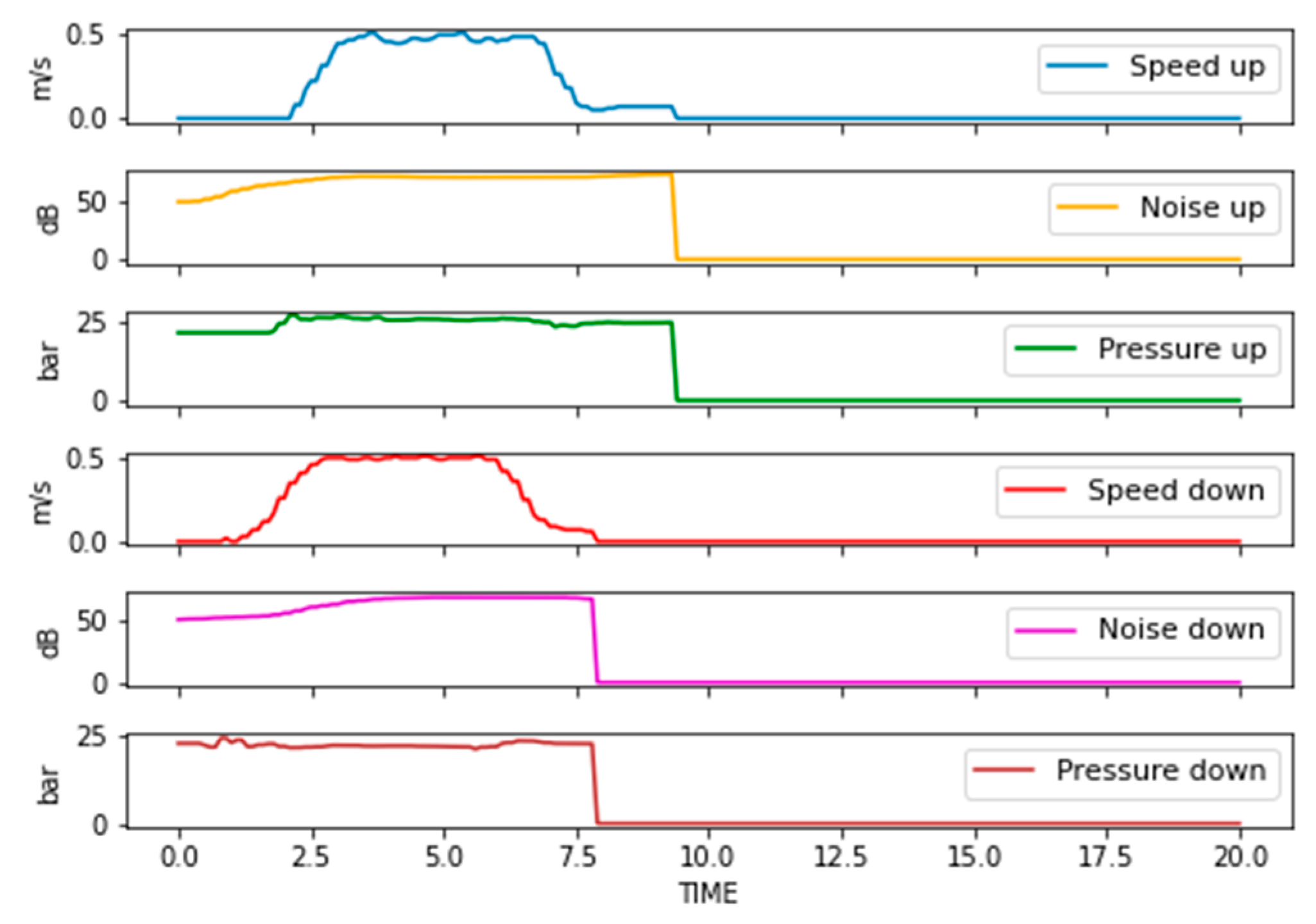
An industrial dataset was provided by KLEEMANN Greece containing historical measurements of elevator hydraulic power units (HPU). These measurements correspond to quality tests, that monitor the speed of the elevator, the developed pressure in the hydraulic unit, and noise produced during operation. The dataset contains 7200 different cases, corresponding to different client orders and employing various configurations and setups. An indicative example is shown in Figure 2.

Investigation of the provided dataset revealed that the acquired curves are not affected by the translational direction. Thus, directional information was not regarded as a classification parameter and measured curves for all direction were merged into a single dataset with $2\times 7200=14,400$ samples. On the other hand, discrepancies were observed on testing parameters, e.g., some tests last longer than others, or the HPU operated in a different speed range, etc. Such deviations occur due to the different client requirements for each individual order, and cannot be avoided; therefore, some data preprocessing is needed, as described in the following section.

3.2. Data Preprocessing

The number of captured time steps in each HPU varied from 201 to 1035, albeit most samples (ca. 80%) consisted of only 201 time-steps. Therefore, all data sequences were brought to the same length (i.e., 201 time-steps), to enable mini-batch processing. The values of speed were all in the same range [0, 0.91], thus, no treatment was necessary. Noise and pressure were in very different ranges, namely [0, 91.2] and [0, 53.98] respectively, thus, they were normalized by dividing with their maximum value.

The derived dataset was split for training (90%) and testing (10%). The sizes of the datasets involved were (samples × time steps × variables) (see

Table 1. Employed datasets for training and testing.

Dataset	Population
Training	12.960 × 201 × 3
Testing (w/o anomalies)	1.440 × 201 × 3
Testing (with anomalies)	1.440 × 201 × 3

):

3.3. Synthetic Data for Anomaly Detection

As already mentioned, a well-configured manufacturing line rarely produces measurements with anomalies. This was also the case with the provided dataset; all timeseries correspond to optimal operation. Thus, a synthetic dataset for anomaly detection testing was created to test the model and assess its performance. To prevent biasing, communications with expert technicians were conducted to establish realistic deviations and criteria for identification of sub-optimal operation. According to the technical experts, anomalies in measured timeseries should be identified by (a) deviations more than ±1.9 bar in pressure, and (b) noise values higher than 68 dB. No hard indicator could be provided for speed. Furthermore, the noise value was treated as a weak indicator, since there were samples with noise value higher than 68 dB and still treated as normal.

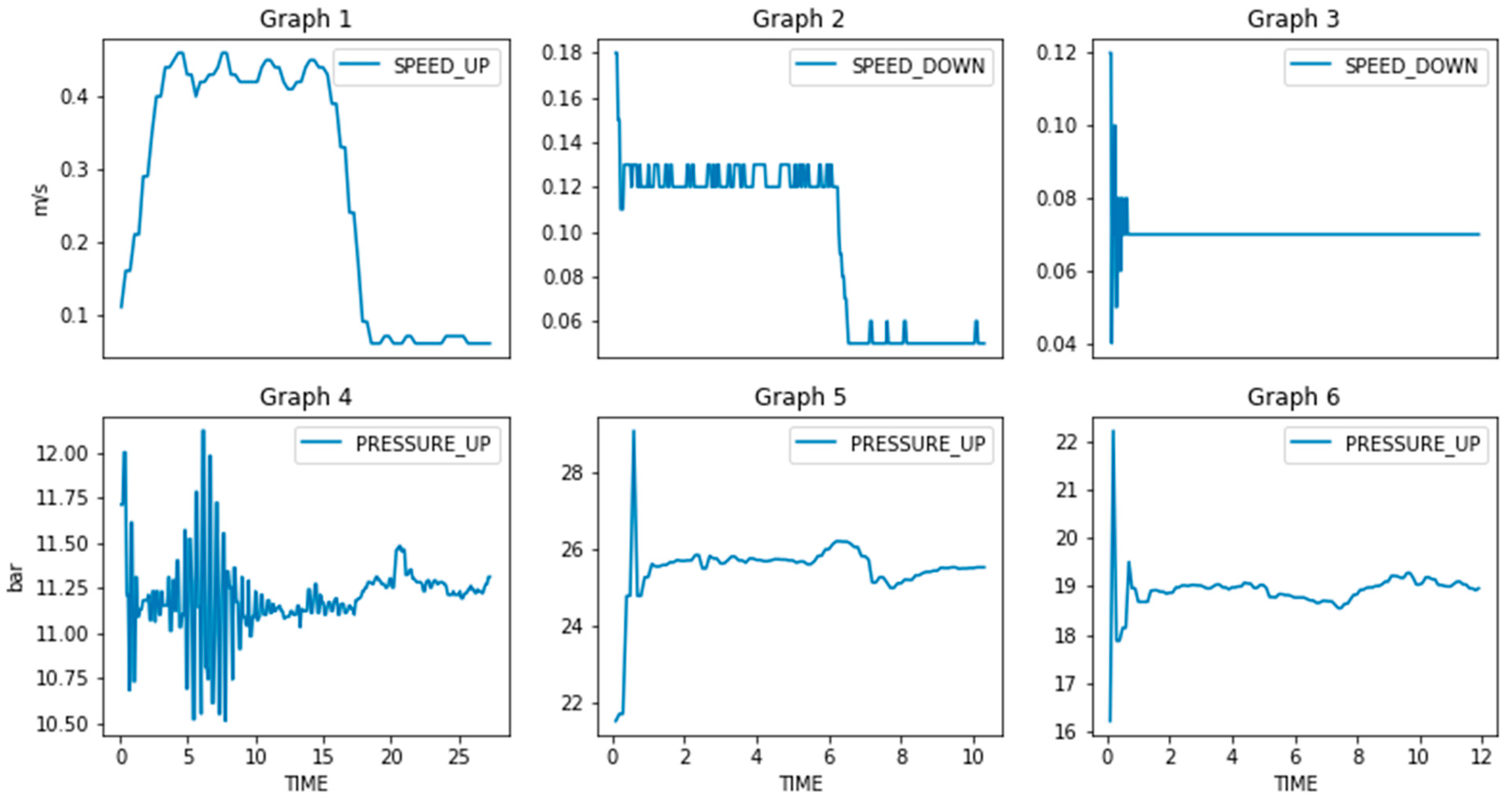
To tackle these ambiguities, the provided dataset was further explored to establish more strict and realistic thresholds; these thresholds were then exploited to induce artificial anomalies. An example is shown in Figure 3 (Graphs 1–3), where it is clear that speed is not constant but exhibits fluctuations; thus, such curves can be used to extract the fluctuation threshold, beyond which, the operation is considered sub-optimal. The same applies for pressure (Graphs 4–6). Following this approach, the following factors were accounted for during generation of artificial anomalies:

• Duration. Point anomalies seem to be of minor importance, at least in the beginning of testing. Hence, anomalies of finite duration were chosen randomly with a minimum of 10 time-steps.
• Magnitude. Both positive and negative deviations were induced, with addition or subtraction of random numbers with magnitude: [1.6 bar, 2.6 bar] for pressure, [1 dB, 4 dB] for noise and [5, 20]% of the maximum speed value of the curve for speed.
• Location. Location of the anomalies was chosen randomly between the timesteps that the test is performed (operational values > 0).

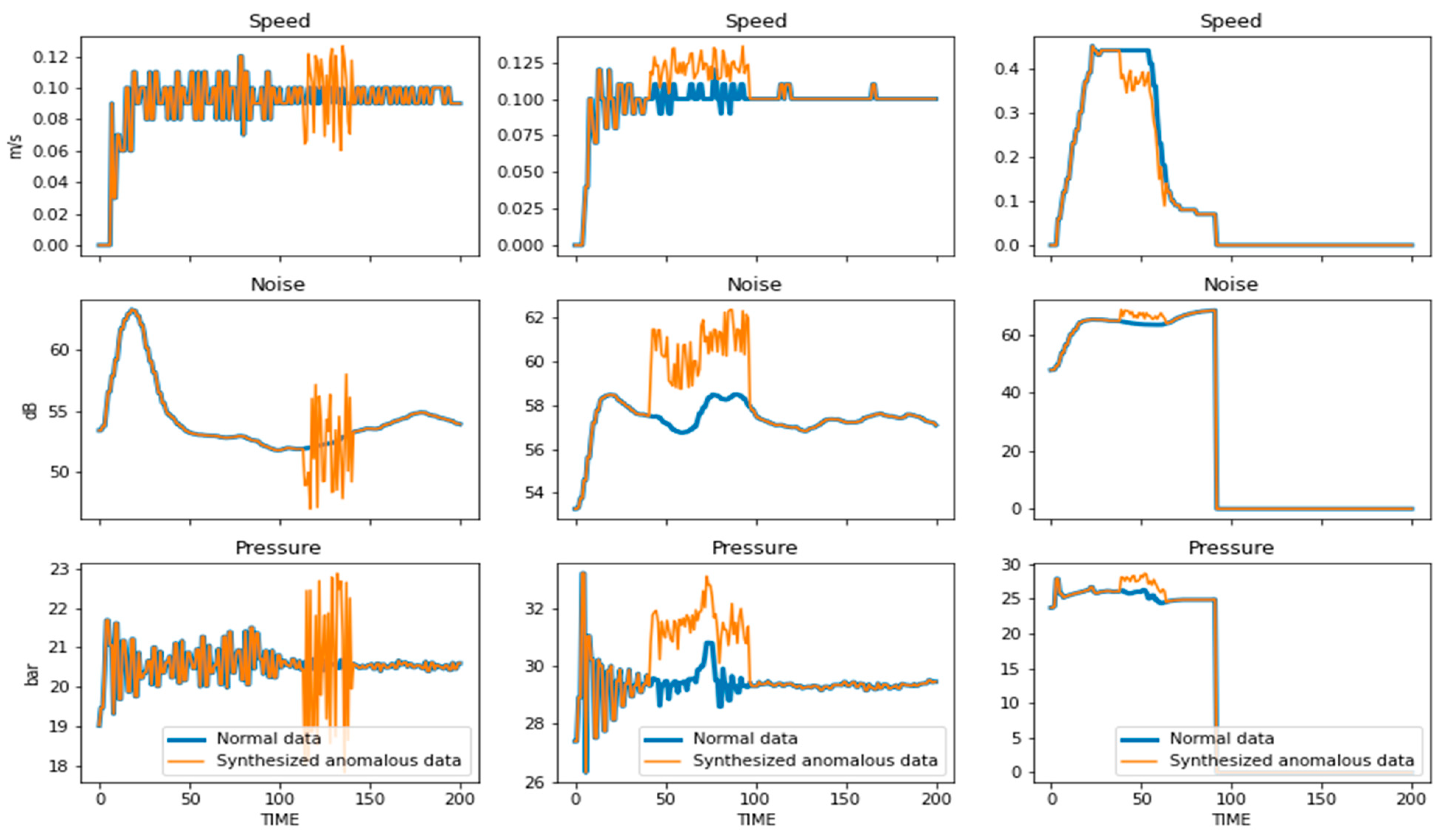
To create the synthetic dataset for anomaly detection for testing, each measured curve of the normal testing dataset was processed. Therefore, each curve in the testing dataset for anomalous detection is the counterpart of a curve which includes anomalies in the normal testing dataset. Examples of normal and synthetic curve-pairs including artificial anomalies are shown in Figure 4.

3.4. Description of the AE Architectures

To acquire the most appropriate AE for AD in this industrial dataset, three different AE architectures were considered, namely ANN-, LSTM- and CNN-based AEs. Thus, some popular architectures found in literature were explored and assessed using the training and testing datasets described.

ANN-based AE. The first implementation was an ANN-based AE. It consisted of 10 fully connected (dense) layers, a layer that flattens the matrix and a reshape layer in the decoding operation that transforms the vector back to a matrix. In particular, the architecture is as follows: Input (128-64-32)-flatten-1024-latent space (128)-(1024-6432)-reshape (64-128)-output. For all hidden layers ReLU activation function was used.

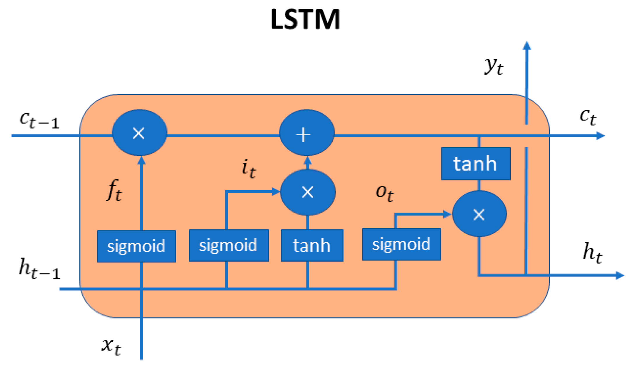
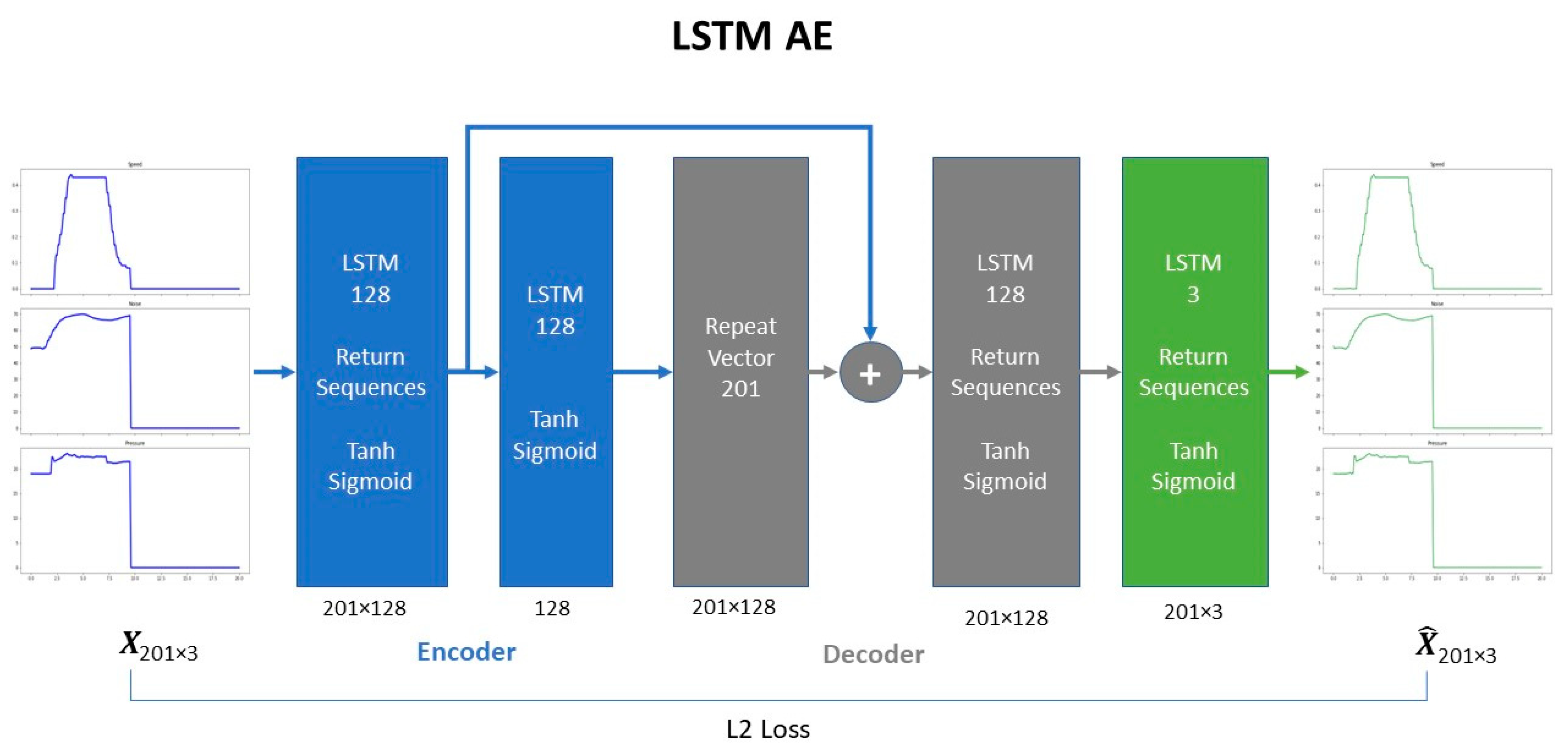
LSTM-based AE. The LSTM-based AE is a shallower network compared to the previous one. It consists of 4 LSTM layers, a layer that repeats the vector in the corresponding timesteps and a skip connection layer. Hyperbolic tangent and sigmoid activation functions were used in LSTM units for the input and the recurrent state respectively. Skip-connections were employed in the stacked LSTM layers, following the practice of [16,17,18], to boost model’s reconstruction performance. The architecture is shown in Figure 5.

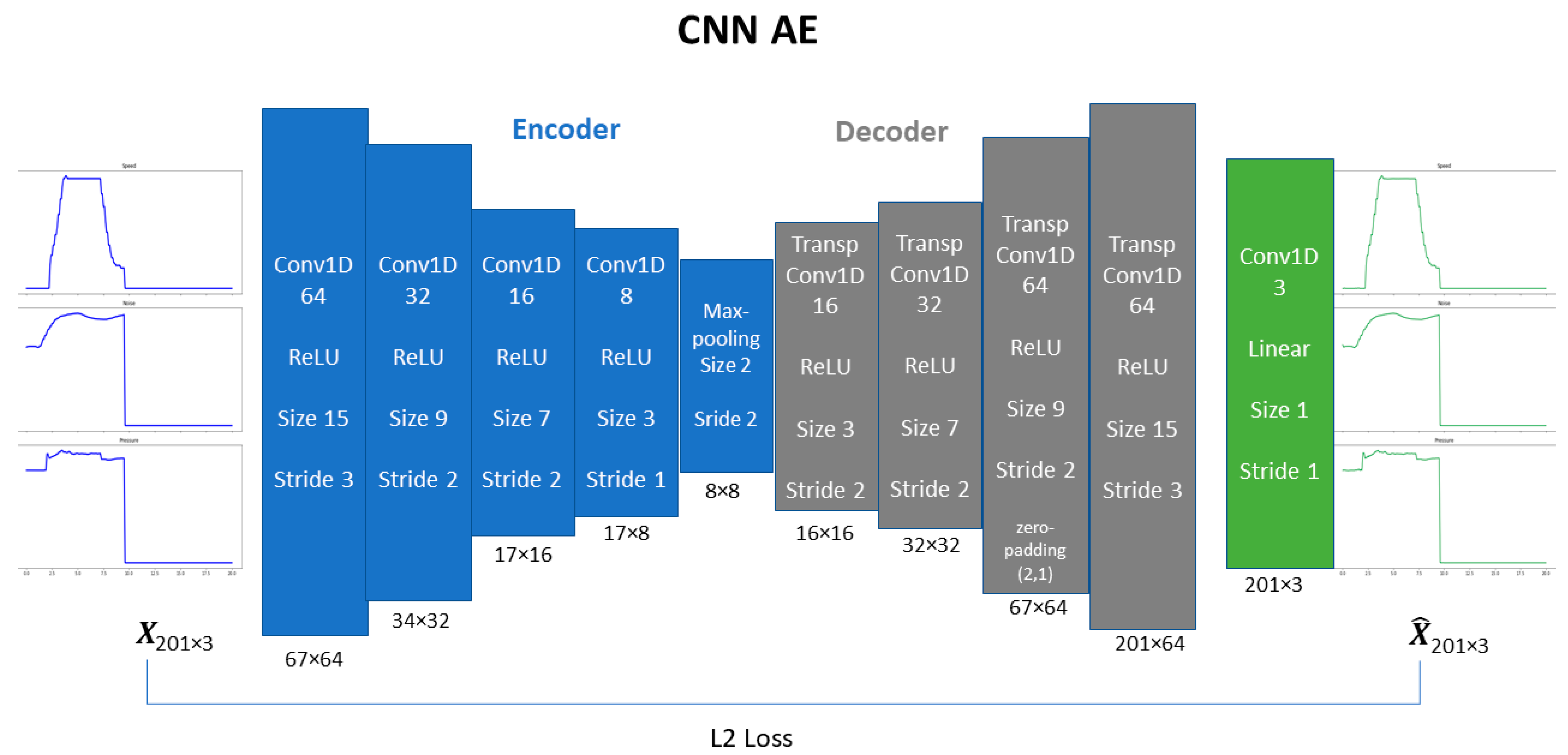
CNN-based AE. The CNN-based AE consists of convolutions, transpose convolutions and pooling operation. Convolutions and pooling operation were part of the encoding process while transpose convolutions [19] were used to perform up-sampling during decoding. Convolutional and transpose convolutional layers employed the “same-padding” method, so that the size of the output matched the size of input. ReLU was used as the activation function. The complete architecture is presented in Figure 6.

3.5. Results

All the experiments were conducted on a custom-built workstation to accommodate the computational needs of OPTIMAI; the workstation was equipped with an Intel Core i9-11900KF @ 3.5 GHz CPU, 16 GB RAM and NVIDIA GeForce RTX 3080 Ti with 12 GB of GDDR6X memory, running on Windows 10 Pro. The proposed AEs were implemented in Python 3.8.3, with the Keras API framework of TensorFlow 2.0 [20].

The dataset was split by random selection for training (90%, 12,960 records) and testing (10%, 1440 records) so as to acquire a larger representative training dataset that will assist the network to learn the variety of operational values [21]. A smaller testing dataset is produced considering both synthetic anomalies and normal cases.

The L2 loss was chosen as the training cost function. In all experiments, both 5-fold and 10-fold cross validation were used, with the hold-out group of data being exploited as a validation dataset during training. The early stopping setup of Keras was used to avoid overfitting. As shown in

Table 2. Computational characteristics for each proposed architecture.

AE	Training Time (s)	Epochs	Total Parameters	Threshold	Accuracy	Precision	Recall
ANN-based	81	122	13,465,155	0.0063	84.79	91.27	76.94
LSTM-based	677	91	332,336	0.00048	91.38	96.05	86.31
CNN-based	101	99	109,611	0.00514	94.09	97.10	90.90

, there was a considerable difference in the running times and number of epochs required for AEs to converge. The ANN-based AE was the fastest model to train despite it involved significantly more parameters than the others. CNN-based AE on the other hand, combines both computational efficiency and low training time.

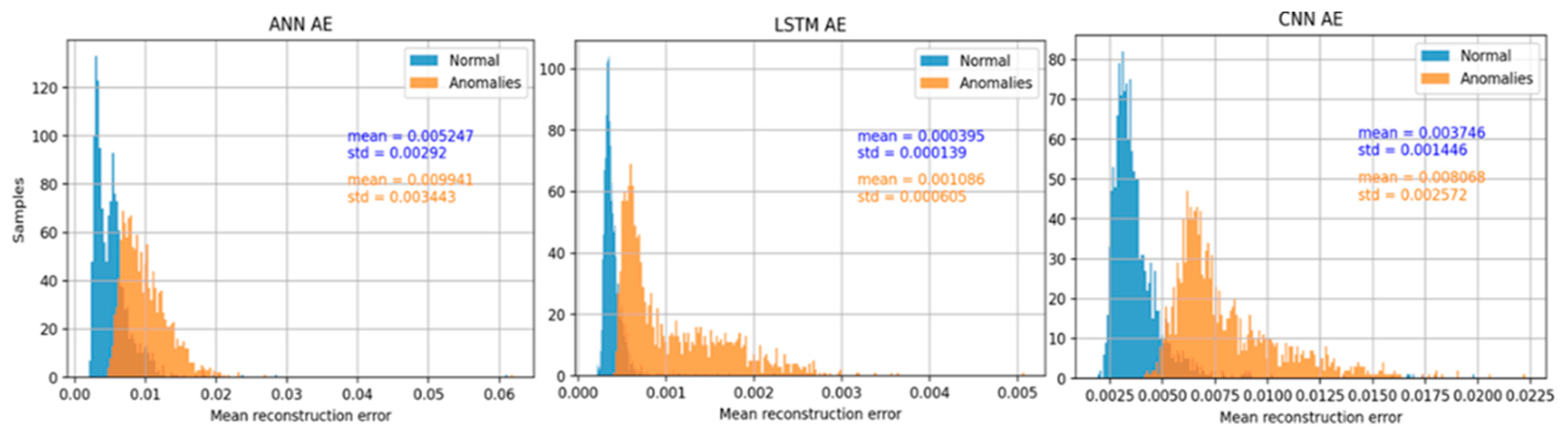
To determine the most suitable AE type, one critical parameter needs to be considered: the classification threshold. To determine the classification threshold of signals as normal or anomalous, the mean reconstruction error values were investigated. Both the MSE and MAE metrics were considered, but the MSE curves was prone to outliers; thus, the classification threshold was selected based on MAE. The distribution of MAE for both normal and synthetic samples in the data is presented in Figure 7. An ideal model would perfectly reconstruct its input; thus, no overlap (zero error) should be observed in the diagrams; or equivalently, the higher the overlap the worse the performance.

Optimal performance was achieved by setting the threshold to 0.0063, 0.00048, and 0.00514 for the ANN-based, the LSTM-based and the CNN-based AEs, respectively.

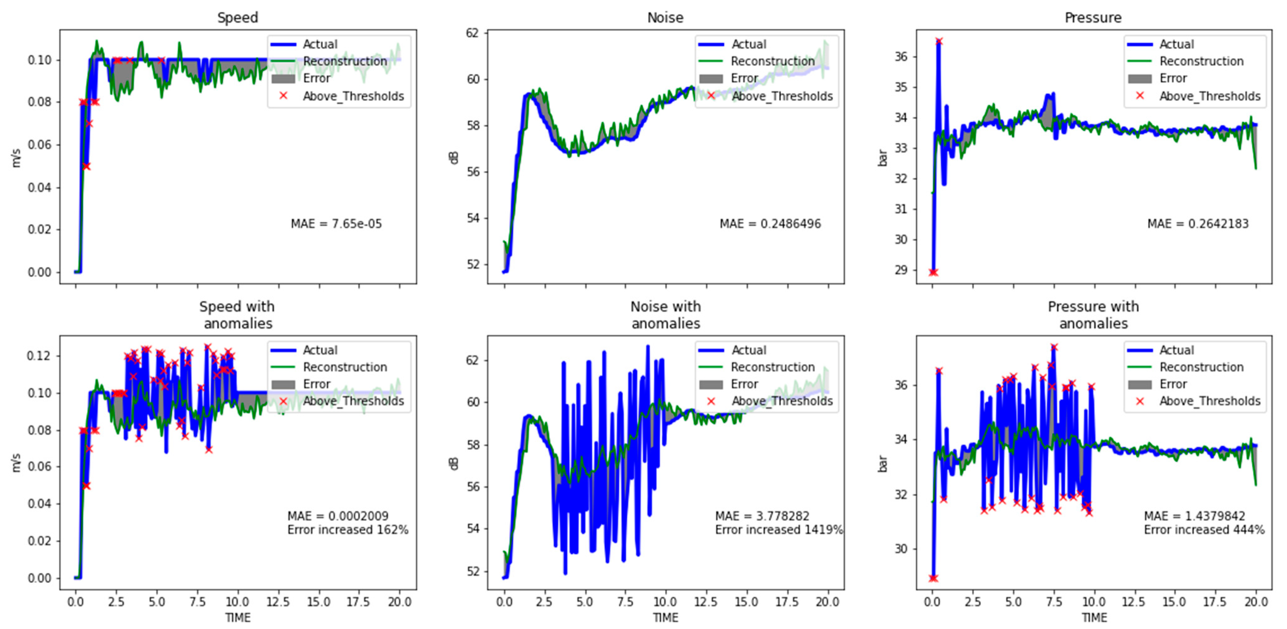
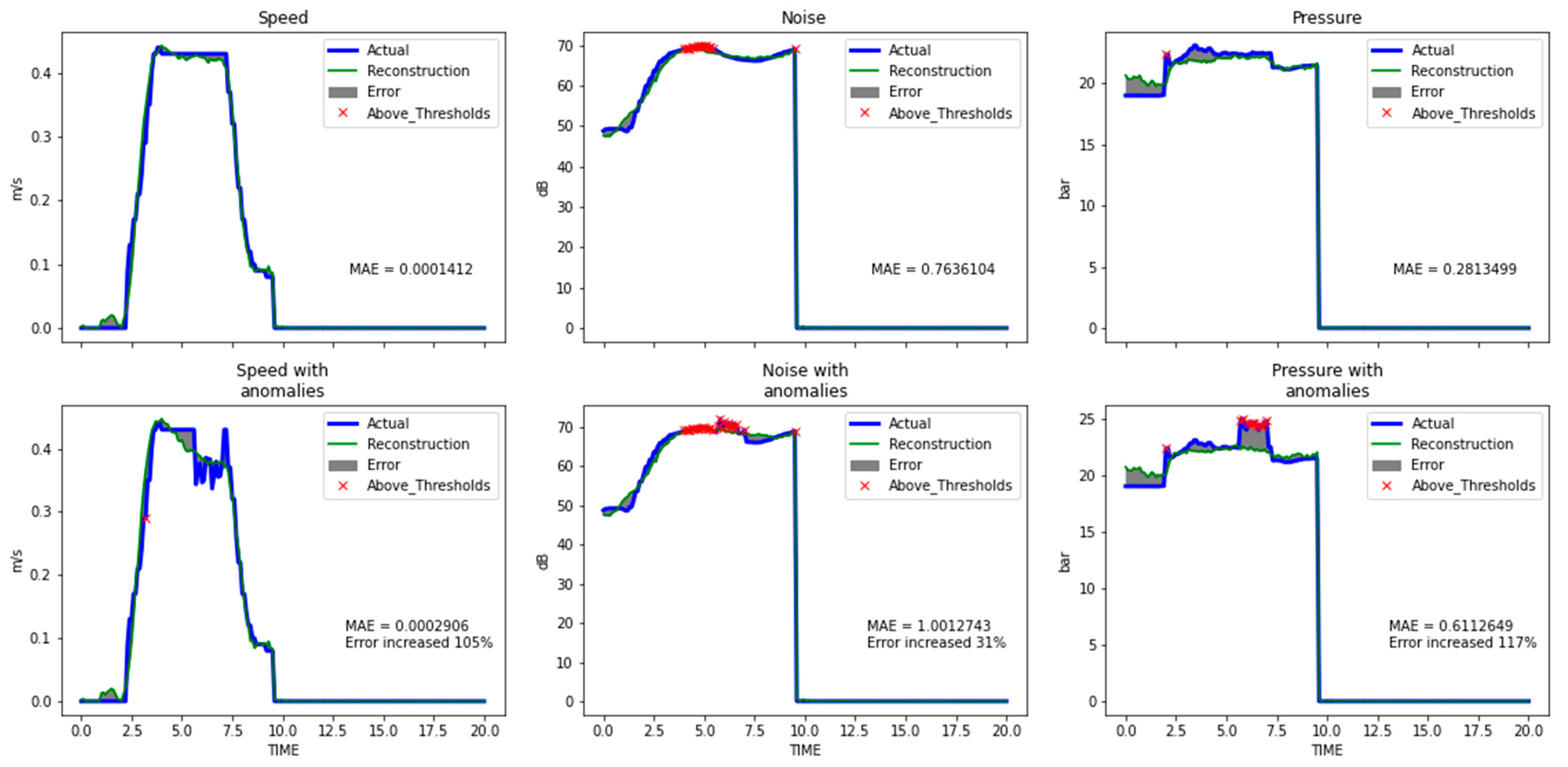
The CNN-based AE achieved the highest scores according to the classification metrics (see Table 2). Its reconstruction capabilities are presented for two types of anomalies in Figure 8 and Figure 9, with the corresponding MAE for both normal- anomalous pairs. Oscillations (Figure 8) produced higher ΜAΕ errors than dips/rises failures (Figure 9). However, further research is needed regarding localization using DL methods.

All three examined AEs architectures demonstrated enhanced anomaly detection capabilities by producing a higher reconstruction error when fed with data including anomalies. According to the provided results, LSTM-based AE achieved the lowest reconstruction error for both cases of input data (normal or synthetic with artificial anomalies) which reveals that CNN-based AEs present higher sensitivity to anomalies. In terms of classification capability, the LSTM-based AE provided worse classification metrics than those achieved by the CNN-based AE, according to the MAE distribution graphs and the observed overlap, which also limited the range for the selection of the classification threshold. Overall, it emerges that the CNN-based AE shows better performance with regard to accuracy, also requiring less training time due to the reduced number of parameters.

4. Conclusions

To tackle the absence of anomalies in the data that is a common problem of real industrial datasets, a simple methodology of inducing anomalies based on expert’s knowledge and data analysis was deployed. The AE based on 1DCNN layers outperformed in terms of classification accuracy, both LSTM-based and ANN-based AE. In addition, the ability of the CNN layers to share weights reduced the parameters-depth analogy of the proposed model and resulted in fast training times. The model achieved distinction of normal data and data including anomalies with 94% accuracy in an industrial dataset enhanced with artificial anomalies. Moreover, this work presented a methodology for inducing artificial anomalies, in order to generate samples that deviate from the normal operational thresholds of the examined industrial dataset.

Regarding the limitations with our approach, the possibility that the artificial dataset might not be representative for all possible outcomes including anomalies, is one of them. Thus, the classification threshold that selected with our approach can be considered optimal just for this test dataset. For future work, the consideration of real anomalies and the examination of other methodologies in classification threshold estimation, are essential.