
A Review of Wave-to-Wire Models for Wave Energy Converters


Centre for Ocean Energy Research, Maynooth University, Maynooth, Co. Kildare, Ireland
*
Author to whom correspondence should be addressed.
Energies 2016, 9(7), 506; https://doi.org/10.3390/en9070506
Submission received: 23 March 2016
/
Revised: 15 June 2016
/
Accepted: 17 June 2016
/
Published: 30 June 2016
Abstract
:Control of wave energy converters (WECs) has been very often limited to hydrodynamic control to absorb the maximum energy possible from ocean waves. This generally ignores or significantly simplifies the performance of real power take-off (PTO) systems. However, including all the required dynamics and constraints in the control problem may considerably vary the control strategy and the power output. Therefore, this paper considers the incorporation into the model of all the conversion stages from ocean waves to the electricity network, referred to as wave-to-wire (W2W) models, and identifies the necessary components and their dynamics and constraints, including grid constraints. In addition, the paper identifies different control inputs for the different components of the PTO system and how these inputs are articulated to the dynamics of the system. Examples of pneumatic, hydraulic, mechanical or magnetic transmission systems driving a rotary electrical generator, and linear electric generators are provided.
1. Introduction
The increasing penetration of renewable energy sources into the power grid, especially wind and solar energy, poses a daunting challenge to both renewable energy plants and the electricity network, due to the variability of the renewable sources and the rigorous restrictions of the network.
Wave energy is also expected to contribute to the future power supply. However, if wave energy is to be a serious competitor among the renewable energy sources, first, the generated energy must fulfil the requirements imposed by the network, and second, power flow between waves and the grid needs to be maximised.
Due to the reciprocating motion induced by ocean waves and the variability of the resource, power produced by wave energy converters (WECs) is even more uneven than other renewable sources, as illustrated in Figure 1. For example, most thermal (and hydro)power plants can produce the nominal output power specified by the rated generator capacity, where the generator performs close to nominal speed. However, in wave energy the high variability of the resource induces extreme variations between peak and average values, which requires the rated power (nominal power) of the generator to be considerably higher than the typical average power value. The difference between the highly-variable resource and the severe restrictions of the grid suggests that control is crucial to maximise power output within the limits stipulated on the grid code.
Apart from the grid restrictions, each of the components used in the power conversion can add constraints to the conversion process, such as force, displacement or speed limitations. Besides, these components are designed to efficiently perform close to nominal values, but lose performance as soon as operation conditions move away from these nominal values. Consequently, a simulation model that includes all the necessary components for the energy conversion, and its dynamics, is imperative to design the optimal control strategy and maximise the power output.
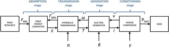
The path from ocean waves to the grid can, maximally, be divided into six steps, as shown in Figure 2. The initial and final stages refer to the wave resource and the grid, respectively, while the intermediate four stages indicate the different intermediate conversion stages. The focus of the present paper is on the control requirements of these intermediate conversion stages, so the wave resource assessment is beyond the scope of the paper. However, several methods for resource assessment have been suggested in the literature [2,3,4,5], which can be incorporated prior to the articulation of the device.
Figure 2 illustrates a power take-off (PTO) system with the four conversion stages highlighting the potential control inputs that includes a hydraulic transmission system:
- Absorption stage
- Transmission stage
- Generation stage
- Conditioning stage
The absorption stage comprises the conversion of wave motion into oscillating motion of the WEC. This absorbed energy is transmitted into hydraulic energy in the transmission stage and converted into electrical energy in the generation stage. Finally, the outgoing power signal is adapted to be delivered into the grid in the conditioning stage. However, the hydraulic system illustrated in Figure 2 can be replaced by a mechanical or magnetic transmission system, preserving the four-conversion-stage system (absorption-transmission-generation-conditioning). In some particular cases, known as direct conversion, the WEC is directly connected to the electrical generator using a linear generator, in which case, the transmission stage is eliminated resulting in a three-conversion-stage system (absorption-generation-conditioning). Note that the distinction between energy absorption and generation is made intentionally, where absorption refers to the mechanical energy absorbed from the ocean waves and generation to the electrical energy generated through the power take-off system.
Models that incorporate all these stages from waves to the grid are known in the literature as wave-to-wire (W2W) models.
1.1. Existing Wave-to-Wire Models
A number of W2W models have been presented in the literature for different types of WECs: overtopping converters [6], oscillating water columns (OWCs) [7], or wave-activated converters with different PTO strategies, e.g., hydraulic [8,9,10,11,12,13], mechanical [1,14], magnetic [13], or linear generators [15,16].
The level of detail at each stage of the power train can vary from model to model, usually depending on the expertise of the authoring research group and the focus of the model. Table 1 presents a summary of a critical comparative review. It is, however, important to note that the evaluation of the studies found in the literature is made with respect to the control requirements, which may not be consistent with the requirements of the original studies.
The absorption stage, i.e., wave and WEC hydrodynamic interaction, is modelled by means of the fully linear method in most cases, which is computationally appealing, but may not be accurate enough for control requirements, as further discussed in Section 2. Among the different W2W models found in the literature, only [11,12] include losses or nonlinear forces are included in the hydrodynamic model, incorporating viscous losses and nonlinear restoring force, respectively.
Different technologies have been suggested for the transmission stage, with the hydraulic system as the most utilised one. Hydraulic systems are comprised of several different components, which require a great level of detail in the modelling in order to accurately predict their dynamic behaviour. Dynamics of the hydraulic cylinder and motor are considerably simplified in general, ignoring different losses and constraints. Josset [8] considers only the compressibility effect of the fluid in the cylinder chambers, [10] includes constant losses in the motor, [11] takes into account dynamic losses in the motor and [13] includes constant efficiency in the cylinder and dynamic losses in the motor, validating simulated results against experiments. Dynamic models for hydraulic accumulators are reasonable in most of the studies, while the dynamics of the hydraulic valves are only considered in [13].
In relation to the generation stage, dynamics of rotary electric generators have been incorporated in [1,10,12,13,14], although the transient behaviour is ignored in [13]. The other studies utilise constant torque and/or efficiency values to emulate the generator. However, in the case of W2W models based on direct conversion using linear generators, dynamics of the electric generators are generally included, as shown in [15,16], although [16] simplifies the analysis by assuming no field weakening.
The conditioning stage needs only to be included in the case where a variable-speed generator is employed. Dynamic models for power converters are included in [1,14,15,16].
References [6,7] are also defined at the beginning of this section as W2W models, but since they do not study wave-activated WECs, they do not fit in the classification presented in this section. However, both include dynamic models for the rotary electric generator and power converters, including experimental analysis in the case of [7].
Finally, the inclusion of the electricity network in W2W models is analysed. Garcia Rosa [10] studies voltage and frequency fluctuations of the outgoing power signal, [12] includes a power flow solver for the array of WECs, and [1] studies rapid fluctuations in grid voltage (referred to as flicker), reactive power and harmonic corrections and fault ride-through response.
Therefore, to date and to the best knowledge of the authors, no published wave-to-wire model captures all the main characteristics required to allow the design of a complete wave-to-wire control system, which should include:
- Balanced parsimonious models for each stage of the drive train (including nonlinearities where required);
- Consideration of all possible control inputs at the various stages in the drive train;
- Articulation of constraints, energy losses and efficiency curves for each component;
- Specification of physical constraints for each component, e.g., displacement, velocity and force (for mechanical components), pressure (for hydraulic components), current, voltage (for electrical components) and power specification (at all levels). The specification of electrical grid constraints, including power quality measures, is also important, as appropriate.
1.2. The Control Problem
The purpose of a control strategy is to make the controlled system behave in a manner so that different components of the system meet optimal performance specifications. Such a control strategy requires control inputs which can be modified to optimise the performance goal.
Since a similar system to a wave energy converter is a wind turbine, due to the variability of the resource and the components employed in the system, it provides a useful starting point for control analysis. In wind turbines with variable-speed generators, the generator torque is used to control the rotor speed to maximize power extraction, when operating below the rated power of the generator. Above the rated power, pitch-control is used, manipulating the angle of attack of the blades, to maintain constant output power.
With respect to wave energy converters, Figure 2 illustrates three potential control inputs (α, β and γ), each of them applied to a different conversion stage. In general only one of these inputs is required for control, but a combination of the different inputs may be favourable to optimize the efficiency of the different components in the system, as mentioned in [17]. Similarly, additional control strategies, such as velocity- or/and voltage-control, are sometimes added to the previously mentioned torque- and pitch-control in wind turbines.
The control problem in wave energy is unfortunately as necessary as it is complex. Due to the non-causal nature of the optimal control problem, future knowledge of the free-surface elevation or excitation force is required to predict the optimal PTO force to be applied. Thus, wave forecasting is essential, which can be performed using up-wave measurements [18] or modelling at the device location [19].
Different constraints, non-ideal efficiency or nonlinear dynamics of the system, which strongly affect the control strategy, make the control problem hard to solve using conventional control approaches. Several studies in the literature have analysed the need to incorporate constraints, non-ideal efficiency or nonlinear dynamics into the control problem:
Therefore, powerful algorithms, such as model predictive control (MPC) [23] or pseudo-spectral methods [24], have been suggested to address the control problem in wave energy converters.
However, to the best knowledge of the authors, none of the studies in the literature has included all the required dynamics and constraints in the control problem formulation. An (understandable) approach to the control of the full wave-to-wire system is to individually control mechanical, hydraulic and electrical subsystems, attempting to keep individual components operating optimally including, for example, control of the hydraulic system to a fixed pressure setpoint and the generator to a fixed speed. However, such individual control objectives typically conflict with each other and also place significant constraints on the maximisation of hydrodynamic power capture.
The degree to which each individually controlled subsystem must compromise to achieve overall system optimality can only be accurately achieved with a complete wave-to-wire model and, indeed, the area of global control of the complete wave-to-wire system is a pertinent topic for research.
The aim of this paper is to identify all the necessary components, and associated parameters, of the power train, to determine how best structure the control system, and how the available control inputs are articulated to the dynamics of the system.
2. Absorption Stage
In the conversion from wave motion into oscillating motion of the absorber (where absorber refers to the the part of the WEC that absorbs energy from the ocean waves, i.e., the internal water surface (IWS) in an OWC converter modelled as a piston, the float in a heaving point absorber or the flap in an oscillating converter), different forces can be included. Newton’s second law is used to specify the governing equation of a WEC as follows:
where is the mass matrix and n the number of degrees of freedom (DoF) of the system, the position vector of the WEC and , and are vectors describing the hydrodynamic force, the force applied by the PTO system and any other force impacting the problem, such as mooring forces or the force induced by the wind, respectively.
The hydrodynamic force () can, in turn, be divided into different forces, which in the simplest version is composed of three parts: the hydrostatic force (also known as the restoring force), the wave excitation force and the radiation force. Equation (1) can be then represented by means of the Cummins equation [25] as follows:
where is the matrix describing the hydrostatic stiffness, η the free-surface elevation, the infinite frequency added-mass matrix and and are, respectively, the excitation and radiation impulse response functions (IRFs). The elements of the matrix of the radiation IRFs are continuous functions in and zero for , where .
The vector of the PTO forces is given as , where is a constant matrix, known as configuration matrix, that allows for the combination of the different oscillation modes to absorb energy [26,27]. The number of PTO forces (m) is, in general, lower than the number of oscillation modes (). Hence, in the case of a single-body heaving point absorber device referenced to the seabed, there is a single DoF and a single PTO force, so . In contrast, in the case of a self-reacting two-body system constrained to only oscillate in heave, two degrees of freedom and a single PTO force exist, so the configuration matrix is given as follows:
which shows that the PTO force acts with the same magnitude but opposite direction on each body of the two-body system.
The vast majority of hydrodynamic models are based on linear assumptions, where the hydrodynamic parameters (, , , or ) are identified using the well-known boundary element method (BEM) implemented in open source or commercial codes, such as NEMOH [28] or WAMIT [29]. NEMOH and WAMIT solve the radiation/diffraction problems for the study of the interaction between offshore structures and ocean waves and are based on the tree-dimensional panel method. The linear approximation assumes small waves, small motion amplitudes, constant hydrodynamic coefficients and no viscous effects. However, the small motion assumption is challenged, since the objective is to exaggerate the WEC motion to maximise power capture.
Therefore, nonlinear or higher-order hydrodynamic effects may be included in the model, such as nonlinear hydrostatic force [30,31], nonlinear FK forces [32], higher-order terms of the radiation and diffraction forces [33] or viscous a drag force [34].
Some studies in the literature present fully linear hydrodynamic models, validated against wave tank experiments [35,36,37]. However, conditions under which wave tank experiments are carried out should be taken into account, since linear models may appear to be accurate under some conditions, but lose accuracy in the case of more significant motions. The control force itself can therefore be a source of nonlinear effects, as demonstrated in [20].
Hence, hydrodynamic models that include nonlinear effects have been suggested in the literature. Penalba [38] classifies nonlinear BEM models into three groups: partially-, weakly- and fully-nonlinear models. The partially nonlinear method can be described as an extension of the linear model, where the hydrodynamic force () can be decomposed into six terms to include nonlinear and higher-order effects:
where , and are the FK force (including static and dynamic FK forces), the radiation force and the diffraction force vectors, respectively, and indexes and denote first- and second-order solutions.
The impact of viscous losses can also be significant in some cases. Bhinder [34,39] study the impact of viscous effects in a floating heaving WEC and a surging flap, respectively. A possibility for the improvement of linear models is to account for viscous effects via an additional quadratic damping term. The intensity of this additional damping depends on the so-called drag coefficient (), which needs to be estimated using experimental tests or CFD simulations. The viscous force is incorporated into the linear model as an additional force, following the semi-empirical formulation based on the Morison equation [40]:
where is the water density and and are the positive constant diagonal matrices describing the drag coefficient and the cross-sectional area of each of the oscillation modes of the absorber.
These nonlinear effects and losses, nonetheless, may not be always necessary. Depending on the type of WEC and its motion characteristics, certain nonlinear effects may be significant or negligible, and a cautious choice needs to be made in relation to the incorporation of nonlinear effects, since significant computational costs may be added to the simulation and/or control calculations. Penalba [38] reports the relevance of different nonlinear forces for various types of devices.
3. Transmission Stage
The conversion from wave-induced mechanical motion into useful energy can be carried out using different technologies. The main challenge for the technologies to be implemented in this transmission stage is to reliably and efficiently convert the power absorbed by the WEC, dealing with the extreme variations between maximum power peaks and average power flow (which can be higher than a factor of 10).
3.1. Pneumatic Transmission
Pneumatic conversion by means of air-turbines is implemented in a significant category of WECs, where a fixed (e.g., the LIMPET shoreline plant [41], the PICO power plant [42], the Mutriku wave power plant [43] or the recently built Yongsoo plant [44]) or floating structure (e.g., the Backward Bent Duct Buoy (BBDB) converter [45,46], the Mighty Whale concept [47] or the Oceanlinx converter [44]) is utilised to trap the air between the free-surface and an air turbine.
The structure is open to the sea at its lower end, partially filling the inner chamber with sea water. The oscillations of the water column in the chamber (illustrated with dotted line in Figure 3), due to the action of the waves outside the structure, pressurises and depressurises the air trapped in the chamber, forcing it to flow through the air turbine located at the upper end of the structure. Figure 3 illustrates the principles of the OWC devices, representing the wave pressure on the air-water interface and the air-flow through the turbine due to the displacement of the water-column.
Falcão [44] gives a good overview of OWC devices, including the different existing OWC technologies and turbine configurations, modelling techniques and control strategies. Two main modelling aspects specific to OWCs include the thermodynamics of the air flow in the chamber, and the air turbine model. In addition, the hydrodynamic model of OWCs includes some unique aspects when modelling the IWS. Hydrodynamics modelling, thermodynamics in the chamber and air-turbines for OWC converters are described in the following subsections.
It is important to note that, although the different aspects (hydrodynamics, thermodynamics and air-turbines) are very often described and modelled individually and independently, they are actually interdependent [7,48,49,50,51].
3.1.1. Hydrodynamics for OWC Converters
Unique aspects pertain to the hydrodynamic wave-structure interaction for OWCs. Evans [52] studies the hydrodynamic performance of OWC devices based on linear water wave theory, using the so-called piston-model approach, where the air-water interface is assumed to behave as a horizontal piston, as shown in Figure 3 by the dashed horizontal line where the wave pressure is applied. A more accurate model suggested in [53] and generalised in [54], where a spatially uniform pressure distribution is assumed on the free surface in the chamber.
The advantage of the piston-model is that the interaction between waves and the WEC can be analysed by using the well-known wave-structure interaction theory [55,56]. Therefore, hydrodynamic parameters for OWC devices modelled using the piston-model approach can be obtained using the BEM codes mentioned in Section 2. Hence, the most widely-used time-domain hydrodynamic model structure, based on the Cummins equation and presented in Equation (2), is also appropriate for OWC devices, as far as the piston model is an acceptable representation of the inner free-surface. However, a new term, which represents the effect of the pressure between the chamber and the atmosphere that induces body oscillations, needs to be included. Such term is referred to as pressure force () and is given as follows,
where is the area of the piston that represents the free surface in the chamber and the pressure difference () between the pressure in the chamber () and the atmospheric pressure ().
The fixed OWC device can be modelled as a single-body converter, where the imaginary piston that represents the inner free-surface is the absorber. In the case of floating OWC devices, the converter needs to be considered as a multi-body system comprised of the floating structure (floater) and the imaginary piston. If both bodies are constrained to oscillate in heave only, the floating OWC becomes a two-body system [49,57] and the configuration matrix shown in Equation (3) can be used.
3.1.2. Thermodynamics in the Chamber
Pressure oscillations in the OWC chamber determine the evolution of the air mass in the chamber and the air flow through the turbine, which are studied by using thermodynamic relations. The compressibility effect in the chamber is important in OWC devices, especially in full-size OWC converters [44], which is very often modelled utilizing a simple isentropic relationship between air pressure and density () [58,59,60],
where is the specific heat ratio of the air (). The assumption of an isentropic and adiabatic process in the chamber is reasonable, since the heat exchange in the chamber during a wave cycle is considered to be small [61].
Therefore, pressure in the chamber can be given as follows [62]:
where is the air volume, the density of the air at atmospheric pressure, is the air mass flow through the turbine and .
The air volume in the chamber is proportional to the displacement of the water column, and the variation of the air volume is proportional to the velocity of the water column. Air mass flows in (inhalation) and out (exhalation) of the chamber through the air turbine. When , air in the chamber is pressurized and air is exhaled from the chamber. In contrast, when , air is depressurised in the chamber, and air is inhaled into the chamber.
3.1.3. Air Turbines
The pressure difference created in the chamber by the ocean waves drives the air turbine located at the top of the OWC structure. The most widely used method for modelling air turbines is based on dimensional analysis [51,61,63,64], where the dimensionless flow and dimensionless power are given as a function of the dimensionless pressure head [65],
where
and , and are the pressure drop across the turbine, the rotational speed and diameter of the turbine, respectively, is the reference density, measured at stagnation inlet conditions (which is different for inhalation and exhalation), the turbine power output and Φ, Ψ and Π are the dimensionless flow rate, pressure head and the aerodynamic torque or turbine power output, respectively. However, it should be noted that under the normal operating conditions the Reynolds and Mach numbers effects can be ignored and the air flow through the turbine is considered to be incompressible.
Different options to model the air turbine have been presented in the literature [44,66], such as turbine induced damping where, in general, a linear relationship between chamber pressure and air mass flow is used for Wells turbines, via Equation (13), and a nonlinear relation for self-rectifying impulse turbines, via Equation (14),
where the constants and depend only on the turbine geometry if Reynolds and Mach numbers effects are neglected, and typically . Following Equations (13) and (14), Equations (15) and (16) can be derived for Wells and impulse turbines, respectively, which show the influence of the turbine rotational speed on the OWC hydrodynamics when using Wells turbines, and the independence of the hydrodynamics and the turbine rotational speed, in the case of impulse turbines.
where for a quadratic impulse turbine.
Although conventional turbines can be used in OWC devices, the reciprocating motion of ocean waves makes necessary a rectifying system, since unidirectional turbines have been proven to be impractical in large OWC plants [44,66]. Therefore, different self-rectifying air turbines were developed for OWC devices, which can be divided into two main turbine categories: Wells turbines [67] and impulse turbines [68], shown in Figure 4a,b, respectively. Other turbine configurations have been also suggested such as the modified Wells turbines [69], the Dennis-Auld turbine [70,71] or the recently developed biradial turbine [72]. Falcão [66] presents a good overview of the different air turbine configurations for OWC converters and their main characteristics.
A comparison between Wells, axial-impulse and biradial turbines is shown in Figure 5, where the efficiency of the different turbines is shown against flow rate. The operational flow range of axial-flow impulse turbines is wider compared to the range of Wells turbines, since the efficiency of Wells turbines sharply drops when stalling occurs at rotor blades [73]. The efficiency of the turbine is given as follows [51]:
where is the power extracted by the turbine, is the torque applied on the turbine, the flow through the turbine and the incident pneumatic power.
In order to build an accurate wave-to-wire model, the time-variant evaluation of the flow through the turbine and the mechanical torque applied to the turbine is essential. Once the dimensionless coefficients presented in Equations (10)–(12) are identified for the turbine, the flow and the torque are derived from Equations (10) and (12), respectively [51,74],
where is assumed to be the atmospheric density in a first approximation.
The modelling of the turbine/generator set is also essential for a wave-to-wire model, which is presented in Equation (50) in Section 4.1 generalised for any transmission system.
The efficiency of the turbine can be increased considerably through the use of an appropriate control strategy. Due to the differences in power absorption principles between point absorbers and OWC converters, control strategies suggested for point absorbers cannot always be implemented on OWCs. There are three main possibilities to control an OWC converter: Phase control by latching [59,75,76] or by reactive control [77,78], air chamber pressure control by means of a relief valve installed in parallel to the air turbine [79,80], and rotational speed control [7,81]. Reactive control is relatively ineffective for OWC WECs, due to the relatively low efficiency of the air turbine when operating as a compressor [44].
Falcão [44] thoroughly covers all these three control possibilities and [74] also presents different issues with respect to the control implementation in OWC devices. Regarding OWC control, control inputs (α in Figure 2) may be different depending on the implemented control strategy. The control input for the reactive phase control is the angle of the rotor blade of the Wells turbine [78], while for latching and chamber pressure control, the control input is the area of the control valve, implemented in series or in parallel [76,80]. In the case of the rotational speed control, load torque is adjusted via the electrical generator excitation or the power converter switching angle, depending on the configuration of the PTO system. Therefore, the required control input does not directly actuate the pneumatic system, but the electric generator or power converter (β or γ, respectively, in Figure 2).
3.2. Hydraulic Transmission
Hydraulic PTO components are the choice of the vast majority of developers, since they offer unmatched force density at low velocities, high controllability and relatively easy rectification (valves) and smothering (accumulators) solutions.
A hydraulic transmission system is composed of different components, as illustrated in Figure 6: A hydraulic cylinder, cylinder- (CA) and motor-side accumulators (HP) with control manifolds, rectifying valves (RV), a hydraulic motor (M), and a flow replenish system (LP + M).
In the following subsections, the behaviour of these different components is studied.
3.2.1. Hydraulic Cylinder
The hydraulic cylinder, or hydraulic ram, is the mechanism for connecting the moving converter to the hydraulic circuit. Indeed, as shown in Figure 2, the cylinder affects both the absorption and the generation processes, which is important to keep in mind when applying control.
Conventional cylinders, single- or double-acting and symmetric or asymmetric, have a single piston which divides the cylinder into two chambers. Thus, the pressure difference between these two chambers determines the force applied on the absorber () and the torque induced in the hydraulic motor, as shown in Equations (23) and (29), respectively.
The pressure dynamics of the cylinder chambers are described by the flow continuity equation as follows [82]:
where , , and are the pressure, the flow entering or exiting the cylinder, the effective bulk modulus and the minimum volume (calculated when the piston reaches its minimum or maximum position) in chamber A, respectively. Subscripts A and B refer to the chambers A and B in Figure 6. In addition, is the piston area, and the piston position and velocity, and the friction force.
Friction losses in hydraulic cylinders arise from piston and rod seals, which is estimated to represent an energy loss of less than 5% following a rule of thumb in [83]. Nonlinear friction is one of the main nonlinearities of the cylinder model, and may have a particularly significant effect on the controller’s performance. In the most general case, nonlinear friction depends not only on the piston velocity, but also on the pressure difference, the piston position and the temperature. Olsson [84] analyses different friction models, where the classical static and dynamic models are compared. A common approach based on the static model suggests an equation as a function of speed, where the friction forces are divided into viscous friction, Coulomb friction and static friction as follows:
where σ is the viscous coefficient, is the parameter forc Coulomb friction force, and and (also known as Stribeck velocity) are the parameters for static friction.
However, in conventional hydraulic systems, the cylinder operates as a passive pump, where the pressure difference is manipulated via the hydraulic motor. In addition, the fact that pressure is controlled from the hydraulic motor may result in an inefficient energy absorption if pressure control is only implemented to improve the performance of the motor. Hansen [85] demonstrates, for the Wavestar converter, that the overall wave-to-wire efficiency of a PTO with conventional off-the-shelf components is in the range from 52% to 68% at the optimum point, dropping very rapidly for non-optimal situations.
Some studies in the literature, such as [9] or [86], suggest implementing phase control in WECs with conventional hydraulic PTO by incorporating accumulators close to the cylinder and active valves instead of the conventional passive check valves. This option provides some controllability on the cylinder and can result in higher power absorption. However, the cylinder itself remains as a passive pump, with no option for force-control.
The ideal scenario would be to combine the cylinder-side accumulators and a cylinder with an efficient force-control. A system consisting of multiple different sized cylinders mounted in parallel may be an option. Kalinin [87] suggests a PTO comprised of multiple “individually selectable” cylinders for the Wavebob converter, where each cylinder has different damping characteristics, and a controller operates to obtain the desired PTO damping. The case presented in [87] is comprised of three cylinders connected to a set of check valves to rectify the flow and a high pressure accumulator for energy smoothing. Cylinders can be activated or de-activated by closing or opening a set of active valves, which results in 15 different PTO forces, with 7 identical positive and negative forces. Other WEC developers, for example Pelamis, have also analysed similar PTO systems [88].
Discrete Displacement Cylinder
The idea of a force-control strategy implemented in the cylinder by activating or de-activating cylinders is a very appealing one, although the implementation of multiple cylinders may be problematic for some WECs. Therefore, [89] presents a discrete displacement cylinder (DDC), a cylinder with multiple chambers, as shown in Figure 7. These chambers are connected to a manifold with several on/off valves, which enables a combination of pressure and piston areas of the different chambers. Thus, Equation (23) can then be revised as follows:
where N, and are, respectively, the number of chambers and the piston area and pressure in different chambers.
Hansen [89] presents two different configurations: One with four chambers and two pressure lines, high- and low-pressure, which results in =16 different PTO forces, and a second configuration with three chambers and three pressure lines, incorporating a medium-pressure line, as shown in Figure 7, which enables =27 PTO-force possibilities.
The controllability of the latter configuration is analysed in [90], where the role of active valves is found to be relevant.
3.2.2. Valves
Valves are essential components for the successful performance of hydraulic PTO systems, required to rectify or control the flow at different points of the circuit. Valves can be passive (e.g., check valves for rectification) or active (e.g., on/off valves). The flow through a valve () can be described by the orifice equation [82],
where is the discharge coefficient, the valve opening area, the density of the hydraulic oil and the pressure difference between the inlet and the outlet of the valve. The valve opening area can be manipulated by varying , referred to as valve opening fraction (), where is the area of the valve when it is fully open. The opening and closing of the valve can be described as a ramp function,
where is the valve opening and closing time, being positive during the opening and negative during the closing operation.
With respect to control applications, active valves offer higher controllability and lower loss rates. However, to apply optimal control and avoid effects like cavitation or pressure spikes, valves must respond to the control command within a few milliseconds. Nevertheless, very short time responses may induce heavy oscillations in the circuit.
Hansen [90] studies different response times of on/off valves implemented in a DDC. The closing process should be performed as fast as possible, since the closing process does not affect the dynamics of the system. However, the opening response has to be analysed more carefully. An opening/closing time of 15 ms is found to be required to avoid cavitation phenomena and pressure spikes. However, the line dynamics appear to be significantly excited by using a switching time of 15 ms, with a pressure overshoot of 37%. To reduce the impact of the opening in the line dynamics, an improved control is suggested, which partially opens the valve within 5 ms and continues opening progressively during the next 100 ms. This method ensures the same performance significantly reducing the excitation of the line dynamics, as shown in Figure 8.
Regarding pressure losses, [91] reports the pressure drop in valves, hoses and manifolds to be about 1%–2%.
The development of active valves was crucial for the improvement of hydraulic motors, increasing the controllability and, consequently, the efficiency of hydraulic machines. Salter [92] presented the first machine with active commutation, developed over time into the well known Digital Displacement or discrete displacement hydraulic motor (DDM).
3.2.3. Hydraulic Motor
Hydraulic motors convert the hydraulic pressure, and flow discharged from the cylinder, into torque () and angular displacement () of the shaft. The flow through the motor () and the torque produced by the motor are calculated as in Equations (28) and (29), including volumetric () and mechanic losses (),
where is the motor displacement fraction, the displacement of the hydraulic motor and the pressure difference between the inlet and outlet ports of the hydraulic motor. The performance of the hydraulic motor is described by [93], where flow and torque losses are modelled as follows:
where , , , , , , , are coefficients of the loss model, normally calculated by fitting experimental data, and and refer to the maximum rotational speed and pressure difference that the motor can handle.
Several types of hydraulic motors are currently available for diverse applications. Fast hydraulic motors are needed in WECs and, due to the variability of the resource, high efficiency is required not only at the optimum, but also at part-load operating conditions.
It is precisely this variability which suggests that variable-displacement motors are required, unless another component in the hydraulic circuit enables the adaptation of the system to the ocean waves.
Hydraulic PTO systems for wave energy are usually divided into two categories: Constant pressure and variable pressure systems. In constant pressure systems, accumulators are essential to smooth the highly variable power input. However, force-control is infeasible unless a multiple cylinder configuration or a multi-chamber cylinder is implemented. In the case of variable pressure systems, accumulators are not essential, though they can be helpful, and force control is implemented directly by means of pressure regulation in the hydraulic motor. Costello [94] reports an analysis of both systems using conventional components.
Diverse topologies with different characteristics are available to meet the requirements of each system:
- Bent-axis
- Swash-plate
- Digital Displacement
The bent-axis motor, illustrated in Figure 9a, is a good option where a constant pressure system is selected and offers either fixed- or variable-displacement versions. However, the bent-axis topology appears to be inappropriate for pressure control, due to the slow response of the machines, which requires more than 1s to change from null to full displacement. Therefore, where a bent-axis motor is selected, another component is required with which force control can be achieved. In [89], for example, force control is achieved by the DDC and the selected hydraulic motor is a fixed-displacement bent-axis.
When force control is achieved by adjusting the pressure in the hydraulic motor, swash-plate and DDMs are the alternatives. The response time of swash-plate machines from null displacement to full displacement is usually below 50 ms, which is significantly lower than the 1s response time of the bent-axis motor.
The mechanism to modify the displacement in swash-plate motors is to mechanically vary the stroke of an actuator, which in turn modifies the angle of the swash-plate. Figure 9b shows a generic illustration of a swash-plate motor. At full displacement, the efficiency of swash-plate machines can be over 80%, but dramatically drops as the displacement is reduced.
A new generation of hydraulic machines has been developed to overcome the poor performance of conventional machines at part-load conditions, which is essential in wave energy applications. Instead of mechanically varying the stroke of an actuator, the DDM controls the output by individually activating or de-activating the cylinders of the motor. Figure 10 illustrates the cylinders of a DDM.
Such control is achieved by electronically-controlled digital on/off valves, which switch the cylinders from idling, motoring or pumping cycles, every shaft revolution. The response time of these valves needs to be of the order of a few milliseconds. DDMs have much faster and more accurate control response and superior efficiencies than swash-plate motors.
Figure 11 illustrates efficiency curves for the bent-axis, swash-plate and DDM machines at different operating conditions: (a) at full displacement and constant pressure; (b) at 20% displacement and constant pressure; and (c) at constant pressure and speed. The DDM appears to be superior to the swash-plate machine at all operating conditions, but the difference is especially significant at part-load conditions.
However, extreme variations between maximum power peaks and average power flow cannot be smoothed by means of variable displacement motors alone. In fact, hydraulic motors are the components suffering the most for dealing with such variations. Therefore, accumulators are usually incorporated in the hydraulic system.
3.2.4. Accumulators
Accumulators store energy at power peaks, to be used afterwards during low power conditions. Gas-charged accumulators are usually used, where energy is stored as function of hydraulic pressure. When the pressure inside the accumulator exceeds the initial gas precharge pressures (), the piston moves upwards compressing the gas and letting fluid in.
Accumulators are inherently dynamic devices that respond rapidly to configuration changes, nearly instantaneously, in the case of gas accumulators. The capability of an accumulator is determined by the overall volume of the accumulator and the precharge pressure of the gas. Figure 12 illustrates an accumulator and the performance as a function of normalised pressure.
The performance of the accumulator can be accurately described using an isentropic and adiabatic process and, for proper utilisation, the pressure in the chamber should not be larger than twice the initial value (). A relief valve in the accumulator enables relief of overpressure situations, although that means wasting some energy absorbed by the converter. Losses in hydraulic accumulators appear due to latent heat transfer and must be considered.
The dynamic behaviour of the fluid within an accumulator, including thermal losses and compressibility issues, is given [89]
where is the flow through the accumulator inlet, the pressure of the fluid in the accumulator, and the volume and the temperature of the gas in the accumulator, respectively, the total volume of the accumulator, the external fluid volume defined as half the volume of the fluid in the hoses, R the ideal gas constant, the gas specific heat coefficient at constant volume, the temperature of the accumulator wall, and the thermal time constant defined in Equation (35),
where is the mass of the gas in the accumulator, h the heat exchange coefficient and the area of the accumulator wall.
The round-trip efficiency of gas-accumulators is usually about 95%.
3.2.5. Hoses
Different components in a hydraulic system are connected by hoses. However, fluid pressure drops () on the way from one component to another and flow diminishes due to leakages. Pressure losses are simply neglected in most of the cases, which is a reasonably accurate approximation if short transmission lines are used, since the flow velocity is low and pressure drop is small compared to the average pressure of the hydraulic systems.
However, pressure losses in the hoses can be important when long hoses are used, so it is important to model them appropriately. A first approximation of the pressure losses can be obtained based on the orifice equation, following Equation (26), as shown in [95]. A more precise approach is suggested in [90,96], where the pressure propagation in hoses is studied by using a discretization of the hose. The hose is divided into a number of mass elements, applying flow continuity and momentum equations to each element.
where and are the flow and pressure across the element i of the hose, and the length and the cross sectional area of the element i, and refers to the friction or flow resistance.
Pressure drop in a straight line depends on the flow regime, determined by the Reynolds number (), and can be described as in Equation (38) for laminar flows () and as in Equation (39) for turbulent flows () [89],
where is the fluid velocity through the hose, the diameter of the hose, and ν the kinematic viscosity of the fluid.
The pressure drop also depends on the design of the hoses. Equations (38) and (39) define the pressure drops in straight hoses, but straight hoses may be connected to each other by fittings of different types. In such cases, the pressure drop of the fittings is described as follows:
where ϵ is the friction coefficient for a given fitting type.
To obtain the total pressure drop, pressure drops at different points of the hydraulic systems are summed.
Hydraulic components also include restrictions or constraints on the system. One of the most important restrictions of hydraulic transmission systems is the length of the cylinders, defined in the design process, which involves a limited stroke. As a consequence, the maximum displacement of the absorber is limited, which strongly influences the control strategy. Another constraint of hydraulic cylinders is the force limit applied on the absorber, referred to as the PTO force. The maximum PTO force is again an important restriction, since some control strategies require significant force levels to ensure an optimal power absorption.
The maximum applicable force of the cylinder directly relies on the maximum pressure in the hydraulic system, as seen in Equations (23) or (25). In addition, accumulators also include restrictions as the maximum pressure. Correct performance of gas-accumulators requires pressure values below twice the initial pressure value (), including a relief valve to relieve pressure in overpressure situations.
When control is implemented through the hydraulic system, different control inputs (α in Figure 2) may be utilised depending on the control strategy and the configuration of the hydraulic PTO system. In the case of a variable pressure configuration, force control can be implemented through the hydraulic motor, using the swash-plate angle or the number of active pistons as control inputs in a swash-plate motor or DDM, respectively. However, if the hydraulic systems includes a DDC with a set of accumulators with different pressure, force control is implemented combining the required accumulator pressure and cylinder chamber and the control input is the position of the manifold.
3.3. Mechanical Transmission
Mechanical transmission systems may be one of the best known technologies due to their application in several different but acknowledged industrial sectors, such as the automotive industry. Nevertheless, due to the reciprocating motion of WECs, traditional mechanical transmission systems may not be adequate. Different conventional transmission mechanisms, such as rack and pinion, ratchet wheel or screw mechanisms have already been suggested to be used in wave energy converters.
3.3.1. Rack and Pinion Mechanism
The well-known rack and pinion mechanism has inspired many different patents for wave energy conversion. The most basic one is probably [97], which uses a single rack and a single pinion with a generator connected to the same shaft as the pinion. Such mechanism for the mechanical transmission includes a rectification to provide unidirectional rotation of the generator irrespective of the direction of motion of the buoy.
It is precisely the mechanism for the rectification which reflects the difference between patents. Figure 13 illustrates two rack and pinion systems with different rectification mechanisms.
The CorPower point absorber [100] converts the linear motion into rotation by using a cascade gear box based on the rack and pinion system. A prototype of such a system is presented and tested in the lab in [101], where the gear box is comprised of a single rack with two toothed sides and four pinions, two on each side of the rack. Each of these four pinions is fixed in the middle of a shaft, where two larger gears are place at each side of the pinion. The larger gears collaborate with each other in pairs, driving a single outgoing shaft. Figure 14 illustrates half of the gearbox with four pinions and defines the gear ratio. The gearbox suggested by CorPower to be implemented in their device has 8 pinions.
With regard to control implementation, CorPower suggests an innovative pneumatic system in the rack and pinion mechanism [102], which is completely independent of the mechanical transmission system and which requires no active control inputs.
The efficiency of pinion and rack mechanisms is, in general, very high, up to 97% [103]. However, the biggest challenge of rack and pinions mechanisms is their relatively short lifetime.
3.3.2. Belt Drive System
A belt drive system is a mechanical transmission mechanism which can convert linear motion into unidirectional rotation. Some systems consist of a belt connected to the buoy on one end and wound on a winch on the other. That way, the linear motion of the buoy is converted into the rotation of the winch driving the gearbox, realized as a belt drive system, which in turn drives the electrical generator.
Such a belt drive system has been suggested for the Lifesaver converter, where the system only produces energy during the upwards motion of the WEC, while the syste operates in motor mode during the downwards motion of the WEC, in order to wind the the rope on the winch. The design of the mechanical PTO is shown in Figure 15. This innovative system splits the gearbox into two small pulleys, which creates a torque on both sides of the large pulley, balancing the force. That way, bearing loads are minimised and the generator can be mounted with the pulley directly on the shaft, avoiding complex coupling solutions [1].
3.3.3. Ratchet Wheel Mechanism
Another alternative for mechanical transmission is the ratchet wheel mechanism. The ratchet is implemented in the absorber, while the wheel with cut out teeth is attached to the main shaft. This main shaft can only rotate in one direction and, as it drives the generator, the rotation speed is constant. Therefore, the absorber, and consequently the ratchet, moves freely until the the speed of the absorber reaches the shaft speed. At that moment, the ratchet clutches and locks the absorber and shaft motion together. That way, the absorber is forced to move with the same speed as the main shaft.
Single or double ratchet mechanism have been suggested in the literature. Using a single ratchet, only one direction of the absorber motion can be harnessed, while the double ratchet allows for harnessing wave energy in both directions. In spite of the advantage of the double ratchet mechanism, only the single ratchet version has been proposed by WEC developers.
An early version of the Wavestar converter included a ratchet mechanism [104], with several absorbers driving a common shaft. Having multiple absorbers connected to a common shaft enables to maintain the shaft rotating constantly.
Another multi-body concept to convert energy from ocean waves, the Weptos WEC, suggested a ratchet mechanism for its PTO system. In this case, absorbers (rotors) are all located on a common axle, and the ratchet mechanism is included inside the absorber, as shown in in Figure 16. The pivoting motion of the absorber is only transferred to the common axle on the upstroke motion of the absorber, through the ratchet mechanism. At the end of the axle, a generator is attached to produce electrical energy and the axle is connected to the generator through a 1:3 gear [105].
3.3.4. Screw Mechanisms
One of the first designs using screws in wave energy conversion was suggested in [106], where a lead screw is used to transform linear motion into rotational motion. However, lead screws present high friction on the thread, low gearing ratios and low efficiencies (about 25%). Alternatives to lead screws include roller screws or ball screws.
Roller screws use rollers between the thread and the nut as load transfer elements. There are two types of commercial rollers: planetary and recirculating (also known as grooved) rollers, illustrated in Figure 17b,c, respectively. The planetary rollers have helical grooves and ensure that rollers do not touch each other or anything else, while recirculating rollers are located in a special holder.
Similar to roller screws are ball screws, illustrated in Figure 17a, which use rolling balls between the nut and the thread instead of rollers. Balls allow for applying high thrust loads with minimum friction. A mechanism to return balls is necessary, as shown in Figure 17a, even for bi-directional motions. The use of a ball screw in wave energy conversion is suggested in [109,110].
Providing more bearing points than ball screws within a given volume, roller screws can be more compact for a given load capacity while providing similar efficiency. Roller screws can surpass ball screws in regard to positioning precision, load rating, rigidity, speed, acceleration, and lifetime. In addition, roller screws require lower maintenance and have a longer lifetime.
In [111], a permanent-magnet piston/ball-screw/generator systems is presented, referred to as contact-less force transmission system. The ball screw mechanism is coupled to the generator using a one way clutch, which enhances the uni-directional rotation of the generator, and acts as a mechanical gear system for a direct drive permanent magnet linear generator.
Efficiencies of up to 90% can be achieved with ball/roller screws [103].
3.4. Magnetic Transmission
Magnetic gears and couplings have been investigated to improve the relatively low force densities of permanent magnet generators. Studies carried out for rotary generators have shown considerably higher power densities for magnetic couplings compared to linear electric generators, which encouraged a study of magnetic coupling systems with regard to wave energy conversion.
A magnetic lead screw (MLS) was suggested for the Wavestar WEC [112], based on the same idea as mechanical screws. The advantage of the MLS is the lack of contact between the parts transferring the force, reducing the friction and, consequently, losses and wear.
The design of the MLS is quite complex. Due to the attraction between the rotor and the translator, guides and bearings are required in order to maintain the air-gap. In addition, the configuration must allow for the linear displacement of the rotor relative to the translator, while rotating at a relatively high speed to drive the electric generator. Figure 18 illustrates the MLS model with all the components.
An efficiency of about 95% is assessed for the MLS from the mechanical input to the shaft output. Regarding the MLS and electric generator as a whole, the efficiency drops to 80%. However, the efficiency of the inverter must be considered as well and other losses, such as idle losses of the generator or Coulomb-like losses in the MLS, which may further diminish the final efficiency [13]. In addition, a drawback of the MLS is the lack of power smoothing.
4. Generation Stage
The generation stage involves conversion into electric energy. Electric energy can be generated using two types of electric generators: rotary- and linear-generators. Rotary generators require, in general, a transmission mechanism (hydraulic, mechanical or magnetic, as shown in Section 3) between the absorber and the generator, while linear generators are directly connected to the absorber. Since no intermediate conversion stage, secondary conversion stage, is used with linear-generators, this generation arrangement is also referred to as direct-conversion.
4.1. Rotary Generation
Rotary electric power generation devices are basically divided into two different categories: the directly connected fixed-speed machine and the variable-speed machine with a power conversion system.
Fixed-speed generators are widely used in different power plants, but the characteristics of renewable energies, with highly variable energy sources, suggest that variable-speed generators are able to extract a larger fraction of the available power. The superiority of variable-speed generators has been demonstrated in wind energy [113], but the same conclusion is not as clear in wave energy.
4.1.1. Fixed-Speed Generation
The most commonly used fixed-speed generation configuration is the squirrel-cage induction generator (SCIG) directly connected to the grid. This configuration requires a soft starter system to reduce the inrush current during the start-up and a local power-factor correction unit to supply the reactive current to the induction machine [114], as illustrated in Figure 19.
Soft starters control the speed and torque only during the start-up, providing a gentle ramp up to full speed and producing a gradual start. That way, soft starters protect the electric machine from damage caused by sudden influxes of power. The local power-factor corrector is usually a capacitor bank with mechanically switched capacitors, where reactive power can be stored or released.
The main advantage of fixed-speed generation is that the generator is directly connected to the grid, which avoids expensive power converters and does not add any harmonics into the network. In contrast, the generator loses flexibility due to the fixed-speed restriction. Hence, the PTO system can provide controllability only through the equipment of the transmission stage, which can be either mechanical or hydraulic transmission.
The dynamics of an electric generator are represented in the rotor reference frame, also known as the dq frame, in most studies. The main advantage of dq models is that all the sinusoidal variables appear as direct-current quantities, referred to the synchronous rotating frame [115]. Figure 20 illustrates the dq equivalent circuit. Equations for the electric generator in the dq frame are given as follows:
where , and represent the voltage, current and flux of the direct axis in the stator, respectively. Subscripts s and r are used for the stator and rotor and d and q refer to the direct and quadrature axes, respectively. and are the resistance of the stator and rotor and ω and the angular speed of the reference frame and the rotor, respectively. The flux linkage expressions in terms of currents, are represented as:
where and are the stator and rotor leakage inductances, respectively, and the mutual inductance. Hence, the torque of the electrical generator () is given by,
where is the number of poles in the generator. The rotor speed is related to the developed electrical and mechanical torques as follows:
where, J is the rotor moment of inertia and the torque applied by the transmission system (air turbine () in the case of OWC converters or hydraulic motor () in the case of a hydraulic system). Finally, voltages and currents from the stator of the generator are converted into active () and reactive power () in Equations (51) and (52), respectively.
A configuration with a fixed-speed SCIG is implemented in the Pelamis WEC, driven by a variable displacement hydraulic motor [116]. The operation at constant speed is controlled through the hydraulic motor, manipulating the displacement of the motor to adapt the torque. The electric generator controller only regulates the soft starter and the power-factor corrector by means of voltage and rotational speed measures, as shown in Figure 21.
Another example of a SCIG is provided by [12], where the fixed-speed generator is also driven by a variable displacement hydraulic motor, through which control is implemented.
Reference [117] also presents a hydraulic PTO coupled to a constant speed generator, where control is again implemented through the hydraulic system. In this case, a hydraulic parallel circuit is used and the electric generator is driven by two variable displacement hydraulic motors, a variable pressure motor (VPM) and a high pressure motor (HPM), placed in parallel on a common shaft. The VPM ramps up and down with the wave dependent input flow, while the HPM, connected to a high pressure accumulator, is used to maintain a constant generator speed.
4.1.2. Variable-Speed Generation
In the case of variable-speed generation, different configurations have been suggested by different WEC developers: A doubly-fed induction generator (DFIG) for an OWC converter [7], a permanent magnet synchronous generator (PMSG) for the Lifesaver [118] and Wavedragon converter [119], or a variable-speed induction generator by Oceanlinx [116] and Wavestar [89].
Due to the frequency requirements of the grid, variable-speed generators cannot be directly connected to the grid. Therefore, power converters are required to decouple the generator from the grid, as illustrated in Figure 22. Section 5 provides more insight on the electronic power converter stage.
The dq frame is also used to represent the dynamics of variable-speed generators. In the case of a variable speed induction generator, Equations (41)–(52) can be used. However, if another topology is selected, such equations need to be modified. In the case of a PMSG, voltage equations of the stator are described [115] as follows:
where is the electric angular frequency of the generator and the rotor permanent magnet flux.
A potentially useful aspect of variable-speed electric generators is that the generator can perform either at constant (maximum) torque or constant power. At constant torque, the generator regulates the flux so that the current keeps constant. Once the generator surpasses the rated frequency of the system, voltage cannot be increased due to physical constraints of the system. Since voltage remains static and frequency keeps increasing, flux has to decrease and, as a consequence, current and torque also decrease. This effect is known as field weakening (also referred to as flux weakening) and, although it is not necessarily a positive effect, it is used as torque control system to power a partial torque load above the rated speed. Therefore, at high speeds, field weakening becomes necessary.
[120] presents a PMSG, where field weakening effect is included and used as torque control. The initial current reference values obtained from the controller are updated following the flowchart presented in Figure 23, based on the robust field weakening control strategy suggested in [121].
Regarding the control of an electric generator, the control input to implement torque-control, designated as β in Figure 2, is the generator excitation current (). However, in practice most of the control strategies suggested in the literature are implemented through the equipment of the transmission stage [85], or through the power converter [122].
4.2. Direct Conversion
Several linear generator topologies currently exist, but only a few of them are suitable for wave energy conversion. Baker [123] examines various linear generator topologies, providing a discussion about the suitability of such machines for ocean energy converters. The study concludes that among the conventional generator types, only linear synchronous permanent magnet generators may be suitable for wave energy conversion purposes.
The main drawback of linear generators is that the linear velocity of the translator, determined by the velocity of the absorber, is much lower than the equivalent rotational velocity of conventional rotary generators. Accordingly, the reaction force needs to be much greater (in the same proportion of the velocity, defined as between 15 and 50 times in [69]), in order to generate the same power. These large forces result in very large machines which, in turn, involve large structures and several bearing points to maintain the air gap between the stator and the translator, as illustrated in Figure 24.
In contrast, direct conversion systems allow for potentially more efficient energy conversion, since losses in the intermediate stages, mechanical or hydraulic transmission systems, are avoided.
4.2.1. Linear Permanent Magnet Generators
The linear permanent magnet generator (LPMG) consists of a set of magnets mounted on the translator oscillating within the stator, made up of the yoke, teeth and the three phase cylindrically distributed coil windings. Figure 25 shows the configuration of the LPMG and the paths of magnetic flux between the translator (also referred to as the actuator) and the stator. The flux is shown to cross the air gap from the magnets in the translator through the stator tooth, bifurcating in the stator yoke and returning back to the translator from the adjacent magnet. Danielsson [124] provides more details about the windings, magnets and stator characteristics.
The main advantages of LPMGs are a relatively high efficiency (over 86% [125]) and a continuous force control possibility. In contrast, the main disadvantages are the low power to weight ratio (very large machines are required) and the necessity of a heavy structure due to the attractive forces between the stator and the translator. In order to avoid such large and heavy structures, air-cored/iron-less configurations [126,127] have been suggested, which result in significant structural savings and magnetic force reductions.
The dynamics of linear electric generators are expressed similarly to rotary electric generators. However, Equations (53) and (54) for the rotary generator need to be adapted to represent the linear motion of the rotor. The dynamics of a LPMG can be expressed as follows [115]:
where represents the linear velocity of the translator, which is consistent with the motion of the heaving buoy, and τ is the pole pitch or pole width.
The original Archimedes wave swing (AWS) used direct conversion via a LPMG [128]. O’Sullivan [16] also suggests a a LPMG, where the power generation is optimized via model predictive control (MPC). Field weakening effect is also necessary in linear generators, but is very often ignored by the different studies in the literature to simplify the optimisation. However, electrical control strategies are also, in general, applied through the generator-side converter [15] in linear-generators.
4.2.2. Snapper
A novel alternative to the large and heavy LPMGs are magnetic coupling machines. These alternative generators use magnets mounted in the armature and the translator, as shown in Figure 26a, generating a magnetic coupling, and are able to generate shear stresses up to 10 times those in conventional electrical generators, with zero loss [129].
Based on rotary machines, magnetic couplings are able to achieve very high torque per volume densities, up to 400 , while in the case of standard linear generators this torque per volume density is about 10 , as reported in [132].
The Snapper is an ingenious electrical generator specifically created for wave energy conversion, that combines the magnetic gearing concept with a linear electric generator [129,133]. The objective of the Snapper PTO is to increase the relative velocity between the armature and the translator by using magnetic coupling and springs. The translator has two distinctive features: It is longer than the armature to assure operation despite water depth variations and it is arranged in a double-sided configuration, to balance magnetic attractions.
In the Snapper, the translator and the armature move together tensioning the springs until the force of the spring overcomes the magnetic shear stress. At this point, the coupling breaks, generating rapid oscillations of the armature (rapid relative displacement between the armature and the translator) known as “snap” events, as shown in Figure 26b. Such events induce very profitable high electromagnetic forces [134].
Losses in electric generators, either rotary or linear, appear mainly due to large current requirements, especially in linear generators, manifested as large copper losses. The control strategy suggested in [16] takes into account copper losses in the cost function, which considerably improves the response of the WEC and the power generation performance. Nevertheless, copper losses are not the only losses that affect the performance of the generator.
The efficiency of electric generators is generally high at full-load operation, regardless of the topology of the generator. However, as in the case of hydraulic motors, the efficiency of generators drops at part-load conditions. More insight on the efficiency of electric generators can be acquired from the more developed wind turbine industry. Tamura [135] suggests a method for the calculation of losses and efficiency of three different wind turbine generators: the SCIG, the PMSG and the DFIG. Different loss sources such as mechanical losses, copper losses, stray load losses, iron losses and even power converter losses, are analysed for different generators.
Equations (57)–(60), which calculate different losses, are based on a rotary PMSG, although they can easily be adapted to any other type of generator. Power converters and their losses are studied in detail in Section 5.
Mechanical losses, which essentially are friction losses that appear due to the rotation of the rotor, divide into bearing () and winding losses () and can be expressed as follows [135],
where and are parameters depending on the rotor dimensions and rotational speed.
Copper losses () occur in the stator coil and are calculated using the stator winding resistance of the equivalent circuit as expressed in Equation (58). Stray load losses () appear when the electric machines operate under nominal conditions. Due to the complexity of the estimation of such losses, an approximation shown in Equation (59) is used, where is the nominal power of the generator [135].
Finally, iron losses mainly appear in the stator iron core and can be calculated by using a constant iron loss resistance. However, iron losses vary depending on the magnetic flux in the core, so the approximation using a constant resistance can result in erroneous estimation. Therefore, the following expression [135] is used to estimate the iron loss, which provides the specific power loss per mass unit,
where is the magnetic flux density, the hysteresis loss coefficient, the eddy current loss coefficient, f the frequency and d the thickness of the iron core steel plate.
The impact of each of these losses is described in [135] for an induction generator and for a PMSG. Figure 27 illustrates the differences between the induction generators (IGs), where copper losses appear to be the most significant losses, and PMSGs, where iron losses appear to be the most important losses. Tamura [135] also includes losses due to the power converters for the PMSGs, which are studied separately in the present paper. All the generators appear to perform similarly at nominal power rates, whereas the PMSG appears to be superior at part-load conditions.
Losses are not, however, the only issue to be aware of when designing a control strategy, since physical restrictions of electric machines, either rotary or linear, are also essential. Basically, maximum current and speed, or maximum displacement in linear generators, needs to be considered. If power converters are included, converter voltage saturation and power rating should also be considered.
When such restrictions are included in the model, but not in the control algorithm, a significant reduction of the generated electrical power is expected, compared to the case with no constraints. However, if control signal is synthesised with knowledge of constraints, the generated power can be improved considerably with respect to the case where constraints are only considered in the model but not in the control algorithm, as shown in [16].
5. Conditioning Stage
The conditioning stage is imperative for variable-speed electrical generators to adapt the frequency of the generated electric power to the frequency of the grid. Power electronic converters (PECs) are frequency changer schemes by AC-DC-AC configuration, which decouples the electric machine from the electric network. Therefore, the speed of the generator can be modified in order to absorb and generate power more efficiently, while PECs adapt the output power signal to meet the grid requirements. However, PECs incur extra losses and inject harmonics into the grid, which also need to be considered.
The AC-DC-AC conversion suggests a back-to-back converter, which consists of a rectifier and an inverter connected via a common DC-link. Many different back-to-back converter configurations based on combinations of diodes and thyristors are possible and have been suggested for different applications [136].
However, since the control of the power converter is crucial, only fully-controlled converters are studied here, where both the rectifier and the inverter use thyristors, rather than diodes. In general, a three-phase converter bridge is chosen over the single-phase bridge due to the significant improvement in the output voltage waveform shape [137]. Therefore, the three-phase to three-phase back-to-back converter, shown in Figure 28, and also known as full-bridge converter, appears to be the most commonly used PEC.
The thyristors of the rectifier and the inverter are controlled by regulating the switching periods varying the on/off ratio time, where the control input is the firing angle or conduction angle, represented as γ in Figure 2. The different objectives of the generator-side (GenSC) and grid-side converters (GridSC) demand specific controllers for each converter. In some cases, depending on the control strategy, the output signal from the controllers is converted by means of the pulse width modulation (PWM) approach, as shown in Figure 29, where the dashed line illustrates the optional essence of the PWM blocks.
Power converters have been studied by several authors for different applications, for example high speed generators [139,140]. Bai [139] studies a micro turbine connected to a high speed permanent magnet generator, where the mathematical model for the generator includes the GenSC as follows, where the mathematical notation is consistent with the notations in Figure 28,
where , and are the currents in the three phases of the generator, , and the switching functions or conduction states of the generator-side converter, the voltage difference between the neutral to earth and is the line impedance in line 1. The conduction states of the switches in the converter are defined by means of binary variables, indicating an open switch and a closed one. In addition, upper () and bottom () switches are complementary, which means that when the upper switch is open, the bottom one is closed ( , with and ).
The DC-link between the GenSC and the GridSC can comprise a single capacitor or a bank of capacitors. These capacitors can absorb the instantaneous active power difference and also work as a voltage source for the converters. The voltage through the capacitor can be given as [139],
where , and are the currents in the three phases in the grid lines, , and the switching functions or conduction states of the grid-side converter.
Equations (61)–(64) can be transformed from the stationary abc reference frame into the dq rotating reference frame, following the Park’s transformation [141]:
where , are the switching functions or conduction states of the dq reference.
The structure of the GridSC is similar to that of the GenSC, as illustrated in Figure 28. The only difference is the direction of the power flow, which in the case of the inverter goes from DC to AC. Therefore, the mathematical model for the GridSC can be deduced from the GenSC model.
The switching or conduction states for the GenSC and GridSC are selected in the controllers. Many different control techniques have been suggested in the literature for PWM rectifiers/inverters (GenSC/GridCS). Malinowski [142] classifies these control techniques into two main groups, voltage based control and virtual flux control, which, in turn, are divided into two other sub-groups: Voltage oriented control (VOC), voltage based direct power control(V-DPC), virtual flux oriented control (VFOC) and virtual flux based direct power control (VF-DPC). Among them, the VF-DPC appears to be superior to the others, where a simpler algorithm with low sensitivity to non-ideal supply voltage and the lack of PWM are the main advantages [142]. In this case, the PWM block is replaced by a switching table.
Finally, power losses in the converters need to be considered. Some studies include a constant efficiency, or an efficiency map [13], while others suggest a combined generator and converter loss model [120]. However, a more realistic consideration of power losses can be required. Therefore, assuming converters include insulated-gate bipolar transistors (IGBTs), a calculation method for power losses in converters is suggested in [135], based on power electronic converter catalogues.
Losses in converters are divided into two different groups: conduction losses () and switching losses (), calculated as follows [135],
where, D is the IGBT duty ratio, a and b the IGBT on voltage approximation (), the phase current, the on-state zero-current collector-emitter voltage, the on-state collector-emitter resistance, the collector current, and the turn-on and turn-off energy losses, respectively, and the switching frequency.
The heat produced in the converter may overheat and even break down the device. It is therefore crucial to ensure that the temperature inside the converter does not exceed a safe value. Figure 30 illustrates the distribution of the losses in an AC motor drive system for two type of connections, where switching losses are shown to be significant in both cases.
Therefore, in some cases, active and/or passive cooling systems are included in the converter. Passive cooling systems can be heatsinks, while active systems may be forced air cooling systems, for example cooling fans. Kang [143] discusses different advanced cooling technologies.
Power converters also have constraints, such as power rating or voltage restrictions, which should also be considered.
6. The Electricity Network
The electricity network, also known as the power grid, is a large system comprised of several components that allow for the connection of electricity generators and consumers. Owing to the complexity of the electricity network, enhanced with the increasing penetration of renewable energy sources, appropriate planning and design become crucial for correct connection and operation.
In order to simplify planning, design, connection and operation tasks, grid codes have been developed. Grid codes are the rules established by the authorities for all the stakeholders.
The grid codes are the guidelines for any generating power plant and describe technical and operational requirements of such power plants, where instructions for a wide variety of components are included. Thus, the grid codes are classified into different groups [144].
In this paper, only connection codes (CCs) are analysed, which specify the minimum technical, design and operation requirements for the connection of power plants to the grid. These requirements are controlled by thetransmission operator, under the supervision of the system operator, as shown in Figure 31.
The contents of a grid code vary from country to country and the transmission operator company’s requirements. Hence, the grid codes can be different in each country, for example Ireland [145] (or [146], which includes specific rules for wind turbines), UK [147] or India [148]. A comparison of the grid code requirements in different countries is carried out in [149].
Only those generators/consumers that satisfy the grid code are allowed to make a connection with the transmission system. Such norms are given in terms of the following parameters:
6.1. Voltage Variations
Voltage variations of the electrical equipment connected to the grid are restricted in the grid code. The permissible voltage variation varies with the voltage level: the higher the voltage level, the smaller the allowed voltage band.
At high voltages, e.g., 400 kV, a variation of is allowed, unless abnormal conditions prevail. Variations up to are also allowed , but voltages between and or and cannot last longer than 15 min. At lower voltages, e.g., 275 kV or 132 kV, variations of are allowed. Such variation limits are imposed by the grid code in the UK [147] and are summarised in Table 2.
6.2. Frequency Variations
Since components connected to the grid are connected synchronously, any small variation in frequency may lead to separation of the components. Therefore, frequency variation bands are suggested in the grid code. For a 50 Hz transmission system, which is the case, for example, in the UK, the frequency should be controlled within the limits of 49.5–50.5 Hz. However, the allowable band in exceptional circumstances can be extended, up to a minimum value of 47Hz or a maximum of 52 Hz. [146] shows specific requirements for wind farms, where the requirements for each frequency range differ slightly compared to the requirements for conventional plants. Different ranges appear in different grid codes between 47 and 52 Hz, where each of these ranges has especial requirements, as shown in Table 3.
Frequency variation requirements can be usually satisfied by using speed control in the electric generator or control of the GridSC.
6.3. Voltage Waveform Quality
Any component connected to the grid should be able to withstand anomalous operation under the influence of waveform distortion. The most common distortions are the harmonic content, phase imbalance and rapid voltage fluctuations (flicker).
6.3.1. Harmonic Correction
Harmonics can be induced due to the switching of components and nonlinear loads in the grid, and should be maintained within the limits prescribed in the bilateral agreement. It is vital to limit harmonics at the particular connection point, avoiding its emission to the rest of the network.
6.3.2. Phase Imbalance
Phase imbalance is defined as the largest difference between the average voltage and the value of any single voltage phase divided by the average voltage. The tolerable limits vary with the country, e.g., in England and in Scotland [147].
6.3.3. Rapid Fluctuations-Flicker
Rapid variation in voltage magnitude can appear due to the switching of heavy loads and different components connected to a common point. These fluctuations in grid voltage are referred to as flicker. Since the power output in WECs is highly fluctuating, flicker contribution should be expected. Tissandier [150] shows the influence of flicker in wave energy and [1] analysis the impact of wave climate variations in flicker for WEC arrays.
Reference [147] specifies flicker severity for short- and long-term. Short-term flicker severity defines the flicker level over ten minutes, while long-term flicker severity is the cubic average of the short term flicker over two hours. For voltages above 132 kV, threshold values are 0.8 and 0.6, respectively, while for voltages below 132 kV, the thresholds are 1.0 and 0.8, respectively.
Flicker evaluation appears therefore to be crucial in wave energy converters, which obliges the WEC designers to include the necessary flicker reduction elements, such as filtering equipment.
6.4. Renewable Energy Sources
Because of the intermittent power generation of renewable energy sources, specific regulations are included in order to assure the protection of the network. The following characteristics have been defined with respect to wind energy [151], but can also be used for wave energy.
6.4.1. Ride through Capability after Voltage Sags
Power plants connected to the grid must be able to safely perform even when a fault, e.g., a voltage sag, occurs somewhere in the grid. The natural response of any plant would be to shut-down until the grid restores its optimal conditions. However, the grid code requires ride through capabilities, obliging power producers to continue delivering power during such an event. Hence, minimum voltage values and response times allowed during the fault are specified in the grid codes.
6.4.2. Reactive Power
Power plants can be asked to consume or provide reactive power and to maintain the power factor within a required band. Significant transfer of reactive power can displace the capacity for active power and increase the required power rating of the transfer equipment.
Power conditioning equipment shown in Section 5 can be used to comply with the waveform quality requirements imposed by the grid codes. Sjolte [1] describes a technique that permits instant power correction, based on the work presented in [153], and allows for compensation of imbalanced power flows between phases, fluctuations and harmonic distortion.
An extra handicap for marine renewable energy farms in general, and wave energy farms in particular, is that the energy generated offshore needs to be delivered onshore. In addition, the conversion in WECs happens at low voltage, 380–415 V in systems of 50 Hz, and so step-up transformation is necessary. Figure 33 illustrates the energy transport from the WEC farm offshore, to the grid onshore.
Several different alternatives have been suggested for electric energy transmission [154]. An offshore substation, which collects the energy generated by the different converters in the farm, and a second substation onshore, where the energy signal is adapted to be delivered to the grid, appear to be necessary. However, due to the complexity and the increase of the costs, offshore substations may only be required at large WEC farms [155].
The capacitor banks illustrated in Figure 33 assist in complying with the specifications of the grid codes, giving flexibility and accuracy in controlling the output power flow. In the case of an offshore substation, such capacitors may be included in the conditioning stage. Appropriate usage of these capacitors allows for instantaneous power correction, solving reactive power requirements.
7. Conclusions
The objective of this paper is to examine the current literature and available W2W models for wave energy devices to see if a complete W2W model, suitable for advanced control studies is available, or can be assembled. A complicating issue is the broad diversity of wave energy devices and associated PTO systems, which presents a problem of achieving a suitable model framework, with a relatively complete set of sub-components, rather than a single definitive model. The requirements of a control-oriented model include a complete specification of all the system dynamics, with nonlinear dynamic elements when necessary, along with any lossy components, as well as any physical or regulatory constraints that govern the system or output variables of the WEC/PTO system.
Our broad conclusion is that no single published model achieves this set of requirements, though it is true to say that a suitable model can be assembled from the preponderance of those available in the literature. Given the wide diversity of WEC and PTO systems, we have chosen not to try to perform this assembly for any particular model, but have hopefully provided a framework within which this can happen and have provided a useful key to the literature so that researchers focussing on particular devices can select the components appropriate to their needs.
Two issues, relevant to high-fidelity control design, are particularly important in W2W models: System constraints and losses. It has been shown in a number of studies, including [21], that effective WEC control requires the constraints and losses to be articulated at the control design stage, rather than superimposed on the control signals derived from controllers which have no knowledge of these system characteristics. In both cases, considerably more power can be converted in the ’control aware’ case and, remarkably, some situations, where losses are not explicitly included in the control design model, result in negative converted power.
In particular, the paper has tried to focus on losses arising from the nonlinear viscous damping in the WEC itself, compressibility and friction in hydraulic cylinders, leakage and pressure losses in hydraulic hoses, non-ideal efficiency in hydraulic motors (especially under part-load operation), iron and copper and windage/friction losses in the generator, and conduction and switching losses in the power converter. Important constraints to be taken into account include mechanical displacement, velocity and force constraints on the WEC/PTO interface, pressure constraints in hydraulic motors, current constraints in the generator and voltage constraints in the converter, along with any constraints imposed by the end use application, e.g., grid codes.
The migration from linear model components to nonlinear representations is not in any way trivial and the significant increase in model complexity, which may inhibit the control design process itself, must be balanced against the increase in model fidelity achieved. However, in this regard, it is important to note that, under active control, WEC systems generally exhibit significantly more nonlinearity than under passive (e.g., wave following) conditions [20], so care must be taken that the mathematical WEC/PTO models used to derive controllers are representative of the conditions experienced under active control.
Acknowledgments
This paper is based upon work supported by Science Foundation Ireland under Grant No. 13/IA/1886.
Author Contributions
Markel Penalba and John Ringwood participated in collecting the data and drafting the article, Markel Penalba wrote the manuscript and John V. Ringwood revised it critically for important intellectual content. Finally Markel Penalba and John V. Ringwood gave the final approval of the version to be submitted and any revised version.
Conflicts of Interest
The authors declare no conflict of interest.
References
- Sjolte, J. Marine Renewable Energy Conversion: Grid and Off-Grid Modeling, Design and Operation. Ph.D. Thesis, Norges Teknisk-Naturvitenskapelige Universitet (NTNU), Fakultet for Informasjonsteknologi, Matematikk og Elektroteknikk, Institutt for Elkraftteknikk, Trondheim, Norway, 2014. [Google Scholar]
- Babarit, A.; Hals, J.; Muliawan, M.J.; Kurniawan, A.; Moan, T.; Krokstad, J. Numerical benchmarking study of a selection of wave energy converters. Renew. Energy 2012, 41, 44–63. [Google Scholar] [CrossRef]
- De Andrés, A.D.; Guanche, R.; Armesto, J.A.; del Jesus, F.; Vidal, C.; Losada, I.J. Time domain model for a two-body heave converter: Model and applications. Ocean Eng. 2013, 72, 116–123. [Google Scholar] [CrossRef]
- De Andrés, A.D.; Guanche, R.; Weber, J.W.; Costello, R. Finding gaps on power production assessment on WECs: Wave definition analysis. Renew. Energy 2015, 83, 171–187. [Google Scholar] [CrossRef]
- Robertson, B.; Bailey, H.; Clancy, D.; Ortiz, J.P.; Buckham, B.J. Influence of wave resource assessment methodology on wave energy production estimates. Renew. Energy 2016, 86, 1145–1160. [Google Scholar] [CrossRef]
- Igic, P.; Zhou, Z.; Knapp, W.; MacEnri, J.; Sorensen, H.C.; Friis-Madsen, E. Multi-megawatt offshore wave energy converters—Electrical system configuration and generator control strategy. IET Renew. Power Gener. 2011, 5, 10–17. [Google Scholar] [CrossRef]
- Amundarain, M.; Alberdi, M.; Garrido, A.J.; Garrido, I. Modeling and Simulation of Wave Energy Generation Plants: Output Power Control. IEEE Trans. Ind. Electron. 2011, 58, 105–117. [Google Scholar] [CrossRef]
- Josset, C.; Babarit, A.; Clément, A.H. A wave-to-wire model of the SEAREV wave energy converter. Proc. Inst. Mech. Eng. Part M: J. Eng. Marit. Environ. 2007, 221, 81–93. [Google Scholar] [CrossRef]
- Ricci, P.; Lopez, J.; Santos, M.; Ruiz-Minguela, P.; Villate, J.L.; Salcedo, F.; Falcão, A.F.O. Control strategies for a wave energy converter connected to a hydraulic power take-off. IET Renew. Power Gener. 2011, 5, 234–244. [Google Scholar] [CrossRef]
- Garcia-Rosa, P.B.; Vilela Soares Cunha, J.P.; Lizarralde, F.; Estefen, S.F.; Machado, I.R.; Watanabe, E.H. Wave-to-Wire Model and Energy Storage Analysis of an Ocean Wave Energy Hyperbaric Converter. IEEE J. Ocean. Eng. 2014, 39, 386–397. [Google Scholar] [CrossRef]
- Bailey, H.; Ortiz, J.P.; Robertson, B.; Buckhamn, B.J.; Nicoll, R.S. A methodology for wave-to-wire wec simulations. In Proceedings of the 2nd Marine Energy Technology Symposium (METS), Seattle, WA, USA, 15–18 April 2015.
- Forehand, D.I.; Kiprakis, A.E.; Nambiar, A.J.; Wallace, A.R. A Fully Coupled Wave-to-Wire Model of an Array of Wave Energy Converters. IEEE Trans. Sustain. Energy 2015, 7, 118–128. [Google Scholar] [CrossRef]
- Hansen, R.H. Design and Control of the PowerTake-Off System for a Wave Energy Converter with Multiple Absorbers. Ph.D. Thesis, Aalborg Universitet, Aalborg, Denmark, 2013. [Google Scholar]
- Tedeschi, E.; Carraro, M.; Molinas, M.; Mattavelli, P. Effect of Control Strategies and Power Take-Off Efficiency on the Power Capture From Sea Waves. IEEE Trans. Energy Convers. 2011, 26, 1088–1098. [Google Scholar] [CrossRef]
- Wu, F.; Zhang, X.P.; Ju, P.; Sterling, M.J. Modeling and Control of AWS-Based Wave Energy Conversion System Integrated Into Power Grid. IEEE Trans. Power Syst. 2008, 23, 1196–1204. [Google Scholar]
- O Sullivan, A.C.; Lightbody, G. Wave to Wire Power Maximisation from a Wave Energy Converter. In Proceedings of the 11th European Wave and Tidal Energy Conference, Nantes, France, 6–11 September 2015.
- Ringwood, J.V.; Bacelli, G.; Fusco, F. Energy-Maximizing Control of Wave-Energy Converters: The Development of Control System Technology to Optimize Their Operation. IEEE Control Syst. 2014, 34, 30–55. [Google Scholar] [CrossRef]
- Paparella, F.; Monk, K.; Winands, V.; Lopes, M.F.; Conley, D.; Ringwood, J.V. Up-wave and autoregressive methods for short-term wave forecasting for an oscillating water column. IEEE Trans. Sustain. Energy 2015, 6, 171–178. [Google Scholar] [CrossRef]
- Fusco, F.; Ringwood, J.V. Short-term wave forecasting for real-time control of wave energy converters. IEEE Trans. Sustain. Energy 2010, 1, 99–106. [Google Scholar] [CrossRef]
- Penalba, M.; Mérigaud, A.; Gilloteaux, J.C.; Ringwood, J.V. Nonlinear Froude-Krylov force modelling for two heaving wave energy point absorbers. In Proceedings of the 11th European Wave and Tidal Energy Conference, Nantes, France, 6–11 September 2015.
- Bacelli, G.; Genest, R.; Ringwood, J.V. Nonlinear control of flap-type wave energy converter with a non-ideal power take-off system. Annu. Rev. Control 2015, 40, 116–126. [Google Scholar] [CrossRef]
- Genest, R.; Bonnefoy, F.; Clément, A.H.; Babarit, A. Effect of non-ideal power take-off on the energy absorption of a reactively controlled one degree of freedom wave energy converter. Appl. Ocean Res. 2014, 48, 236–243. [Google Scholar] [CrossRef]
- Hals, J.; Falnes, J.; Moan, T. Constrained optimal control of a heaving buoy wave-energy converter. J. Offshore Mech. Arct. Eng. 2011, 133, 011401. [Google Scholar] [CrossRef] [Green Version]
- Bacelli, G.; Ringwood, J.V. Numerical optimal control of wave energy converters. IEEE Trans. Sustain. Energy 2015, 6, 294–302. [Google Scholar] [CrossRef]
- Cummins, W.E. The Impulse Response Function and Ship Motions; AD0288277; DTIC: Washington, DC, USA, 1962; pp. 101–109. [Google Scholar]
- Bacelli, G.; Ringwood, J.V. Numerical optimal control of wave energy converters. IEEE Trans. Sustain. Energy 2015, 6, 294–302. [Google Scholar] [CrossRef]
- Paparella, F.; Bacelli, G.; Paulmeno, A.; Mouring, S.E.; Ringwood, J.V. Multibody Modelling of Wave Energy Converters Using Pseudo-Spectral Methods With Application to a Three-Body Hinge-Barge Device. IEEE Trans. Susta. Energy 2016, 7, 966–974. [Google Scholar] [CrossRef]
- Babarit, A.; Delhommeau, G. Theoretical and numerical aspects of the open source BEM solver NEMOH. In Proceedings of the 11th European Wave and Tidal Energy Conference, Nantes, France, 6–11 September 2015.
- WAMIT Inc., M. WAMIT v7.0 Manual; WAMIT Inc., M.: Chestnut Hill, MA, USA, 2013. [Google Scholar]
- Zurkinden, A.S.; Ferri, F.; Beatty, S.; Kofoed, J.P.; Kramer, M.M. Non-linear numerical modeling and experimental testing of a point absorber wave energy converter. Ocean Eng. 2014, 78, 11–21. [Google Scholar] [CrossRef]
- Giorgi, S.; Davidson, J.; Ringwood, J.V. Identification of nonlinear excitation force kernels using numerical wave tank experiments. In Proceedings of the 11th European Wave and Tidal Energy Conference, Nantes, France, 6–11 September 2015.
- Merigaud, A.; Gilloteaux, J.C.; Ringwood, J.V. A nonlinear extension for linear boundary element methods in wave energy device modelling. In Proceedings of the ASME 2012 31st International Conference on Ocean, Offshore and Arctic Engineering, Rio de Janeiro, Brazil, 1–6 July 2012; pp. 615–621.
- Gilloteaux, J.C. Mouvements de Grande Amplitude d’un Corps Flottant en Fluide Parfait. Application a la Recuperation de L’energie des Vagues. Ph.D. Thesis, Ecole Centrale de Nantes (ECN), Nantes, France, 2007. [Google Scholar]
- Bhinder, M.A.; Babarit, A.; Gentaz, L.; Ferrant, P. Assessment of Viscous Damping via 3D-CFD Modelling of a Floating Wave Energy Device. In Proceedings of the 9th European Wave and Tidal Energy Conference (EWTEC), Southampton, UK, 5–9 September 2011.
- Kramer, M.; Ferri, F.; Zurkinden, A.; Vidal, E.; Kofoed, J.P. Experimental Validation of Numerical Models for Wave Energy Absorbers. In Proceedings of the 2nd SDWED symposium, Advances in Modelling of Wave Energy Devices, Lyngby, Denmark, 26 April 2012.
- Ferri, F.; Kramer, M.M.; Pecher, A. Validation of a wave-body interaction model by experimental tests. In Proceedings of the The Twenty-third International Offshore and Polar Engineering Conference. International Society of Offshore and Polar Engineers, Anchorage, Alaska, 30 June–4 July 2013.
- Previsic, M.; Shoele, K.; Epler, J. Validation of Theoretical Performance Results using Wave Tank Testing of Heaving Point Absorber Wave Energy Conversion Device working against a Subsea Reaction Plate; Technical report; ReVision Consulting: Sacramento, CA, USA, 2014. [Google Scholar]
- Penalba, M.; Giorgi, G.; Ringwood, J.V. Review of Non-Linear Approaches for Wave Energy Converter Modelling. In Proceedings of the 11th European Wave and Tidal Energy Conference, Nantes, France, 1–6 September 2015.
- Bhinder, M.A.; Babarit, A.; Gentaz, L.; Ferrant, P. Effect of viscous forces on the performance of a surging wave energy converter. In Proceedings of the The Twenty-second International Offshore and Polar Engineering Conference, Rhodes, Greece, 17–22 June 2012.
- Morison, J.R.; O’Brien, M.P.; Johnson, J.W.; Schaaf, S.A. The forces exerted by surface waves on pliles. Petroleum Trans. AIME. 1950, 189, 149–157. [Google Scholar]
- Heath, T.; Whittaker, T.J.T.; Boake, C.B. The design, construction and operation of the LIMPET wave energy converter (Islay, Scotland). In Proceedings of the 4th European Wave Energy Conference, Aalborg, Denmark, 4–6 December 2000.
- Taylor, J.; Caldwell, N. Design and construction of the variable-pitch air turbine for the Azores wave energy plant. In Proceedings of the Third European Wave Power Conference, Patras, Greece; 1998; Volume 30. [Google Scholar]
- Torre-Enciso, Y.; Ortubia, I.; López de Aguileta, L.I.; Marqués, J. Mutriku Wave Power Plant: From the thinking out to the reality. In Proceedings of the 8th European Wave and Tidal Energy Conference, Uppsala, Sweden, 7–10 September 2009; pp. 319–329.
- Falcão, A.F.O.; Henriques, J.C.C. Oscillating-water-column wave energy converters and air turbines: A review. Renew. Energy 2016, 85, 1391–1424. [Google Scholar] [CrossRef]
- Rea, J.; Kelly, J.; Alcorn, R.; O’Sullivan, D. Development and operation of a power take off rig for ocean energy research and testing. In Proceedings of the European Wave and Tidal Energy Conference, Southampton, UK, 5–9 September 2011.
- Alcorn, R.; Blavette, A.; Healy, M.; Lewis, A. FP7 EU funded CORES wave energy project: A coordinators’ perspective on the Galway Bay sea trials. Underw. Technol. 2014, 32, 51–59. [Google Scholar] [CrossRef]
- Washio, Y.; Osawa, H.; Nagata, Y.; Fujii, F.; Furuyama, H.; Fujita, T. The offshore floating type wave power device “Mighty Whale”: Open sea tests. In Proceedings of the Tenth International Offshore and Polar Engineering Conference, Seattle, WA, USA, 27 May–2 June 2000.
- Weber, J.W.; Thomas, G.P. An investigation into the importance of the air chamber design of an oscillating water column wave energy device. In Proceedings of the Eleventh International Offshore and Polar Engineering Conference, Stavanger, Norway, 17–22 June 2001.
- Sheng, W.; Alcorn, R.; Lewis, A. Assessment of primary energy conversions of oscillating water columns. I. Hydrodynamic analysis. J. Renew. Sustain. Energy 2014, 6, 053113. [Google Scholar] [CrossRef]
- Sheng, W.; Alcorn, R.; Lewis, A. Assessment of primary energy conversions of oscillating water columns. II. Power take-off and validations. J. Renew. Sustain. Energy 2014, 6, 053114. [Google Scholar] [CrossRef]
- Kelly, J.F.; Wright, W.M.D.; Sheng, W.; O’Sullivan, K. Implementation and Verification of a Wave-to-Wire Model of an Oscillating Water Column With Impulse Turbine. IEEE Trans. Sustain. Energy 2016, 7, 546–553. [Google Scholar] [CrossRef]
- Evans, D.V. The oscillating water column wave-energy device. IMA J. Appl. Math. 1978, 22, 423–433. [Google Scholar] [CrossRef]
- Falcão, A.F.O.; Sarmento, A.J.N.A. Wave generation by a periodic surface pressure and its application in wave-energy extraction. In Proceedings of the 15th International Congress of Theoritical and Applied Mechanics, Toronto, ON, Canada, 17–23 August 1980.
- Evans, D.V. Wave-power absorption by systems of oscillating surface pressure distributions. J. Fluid Mech. 1982, 114, 481–499. [Google Scholar] [CrossRef]
- Evans, D.V. A theory for wave-power absorption by oscillating bodies. J. Fluid Mech. 1976, 77, 1–25. [Google Scholar] [CrossRef]
- Falnes, J. Ocean Waves and Oscillating Systems: Linear Interactions Including Wave-Energy Extraction; Cambridge University Press: Cambridge, UK, 2002. [Google Scholar]
- Gomes, R.P.F.; Henriques, J.C.C.; Gato, L.M.C.; Falcão, A.F.O. Hydrodynamic optimization of an axisymmetric floating oscillating water column for wave energy conversion. Renew. Energy 2012, 44, 328–339. [Google Scholar] [CrossRef]
- Sarmento, A.J.N.A.; Falcão, A.F.O. Wave generation by an oscillating surface-pressure and its application in wave-energy extraction. J. Fluid Mech. 1985, 150, 467–485. [Google Scholar] [CrossRef]
- Jefferys, R.; Whittaker, T. Latching control of an oscillating water column device with air compressibility. In Hydrodynamics of Ocean Wave-Energy Utilization; Springer: Berlin, Germany, 1986; pp. 281–291. [Google Scholar]
- Sheng, W.; Alcorn, R.; Lewis, A. On thermodynamics in the primary power conversion of oscillating water column wave energy converters. J. Renew. Sustain. Energy 2013, 5, 023105. [Google Scholar] [CrossRef]
- Falcão, A.F.O.; Justino, P.A.P. OWC wave energy devices with air flow control. Ocean Eng. 1999, 26, 1275–1295. [Google Scholar] [CrossRef]
- Henriques, J.C.C.; Gato, L.M.C.; Lemos, J.M.; Gomes, R.P.F.; Falcão, A.F.O. Peak-power control of a grid-integrated oscillating water column wave energy converter. Energy 2016, 109, 378–390. [Google Scholar] [CrossRef]
- Falcão, A.F.O.; Rodrigues, R.J.A. Stochastic modelling of OWC wave power plant performance. Appl. Ocean Res. 2002, 24, 59–71. [Google Scholar] [CrossRef]
- Thakker, A.; Jarvis, J.; Sahed, A. Design charts for impulse turbine wave energy extraction using experimental data. Renew. Energy 2009, 34, 2264–2270. [Google Scholar] [CrossRef]
- Dixon, S.L.; Hall, C.A. Fluid Mechanics and Thermodynamics of Turbomachinery, 7th ed.; Elsevier: Amsterdam, The Netherlands, 2014. [Google Scholar]
- Falcão, A.F.O.; Gato, L.M.C. Air Turbines. In Comprehensive Renewable Energy; Sayigh, A., Ed.; Elsevier: Oxford, UK, 2012; pp. 111–149. [Google Scholar]
- Wells, A.A. Fluid driven rotary transducer. Br. Pat. Spec. 1976, 1, 595–700. [Google Scholar]
- Setoguchi, T.; Santhakumar, S.; Maeda, H.; Takao, M.; Kaneko, K. A review of impulse turbines for wave energy conversion. Renew. Energy 2001, 23, 261–292. [Google Scholar] [CrossRef]
- Cruz, J. Ocean Wave Energy: Current Status and Future Prespectives; Springer Science & Business Media: Berlin, Germany, 2007. [Google Scholar]
- Curran, R.; Denniss, T.; Boake, C.B. Multidisciplinary design for performance: ocean wave energy conversion. In Proceedings of the Tenth International Offshore and Polar Engineering Conference, Seattle, WA, USA, 27 May–2 June 2 2000.
- Finnigan, T.; Auld, D. Model testing of a variable-pitch aerodynamic turbine. In Proceedings of the Thirteenth International Offshore and Polar Engineering Conference, Honolulu, HI, USA, 25–30 May 2003.
- Falcão, A.F.O.; Gato, L.M.C.; Nunes, E.P.A.S. A novel radial self-rectifying air turbine for use in wave energy converters. Renew. Energy 2013, 50, 289–298. [Google Scholar] [CrossRef]
- Raghunathan, S. The Wells air turbine for wave energy conversion. Prog. Aerosp. Sci. 1995, 31, 335–386. [Google Scholar] [CrossRef]
- Faÿ, F.X.; Henriques, J.C.C.; Robles, E.; Marcos, M. Review of control strategies for oscillating water column wave energy converters. In Proceedings of the European Wave and Tidal Energy Conference, Nantes, France, 6–11 September 2015.
- Hoskin, R.E.; Count, B.M.; Nichols, N.K.; Nicol, D.A.C. Phase Control for the Oscillating Water Column; Hydrodynamics of Ocean Wave-Energy Utilization: IUTAM Symposium Lisbon/Portugal 1985; Springer: Berlin/Heidelberg, Germany, 1985; pp. 257–268. [Google Scholar]
- Henriques, J.C.C.; Gato, L.M.C.; Falcão, A.F.O.; Robles, E.; Faÿ, F.X. Latching control of a floating oscillating-water-column wave energy converter. Renew. Energy 2016, 90, 229–241. [Google Scholar] [CrossRef]
- Gato, L.M.C.; Falcão, A.F.O. Aerodynamics of the wells turbine: Control by swinging rotor-blades. Int. J. Mech. Sci. 1989, 31, 425–434. [Google Scholar] [CrossRef]
- Gato, L.M.C.; Eça, L.R.C.; Falcão, A.F.O. Performance of the Wells turbine with variable pitch rotor blades. J. Energy Resour. Technol. 1991, 113, 141–146. [Google Scholar] [CrossRef]
- Henriques, J.C.C.; Gomes, R.P.F.; Gato, L.M.C.; Falcão, A.F.O.; Robles, E.; Ceballos, S. Testing and control of a power take-off system for an oscillating-water-column wave energy converter. Renew. Energy 2016, 85, 714–724. [Google Scholar] [CrossRef]
- Falcão, A.F.O.; Vieira, L.C.; Justino, P.A.P.; André, J.M.C.S. By-pass air-valve control of an OWC wave power plant. J. Offshore Mech. Arctic Eng. 2003, 125, 205–210. [Google Scholar] [CrossRef]
- Falcão, A.F.O. Control of an oscillating-water-column wave power plant for maximum energy production. Appl. Ocean Res. 2002, 24, 73–82. [Google Scholar] [CrossRef]
- Jelali, M.; Kroll, A. Hydraulic Servo-Systems: Modelling, Identification and Control; Springer Science & Business Media: Berlin, Germany, 2012. [Google Scholar]
- Yeaple, F. Fluid Power Design Handbook; CRC Press: Boca Raton, FL, USA, 1995. [Google Scholar]
- Olsson, H.; Åström, K.J.; De Wit, C.C.; Gäfvert, M.; Lischinsky, P. Friction models and friction compensation. Eur. J. Control 1998, 4, 176–195. [Google Scholar] [CrossRef]
- Hansen, R.H.; Andersen, T.O.; Pedersen, H.C. Model based design of efficient power take-off systems for wave energy converters. In Proceedings of the 12th Scandinavian International Conference on Fluid Power, Tampere, Finland, 18–20 May 2011.
- Hals, J.; Taghipour, R.; Moan, T. Dynamics of a force-compensated two-body wave energy converter in heave with hydraulic power take-off subject to phase control. In Proceedings of the 7th European Wave and Tidal Energy Conference, Porto, Portugal, 11–13 September 2007.
- Kalinin, V. A Wave Energy Conversion System. WO Patent WO2009153329 A3, January 2011. [Google Scholar]
- Pizer, D.; Retzler, C.; Yemm, R. Floating Apparatus and Method for Extracting Power from Sea Waves. WO Patent WO2000017519 A1, March 2000. [Google Scholar]
- Hansen, R.H.; Kramer, M.M.; Vidal, E. Discrete displacement hydraulic power take-off system for the wavestar wave energy converter. Energies 2013, 6, 4001–4044. [Google Scholar] [CrossRef]
- Hansen, R.H.; Andersen, T.O.; Pedersen, H.C.; Hansen, A.H. Control of a 420 KN Discrete Displacement Cylinder Drive for the Wavestar Wave Energy Converter. In Proceedings of the ASME/BATH 2014 Symposium on Fluid Power and Motion Control, Bath, UK, 10–12 September 2014; pp. V001T01A021–V001T01A021.
- Henderson, R. Design, simulation, and testing of a novel hydraulic power take-off system for the Pelamis wave energy converter. Renew. Energy 2006, 31, 271–283. [Google Scholar] [CrossRef]
- Salter, S.H.; Rampen, W.H.S. The Wedding Cake Multi-Eccentric Radial Piston Hydraulic Machine with Direct Computer Control of Displacement. In Proceedings of the 10th International Conference on Fluid Power, Brugge, Belgium, 5–7 April 1993; pp. 47–64.
- Ivantysyn, J.; Ivantysynova, M. Hydrostatic Pumps and Motors : Principles, Design, Performance, Modelling, Analysis, Control and Testing; Tech Books International: New Delhi, India, 2003. [Google Scholar]
- Costello, R.; Ringwood, J.V.; Weber, J.W. Comparison of two alternative hydraulic PTO concepts for wave energy conversion. In Proceedings of the 9th European Wave and Tidal Energy Conference (EWTEC), Southampton, UK, 5–9 September 2011.
- Hansen, R.H.; Andersen, T.O.; Perdersen, H.C. Analysis of discrete pressure level systems for wave energy converters. In Proceedings of the International Conference on Fluid Power and Mechatronics (FPM), Beijing, China, 17–20 August 2011; pp. 552–558.
- Andersen, T.O.; Hansen, R.H.; Hansen, A. Simulation of Utilisation of Pressure Propagation for Increased Efficiency of Secondary Controlled Discrete Displacement Cylinders. In Proceedings of the 16th International Conference on Fluid Dynamic and Mechanical & Electrical Control Engineering (FDMECE), Chongqing, China, 10–11 November 2012.
- Stella, J.P.L.; Tornabene, M.G. Ocean Wave Energy Device. US Patent US4,599,858, 15 July 1986. [Google Scholar]
- Corey, G. Rack and Pinion Wave Motor Power Plant. US Patent US4,108,578, 22 August 1978. [Google Scholar]
- Eder, J.; Stewart, D. Wave Energy Converter and Power Take Off System. US Patent US8487459 B2, 14 April 2011. [Google Scholar]
- CorPower Ocean AB. Available online: http://www.corpowerocean.com/ (accessed on 27 June 2016).
- Albady, D.; Öhman, C. Characterization of a Cascade Gear Box for a Wave Energy Converter. Master’s Thesis, KTH Royal Institute of Technology, Stockholm, Sweden, 2013. [Google Scholar]
- Hals, J.; Ásgeirsson, S.G.; Hjálmarsson, E.; Maillet, J.; Moller, P.; Pires, P.; Guérinel, M.; Lopes, M. Tank testing of an inherently phase controlledWave Energy Converter. In Proceedings of the 11th EuropeanWave and Tidal Energy Conference, Nantes, France, 6–11 September 2015.
- Metcalfe, M. Gearing up for efficiency. Gear Solut. 2012, 10, 50–55. [Google Scholar]
- Hansen, N.A.; Hansen, K.K. Wave Power Machine. US Patent US6,925,800, 9 August 2005. [Google Scholar]
- Pecher, A.; Kofoed, J.P.; Larsen, T. Design specifications for the Hanstholm WEPTOS wave energy converter. Energies 2012, 5, 1001–1017. [Google Scholar] [CrossRef]
- Merk, K. Device for Generating Energy Using Water Waves. WO Patent App. PCT/DE1998/001,087, 14 October 1999. [Google Scholar]
- Barness Industries Ltd. Precision Ball Screws. Available online: http://www.barnesballscrew.com/ball-screws/ (accessed on 27 June 2016).
- SKF Group leaflet. Roller Screws; PUB MT/P1 14489 EN; SKF Group: Gothenburg, Sweden, April 2014. [Google Scholar]
- Stewart, D.; Gerber, J. Wave Energy Converter Utilizing Internal Reaction Mass and Spring. CA Patent 2,632,158, 17 February 2015. [Google Scholar]
- Buoy and Ball Screw Combined Sea Wave Generator. CN Patent App. CN 200,910,180,062, 4 May 2011.
- Agamloh, E.B.; Wallace, A.K.; von Jouanne, A. A novel direct-drive ocean wave energy extraction concept with contact-less force transmission system. Renew. Energy 2008, 33, 520–529. [Google Scholar] [CrossRef]
- Holm, R.K.; Berg, N.I.; Walkusch, M.; Rasmussen, P.O.; Hansen, R.H. Design of a magnetic lead screw for wave energy conversion. IEEE Trans. Ind. Appl. 2013, 49, 2699–2708. [Google Scholar] [CrossRef]
- Datta, R.; Ranganathan, V.T. Variable-speed wind power generation using doubly fed wound rotor induction machine-a comparison with alternative schemes. IEEE Trans. Energy Convers. 2002, 17, 414–421. [Google Scholar] [CrossRef]
- López, I.; Andreu, J.; Ceballos, S.; Martínez de Alegría, I.; Kortabarria, I. Review of wave energy technologies and the necessary power-equipment. Renew. Sustain. Energy Rev. 2013, 27, 413–434. [Google Scholar] [CrossRef]
- Mohan, N. Advanced Electric Drives: Analysis, Control, and Modeling Using MATLAB/Simulink; John Wiley & Sons: New York, NY, USA, 2014. [Google Scholar]
- Ahmed, T.; Nishida, K.; Nakaoka, M. Grid power integration technologies for offshore ocean wave energy. In Proceedings of the 2010 IEEE Energy Conversion Congress and Exposition (ECCE), Atlanta, GA, USA, 12–16 September 2010; pp. 2378–2385.
- Schlemmer, K.; Fuchshumer, F.; Böhmer, N.; Costello, R.; Villegas, C. Design and control of a hydraulic power take-off for an axi-symmetric heaving point absorber. In Proceedings of the 9th European Wave and Tidal Energy Conference, Southampton, UK, 5–9 September 2011.
- Sjolte, J.; Tjensvoll, G.; Molinas, M. Power collection from wave energy farms. Appl. Sci. 2013, 3, 420–436. [Google Scholar] [CrossRef]
- Zhou, Z.; Knapp, W.; MacEnri, J.; Sorensen, H.C.; Madsen, E.F.; Masters, I.; Igic, P. Permanent magnet generator control and electrical system configuration for Wave Dragon MW wave energy take-off system. In Proceedings of the IEEE International Symposium on Industrial Electronics, Cambridge, UK, 30 June–2 July 2008; pp. 1580–1585.
- Sjolte, J.; Sandvik, C.M.; Tedeschi, E.; Molinas, M. Exploring the potential for increased production from the wave energy converter lifesaver by reactive control. Energies 2013, 6, 3706–3733. [Google Scholar] [CrossRef] [Green Version]
- Pan, C.T.; Liaw, J.H. A robust field-weakening control strategy for surface-mounted permanent-magnet motor drives. IEEE Trans. Energy Convers. 2005, 20, 701–709. [Google Scholar] [CrossRef]
- Jasinski, M.; Malinowski, M.; Kazmierkowski, M.P.; Sorensen, H.C.; Friis-Madsen, E.; Swierczynski, D. Control of AC/DC/AC converter for multi MW wave dragon offshore energy conversion system. In Proceedings of the IEEE International Symposium on Industrial Electronics, Vigo, Spain, 4–7 June 2007; pp. 2685–2690.
- Baker, N.J. Linear generators for direct drive marine renewable energy converters. Ph.D. Thesis, Durham University, Durham, UK, 2003. [Google Scholar]
- Danielsson, O.; Leijon, M.; Sjostedt, E. Detailed study of the magnetic circuit in a longitudinal flux permanent-magnet synchronous linear generator. IEEE Trans. Magn. 2005, 41, 2490–2495. [Google Scholar] [CrossRef]
- Danielsson, O. Wave Energy Conversion: Linear Synchronous Permanent Magnet Generator; Uppsala University: Uppsala, Sweden, 2006. [Google Scholar]
- Baker, N.J.; Mueller, M.; Spooner, E. Permanent magnet air-cored tubular linear generator for marine energy converters. In Proceedings of the Second International Conference on Power Electronics, Machines and Drives, Edinburgh, UK, 31 March–2 April 2004; Volume 2, pp. 862–867.
- Hodgins, N.; Keysan, O.; McDonald, A.S.; Mueller, M.A. Design and testing of a linear generator for wave-energy applications. IEEE Trans. Ind. Electron. 2012, 59, 2094–2103. [Google Scholar] [CrossRef]
- Polinder, H.; Damen, M.E.C.; Gardner, F. Linear PM Generator system for wave energy conversion in the AWS. IEEE Trans. Energy Convers. 2004, 19, 583–589. [Google Scholar] [CrossRef]
- Spooner, E.; Grimwade, C.J. SnapperTM: an efficient and compact direct electric power take-off device for wave energy converters. In Proceedings of the World Maritime Technology Conference, London, UK, 6–10 March 2006; pp. 6–10.
- Crozier, R.C. Optimisation and comparison of integrated models of direct-drive linear machines for wave energy conversion. Ph.D. Thesis, University of Edinburgh, Edinburgh, Scotland, 2014. [Google Scholar]
- Crozier, R.C.; Bailey, H.; Spooner, E.; McKeever, P.; Mueller, M.A. Analysis, design and testing of a novel direct-drive wave energy converter system. In Proceedings of the IET Conference on Renewable Power Generation (RPG 2011), Edinburgh, UK, 6–8 September 2011.
- Rasmussen, P.O.; Andersen, T.O.; Jorgensen, F.T.; Nielsen, O. Development of a high-performance magnetic gear. IEEE Trans. Ind. Appl. 2005, 41, 764–770. [Google Scholar] [CrossRef]
- Crozier, R.C.; Bailey, H.; Mueller, M.A.; Spooner, E.; McKeever, P. Analysis, design and testing of a novel direct-drive wave energy converter system. Renew. Power Gener. IET 2013, 7, 565–573. [Google Scholar] [CrossRef]
- McKeever, P.; Ng, C.; Caffrey, B.; Crozier, R.C.; Spooner, E. Snapper wave energy—The machine and grid interface system development. In Proceedings of the IET Conference on Renewable Power Generation (RPG 2011), Edinburgh, UK, 6–8 September 2011.
- Tamura, J. Calculation method of losses and efficiency of wind generators. In Wind Energy Conversion Systems; Springer: Berlin, Germany, 2012; pp. 25–51. [Google Scholar]
- Baroudi, J.A.; Dinavahi, V.; Knight, A.M. A review of power converter topologies for wind generators. In Proceedings of the 2005 IEEE International Conference on Electric Machines and Drives, San Antonio, TX, USA, 15–18 May 2005; pp. 458–465.
- Hughes, A.; Drury, B. Electric Motors and Drives: Fundamentals, Types and Applications; Newnes: Burlington, MA, USA, 2013. [Google Scholar]
- Dos Santos, E.; da Silva, E.R. Advanced Power Electronics Converters: PWM Converters Processing AC Voltages; John Wiley & Sons: New York, NY, USA, 2014; Volume 46. [Google Scholar]
- Bai, H.; Wang, F.; Xing, J. Control strategy of combined PWM rectifier/inverter for a high speed generator power system. In Proceedings of the 2nd IEEE Conference on Industrial Electronics and Applications, Harbin, China, 23–25 May 2007; pp. 132–135.
- Khaburi, D.A.; Nazempour, A. Design and simulation of a PWM rectifier connected to a PM generator of micro turbine unit. Sci. Iran. 2012, 19, 820–828. [Google Scholar] [CrossRef]
- Park, R.H. Two-reaction theory of synchronous machines generalized method of analysis-part I. Trans. Am. Inst. Electr. Eng. 1929, 48, 716–727. [Google Scholar] [CrossRef]
- Malinowski, M.; Kazmierkowski, M.P.; Trzynadlowski, A.M. A comparative study of control techniques for PWM rectifiers in AC adjustable speed drives. IEEE Trans. Power Electron. 2003, 18, 1390–1396. [Google Scholar] [CrossRef]
- Kang, S.S. Advanced cooling for power electronics. In Proceedings of the 7th International Conference on Integrated Power Electronics Systems (CIPS), Nuremberg, Germany, 6–8 March 2012; pp. 1–8.
- Kumar, P.; Singh, A.K. Grid Codes: Goals and Challenges. In Renewable Energy Integration; Springer: Berlin, Germany, 2014; pp. 17–39. [Google Scholar]
- Distribution Code. Technical Report Version 4; Distribution System Operator ESB Networks Limited: Dublin, Ireland, April 2015. [Google Scholar]
- EirGrid Grid Code. Technical Report Version 6; EirGrid Group: Dublin, Ireland, July 2015. [Google Scholar]
- The Grid Code. Technical Report Issue 5; Revision 14; National Grid Electricity Transmission: Warwick, UK, August 2015. [Google Scholar]
- The Indian Electricity Grid Code. Technical Report L-1/18/2010-CERC; Central Electricity Regulatory Commission: New Delhi, India, 2010. [Google Scholar]
- Machado, I.; Arias, I. Grid Codes Comparison. Master’s Thesis, Department of ElectricPower Engineering, Chalmers University of Technology, Gothenburg, Sweden, 2006. [Google Scholar]
- Tissandier, J.; Babarit, A.; Clément, A.H. Study of the smoothing effect on the power production in an array of SEAREV wave energy converters. In Proceedings of the Eighteenth International Offshore and Polar Engineering Conference, Vancouver, BC, Canada, 6–11 July 2008.
- Comech, M.P.; García-Gracia, M.; Arroyo, S.M.; Guillén, M.Á.M. Wind farms and grid codes. In From Turbine to Wind Farms—Technical Requirements and Spin-Off Products; InTECH: Rijeka, Croatia, 2011; p. 17. [Google Scholar]
- Gashi, A.; Kabashi, G.; Kabashi, S.; Ahmetaj, S.; Veliu, V. Simulation the Wind Grid Code Requirements for Wind Farms Connection in Kosovo Transmission Grid. Energy Power Eng. 2012, 4, 25082. [Google Scholar] [CrossRef]
- Fryze, S. Wirk-, Blind-und Scheinleistung in elektrischen Stromkreisen mit nichtsinusförmigem Verlauf von Strom und Spannung. Elektrotech. Z. 1932, 53, 700–702. [Google Scholar]
- Martínez de Alegría, I.; Martín, J.L.; Kortabarria, I.; Andreu, J.; Ibañez Ereño, P. Transmission alternatives for offshore electrical power. Renew. Sustain. Energy Rev. 2009, 13, 1027–1038. [Google Scholar] [CrossRef]
- Sharkey, F.; Conlon, M.; Gaughan, K. Practical Analysis of Key Electrical Interfaces for Wave Energy Converter Arrays. In Proceedings of the 4th International Conference on Ocean Energy, Dublin, Ireland, 17–19 October 2012.
Figure 1.
Power output signals from different sources: (a) conventional thermal plant, (b) wind turbine, and wave energy converter under unrealistic regular waves (c) and more realistic irregular waves (d), adapted from [1]. Nom refers to the nominal power specified by the rated generator capacity and Av refers to average power output.

Figure 2.
Diagram of a wave energy converter with a hydraulic power take-off, including potential control inputs.
Figure 2.
Diagram of a wave energy converter with a hydraulic power take-off, including potential control inputs.

Figure 3.
Schematic representation of oscillating water columns (OWC) devices, including the water column, turbine and the horizontal piston that represents the air-water interface in the piston-model approach.
Figure 3.
Schematic representation of oscillating water columns (OWC) devices, including the water column, turbine and the horizontal piston that represents the air-water interface in the piston-model approach.

Figure 4.
Self rectifying axial turbines: Wells turbine without guide vanes (a) and impulse turbine (b).
Figure 4.
Self rectifying axial turbines: Wells turbine without guide vanes (a) and impulse turbine (b).

Figure 5.
The efficiency of Wells turbines, axial-impulse turbines and biradial turbines ploted against the flow coefficient ratio , where expresses peak efficiency conditions, adapted from [66] and [44].

Figure 6.
Generic hydraulic transmission system.

Figure 7.
Discrete displacement cylinder: (a) configuration of the cylinder and the different pressure lines and (b) PTO force possibilities [89]. A generous contribution by Rico H. Hansen.
Figure 7.
Discrete displacement cylinder: (a) configuration of the cylinder and the different pressure lines and (b) PTO force possibilities [89]. A generous contribution by Rico H. Hansen.

Figure 8.
Comparison between the normal (a) and improved (b) valve opening control strategies [89]. Kindly provided by Rico H. Hansen.
Figure 8.
Comparison between the normal (a) and improved (b) valve opening control strategies [89]. Kindly provided by Rico H. Hansen.

Figure 9.
The bent-axis (a) and swash-plate (b) hydraulic motors.

Figure 10.
E-dyn 96 digital displacement hydraulic pump, reprinted with kind permission from Artemis Intelligent Power Ltd., Loanhead, Scotland (UK).
Figure 10.
E-dyn 96 digital displacement hydraulic pump, reprinted with kind permission from Artemis Intelligent Power Ltd., Loanhead, Scotland (UK).

Figure 11.
Efficiency comparison between bent-axis, swash-plate and Digital Displacement hydraulic motors [13]. (a) shows the efficiency at constant pressure (300 bar) and full displacement, (b) at constant pressure (300 bar) and 20% displacement and (c) at constant rotational speed (1500 rpm) and pressure (300 bar). A contribution by Rico H. Hansen.

Figure 12.
Gas-charged accumulators and their behaviour [13]. Figure supplied courtesy of Rico H. Hansen.
Figure 12.
Gas-charged accumulators and their behaviour [13]. Figure supplied courtesy of Rico H. Hansen.

Figure 13.
Rack and pinionmechanisms: (a) double rack system adapted from [98] and (b) double pinion system, reproduced with kind permission from Ocean Power Technologies as published in their US Patent US 8487459 B2, 14 April 2011 [99].

Figure 14.
Gearbox ratio analysis [101]. A generous contribution by David Albady.
Figure 14.
Gearbox ratio analysis [101]. A generous contribution by David Albady.

Figure 15.
The PTO design based on a belt drive system for the Lifesaver converter [1]. Kindly provided by Jonas Sjolte.
Figure 15.
The PTO design based on a belt drive system for the Lifesaver converter [1]. Kindly provided by Jonas Sjolte.

Figure 16.
The ratchet mechanism in the WEPTOS converter [105]. A contribution by Jens-Peter Kofoed.
Figure 16.
The ratchet mechanism in the WEPTOS converter [105]. A contribution by Jens-Peter Kofoed.

Figure 17.
Screw mechanisms: (a) ball screws, reproduced with kind permission from Barness Industries Ltd. [107], (b) planetary roller screws (c) recirculating roller screws, reprinted with kind permission from SKF Group [108].

Figure 18.
The magnetic lead screw for the Wavestar wave energy converter (WEC). From Holm, Design of a magnetic lead screw for wave energy conversion, XXth International Conference on Electrical Machines (ICEM) 2012. Copyright by IEEE. Reprinted by permission of IEEE.
Figure 18.
The magnetic lead screw for the Wavestar wave energy converter (WEC). From Holm, Design of a magnetic lead screw for wave energy conversion, XXth International Conference on Electrical Machines (ICEM) 2012. Copyright by IEEE. Reprinted by permission of IEEE.

Figure 19.
A squirrel-cage induction generator with the required soft starters and the capacitor bank.
Figure 19.
A squirrel-cage induction generator with the required soft starters and the capacitor bank.

Figure 20.
Induction generator dq equivalent circuit, based on [115].
Figure 20.
Induction generator dq equivalent circuit, based on [115].

Figure 21.
Control system of a squirrel-cage induction generator (SCIG), adapted from [116].
Figure 21.
Control system of a squirrel-cage induction generator (SCIG), adapted from [116].

Figure 22.
Permanent magnet synchronous generator including generator-side and grid-side power converters.
Figure 22.
Permanent magnet synchronous generator including generator-side and grid-side power converters.

Figure 23.
Description of the method for the referent current determination, adapted from [120]. A contribution by Jonas Sjolte.
Figure 23.
Description of the method for the referent current determination, adapted from [120]. A contribution by Jonas Sjolte.

Figure 24.
Illustration of a linear generator [69]. Photography supplied courtesy of João Cruz.
Figure 24.
Illustration of a linear generator [69]. Photography supplied courtesy of João Cruz.

Figure 25.
Magnet flux paths in a linear permanent magnet generator (LPMG). From Danielson, Detailed study of the magnetic circuit in a longitudinal flux permanent-magnet synchronous linear generator, IEEE Transactions on Magnetics 2005. Copyright by IEEE. Reprinted by permission of IEEE.
Figure 25.
Magnet flux paths in a linear permanent magnet generator (LPMG). From Danielson, Detailed study of the magnetic circuit in a longitudinal flux permanent-magnet synchronous linear generator, IEEE Transactions on Magnetics 2005. Copyright by IEEE. Reprinted by permission of IEEE.

Figure 26.
Conceptual design of the Snapper (a) [130], generously provided by Richard Crozier, and the snap event in the Snapper linear generator (b) [131], kindly provided by Markus Mueller.

Figure 27.
Relative power loss estimation for induction generator and permanent magnet generators, based on the information published in [135].
Figure 27.
Relative power loss estimation for induction generator and permanent magnet generators, based on the information published in [135].

Figure 28.
Switch representation of the three-phase to three-phase back-to-back converter, adapted from [138].
Figure 28.
Switch representation of the three-phase to three-phase back-to-back converter, adapted from [138].

Figure 29.
Power converter controllers and pulse width modulation (PWM) modules.

Figure 30.
Power converter losses distribution, adapted from [138].
Figure 30.
Power converter losses distribution, adapted from [138].

Figure 31.
Voltage transformers between the WEC and the grid.

Figure 32.
Summary of the fault ride through requirements in wind energy for different countries [152]. Kindly provided by Gazmend Kabashi.
Figure 32.
Summary of the fault ride through requirements in wind energy for different countries [152]. Kindly provided by Gazmend Kabashi.

Figure 33.
Diagram of the energy transport from the offshore WEC farms to the grid, including different substations.
Figure 33.
Diagram of the energy transport from the offshore WEC farms to the grid, including different substations.


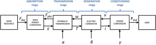
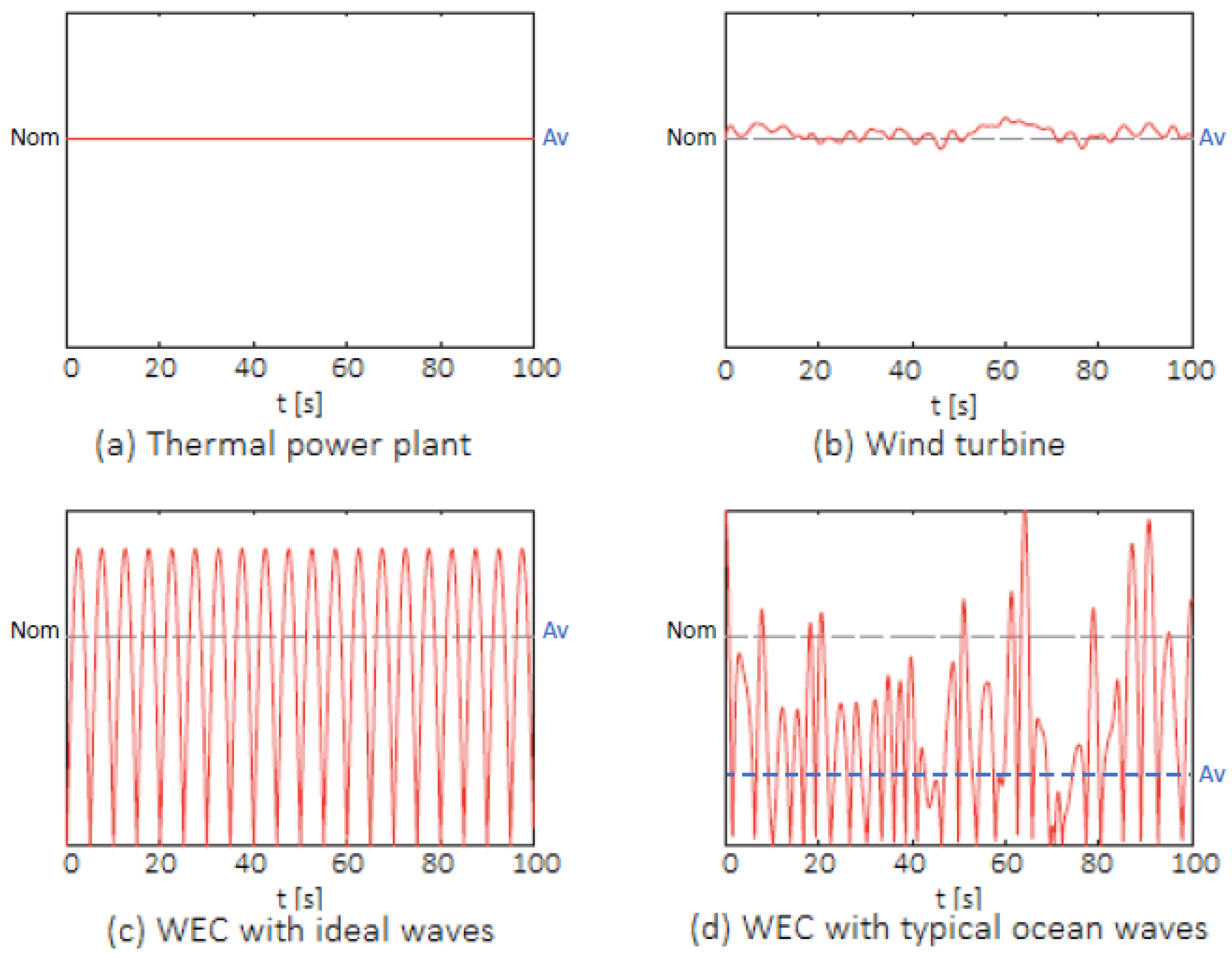
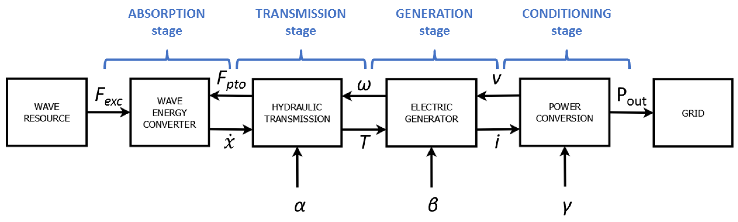
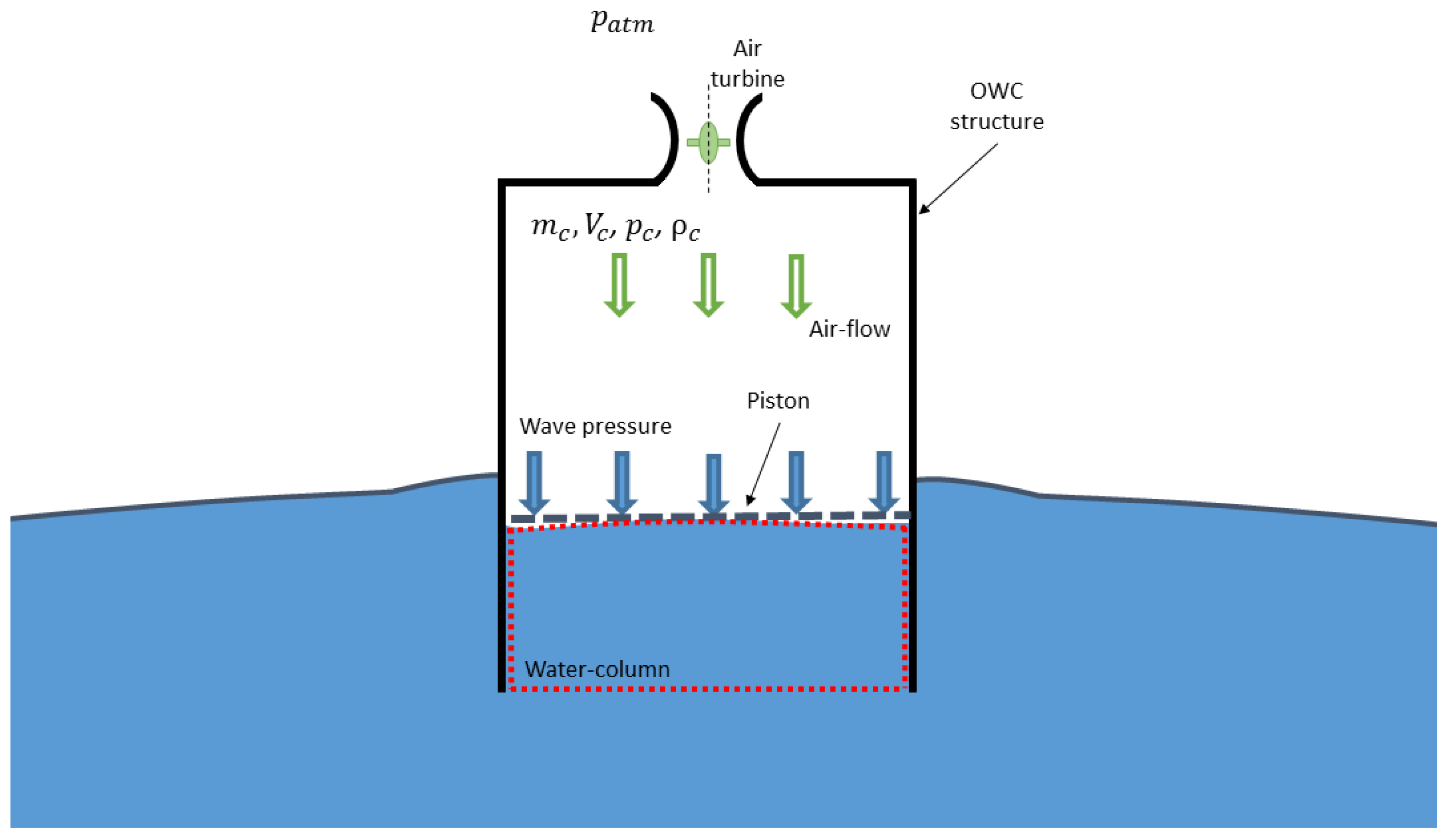
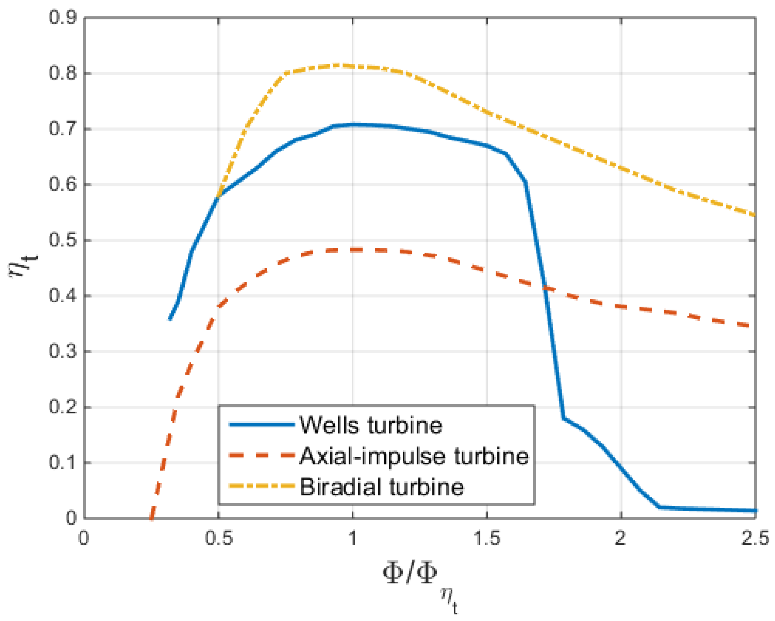
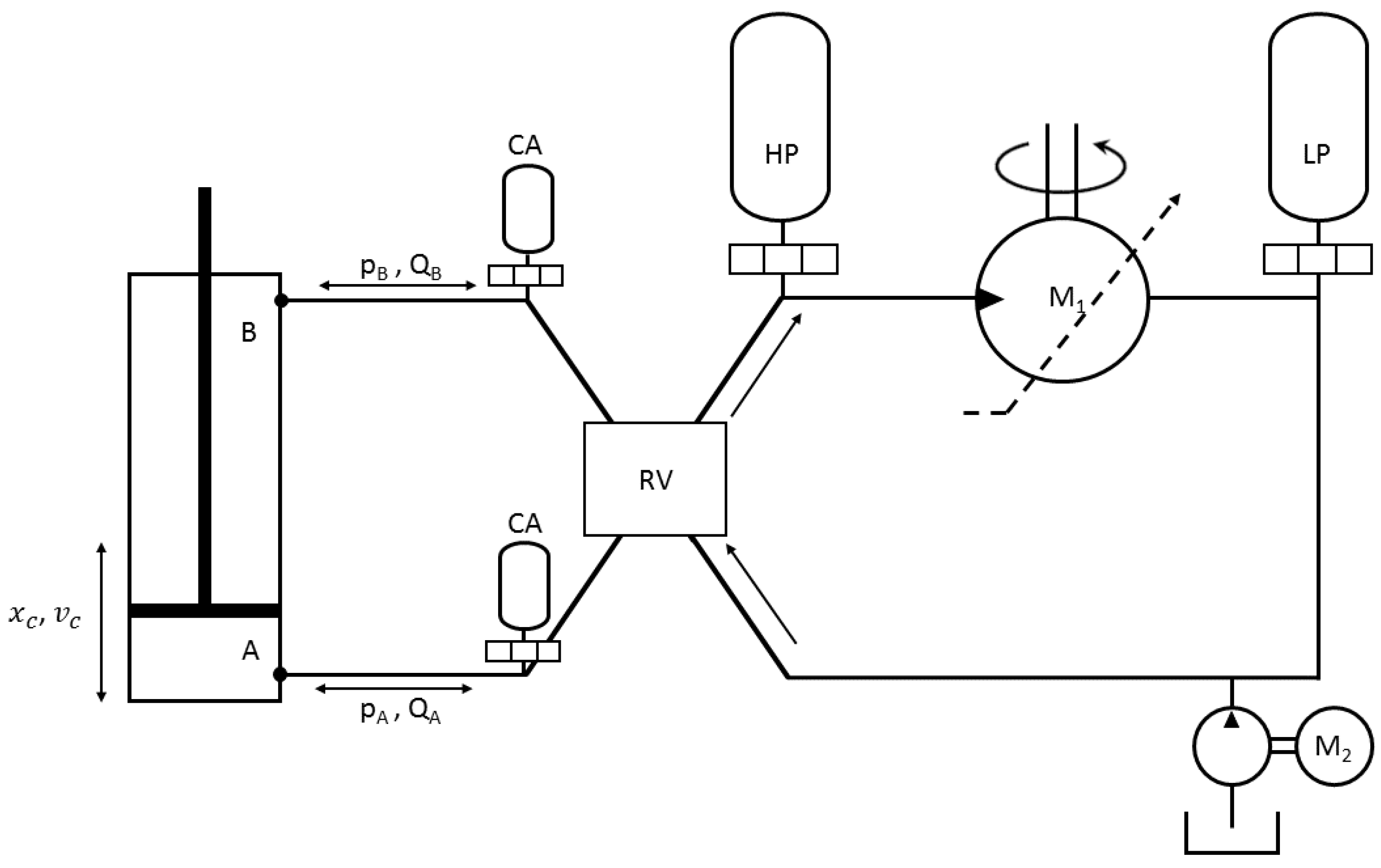
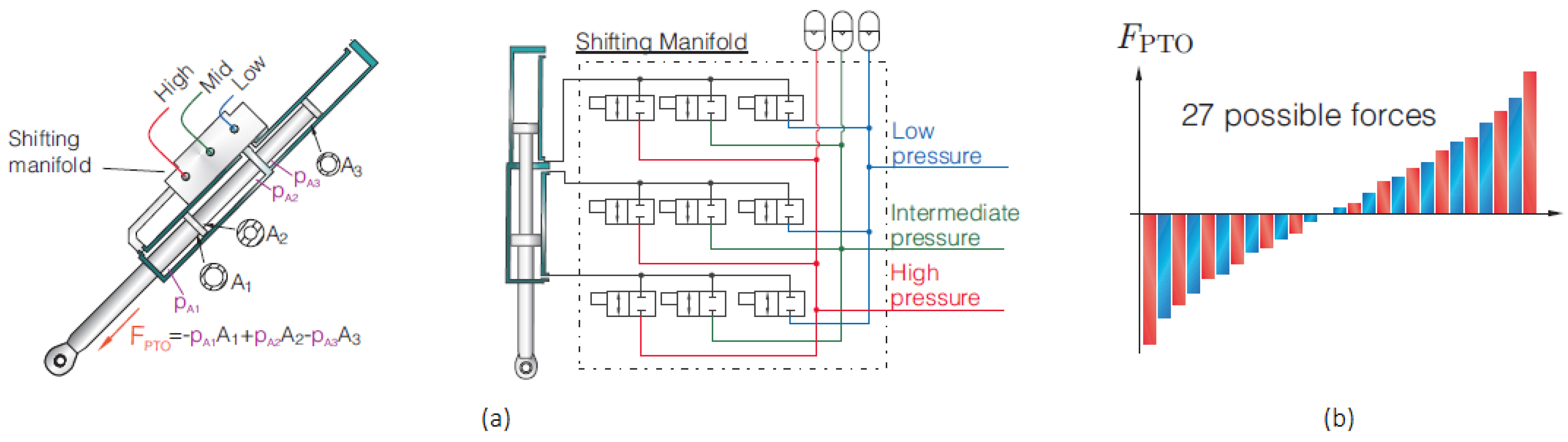
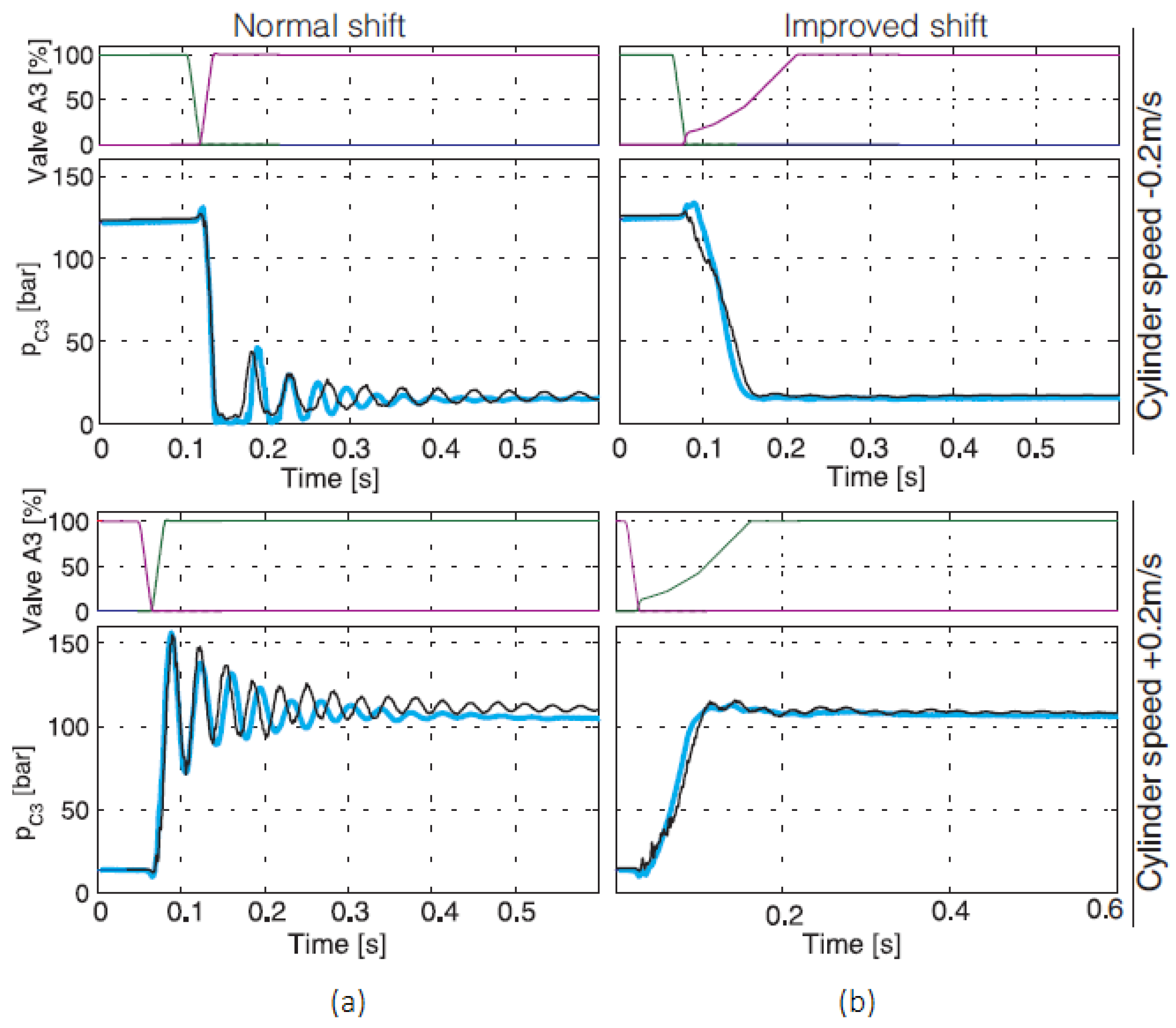
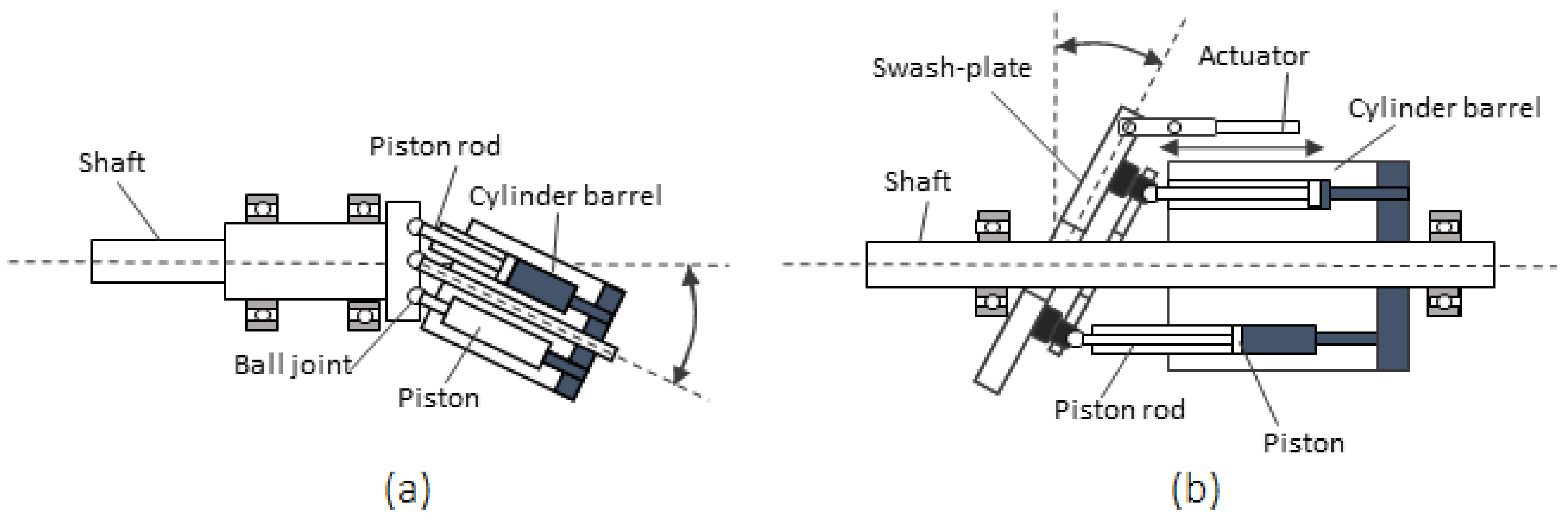
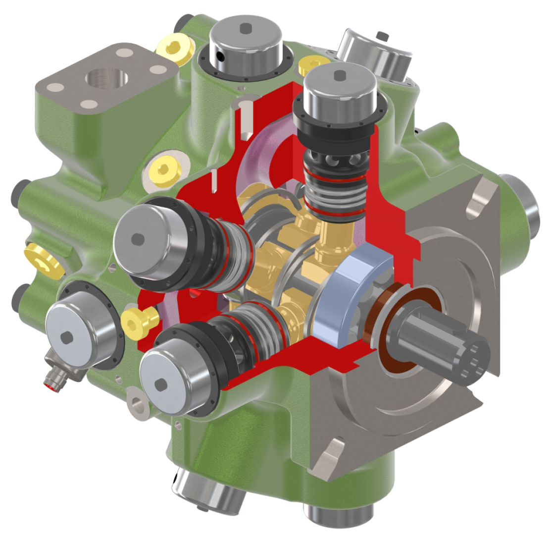
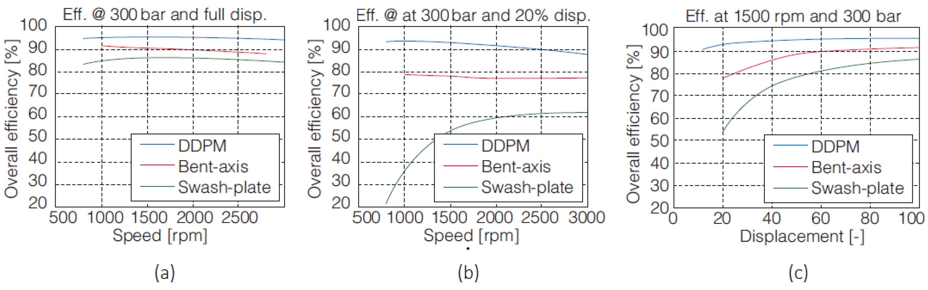
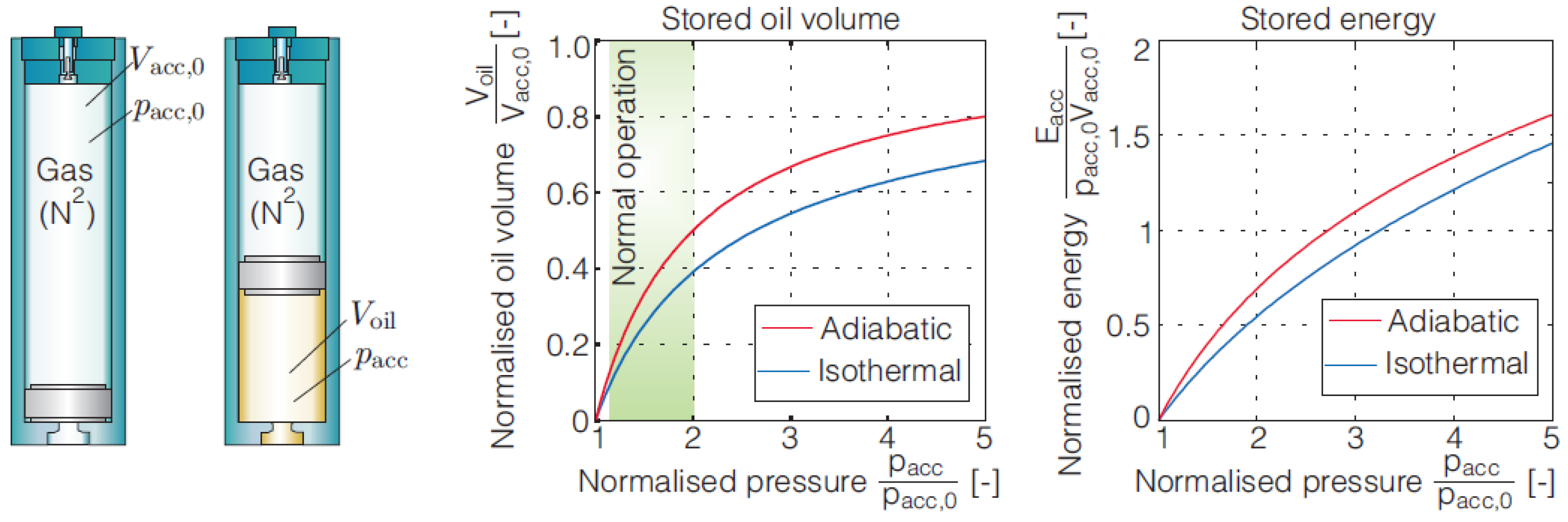
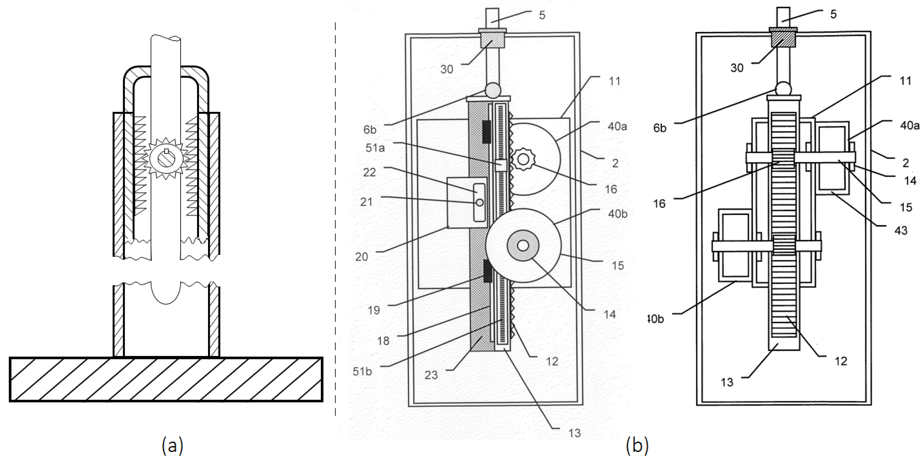
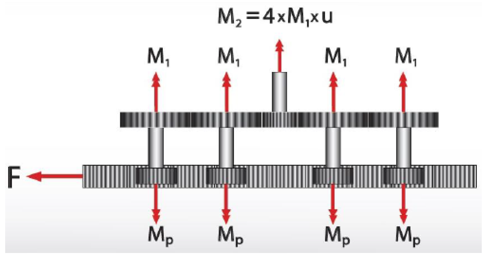
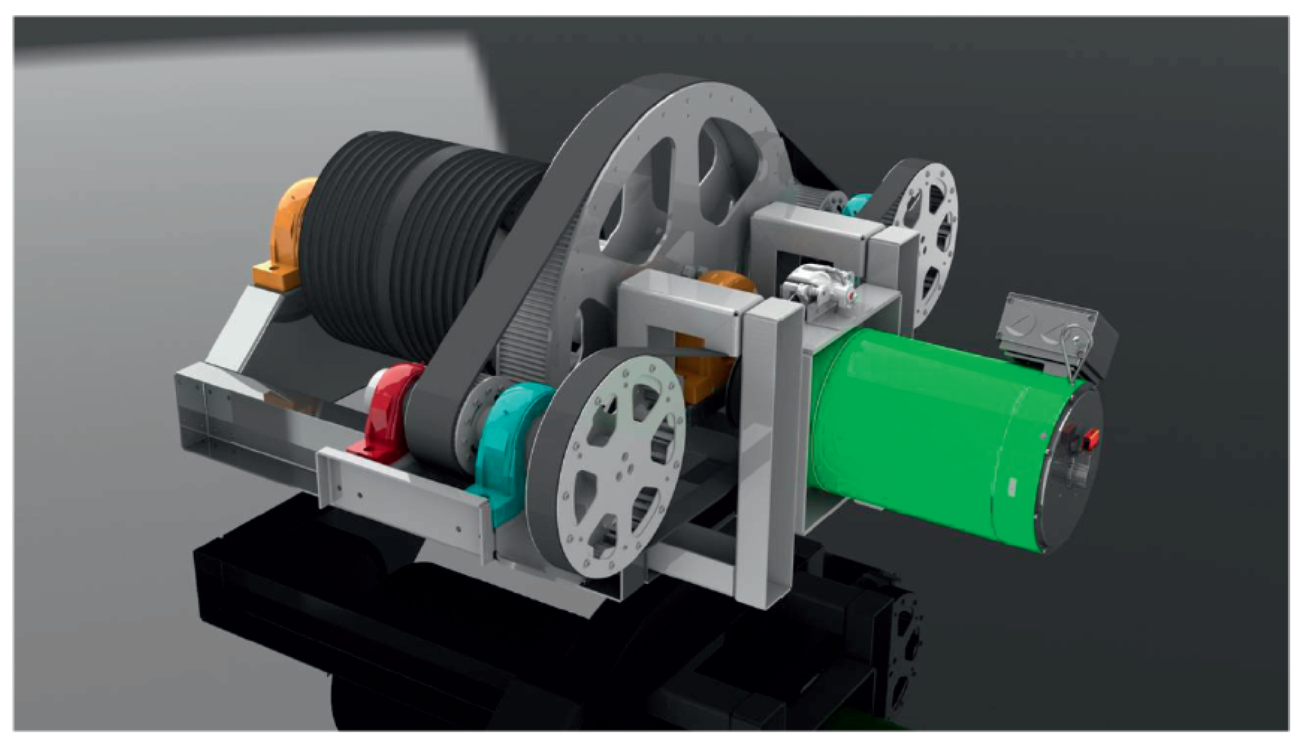
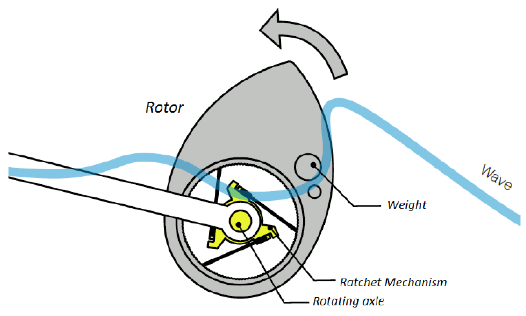
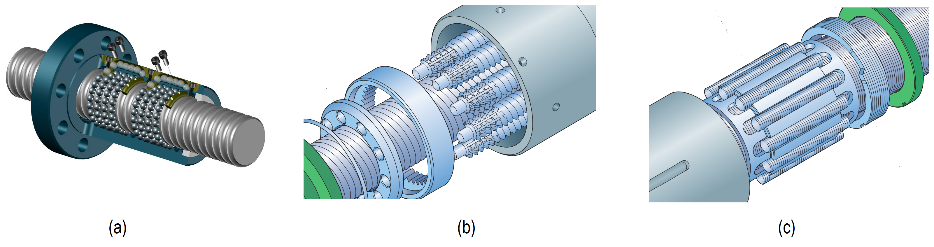
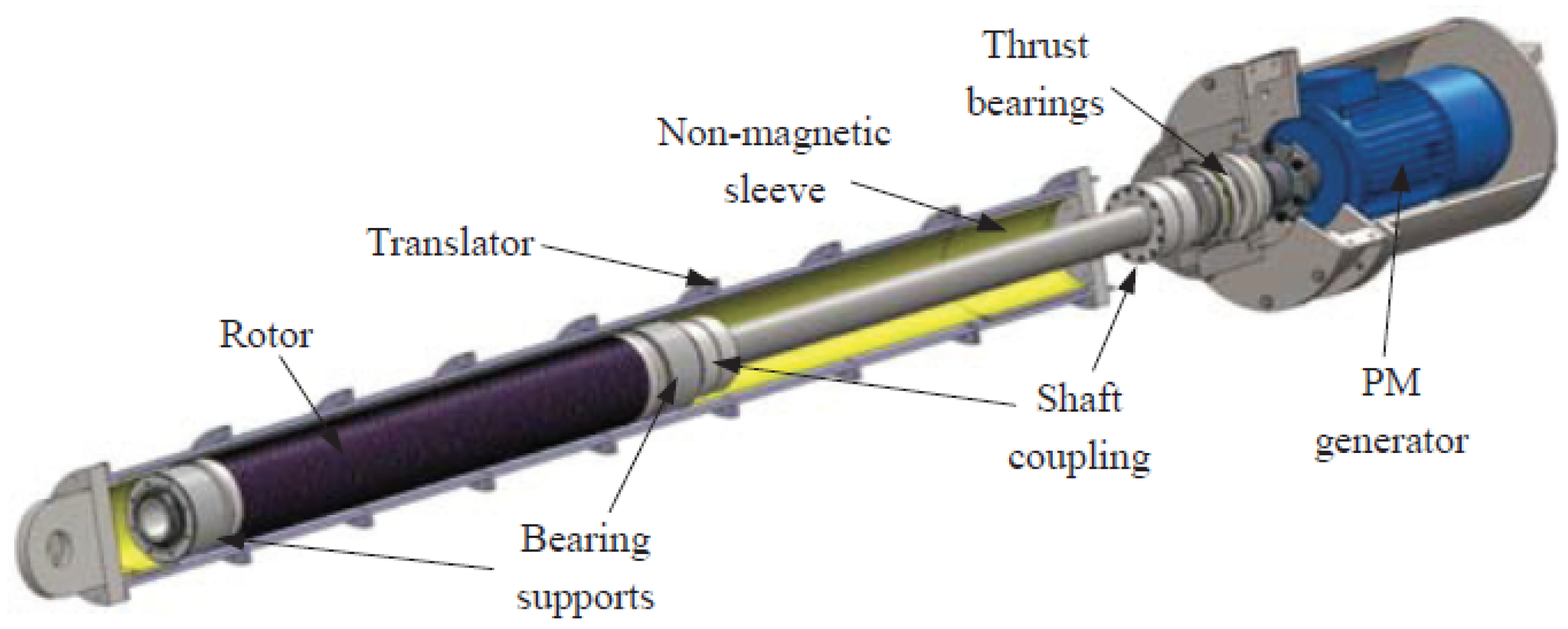
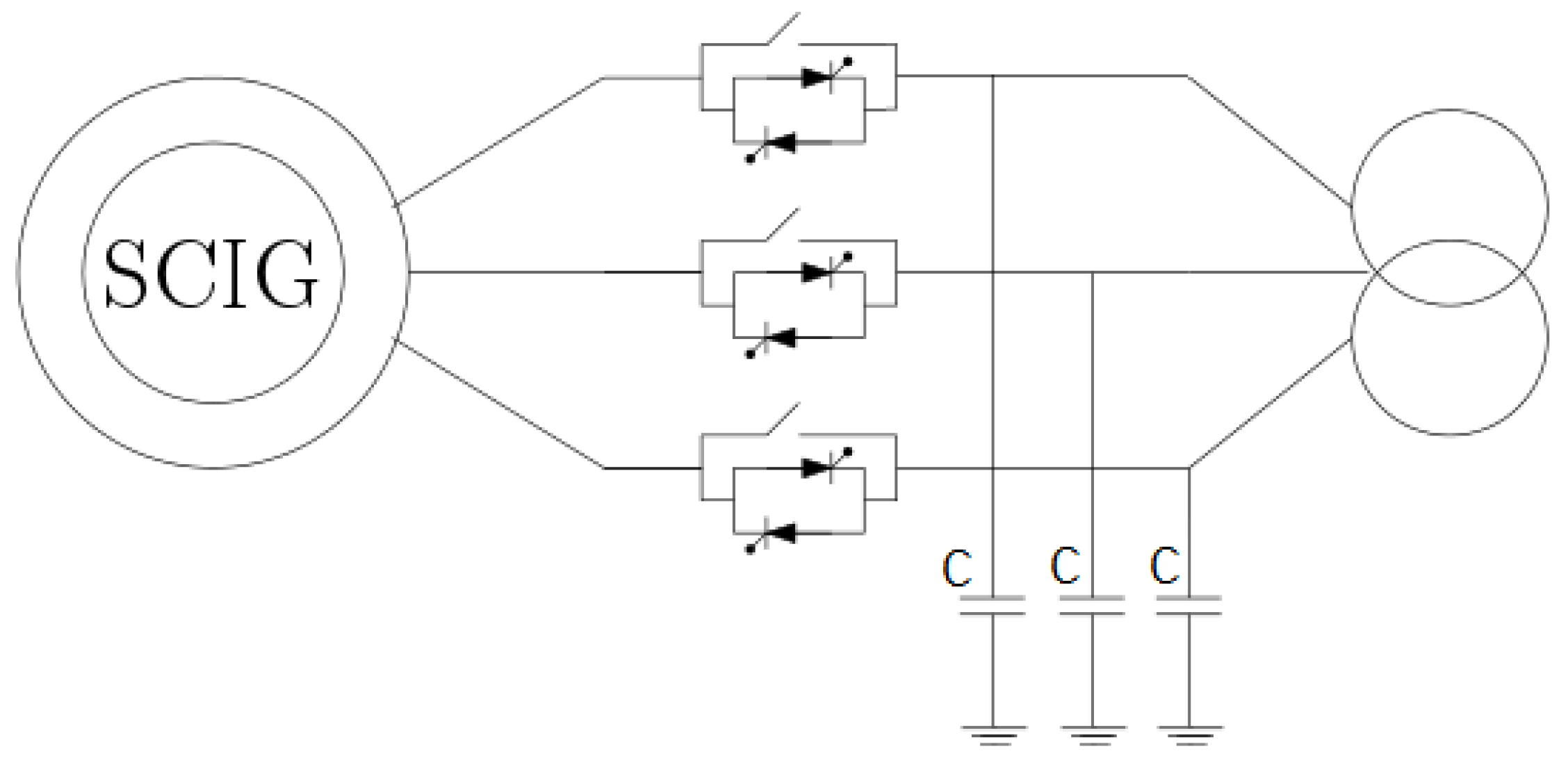
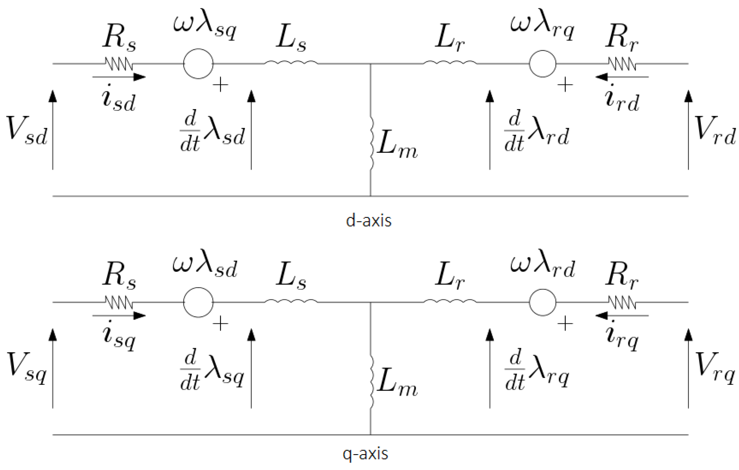
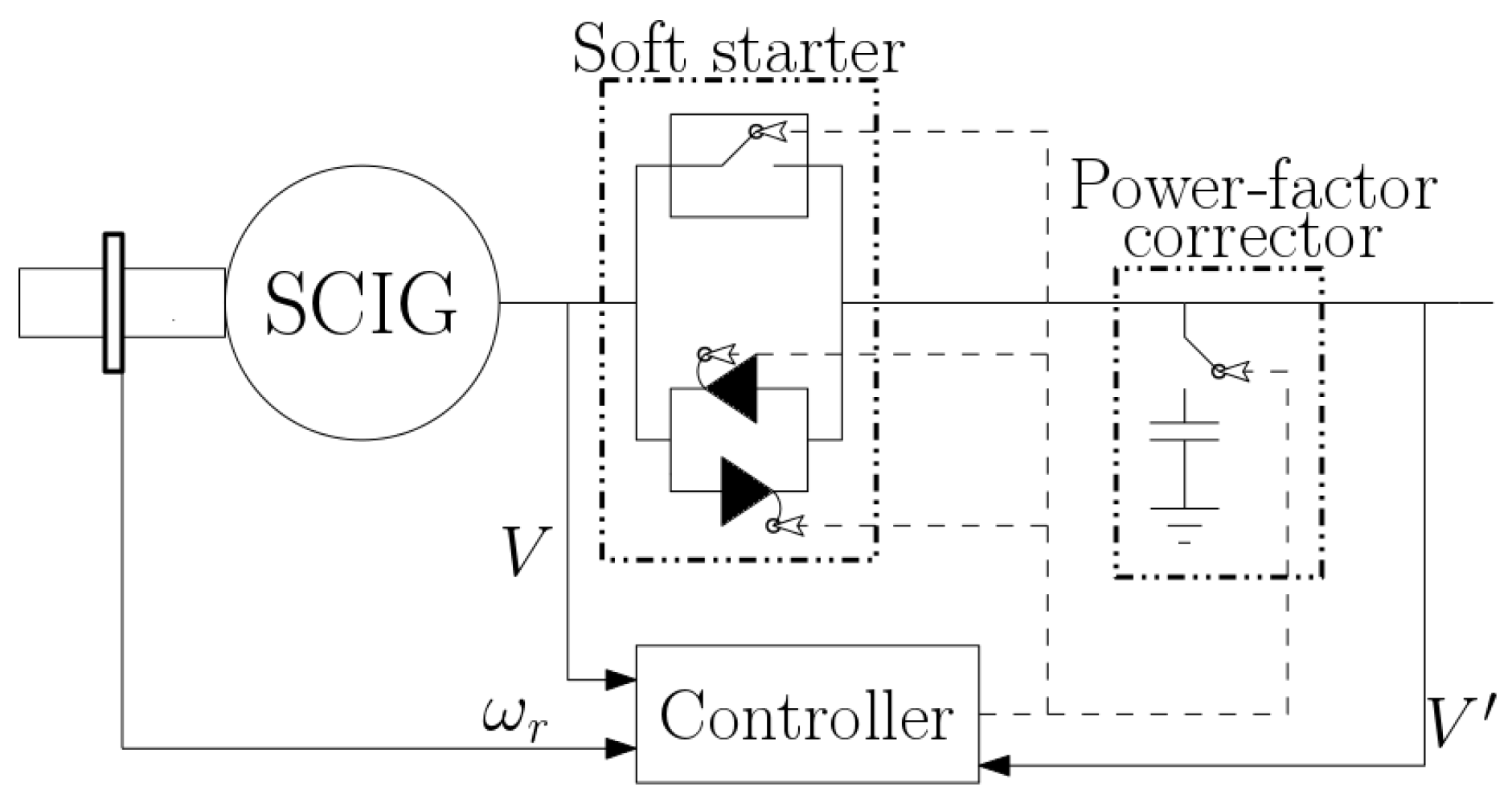
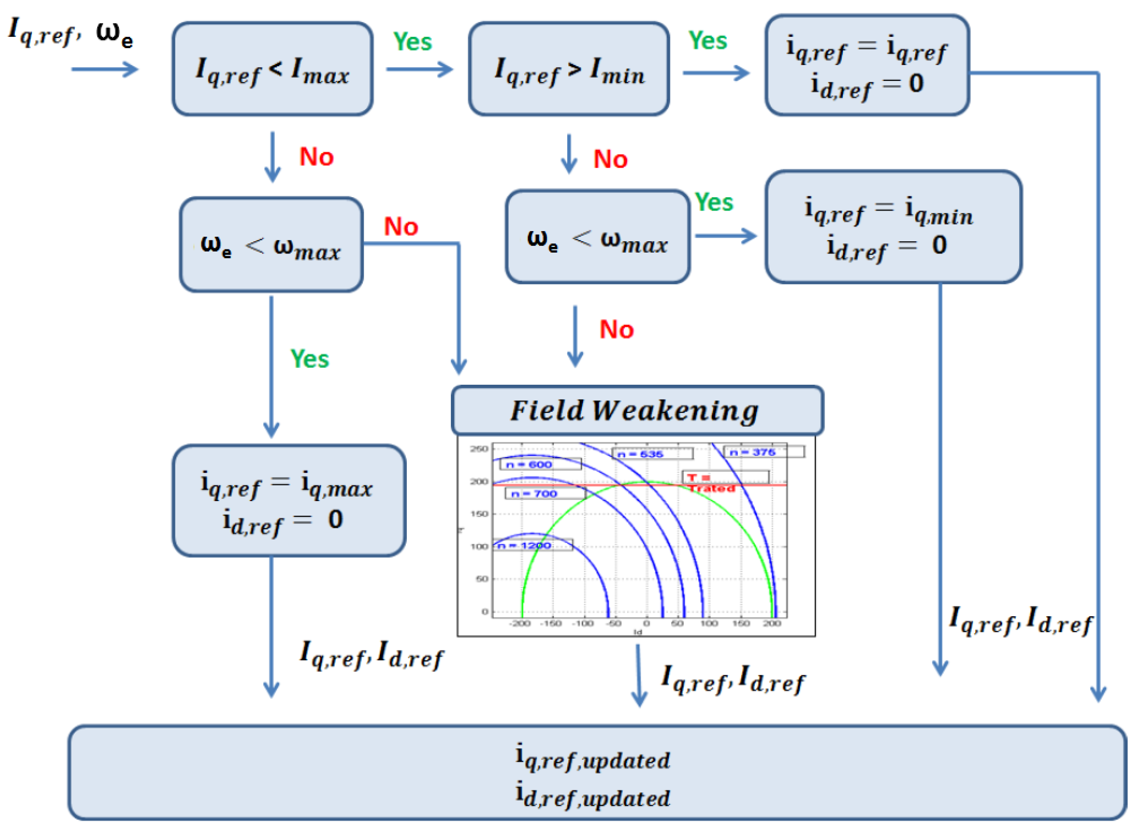
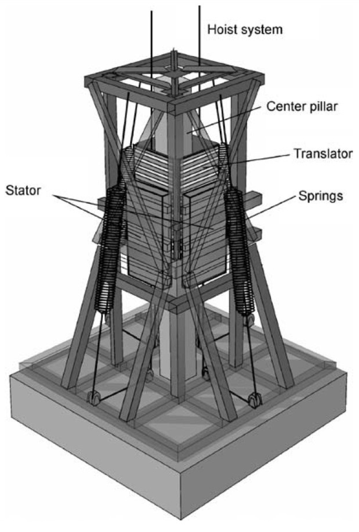
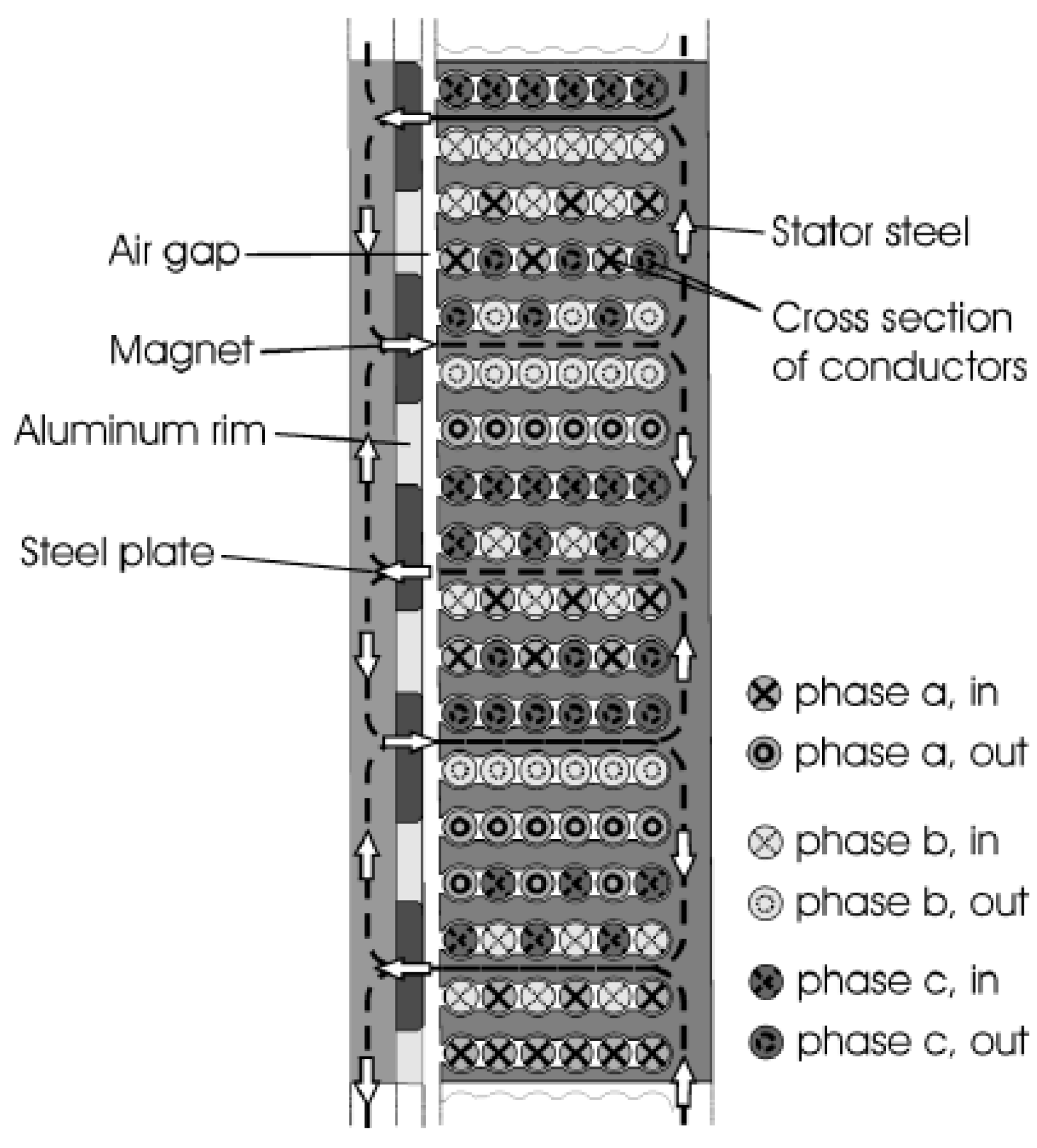
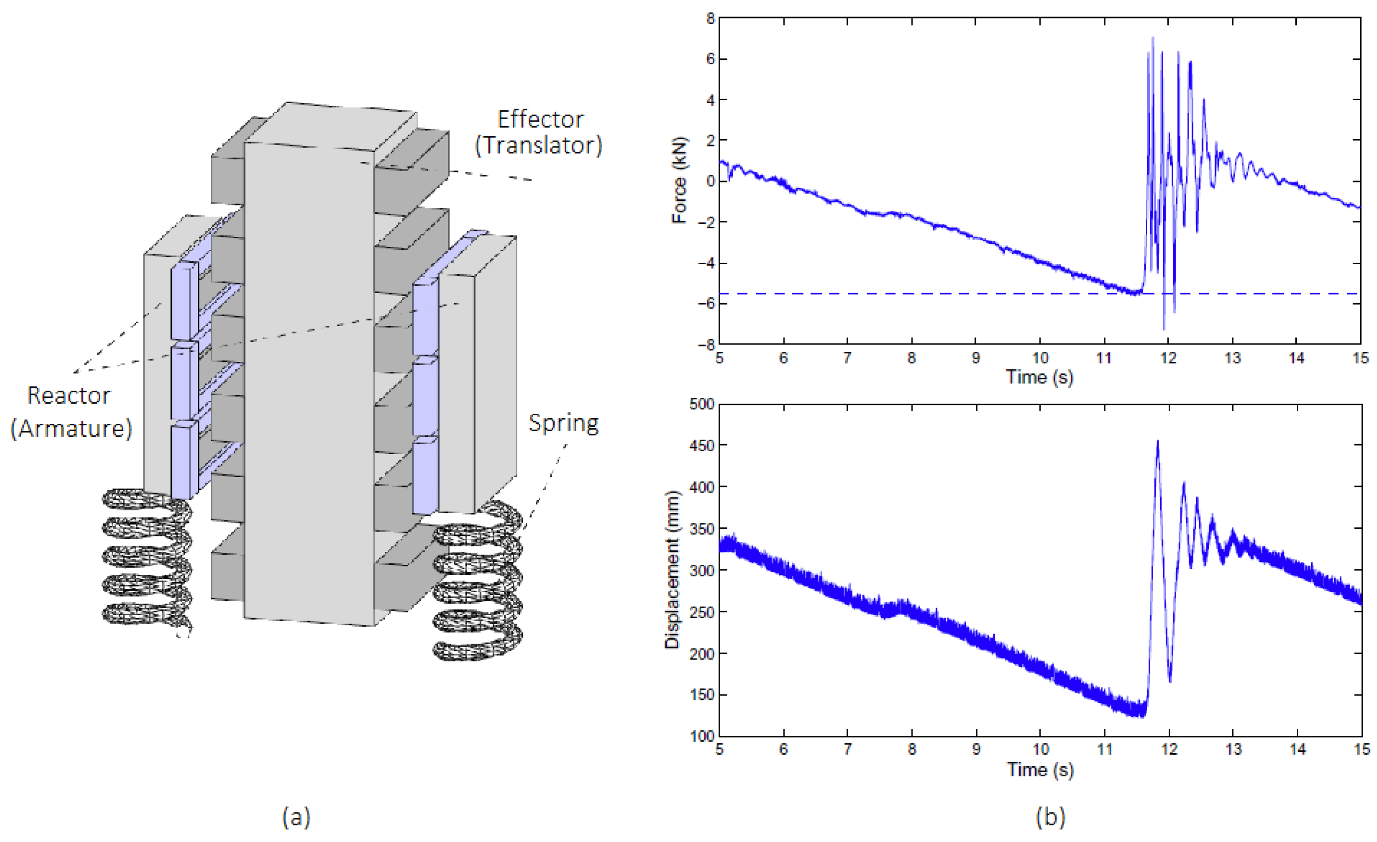
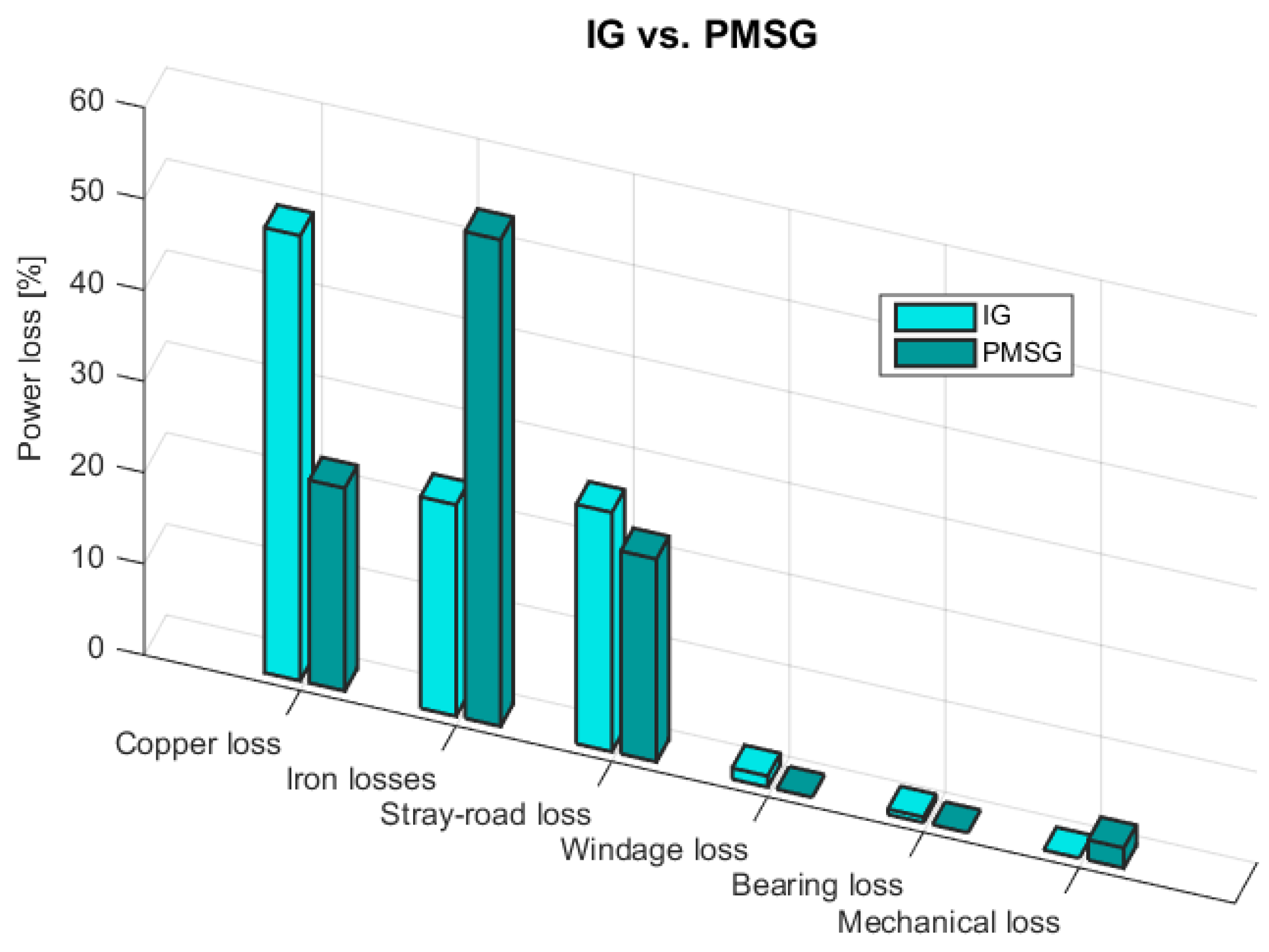
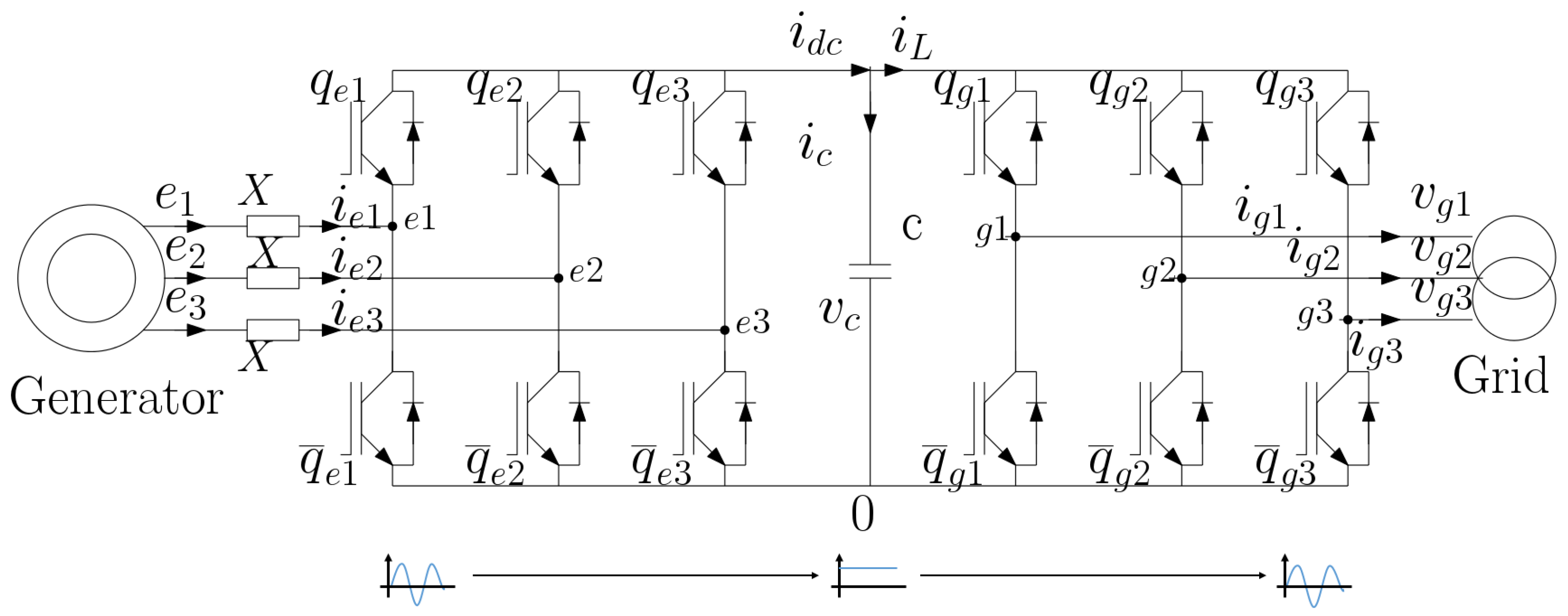
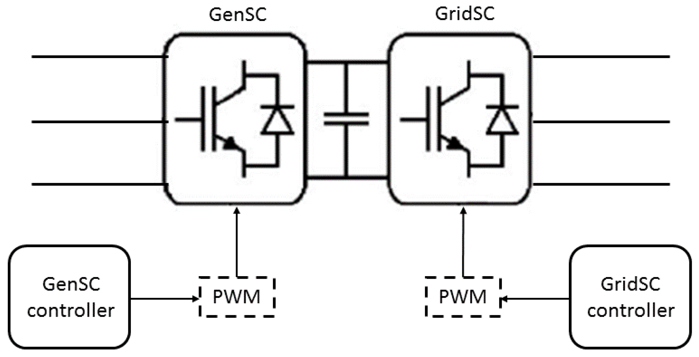
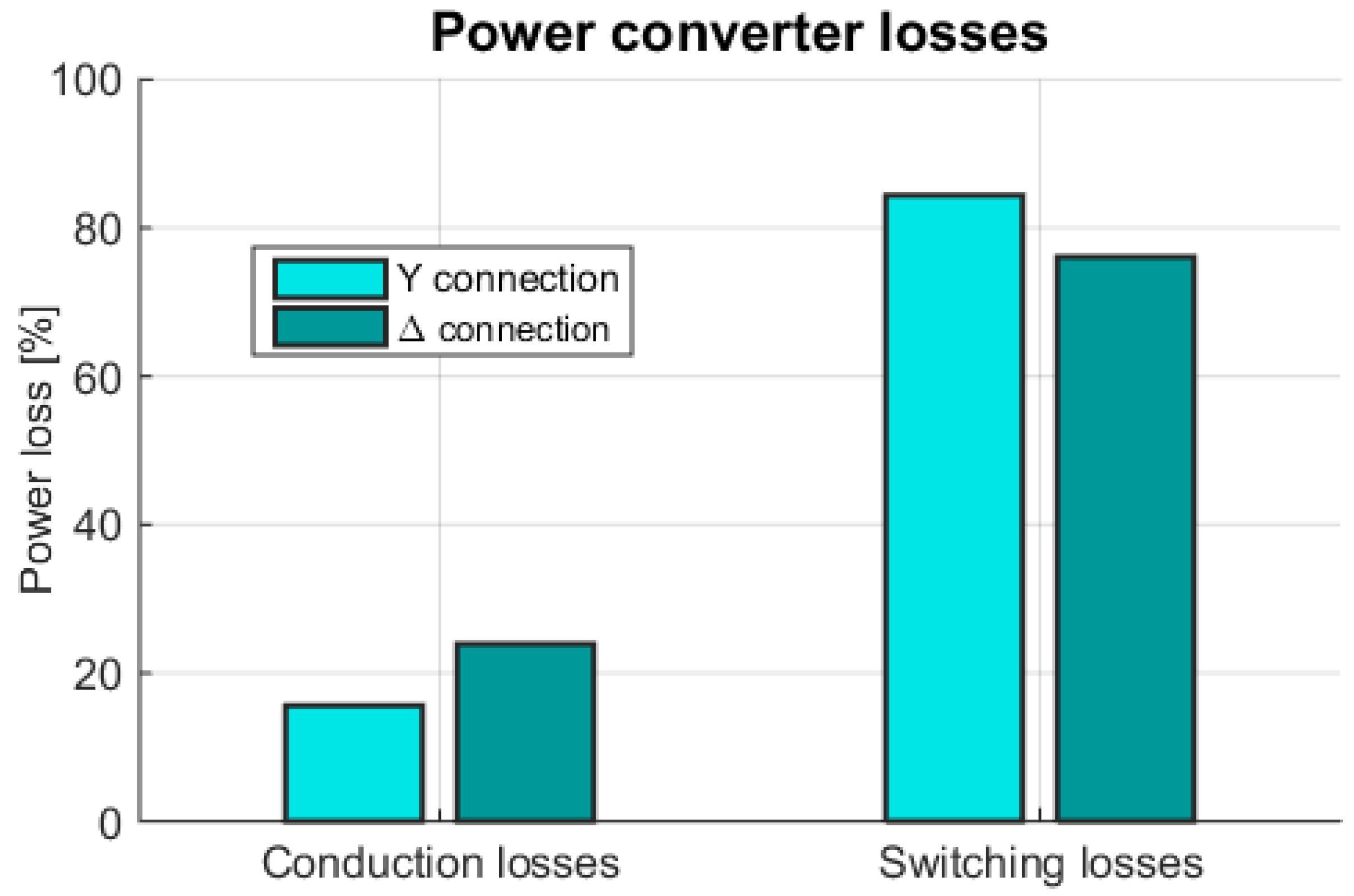
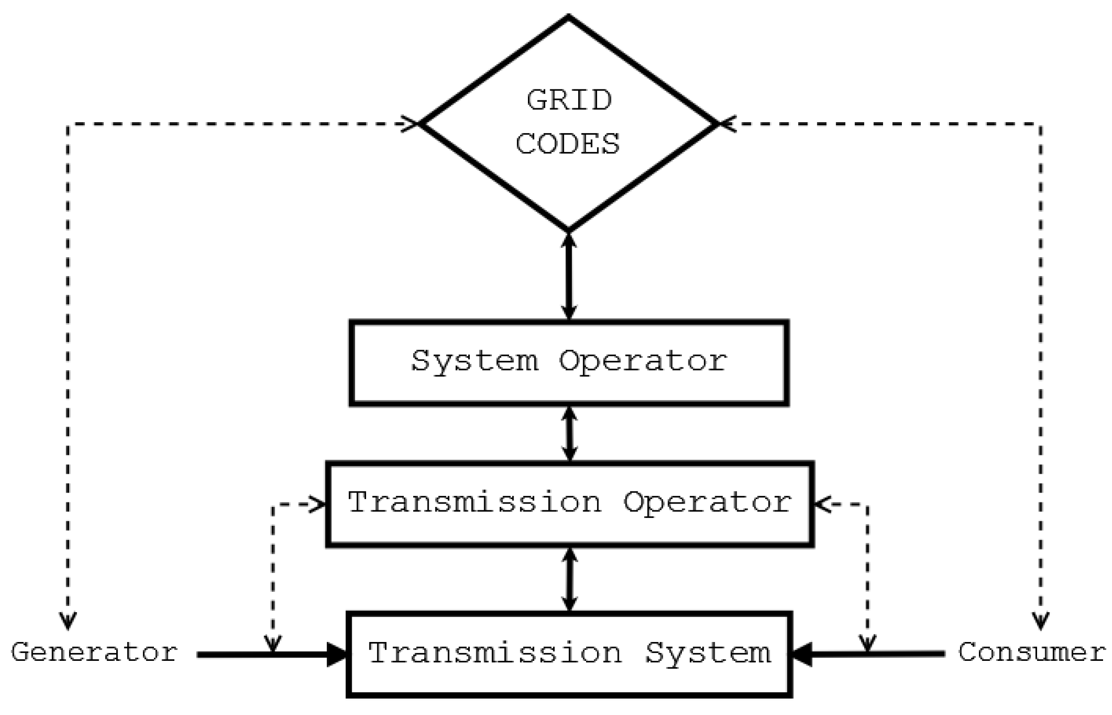
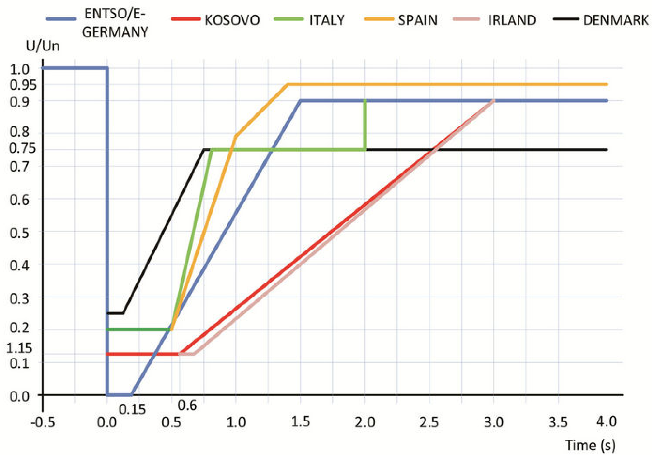
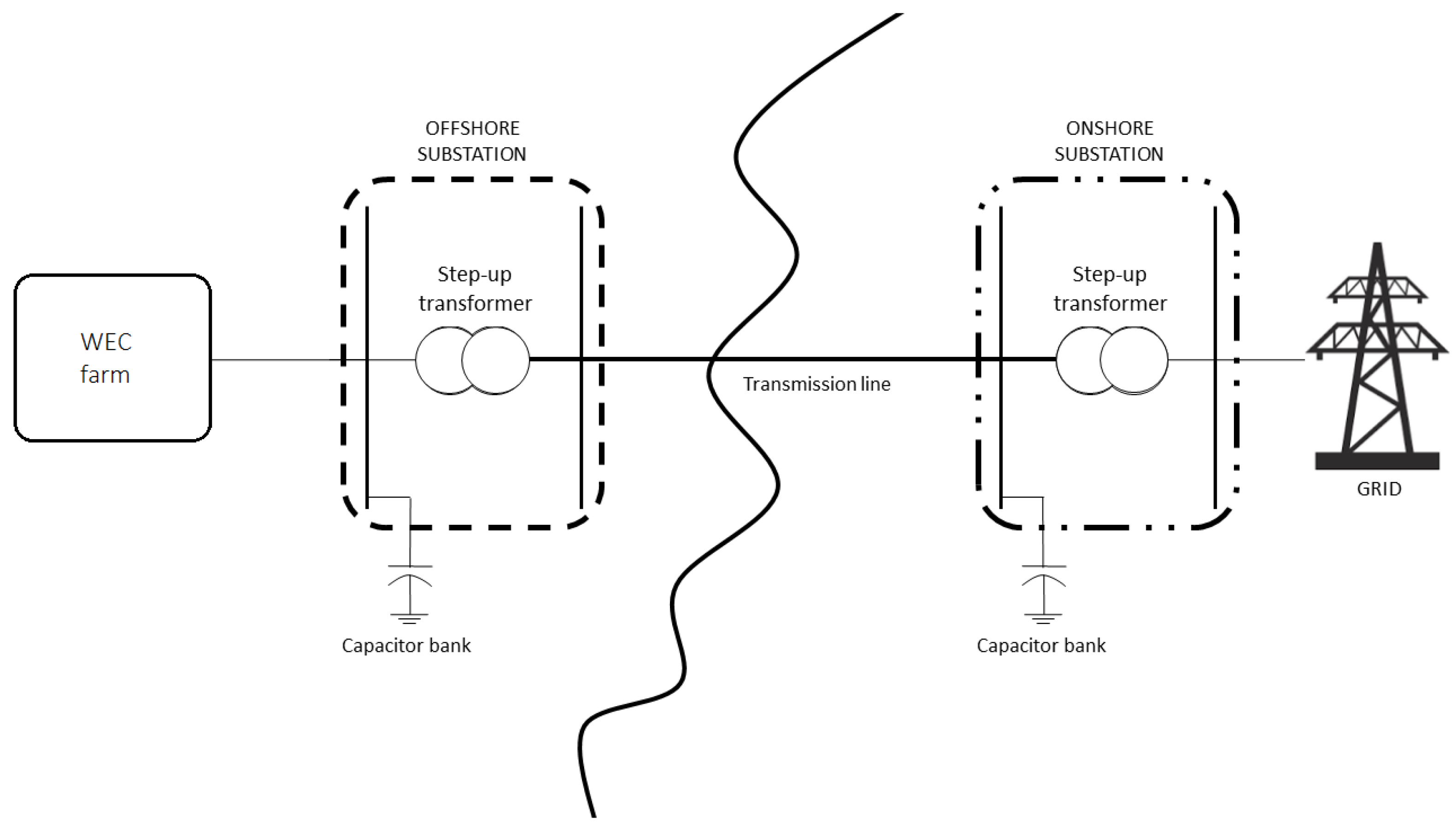
Table 1.
Literature review summary table, showing essential control characteristics for wave-to-wire (W2W) models. The following abbreviations are used in the table above: N/A for not applicable, cte. for constant, T for torque and η for efficiency.
| References | Hydrodynamic Model | Hydraulic Transmission | Electric Conversion | Grid Requirements | ||||||
|---|---|---|---|---|---|---|---|---|---|---|
| Cylinder | Valves | Accumulators | Motor | Electric Generator | Converter | |||||
| Fully Linear (Cummins) | Nonlinear Effects | Constraints | Losses | Losses | ||||||
| [8] | √ | × | Compressibility | × | adiabatic | × | × | × | ||
| [9] | √ | × | × | × | adiabatic | × | cte. T & | × | × | |
| [10] | √ | × | × | × | isothermal | cte. Pow. loss | dynamic | N/A | √ | |
| [11] | Viscous drag | × | × | × | adiabatic | √ | cte. T & | × | × | |
| [12] | NL restoring | × | × | × | √ | × | dynamic | N/A | √ | |
| [13] | √ | √ | √ | √ | √ | √ | Steady-state dynamics (NO transient) | map | × | |
| N/A | × | |||||||||
| [14] | √ | N/A | √ | √ | × | |||||
| [1] | √ | N/A | √ | √ | √ | |||||
| [15] | √ | N/A | dynamic | √ | ||||||
| [16] | √ | N/A | dynamic | × | ||||||
| Nominal Voltage | Normal Operating Ranges | |
|---|---|---|
| UK | Ireland | |
| 400 kV | 400 kV | 350–420 kV |
| 275 kV | 275 kV | 200–245 kV |
| 132 kV | 132 kV | 99–123 kV |
| Country | Frequency Range | Requirements |
|---|---|---|
| UK | 51.5–52 Hz | At least a period of 15 min of operation |
| 51–51.5 Hz | At least a period of 90 min of operation | |
| 49–51 Hz | Continuous operation | |
| 47.5–49 Hz | At least a period of 90 min of operation | |
| 47–47.5 Hz | At least a period of 20 s of operation | |
| Ireland | 49.5–50.5 Hz | Continuous operation |
| 47.5–52 Hz | Remain connected for a period of 60 min. | |
| 47–47.5 Hz | Remain connected for a period of 20 s | |
| above 50.2 Hz | No extra wind turbine shall be connected |
© 2016 by the authors; licensee MDPI, Basel, Switzerland. This article is an open access article distributed under the terms and conditions of the Creative Commons Attribution (CC-BY) license (http://creativecommons.org/licenses/by/4.0/).
Share and Cite
MDPI and ACS Style
Penalba, M.; Ringwood, J.V. A Review of Wave-to-Wire Models for Wave Energy Converters. Energies 2016, 9, 506. https://doi.org/10.3390/en9070506
AMA Style
Penalba M, Ringwood JV. A Review of Wave-to-Wire Models for Wave Energy Converters. Energies. 2016; 9(7):506. https://doi.org/10.3390/en9070506
Chicago/Turabian StylePenalba, Markel, and John V. Ringwood. 2016. "A Review of Wave-to-Wire Models for Wave Energy Converters" Energies 9, no. 7: 506. https://doi.org/10.3390/en9070506
Note that from the first issue of 2016, this journal uses article numbers instead of page numbers. See further details here.