
Cavitation Inception in Crossflow Hydro Turbines


1
Department of Mechanical and Manufacturing Engineering, University of Calgary, 2500 University Dr NW, Calgary, AB T2N 1N4, Canada
2
Faculty of Mechanical Engineering, Federal University of Pará –Av. Augusto Correa, N 1–Belém, PA 66075-900, Brazil
*
Author to whom correspondence should be addressed.
†
Current Address: Department of Mechanical and Manufacturing Engineering, University of Calgary, 2500 University Dr NW, Calgary, AB T2N 1N4, Canada
Energies 2016, 9(4), 237; https://doi.org/10.3390/en9040237
Submission received: 19 February 2016
/
Revised: 17 March 2016
/
Accepted: 21 March 2016
/
Published: 24 March 2016
(This article belongs to the Special Issue Hydropower)
Abstract
:Cavitation is a common flow phenomena in most hydraulic turbines and has the potential to cause vibration, blade surface damage and performance loss. Despite the fact that crossflow turbines have been used in small-scale hydropower systems for a long time, cavitation has not been studied in these turbines. In this paper, we present the findings of a computational study on cavitation inception in crossflow turbines. Cavitation inception was assessed using three-dimensional (3D) Reynolds-Averaged Navier–Stokes (RANS) computations. A homogeneous, free-surface two-phase flow model was used. Pressure distributions on the blades were examined for different flow rates, heads and impeller speeds to assess cavitation inception. The results showed that cavitation occurs in the second stage of the turbine and was observed on the suction side near the inner edge of the blades. For the particular turbine studied, cavitation always occurred at shaft speeds greater than that, giving the maximum efficiency for each combination of flow rate and head. The implication is that the useful operating range of crossflow turbines is up to and including the maximum efficiency point.
1. Introduction
This paper reports the results of a computational study on cavitation in crossflow turbines using three-dimensional (3D) Reynolds Averaged Navier–Stokes (RANS) simulations. Crossflow turbines are the most commonly used turbines in low-to-medium head small-scale systems, usually in the range of 5–300 kW. These turbines have a number of desirable characteristics, such as simplicity of design and low cost to manufacture, sturdy construction and a relatively flat and good efficiency curve over a wide range of operating parameters. In a crossflow turbine, curved circular blades are arranged radially around the axis of rotation and the ends of the blades are fixed to circular disks at the two ends (Figure 1). Unlike complex design shapes, such as in Pelton and Francis turbines, the most prominent feature of this design is the use of circular section blades, which can be easily designed and manufactured out of thin steel sheets using simple machines at low cost. The crossflow turbine is considered as a radial type impulse turbine, which operates in atmospheric conditions [1]. The flow passes radially through the impeller blades twice (Figure 1), hence the turbine is commonly known as crossflow turbine. As a consequence, power is extracted in two stages. Unlike other hydraulic turbines, the flow in a crossflow turbine is either a two-phase mixture of water and air or a three-phase mixture of water, water-vapor and air (if cavitation is present). The impeller is partially covered by water, and the rest of the flow domain is filled up by air and is characterized by free-surface effects. This results in a highly complex flow, in terms of physical understanding as well as numerical modelling and computations.
One of the important flow phenomena influencing the internal flow and performance loss in hydraulic turbines is cavitation. Cavitation occurs when the local fluid pressure falls below the vapor pressure of water and has the potential to cause vibration, damage to the blade surface and performance loss [2,3]. As a consequence, one of the major requirements in the design and operation of hydraulic turbines is to avoid cavitation. To the authors’ knowledge, no previous studies on cavitation in crossflow turbines have been reported in the literature. Most of the previous studies [4,5,6,7,8,9,10] on crossflow turbines are primarily focused on performance measurements, in attempts to improve the turbine efficiency. Recent computational studies [11,12,13] employing 3D steady state RANS simulations are mainly focused on validation studies for predicting the turbine performance. It is interesting to note that crossflow turbines are mainly used in small-scale systems in remote locations around the world, where the cost and simplicity of design and manufacturing are the critical considerations. As a consequence, the detailed performance characteristics, primarily the maximum efficiency and cavitation, have not been the critical considerations until recently. As high-performing turbines are important for the overall sustainability of such systems, these two design aspects must be addressed in future designs. This paper concentrates on the second issue: cavitation. Experimental observations and measurements of cavitation in turbines involve complexity as well as high cost. Therefore, computational studies employing the solutions of the Navier–Stokes equations of various fidelity (because of their ability to determine pressure everywhere in the flow) are needed to gain fundamental understanding of the underlying flow features and the possibility of cavitation. It is extremely important to characterize cavitation, if present, in order to avoid or minimize it and improve the overall turbine performance. The ability to avoid or minimize cavitation could lead to better turbine designs and longer lifetimes of installed turbines.
The rest of the paper describes the main findings of this study and is organized as follows. Section 2 provides a brief overview of the methods to determine the onset of cavitation and Section 3 describes the computational methodology used in the study. Section 4 presents the summary of validation study and important results and discussion on cavitation at different operating conditions. The emphasis is on the conditions under which cavitation begins, rather than its full development, on the grounds that mapping the boundary between cavitating and non-cavitating flow is the most important design requirement. Section 5 summarizes the key conclusions drawn from this study.
2. Cavitation
Cavitation is a common phenomena in most hydraulic turbines, such as Francis, Kaplan, Propeller, and Pelton, which can potentially lead to performance loss and damage to the blade surfaces [3] Cavitation is a two-phase (water and water-vapor) interaction that involves vaporization of water and condensation of water-vapor. Vapor bubbles are formed when the local pressure in the flow field falls below the vapor pressure of water (e.g., 3.17 kPa at ) [2]. Cavitation primarily occurs in separated, accelerated and recirculating flow regions near curved surfaces [3], such as in the impeller of the crossflow turbine. Local flow acceleration and the recirculating fluid elements (in vortex regions) cause a decrease in local pressure. For a given turbine geometry, the variables that contribute to these effects are the flow rate (Q), head (H) and the impeller speed (N). The dimensionless parameter used to characterize cavitation is the cavitation number (σ), which is defined as [14]:
where ) and are respectively the reference and saturated water-vapor pressures in the upstream flow (inlet of the impeller), is the atmospheric pressure, is the density of water and is the reference relative velocity in the upstream flow (inlet of the impeller). Equation (1) shows that cavitation is directly related to the ratio of drop in local pressure head and the dynamic head. Note that the dynamic head is closely related to the inertia of the local fluid motion, influenced by the impeller rotational speed N. In other words, the possibility of the local pressure being less than the vapor pressure is due to the effects of temporal or local variation of the velocity or the dynamic head [14,15]. For a given geometry and the flow conditions, the inception of cavitation () occurs when σ is equal to the minimum value of the coefficient of pressure () [14]. Here, the pressure coefficient is defined by:
where p and are respectively the local pressure on the blade surface and the relative velocity of water at the impeller inlet. So the condition for the inception of cavitation () is written as:
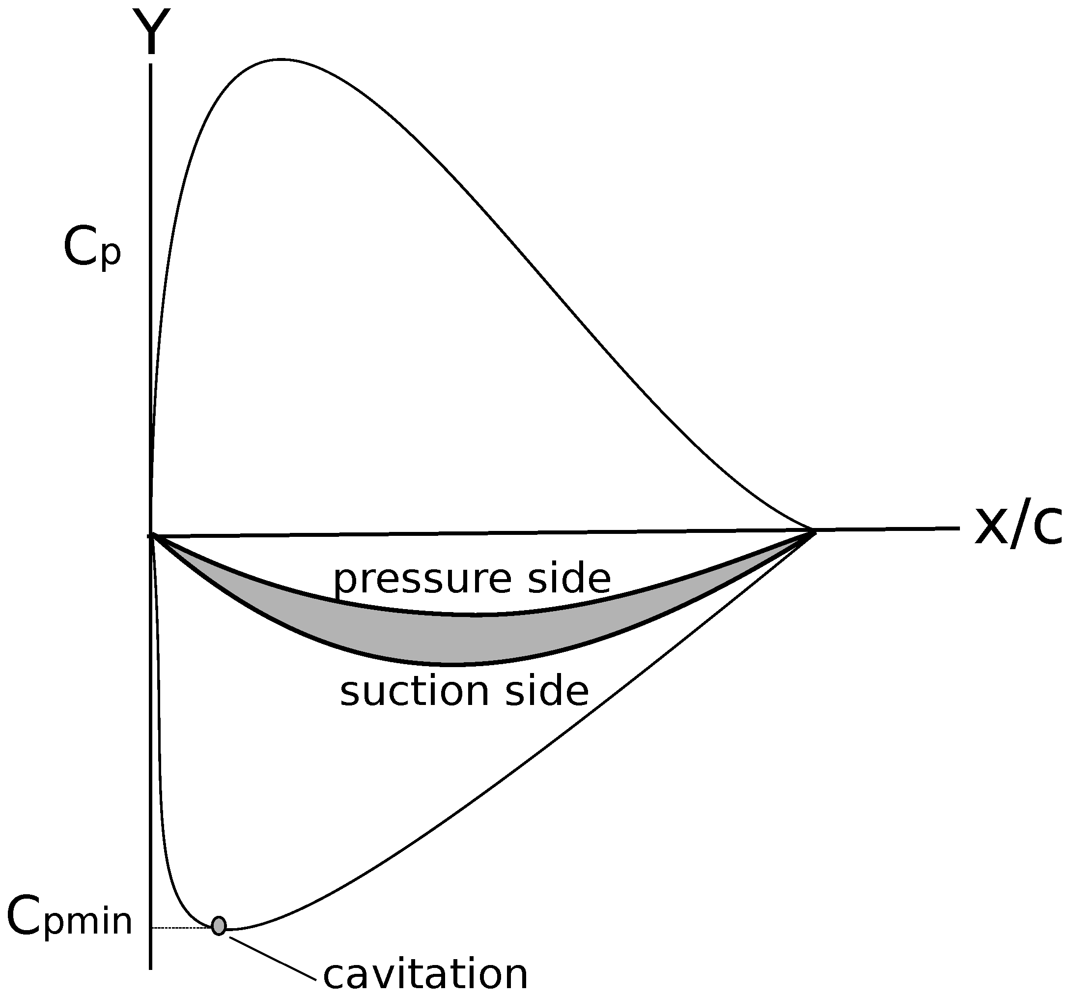
which is used widely for the determination of cavitation onset, e.g., [16]. It is noted from Equation (3) that further reduction of σ from increases cavitation. is an important parameter in the design as it is related to hydrodynamic loading of the blades and can be used as a criterion to minimize or avoid cavitation. depends on the blade geometry (or impeller geometry) and the Reynolds number. To minimize or avoid cavitation, on the blades can be increased by modifying the geometry of the blades and their stacking in the impeller. The distribution of on a cavitating blade in the impeller is schematically illustrated in Figure 2. The cavitation number σ can be reduced further by gradually reducing either the static pressure head or increasing the rotational speed of the impeller. As σ is reduced to , cavitation bubbles form on the low-pressure surfaces (usually starting at the leading edge) of the impeller blades and when they move into the higher-pressure regions, they collapse implosively. If the pressure in the neighbourhood of the cavity rises above the vapor pressure, the cavity collapses and it is heard as a loud noise in the turbine. In addition to performance deterioration, continuous collapse of cavities can rapidly erode the blade surfaces, produce vibration and eventually destroy them.
3. Computational Methodology
In this study, computational analysis is focused on investigating the key flow features that are related to the inception of cavitation in the impeller. As the aim of the study is to develop an understanding of the average flow field characteristics to determine the onset of cavitation, computations were carried out using 3D steady and unsteady RANS simulations with reference to a small-scale (7 kW) crossflow turbine. For solving the RANS equations, commercial computational fluid dynamics (CFD) code ANSYS CFX [17] was used. The RANS simulations have shown satisfactory results for predicting the performance for this class of turbomachinery problems [11,12,13]. The turbine configuration considered in this study is shown in Figure 1 and the corresponding geometrical parameters are presented in Table 1. The angle of attack (α) of the absolute velocity of the flow at the impeller inlet is 16 and the inlet and exit blade angles are 30 and 90 respectively. The impeller blades have a radius () of 52.14 mm. is the radius of the circular blade profile. This turbine was experimentally tested by Dakers and Martin [18], and all the geometrical parameters and performance data at different operating conditions (flow rate, head and impeller speed) needed for assessing the validity of the used computational model are available.
3.1. Multiphase and Turbulence Modelling
During normal operations without cavitation, the flow in a crossflow turbine is a two-phase mixture of water and air, which is characterized by free-surface effects. The impeller is only partially covered by water and the rest of the flow domain is filled by air. If cavitation is present, the flow would be a three-phase mixture of water, water-vapor and air. As a consequence, the flow in a crossflow turbine becomes highly complex in terms of physical understanding as well as numerical modeling; no generalized perfect numerical models are currently available to study such flows. However, lower-fidelity numerical models are available, which can capture the main flow features within an acceptable accuracy. In this study, the flow was modelled as a two-phase, homogeneous free-surface (water and air) flow as this is the computationally simplest multiphase flow model and has shown good performance for predicting the crossflow turbine performance. Using a two-phase model, inception of cavitation can be predicted based on the criteria of Equation (3). In a homogeneous multiphase flow, each fluid may possess its own flow field or all fluids may share a common flow field. The fluids are not mixed on a microscopic scale, rather they are mixed on a macroscopic scale with a discernible interface between them. With this model, the imposed kinematic and dynamic conditions are that water and air share the same pressure and velocity fields as well as the turbulence fields [2,16]. The free-surface model attempts to resolve the interface between the fluids by imposing these conditions [2,16]. For brevity, the continuity and momentum equations of the multiphase flow are omitted here; a more detailed discussions on multiphase model can be found in [14,16].
For the turbulence model, shear stress transport (SST) k-ω turbulence model was used because it has shown better performance in turbomachinery flows than other two-equation models. Flows in turbines inherently involve separation due to curvature and rotation. The SST k-ω turbulence model is a two-equation model for the turbulence kinetic energy (k) and the specific dissipation rate (ω) that consists of blending of k-ω and k-ω models based on proximity to the walls [19,20]. This model improves the k-ω model by using the blending function in the near-wall region, which activates the standard k-w model and transforms to the k-ε model away from the wall. This idea originates from Menter’s observation that the basic k-ω model overpredicts the level of shear stress in adverse pressure gradient boundary layers [19]. The k-ε model is found to perform poorly in adverse pressure gradients but better in free-shear layers [19]. Therefore, turbulent viscosity () is modified using a limiter function to account for the transport of turbulent shear stress, which shows better agreement to the experimental results in flows that involve adverse pressure gradients, streamline curvature and the onset of separation [19,20]. The predictive capability of this model for the onset and amount of separation at adverse pressure gradients has been found better than the standard k-ϵ or k-ω models [19]. For brevity, the transport equations for the SST k-ω turbulence model have been omitted and can be found in [17,20]. For solving the RANS equations, high-resolution upwind scheme with double precision was used in order to ensure convergence, accuracy and consistency in the computations [16].
3.2. Computational Domain and Boundary Conditions
For the 3D steady and unsteady RANS computations, an unstructured tetrahedral mesh with refined hexahedral elements in the near wall region was used. The mesh was refined near the wall () as the SST k-ω turbulence model performs better at this mesh resolution [16]. is a non-dimensional parameter, which defines the distance of the first mesh node from the wall. Since accuracy of computational results is one of the most important aspects in numerical simulations, a grid convergence study was carried out by gradually refining the mesh size starting from 2.1 million elements until an acceptable numerical accuracy was achieved for the turbine power output. A total of 5.4 million elements were required to produce a grid independent solution for the turbine power output, which corresponds to less than 0.1% numerical uncertainty in the computed results (summarized in Table 2). The numerical uncertainty was computed based on the relative error between the results of two consecutive mesh sizes. Moreover, a good agreement between the computed results and the experimental results was found, which further validates the suitability of the used mesh. The comparison of the experimental and CFD results are presented in the next section.
The computational domain is divided into two sub-domains: a stationary domain consisting of the nozzle and the casing and a rotating domain consisting of the impeller. General grid interface (GGI) was used for connecting the two sub-domains; GGI allows update on interface position at each time step while the relative positions of the grids on each side of the interface change. GGI also allows non matching grid points to communicate with each other via 3D interpolation process [16].
The imposed inlet and outlet boundary conditions correspond to the experimentally tested values for the heads H and flow rates Q at different impeller speeds N. At the inlet, total pressure corresponding to the operating head H was specified with the turbulence intensity of 5%. At the outlet, bulk mass flow rate () was specified. At the vents, opening type of boundary condition was specified.
4. Results and Discussion
4.1. Numerical Validation
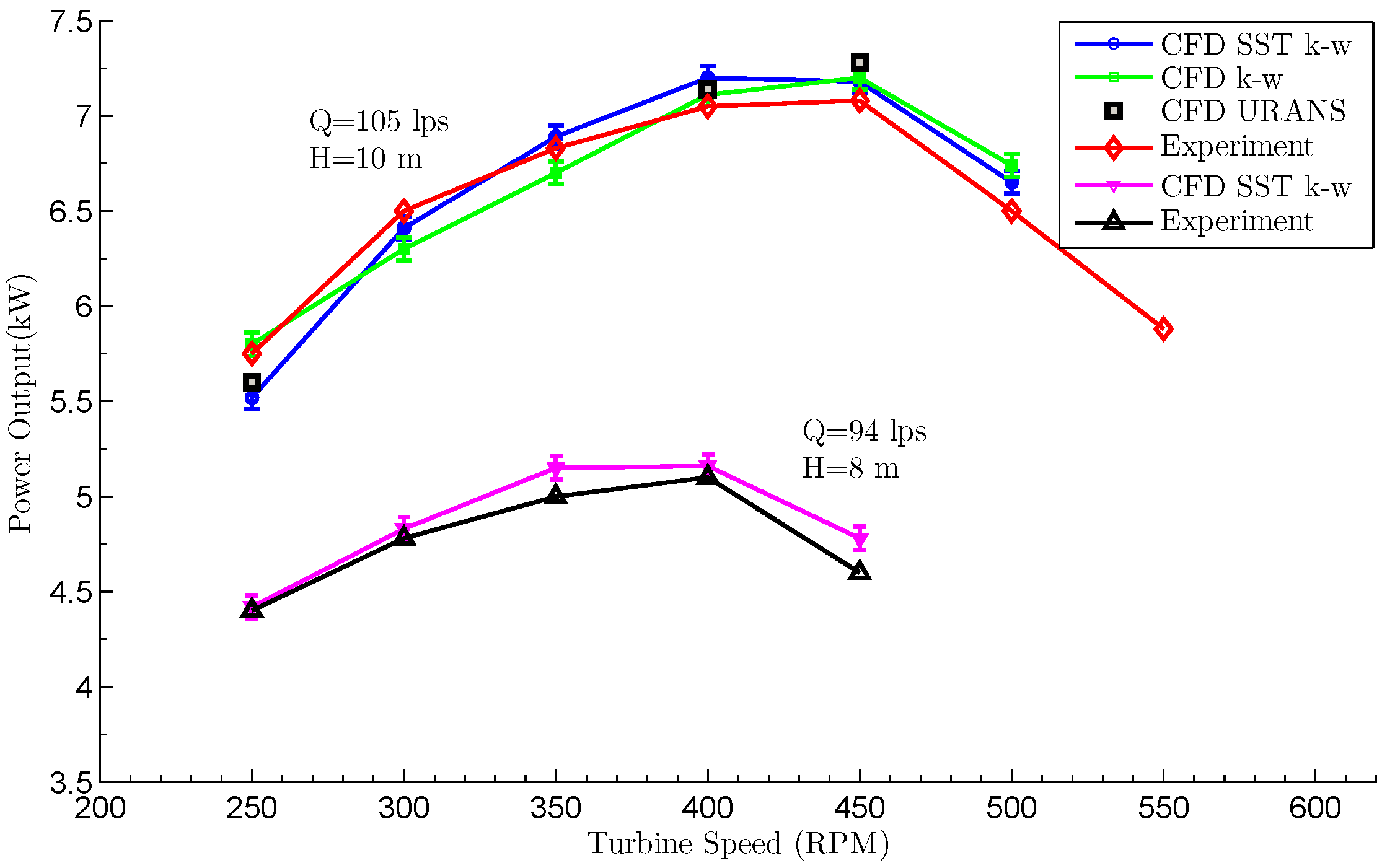
Before examining the main flow features to analyze the inception of cavitation, the predictive capability of the CFD model for the turbine power output was assessed by comparing the CFD results against experimental results. For this, a series of 3D steady and unsteady RANS (URANS) simulations were performed on a small-scale 7 kW crossflow turbine (see Table 1) to examine the inception of cavitation at different Q, H and N. This turbine model was experimentally studied by Dakers and Martin [18] for a range of operating conditions (Q = 56–105 litres per second (lps), H = 3–10 m and N = 200–700 RPM). They obtained a maximum efficiency of 69 % at different values of Q and H. This turbine model was chosen because this is a typical low-head turbine model and all the geometrical details, operating conditions and performance results needed for the CFD analysis are available, which allowed comparison of the CFD results against the experimental results. Comparisons were made for the turbine power output at different Q, H and N corresponding to the experimentally tested conditions (Figure 3). The results showed a satisfactory agreement between the two within the maximum relative error of 6%. The error bars in the CFD results show the numerical uncertainty (0.1%) involved with using the mesh size 5.4 million elements. URANS were also performed in order to determine whether unsteady effects due to impeller motion are significant. This is important because flows in turbines are usually unsteady mainly due to the relative motion or the interactions between the rotating impeller and the stationary nozzle and casing. Steady RANS solutions deal with the unsteadiness associated with turbulence but URANS is needed if there is additional unsteadiness associated with the azimuthal non-uniformity of the nozzle and walls and the impeller. It was found that steady and unsteady RANS computations gave very similar results for the power output, indicating that unsteadiness is not a critical issue and steady simulations could provide satisfactory results. It is therefore assumed here that the two-phase steady RANS solutions are adequate to predict the onset of cavitation and, for brevity, we omit a detailed description of the URANS model. In the foregoing analysis, we have examined the flow field in terms of pressure distributions in the impeller in order to describe the evidence of cavitation inception in the impeller.
4.2. Analysis of the Pressure Field and Cavitation
Since cavitation occurs when the local pressure falls below the vapor pressure of water (3.17 kPa at 25 C), the pressure field in the impeller was examined for evidence of cavitation using Equation (3). The pressure distributions on the impeller blades were examined around the maximum efficiency points for different Q and H. The first series of simulations were performed at Q = 105 lps and H = 10 m at different impeller speeds (N = 400, 450, 500 and 550 RPM) to examine the effects of impeller speed N on the onset of cavitation at constant Q and H. Similarly, the second series of simulations were performed at different Q (94, 73 and 56 lps), H (8, 5 and 3 m) and N (300–450 RPM) to examine the combined effects of reducing Q and H on cavitation inception. Finally, three simulations were performed at different H (8, 10 and 12 m) and keeping Q and N constant at Q = 105 lps and N = 450 RPM respectively to determine the effects of H on cavitation inception. By examining the computed pressure distributions on the blades, cavitation inception was found at several operating conditions.
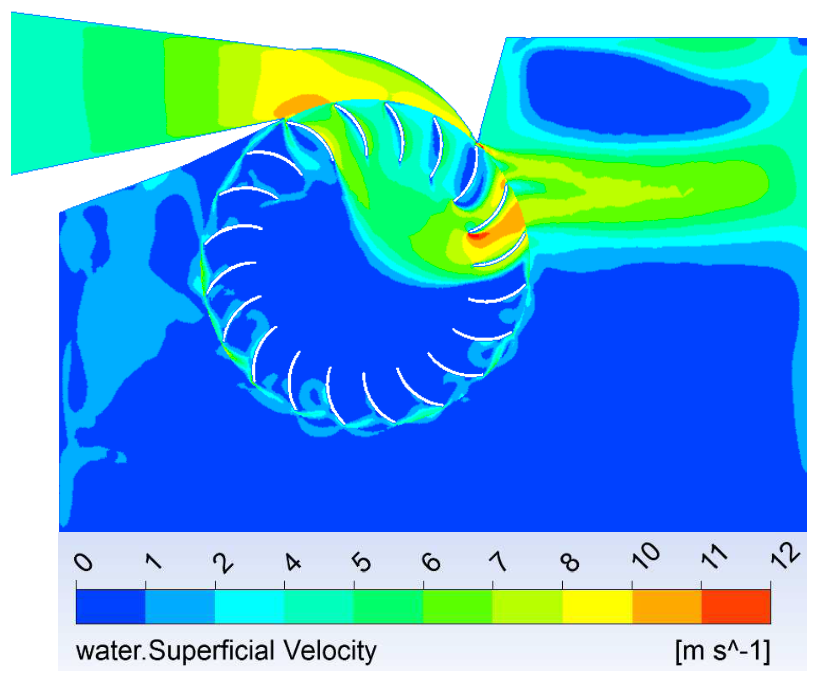
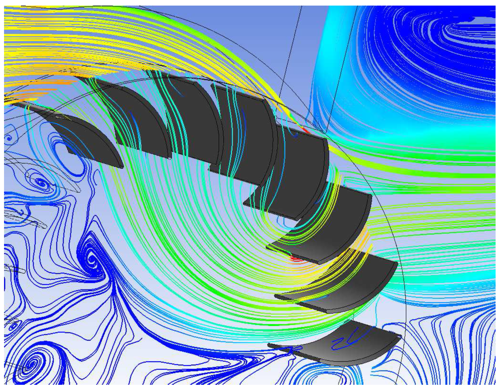
Figure 4 and Figure 5 show the typical main flow path of water and the corresponding streamline patterns in the turbine. As discussed above, power is extracted in two stages. The results of this study show that the blades at the first stage extract most of the fluid power (about 70%), and the blades at the second stage extract the remaining power at a pressure lower than that of the first stage. Therefore, the blades at the second stage are likely the potential regions for cavitation. In all the simulations, cavitation was found only on the blades of the second stage. Cavitation inception was found above the impeller speeds corresponding to maximum efficiency.
The contours of absolute pressure distributions for different Q, H and N are shown in Figure 6, Figure 7 and Figure 8. The examination of the absolute pressure distributions for Q = 105 lps and H = 10 m at different N (400, 450, 500 and 550 RPM) showed that cavitation inception occurred at N = 450 RPM in the second stage. Figure 6 and Figure 7 show that the size of cavitation region has increased with the increase in impeller speed N. A general explanation for these differences is that inertia of the local fluid motion is increased (or reduction in local fluid pressure) with the increase in blade tip-speed as delineated by the Equation (1) and Equation (2). Similarly, pressure distributions at lower Q and H were examined. A comparative analysis of these results showed that the size of cavitation region increased at Q = 94 lps, H = 8 m and N = 450 RPM when compared to the cavitation at Q = 105 lps, H = 10 m and N = 450 RPM or at lower Q and H. As shown in Figure 6 and Figure 7, cavitation inception has occurred at the blade tip on the suction side of one blade at N = 450 RPM and cavitation has increased on the same blade at N = 550 RPM, covering a larger potion of the blade section. At Q = 56 lps and H = 3 m, cavitation was not found at any impeller speed.
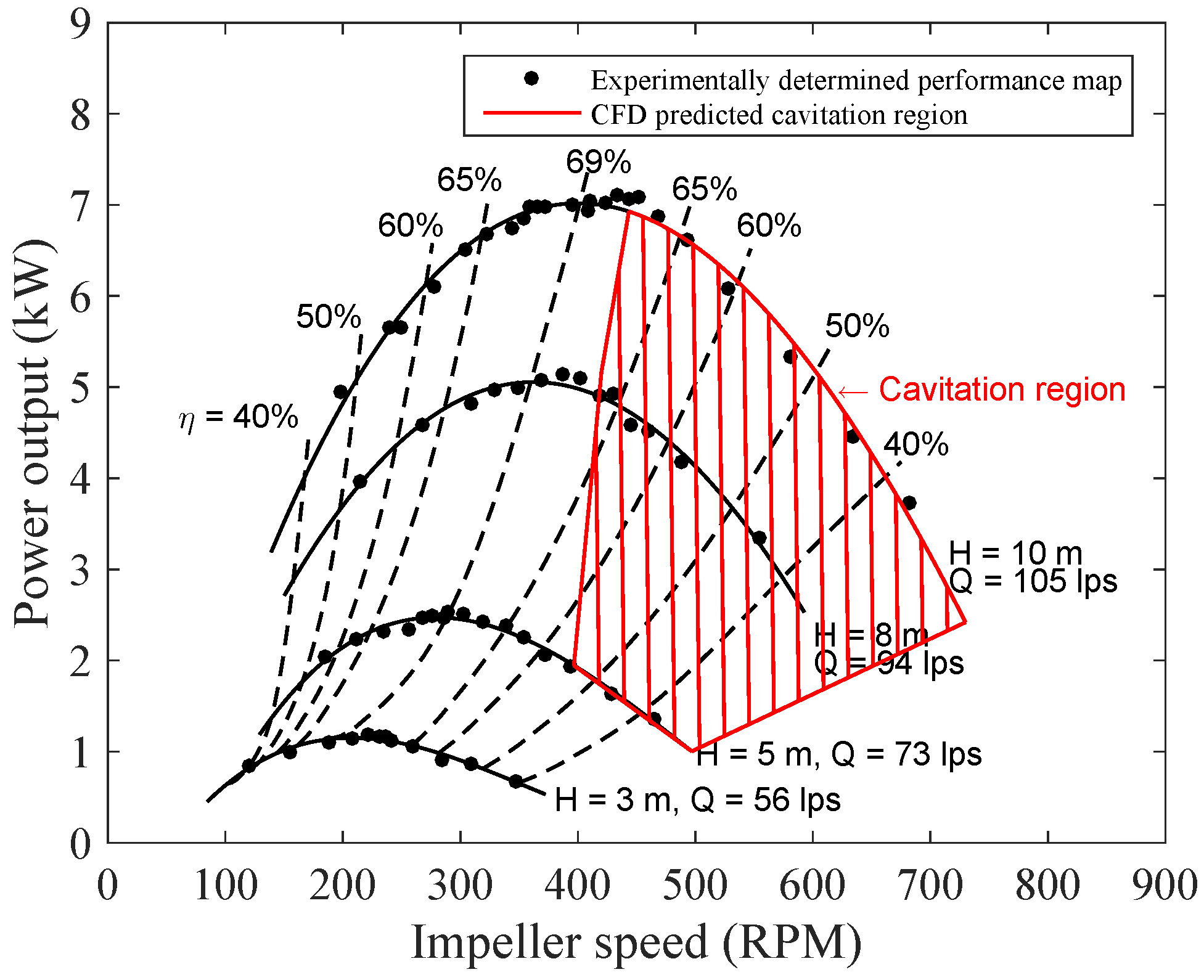
From a practical viewpoint, it is important to establish correlations between cavitation inception and operating parameters, such as Q, H and N. For each Q and H, it is usually desirable to select a suitable impeller speed N to match with the generator speed and to provide efficient operation without cavitation. As discussed in the previous section, the inlet reference pressure or head H is critical in determining the condition for cavitation in the turbine because it affects the cavitation number σ (Equation (1) and Equation (2)). To examine the effects of H on cavitation at Q = 105 lps and N = 450 RPM (corresponding to the maximum efficiency point), three simulations were performed at H = 8, 10 and 12 m. The results showed that cavitation increased with the reduction in H from 10 m to 8 m, whereas cavitation was not found at H = 12 m. The corresponding pressure distributions are shown in Figure 8. The results demonstrate the significance of selecting an appropriate impeller speed N to match the head H and the flow rate Q in order to avoid cavitation. The results of various simulations are summarized in Figure 9 as a performance map of the turbine, which would be useful in selecting the suitable values of Q, H and N to avoid cavitation. The results show that cavitation occurs after the maximum efficiency operating points, which is a highly desirable result. In all the cases considered above, it is noteworthy that the cavitation inception regions are confined to narrow tip regions, primarily on the suction side near the inner edge of the blades at the second stage.
As the flow field contains water and air with free-surface effects, it might be possible that cavitation bubbles are strongly influenced by the air content in the water stream [15]. The air volume fraction may be significant in the water stream in the second row of blades as the flow velocity is reduced at the first stage and the turbine operates at atmospheric condition. A free-surface (water and air interface) can be seen in the second stage as illustrated in Figure 4. It has been shown by previous studies that the erosive power of cavitation due to proximity to a free-surface may be weak [3,15], but there is no guarantee that this weakness occurs for crossflow turbines. This aspect needs further investigation employing a more accurate three-phase and cavitation models and turbulence simulation techniques, such as detached eddy simulation or large eddy simulation to examine the dynamics of pressure field in the multiphase flow.
5. Conclusions
We have shown that cavitation can occur in crossflow turbines. The study was carried out using 3D Reynolds-Averaged Navier–Stokes (RANS) simulations. The flow was modelled as a homogeneous two-phase flow consisting of water and air. A small-scale 7 kW crossflow turbine was analyzed as a reference case for the analysis. The pressure fields in the impeller were examined in order to map the cavitation inception. The main conclusions drawn from this study are summarized below.
In all the operating conditions considered in this study, the onset of cavitation was found to occur only in the second stage of the impeller. The results showed that an increase in the impeller speed increased cavitation at constant flow rate and head. Similarly, increase in head at constant flow rate and impeller speed reduced cavitation. By reducing both the flow rate and head at a constant speed, cavitation increased, reaching a maximum, and then decreased again.
The results of this study have highlighted the significance of cavitation in crossflow turbines. In this work, only the fundamental analysis was performed considering the available computational resources; the size and strength of cavitation bubbles were not studied. A three-phase flow simulation is computationally demanding, whereas a two-phase model is adequate to predict the inception of cavitation. A more detailed investigation (e.g., size and strength of cavitation bubbles and unsteadiness) must be carried out using a three-phase flow model (water, water-vapor and air) if a complete practical explanation or design rules for the design and operation of crossflow turbines need to be developed. We anticipate that this work will stimulate further computational studies in the future. This study is part of an ongoing research project on developing a high-efficiency crossflow turbine; future work will employ a more detailed analysis of cavitation with a focus on developing procedures for cavitation prediction.
Acknowledgments
The authors would like to acknowledge the funding support for this research from NSERC/ ENMAX Research Chair in Renewable Energy at the University of Calgary, Canada. The second author acknowledges the financial support from CNPq, CAPES, Eletronorte and PROPESP/UFPA.
Author Contributions
Ramchandra Adhikari undertook the CFD simulations as part of his PhD research at the University of Calgary, supervised by David Wood. Jerson Vaz formulated the cavitation modelling. All three authors discussed the results and contributed to the explanations of them. The paper was written jointly by all three authors.
Conflict of Interest
The authors declare no conflict of interest. The sponsors had no role in the design of the study; in the collection, analyses, or interpretation of data; in the writing of the manuscript, and in the decision to publish the results.
References
- Michell, A.G.M. Impulse-Turbine, Assigne. U.S. Patent 760898, 24 May 1904. [Google Scholar]
- White, F.M. Viscous Fluid Flow; McGraw-Hill, Inc.: New York, NY, USA, 1991. [Google Scholar]
- Escaler, X.; Egusquiza, E.; Farhat, M.; Avellan, F.; Coussirat, M. Detection of cavitation in hydraulic turbines. Mech. Syst. Signal Process. 2006, 20, 983–1007. [Google Scholar] [CrossRef]
- Mockmore, C.A.; Merryfield, F. The Banki Water Turbine. In Bulletin Series, Engineering Experiment Station; Oregon State System of Higher Education, Oregon State College: Corvallis, OR, USA, 1949. [Google Scholar]
- Durali, M. Design of Small Water Turbine for Farms and Small Communities. Master’s Thesis, Massachusetts Institute of Technology, Cambridge, MA, USA, 1976. [Google Scholar]
- Khosrowpanah, S. Experimental Study of the Crossflow Turbine. Ph.D. Thesis, Colorado State University, Fort Collins, CO, USA, 1984. [Google Scholar]
- Tongco, A.F. Field Testing of a Crossflow Turbine. Ph.D. Thesis, Oklahoma State University, Stillwater, OK, USA, 1988. [Google Scholar]
- Desai, V.R. A Parametric Study of the Cross-Flow Turbine Performance. Ph.D. Thesis, Clemson University, Clemson, SC, USA, 1993. [Google Scholar]
- Aziz, N.M.; Totapally, H.G.S. Design Parameter Refinement for Improved Cross-Flow Turbine Performance; Engineering Report; Department of Civil Engineering, Clemson University: Clemson, SC, USA, 1994. [Google Scholar]
- Nakase, Y.; Fukatomi, J.; Watanaba, T.; Suetsugu, T.; Kubota, T.; Kushimoto, S.A. Study of Cross-Flow Turbine (Effects of Nozzle Shape on Its Performance). In Proceedings of the Winter Annual Meeting, Phoenix, AZ, USA, 14–19 November 1982.
- Choi, Y.; Lim, J.; Kim, Y.; Lee, Y. Performance and internal flow characteristics of a cross-flow hydro turbine by the shapes of nozzle and runner blade. J. Fluid Sci. Technol. 2008, 3, 398–409. [Google Scholar] [CrossRef]
- Andrade, J.; Curiel, C.; Kenyery, F.; AguillÃşn, O.; VÃąsquez, A.; Asuaje, M. Numerical investigation of the internal flow in a Banki turbine. Int. J. Rotating Mach. 2011, 2011. [Google Scholar] [CrossRef]
- Sammartano, V.; AricÚ, C.; Carravetta, A.; Fecarotta, O.; Tucciarelli, T. Banki-Michell Optimal Design by Computational Fluid Dynamics: Testing and Hydrodynamic Analysis. Energies 2013, 6, 2362–2385. [Google Scholar] [CrossRef] [Green Version]
- Brennen, C.E. Fundamentals of Multiphase Flow; Cambridge University Press: New York, NY, USA, 2005. [Google Scholar]
- Batchelor, G.K. An Introduction to Fluid Dynamics; Cambridge University Press: Cambridge, UK, 2000. [Google Scholar]
- Silva, P.A.S.F.; Shinomiya, L.D.; de Olivera, T.F.; Vaz, J.R.P.; Mesquita, A.L.A.; Brasil, A.C.P., Jr. Analysis of cavitation for the optimized design of hydrokinetic turbines using BEM. Appl. Energy 2016, in press. [Google Scholar] [CrossRef]
- ANSYS Academic Research, CFX 15.0 Guide; ANSYS, Inc.: Canonsburg, PA, USA, 2013.
- Dakers, A.J.; Martin, G. Development of a Simple Cross-Flow Water Turbine for Rural Use. In Proceedings of the Conference on Agricultural Engineering, Armidale, Australia, 22–24 August 1982.
- Menter, F.R. Two-Equation Eddy-Viscosity Turbulence Models for Engineering Applications. AIAA J. 1994, 32, 1598–1605. [Google Scholar] [CrossRef]
- Wilcox, D.C. Turbulence Modeling for CFD; DCW Industries: La Canada, CA, USA, 1998. [Google Scholar]
Figure 1.
Geometrical configuration of a crossflow turbine in a small-hydro power system.

Figure 2.
Illustration of pressure distribution on a cavitating blade in the impeller.

Figure 3.
Comparison of computational fluid dynamics (CFD) and experimental results for the turbine power output.
Figure 3.
Comparison of computational fluid dynamics (CFD) and experimental results for the turbine power output.

Figure 4.
A typical velocity contour showing the main flow path of water in the turbine.

Figure 5.
Typical velocity streamlines showing the main flow path of water in the turbine.

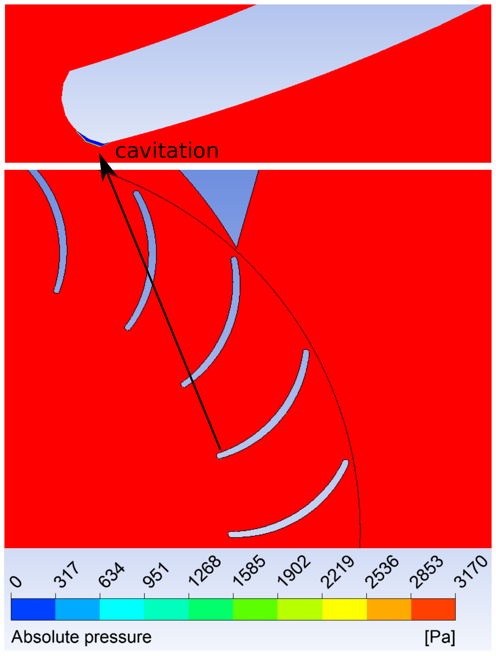
Figure 6.
Contours of pressure distributions on the impeller blades at the second stage (Q = 105 lps and H= 10 m) at the impeller speed 450 RPM, showing the evidence of cavitation inception on the suction sides near the inner edge of the blade.
Figure 6.
Contours of pressure distributions on the impeller blades at the second stage (Q = 105 lps and H= 10 m) at the impeller speed 450 RPM, showing the evidence of cavitation inception on the suction sides near the inner edge of the blade.

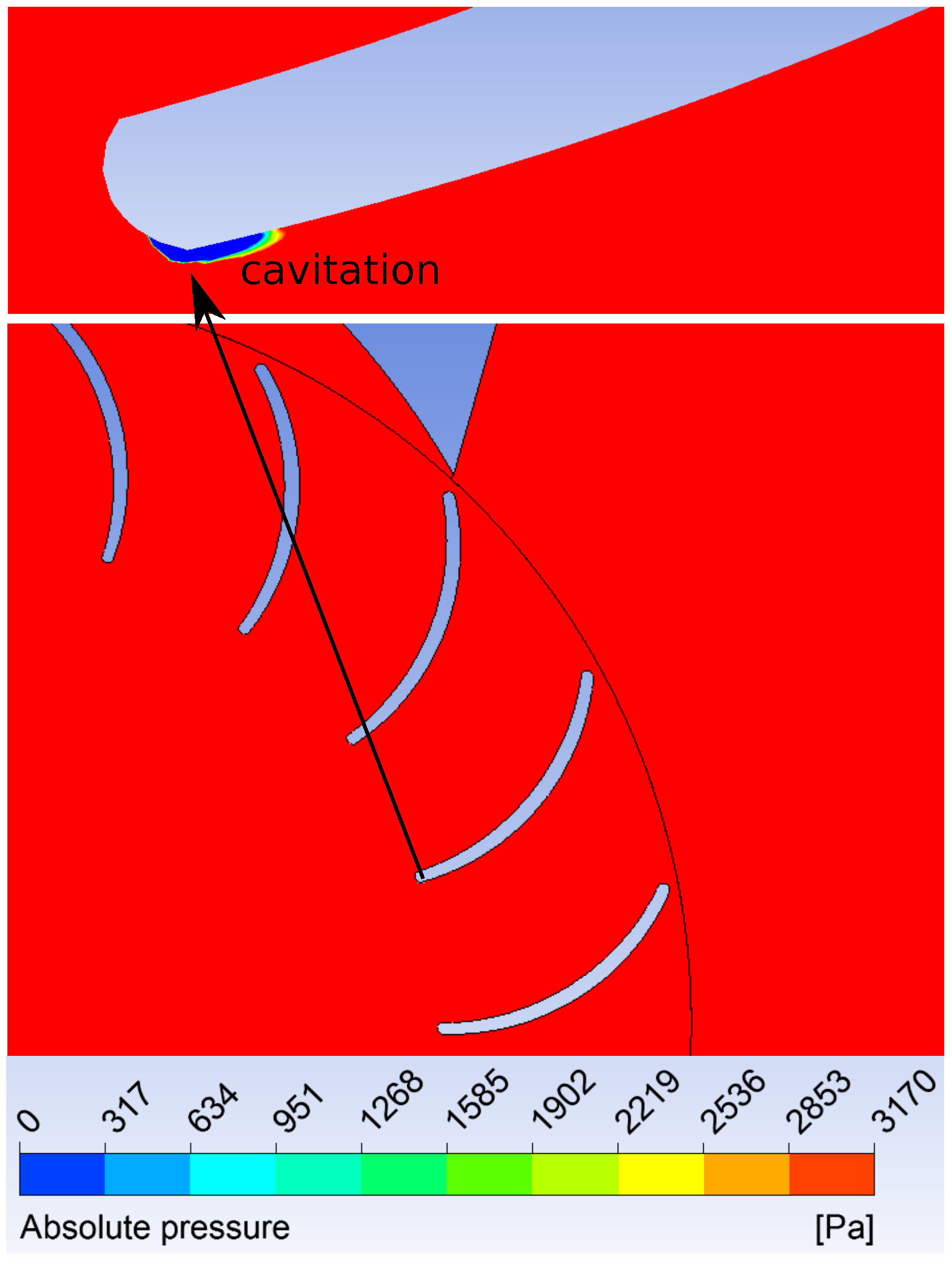
Figure 7.
Contours of pressure distributions on the impeller blades at the second stage (Q = 105 lps and H= 10 m) at the impeller speed 550 RPM, showing the evidence of cavitation inception on the suction sides near the inner edge of the blade.
Figure 7.
Contours of pressure distributions on the impeller blades at the second stage (Q = 105 lps and H= 10 m) at the impeller speed 550 RPM, showing the evidence of cavitation inception on the suction sides near the inner edge of the blade.

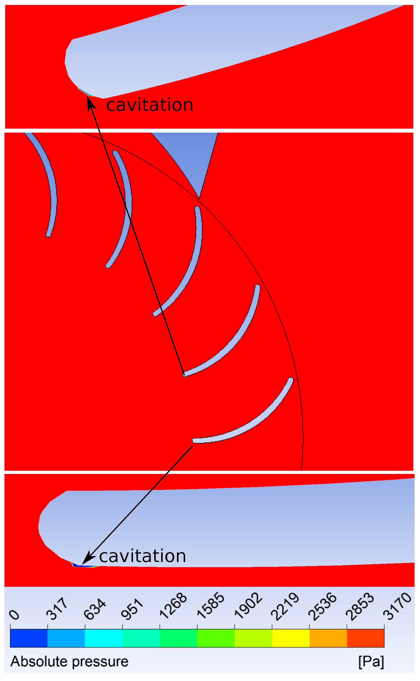
Figure 8.
Contours of pressure distributions on the impeller blades at the second stage at Q = 105 lps, H = 8 m and N = 450 RPM, showing the evidence of cavitation inception on the suction sides near the inner edge of the blades. It is noted that two blades have cavitation at H = 8 m, whereas only one blade has cavitation at H = 10 m.

Figure 9.
CFD predicted cavitation region for the turbine.


Table 1.
Design parameters of the 7 kW turbine [17].
| Design Parameters | Units | Value |
|---|---|---|
| Outer radius () | mm | 158 |
| Inner radius () | mm | 107.4 |
| Angle of attack (α) | 16 | |
| Blade radius () | mm | 52.14 |
| Number of blades | - | 20 |
| Turbine and Nozzle width | mm | 150 |
| Nozzle thickness or throat () | mm | 65 |
| Nozzle outlet arc () | 69 |
| Mesh | No. of Elements | Power Output (kW) | Numerical Uncertainty (%) |
|---|---|---|---|
| Mesh 1 | 2.12 millions | 7.091 | - |
| Mesh 2 | 2.96 millions | 7.122 | 0.43 |
| Mesh 3 | 3.47 millions | 7.157 | 0.49 |
| Mesh 4 | 3.94 millions | 7.169 | 0.16 |
| Mesh 5 | 4.53 millions | 7.181 | 0.16 |
| Mesh 6 | 5.24 millions | 7.192 | 0.15 |
| Mesh 7 | 5.40 millions | 7.199 | 0.10 |
© 2016 by the authors; licensee MDPI, Basel, Switzerland. This article is an open access article distributed under the terms and conditions of the Creative Commons by Attribution (CC-BY) license (http://creativecommons.org/licenses/by/4.0/).
Share and Cite
MDPI and ACS Style
Adhikari, R.C.; Vaz, J.; Wood, D. Cavitation Inception in Crossflow Hydro Turbines. Energies 2016, 9, 237. https://doi.org/10.3390/en9040237
AMA Style
Adhikari RC, Vaz J, Wood D. Cavitation Inception in Crossflow Hydro Turbines. Energies. 2016; 9(4):237. https://doi.org/10.3390/en9040237
Chicago/Turabian StyleAdhikari, Ram Chandra, Jerson Vaz, and David Wood. 2016. "Cavitation Inception in Crossflow Hydro Turbines" Energies 9, no. 4: 237. https://doi.org/10.3390/en9040237
Note that from the first issue of 2016, this journal uses article numbers instead of page numbers. See further details here.