1. Introduction
With the development of photovoltaic (PV) technology or other, similar technologies, renewable energy sources have been used more frequently across the U.S. in recent years. Policies such as renewable portfolio standards (RPS) are gaining more and more attention due to the increasing penetration of renewable energy production into the conventional utility grid. As of March 2015, with 46 states already in session across the country and over 100 RPS bills pending, how to promote solar energy to compete with other major players in the renewable source market is a priority for many solar power producers, utility companies and independent service operators.
The widespread implementations of solar power systems are so far impeded by many factors, such as weather conditions, seasonal changes, intra-hour variability, topographic elevation and discontinuous production. Operators need to acquire solar energy production information ahead of the time to counter the operating costs caused by requirements of energy reserves or shortage of electricity supplies from PV systems. Therefore, solar power forecasting is the “cornerstone” of a reliable and stable solar energy industry. Intra-hour forecasts are critical for monitoring and dispatching purposes while intra-day and day-ahead forecasts are important for scheduling the spinning reserve capacity and managing the grid operations.
The forecast of power output, for example a day ahead, is a challenging task owing to the dependency of inputs’ accuracy. In general, there are two types of inputs for PV energy output forecasting: exogenous inputs from meteorological forecasts, and endogenous inputs from direct system energy outputs. Meteorological forecasts, such as solar irradiance, have been studied for a long time [
1,
2,
3]. Researchers further extended their models to predict power output from PV plants [
4,
5,
6,
7]. However, even with the cloud graph from synchronous meteorological satellites, the large variability in key parameters, namely diffuse component from the sky hemisphere, makes solar irradiance much less predictable than the temperature. More difficulties exist in large-scale PV systems installed over a wide area with different tile and azimuth angles. The situation requires individual parameterized solar models to deal with diverse configurations of PV.
Since it is not possible to take into account all related meteorological forecasts in a practical situation, a lot of alternative solutions have been developed. Some considered adopting weather forecasts provided by meteorological online services [
8]. Many others tried to simplify the solar forecast model by exploring different nonlinear modeling tool such as artificial neural networks (ANN) [
9,
10,
11]. Two types of network, radial basis function (RBF) and multilayer perception (MLP), are commonly utilized to forecast global solar radiation [
12,
13,
14,
15], solar radiation on titled surface [
15], daily solar radiation [
15,
16,
17], and short-term solar radiation [
15,
18]. More techniques are being explored to improve the current models for solar radiation and PV production such as the minimal resource allocating network [
19], the wavelet neural network [
20], fuzzy logic [
21], and the least-square support vector machine [
22]. Others tested PV productions forecasts on reduced weather inputs (e.g., no solar irradiance input) or only based on endogenous inputs [
9,
23,
24]. Proposed approaches include isolating PV linear and nonlinear power outputs [
24], adjusting the temporal resolution [
25], and classified day types [
26,
27,
28,
29].
In this work, a simplified approach, using reduced exogenous inputs without solar irradiance, is developed for predicting the PV production output 15 min, 1 h and 24 h ahead of time. The forecast models, developed from ANN and support vector regression (SVR) respectively, forecast the power output based on PV’s historical record and the online meteorological services. Moreover, an alternative way to forecast total PV output, generated from the individual inverter output forecast, is used to compare the baseline performance using the total PV output data. The goals of this study are to: (1) assess common forecast techniques’ accuracy in order to determine a baseline performance for different prediction windows; (2) propose a hierarchical forecast approach using the monitored information on the inverter level; and (3) validate the approach by comparing the baseline forecasts.
The paper is organized as follows: the next section provides a brief introduction of the methods applied to forecast power plant production;
Section 3 defines the performance matrixes in terms of common error criteria in literatures;
Section 4 gives the data description used in this study; and results are discussed in
Section 5.
3. Performance Matrixes
The performances of the methods described in the previous section are evaluated by several error calculations. For test samples during night hours,
i.e. when solar irradiance is not available, there are no needs to evaluate the system performances. Forecast accuracy is mainly evaluated using the following common statistical metrics:
Mean absolute error (MAE)
Root mean square error (RMSE)
where
is the measured power output,
is the forecasting for
, and
N represents the number of data points which the forecast errors are calculated. MBE is used to estimate the bias between the expected value from predictions and the ground truth. In comparison, MAE provides a view of how close the forecasts are to the measurements in absolute scale. The last one, RMSE, amplifies and severely punishes large errors by using the square form. Although these performance metrics are popular and considered the standard performance measures, limitations with MAE, MBE and RMSE are that the relative sizes of the reported errors are not obvious. It is hard to tell whether they are big or small when comparing to different series of data in different scales. Hence, relative error measures are further introduced:
Mean percentage error (MPE)
Relative root mean squared error (rRMSE)
where
is the maximum power production is recorded, and
is the mean value of solar PV energy production during the daytime in the test period.
is calculated from the below equation:
4. Data
This work uses data collected from a 6 MW (direct current) peak solar power plant with eleven 500 kW (alternative current) inverters located in Florida. This solar farm’s tested period spans from 1 January to 31 December 2014. The intra-hour ground truth data collected from the PV plant site was transferred to 15 min and hourly average of power output. Before applying the training algorithm, both the input and output data are normalized to the range from 0 to 1 using following equation:
where
is the original data value,
is the corresponding normalized value,
is the minimum value in
data set, and
is the maximum value in
data set.
To train the models for different forecasting windows, the primary interest is determining what inputs perform the best at predicting the PV output. The training process is facilitated by testing different configurations of historical power production information. The inputs for the 15 min and 1 h ahead forecast, defined as
H1, is a Markov order 5 sequence:
where
Lt−1 represents historical power plant production from the previous one time step back, …, and
Lt−5 represents production from the previous five time steps back. The 24 h ahead input set, defined as
H2, is used to forecast the next 24 h power production. For one future hour of power production
Lt in the next 24 h window, the input features selected are:
For a one-time-step-ahead forecast (the 15 min and 1 h ahead forecast), inputs include the historical power productions from 1 to 5 time steps back. By comparison, 24 h ahead case needs the historical outputs at the same time from yesterday, the day before yesterday, and so on, until the day one week before. These features are selected based on an exhaustive search by minimizing coefficient of determination.
On the other hand, the reduced exogenous inputs are the following physical variables from weather services: ambient temperature, wind speed, and wind direction. Additional variables are also tried form the National Renewable Energy Laboratory’s SOLPOS (Solar Position and Intensity) calculator as an indirect source to enhance the clear-sky PV production forecast. The following variables were found useful: (1) solar zenith angle, no atmospheric correction; (2) solar zenith angle, degrees from zenith, refracted; (3) cosine of solar incidence angle on panel; (4) cosine refraction corrected solar zenith angle; (5) solar elevation (no atmospheric correction); and (6) solar elevation angle (degrees from horizon, refracted). Various combinations of these variables can be used individually to help to improve the forecasts in different scenarios. This depends on the forecast windows, and these are the all possible variables that can be used. In essence, these additional inputs are adopted as indicators of the clear-sky solar irradiance without explicitly predicting the irradiances. The assumption is that the machine learning algorithms will learn the nonlinear relationship between clear-sky solar properties and the PV plant productions directly rather than through the solar irradiance predictions.
5. Results and Discussion
Two common forecast techniques, ANN and SVR, were tested on the total power production forecast of the sample PV plant. As introduced in
Section 2.3, the traditional baseline forecast uses whole plant production information. It only implements one machine learning model trained with the plant data for power production prediction. The hierarchical method predicts the power production from inverters while each inverter production forecast uses a different machine learning model, which is trained separately based on the information provided by the corresponding inverter only. The summation of these inverter forecasts will transfer micro level predictions to a macro level forecast standing for total plant production.
Table 1,
Table 2 and
Table 3 present forecast results in 2014 for different prediction windows using both approaches. The best results from different error matrixes are highlighted. The hierarchical approach, whether using ANN or SVR, performs better in one step ahead forecast than the traditional way. The 24 h ahead cases are fairly even between the two approaches which is caused by the difficulty of implementing the machine learning algorithms in a longer forecast window, shown by the larger MAE, RMSE and MPE compared to hour-ahead forecast results.
Table 1.
15 min ahead forecast result for the whole photovoltaic (PV) plant. Support vector regression: SVR; mean bias error: MBE; relative MBE: rMBE; mean absolute error: MAE; root mean square error: RMSE; relative RMSE: rRMSE.
Table 1.
15 min ahead forecast result for the whole photovoltaic (PV) plant. Support vector regression: SVR; mean bias error: MBE; relative MBE: rMBE; mean absolute error: MAE; root mean square error: RMSE; relative RMSE: rRMSE.
| Endogenous input | Model | MBE (kWh) | MAE (kWh) | RMSE (kWh) | rMBE | rRMSE | MPE |
|---|
| Inverters | ANN | 0.49 | 34.57 | 42.15 | 0.0131 | 0.131 | 4.32 |
| SVR | 0.58 | 35.73 | 43.52 | 0.0132 | 0.133 | 4.34 |
| Whole plant | ANN | 0.54 | 35.85 | 43.67 | 0.0135 | 0.132 | 4.31 |
| SVR | 0.51 | 36.21 | 45.70 | 0.0132 | 0.135 | 4.31 |
Table 2.
Hour ahead forecast result for the whole PV plant.
Table 2.
Hour ahead forecast result for the whole PV plant.
| Endogenous input | Model | MBE (kWh) | MAE (kWh) | RMSE (kWh) | rMBE | rRMSE | MPE |
|---|
| Inverters | ANN | 0.50 | 51.56 | 63.62 | 0.0128 | 0.134 | 4.32 |
| SVR | 0.55 | 50.77 | 66.87 | 0.0131 | 0.136 | 4.34 |
| Whole plant | ANN | 0.53 | 52.23 | 65.45 | 0.0134 | 0.135 | 4.31 |
| SVR | 0.57 | 54.69 | 65.43 | 0.0131 | 0.135 | 4.31 |
Table 3.
24 h ahead forecast result for the whole PV plant.
Table 3.
24 h ahead forecast result for the whole PV plant.
| Endogenous input | Model | MBE (kWh) | MAE (kWh) | RMSE (kWh) | rMBE | rRMSE | MPE |
|---|
| Inverters | ANN | 0.03 | 126.32 | 182.64 | 0.0001 | 0.410 | 10.54 |
| SVR | 0.05 | 134.48 | 185.44 | 0.0002 | 0.410 | 10.53 |
| Whole plant | ANN | −0.07 | 128.77 | 183.49 | 0.0012 | 0.412 | 10.51 |
| SVR | 0.01 | 126.89 | 185.67 | 0.0002 | 0.411 | 10.52 |
Figure 3 and
Figure 4 display the forecast results comparing the traditional and the hierarchical approach using the same machine learning technique, such as ANN. In
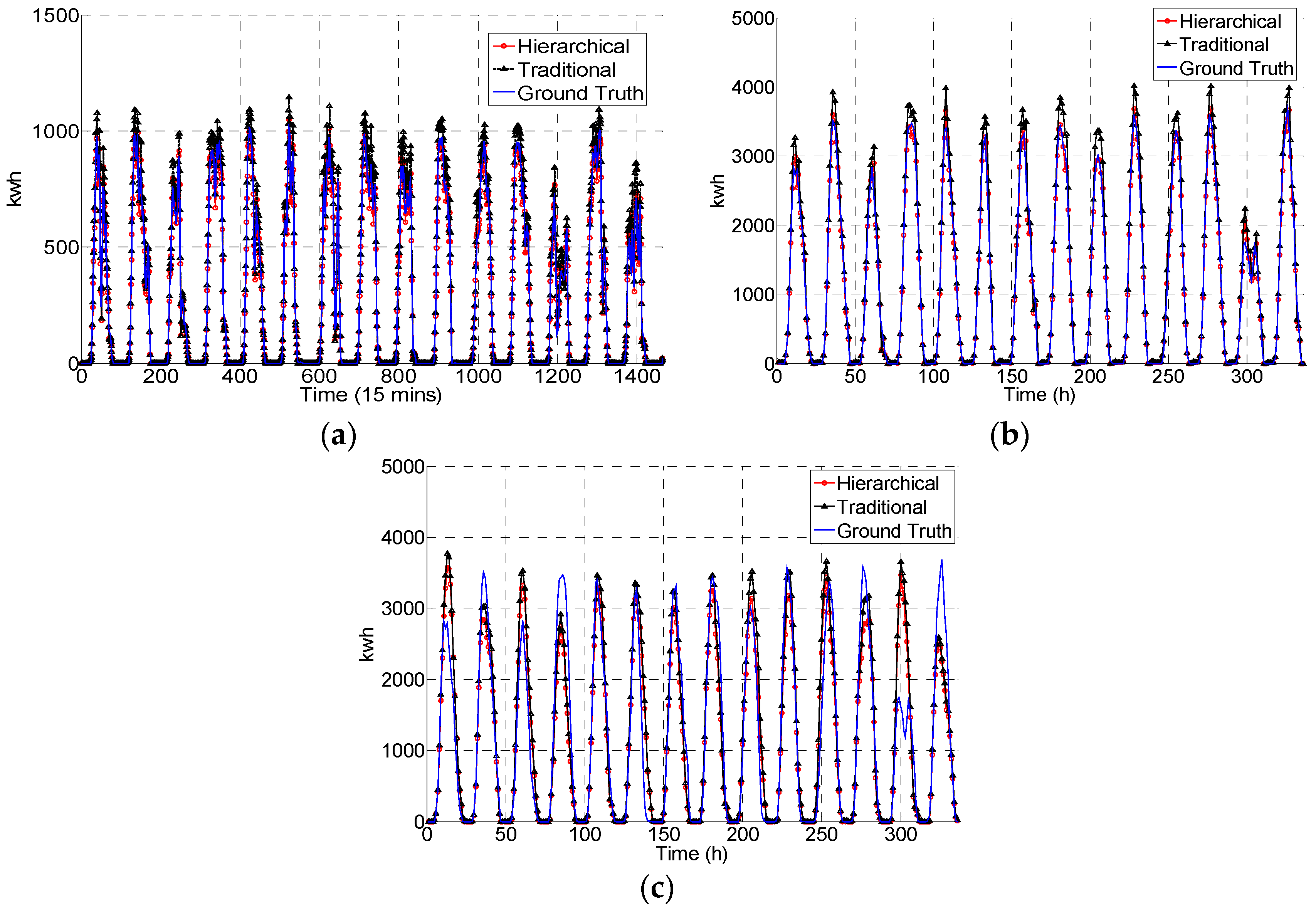
Figure 3, the presented two-week period shows improvements in performance using the hierarchical approach for forecasts 15 min, 1 h and 24 h ahead. In particular, we observe a strikingly difference results for the 24 h ahead case from the consistent performances for 15 min and 1 h forecasts, which are the cases one time step ahead. Power production forecasting plots in
Figure 3a,b, even on the cloudy day (around 1200 time steps in the 15 min ahead plot and 300 time steps in the hour ahead plot), match the ground truth pattern with a low error. In contrast, the same case in the 24 h forecast apparently excessively predicts the true power production. The dampened performance for the 24 h case is clearly influenced by the input features. In the 24 h ahead forecast, models learned the patterns as a daily profile which is a 24 time steps ahead of the moving window. The key assumption behind the learning process is that daily power plant production levels are similar without large deviation, which may not be the case for all days. That is why cloudy or rainy weather factors play more important roles than historical power production information in 24 h ahead cases. However, due to the goals and definitions of the approaches, the factors cannot be easily approximated from the reduced exogenous inputs in our study. Besides the 24 h tests, 15 min and 1 h ahead predictions actually do not depend too much on exogenous inputs. Sample plots for rainy and cloudy days’ forecasts in
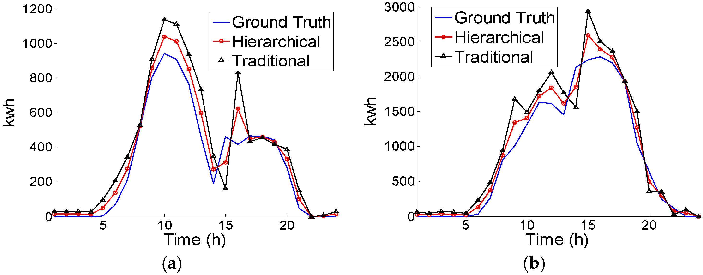
Figure 4 indicate that the trained model with endogenous inputs can predict the plant power production for one time step ahead with an appropriate error level. On the cloudy day, the production level of energy is affected by the cloudy periods and changes can be observed from 10 am to 3 pm in
Figure 4a. In comparison, the rainy day has more irregular productions in the entire daytime, and more periods are either over-fitted or under-estimated (e.g., the periods from 2 pm to 4 pm).
Figure 3.
The forecast results comparison over a two-week period. (a) 15 min forecasts; (b) 1 h forecast; and (c) 24 h forecast.
Figure 3.
The forecast results comparison over a two-week period. (a) 15 min forecasts; (b) 1 h forecast; and (c) 24 h forecast.
Figure 4.
Sample plots for a (a) rainy and (b) cloudy day.
Figure 4.
Sample plots for a (a) rainy and (b) cloudy day.
Table 4 and
Table 5 list all the inverter values for the 15 min and 1 h ahead forecast windows using ANN. The classification of the inverter groups are based on plant configuration and areas occupied. The similar size for the plant inverter guarantees a comparative view on which areas have the most potential in production predictions and which inverter causes the most trouble in power forecasting.
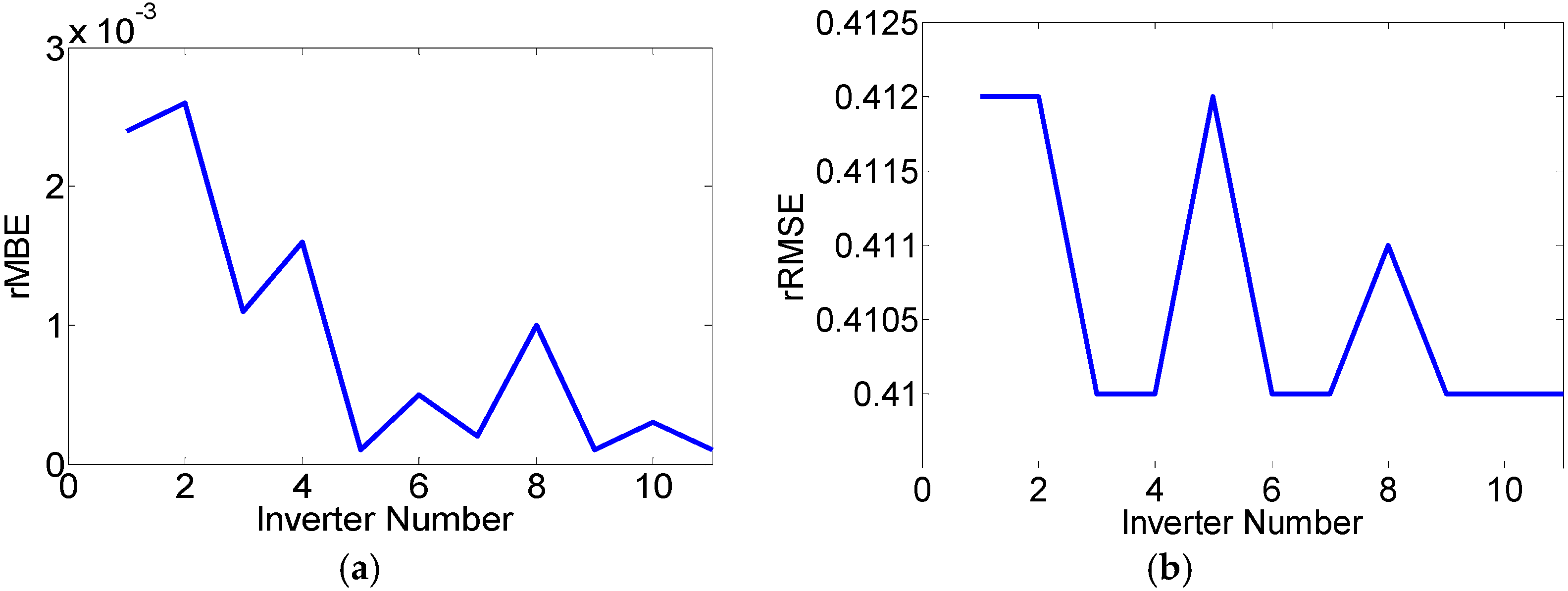
Table 6 further illustrates the effects of the hierarchical approach while predicting power plant production from the micro level to a macro analysis. In terms of MBE, the unstable error implies similar chances to overly predict or inadequately predict the power output regardless of the power production levels. The evaluations based on absolute changes, such as MAE, MPE and RMSE, represent the evolving process when the power production level increases with the max energy shown as well. The gradually improved forecasts are measured by rMBE and rRMSE. By comparing the total summation form 11 inverter predictions and the forecast using the historical power production from the whole plant, we can conclude that the hierarchical approach performs better in terms of MBE, MAE, RMSE, rMBE, and rRMSE, which is shown in
Figure 5.
Table 4.
15 min forecast results for each inverter.
Table 4.
15 min forecast results for each inverter.
| Inverter | MBE (kWh) | MAE (kWh) | RMSE (kWh) | rMBE | rRMSE | MPE | Max energy (kWh) |
|---|
| A1 | −0.57 | 4.95 | 6.15 | 0.0124 | 0.134 | 4.36 | 113.4 |
| A2 | −0.55 | 5.06 | 6.27 | 0.0118 | 0.134 | 4.39 | 113.15 |
| B1 | −0.52 | 4.93 | 6.13 | 0.0112 | 0.131 | 4.39 | 110.45 |
| B2 | −0.39 | 5.03 | 6.24 | 0.0083 | 0.133 | 4.45 | 111.16 |
| C1 | 0.42 | 4.91 | 6.11 | 0.0119 | 0.133 | 4.42 | 110.45 |
| C2 | 0.51 | 4.97 | 6.19 | 0.0126 | 0.133 | 4.37 | 109.75 |
| D1 | 0.45 | 5.09 | 6.21 | 0.0133 | 0.134 | 4.46 | 110.5 |
| D2 | 0.56 | 5.14 | 6.15 | 0.0148 | 0.132 | 4.41 | 110.25 |
| E1 | −0.57 | 4.96 | 6.18 | 0.0134 | 0.131 | 4.36 | 112.89 |
| E2 | 0.43 | 5.07 | 6.22 | 0.0127 | 0.131 | 4.43 | 112.5 |
| E3 | 0.44 | 5.03 | 6.26 | 0.0131 | 0.134 | 4.37 | 114.2 |
Table 5.
1 h forecast result for each inverter.
Table 5.
1 h forecast result for each inverter.
| Inverter | MBE (kWh) | MAE (kWh) | RMSE (kWh) | rMBE | rRMSE | MPE | Max energy (kWh) |
|---|
| A1 | 0.59 | 4.55 | 5.58 | 0.0146 | 0.139 | 4.08 | 446 |
| A2 | 0.48 | 4.69 | 5.74 | 0.0118 | 0.140 | 4.14 | 452.6 |
| B1 | 0.44 | 4.62 | 5.63 | 0.0107 | 0.137 | 4.18 | 441.8 |
| B2 | 0.47 | 4.71 | 5.74 | 0.0114 | 0.140 | 4.24 | 444.64 |
| C1 | 0.49 | 4.75 | 5.55 | 0.0127 | 0.135 | 4.19 | 441.8 |
| C2 | 0.55 | 4.63 | 5.62 | 0.0119 | 0.140 | 4.26 | 439 |
| D1 | 0.43 | 4.62 | 5.72 | 0.0125 | 0.139 | 4.19 | 442 |
| D2 | 0.52 | 4.59 | 5.67 | 0.0141 | 0.138 | 4.20 | 441 |
| E1 | 0.58 | 4.58 | 5.56 | 0.0135 | 0.137 | 4.16 | 451.56 |
| E2 | 0.50 | 4.68 | 5.63 | 0.0133 | 0.138 | 4.22 | 450 |
| E3 | 0.55 | 4.70 | 5.66 | 0.0129 | 0.136 | 4.21 | 456.8 |
Table 6.
24 h forecast result for different number of inverters.
Table 6.
24 h forecast result for different number of inverters.
| Inverter | MBE (kWh) | MAE (kWh) | RMSE (kWh) | rMBE | rRMSE | MPE | Max energy (kWh) |
|---|
| 1 | −0.10 | 11.46 | 16.37 | 0.0024 | 0.412 | 10.28 | 446 |
| 2 | −0.21 | 23.39 | 33.13 | 0.0026 | 0.412 | 10.41 | 898.6 |
| 3 | −0.14 | 35.27 | 49.73 | 0.0011 | 0.410 | 10.52 | 1340.4 |
| 4 | −0.25 | 47.19 | 66.40 | 0.0016 | 0.410 | 10.57 | 1785.04 |
| 5 | 0.01 | 58.95 | 83.09 | 0.0001 | 0.412 | 10.59 | 2226.84 |
| 6 | 0.11 | 70.11 | 99.08 | 0.0005 | 0.410 | 10.52 | 2665.84 |
| 7 | 0.06 | 81.96 | 115.80 | 0.0002 | 0.410 | 10.55 | 3107.84 |
| 8 | −0.31 | 93.43 | 132.07 | 0.0010 | 0.411 | 10.53 | 3548.84 |
| 9 | 0.03 | 105.58 | 149.10 | 0.0001 | 0.410 | 10.56 | 4000.4 |
| 10 | 0.11 | 117.27 | 165.70 | 0.0003 | 0.410 | 10.54 | 4450.4 |
| 11 | 0.03 | 126.32 | 182.64 | 0.0001 | 0.410 | 10.54 | - |
| Whole plant | −0.07 | 128.77 | 183.49 | 0.0002 | 0.412 | 10.51 | - |
Figure 5.
The hierarchical approach in terms of evolving errors: (a) rMBE and (b) rRMSE.
Figure 5.
The hierarchical approach in terms of evolving errors: (a) rMBE and (b) rRMSE.
The evolving process of the hierarchical approach shows the potential to have multiple-level forecasts of the PV system, and they can be used for various purposes such as optimization of the production schedules at the inverter level and micro controls for multiple solar modules in a large PV system.
6. Conclusions
This work compares two common models, ANN and SVR, for 15 min, 1 h and 24 h forecasting of the averaged power output of a 6 MWp PV power plant. No exogenous data such as solar irradiance was used in the forecasting models. A hierarchical approach using micro level information on the power plant, such as inverters, is further assessed. From the analysis of the error between ground truth and predicted values, it can be concluded that hierarchical technique outperforms traditional models using power production information from the micro level of the plant system. In addition, we discuss and show the difference between a one-step-ahead forecast, namely 15 min and 1 h ahead, and a 24 h forecast using both approaches. The analysis of the evolving errors, calculated by the summation of the different inverter number, shows the potential of the hierarchical approach to determine which smaller generation units have the greatest impact on forecasting.


