Power Quality Prediction, Early Warning, and Control for Points of Common Coupling with Wind Farms

Abstract

Wind farms can affect the power quality (PQ) of the power supply grid, with subsequent impacts on the safe and stable operation of other electrical equipment. A novel PQ prediction, early warning, and control approach for the common coupling points between wind farms and the network is proposed in this paper. We then quantify PQ problems and provide rational support measures. To obtain predicted PQ data, we first establish a trend analysis model. The model incorporates a distance-based cluster analysis, probability distribution analysis based on polynomial fitting, pattern matching based on similarity, and Monte Carlo random sampling. A data mining algorithm then uses the PQ early warning flow to analyze limit-exceeding and abnormal data, quantify their severity, and output early warning prompts. Finally, PQ decision support is applied to inform both the power suppliers and users of anomalous changes in PQ, and advise on corresponding countermeasures to reduce relevant losses. Case studies show that the proposed approach is effective and feasible, and it has now been applied to an actual PQ monitoring platform.

1. Introduction

As a renewable, green resource, wind power has the potential to make a remarkable contribution to mitigating future energy crises and reducing greenhouse gas emissions. Hence, wind farms continue to grow at a significant pace across the world [1]. However, wind power is random, intermittent, and volatile, and wind farms use many electronic devices to access the power grid. Inevitably, these bring about a certain degree of power quality (PQ) pollution [2,3,4,5]. It usually includes both harmonics and voltage deviations. In different systems, PQ problems will become different. When the wind turbine connects to the grid, current harmonics may also happen. When the wind turbine operates in island, voltage harmonics, voltage fluctuation, flicker and power fluctuation may also occur. Some serious PQ problems may affect the safe and stable operation of other electrical equipment and the whole power supply grid. At the same time, economic and social development has led to power users demanding greater PQ. Therefore, it is necessary to analyze and quantify the severity of PQ problems so that effective countermeasures can be taken [6,7].

To date, many studies have focused on analyzing PQ characteristics of points of common coupling (PCCs) with wind farms. Furthermore, most PQ research concentrates on the assessment, detection, identification, location, and improvement of PQ [8,9,10,11,12,13,14]. PQ assessment can be used to make comprehensive judgments on the status of PQ over a historical period, but it fails to assess PQ status in the future. The goal of PQ detection is to identify PQ disturbance from many signals. The methods have a good ability to carry out signal recognition, but they are accustomed to already-existing PQ analysis problems. PQ location methods can be used to locate PQ disturbances quickly and accurately, but it also analyzes historical data. There are many measures that can be used to improve PQ, and the control effects are satisfactory. However, these measures are rarely combined with trend analysis and early warnings.

From the above analysis, there is little research on PQ trend analysis, early warning systems for PQ anomalous changes, or the provision of the corresponding decision support. However, certain previous studies provide the necessary background for the work described in this paper [15,16]. The proposed approach has the following contributions: (1) Such techniques enable power supply companies, whose monitored PQ data are obtained at some time lag and can only reflect historical PQ changes, to identify hidden PQ problems in advance and make adjustments to improve the reliability and quality of the power supply. This will clearly influence the real-time scheduling and control of the whole power grid; (2) The greatest concern of most wind farms is safe and stable operation, with PQ problems of secondary importance. Although wind farms can monitor PQ data by installing suitable equipment, some improved PQ measures operate at a delay and cannot be put to work immediately. PQ trend analysis helps wind farms realize PQ changes and plan ahead to adjust their operations. Operators may also be able to switch control measures to improve PQ and form a basis for fixing the electricity price based on PQ.

The rest of this paper is organized as follows: Section 2 gives a brief introduction to PQ prediction, before Section 3 presents the proposed PQ trend early warning approach. Section 4 describes our method for PQ decision support. In Section 5, we discuss the implementation of the proposed approach, and case studies are presented in Section 6. Finally, our conclusions are duly drawn in Section 7.

2. Power Quality (PQ) Prediction Approach

To analyze PQ, it is necessary to identify and predict certain trends, particularly those circumstances that can cause PQ anomalies during the actual operation of the wind farm and the power supply grid. Based on historical monitored PQ data and the corresponding experimental data, this paper presents a trend analysis approach. First, to improve the accuracy of the monitored data analysis, the distances between different samples are computed to enable a cluster analysis to be performed. The polynomial fitting method is then used to calculate the probability distributions of different categories. Next, similarity-based pattern matching identifies the sample that best matches the specified parameters. Finally, a Monte Carlo algorithm is used to generate random samples for data prediction. The analysis is performed as follows.

2.1. Cluster Analysis Based on Dynamic Time Warping (DTW) Distance

To improve the efficiency with which PQ data is used, we employ cluster analysis to classify data on the basis of similarity. This is an exploratory data analysis method, without direct instruction or supervision. At present, there are many cluster analysis techniques, such as density-based, grid-based, and model-based methods [17,18]. This study uses a distance-based approach. Specifically, the dynamic time warping (DTW) algorithm is used to classify data.

On the basis of dynamic programming, DTW is a nonlinear technology that can combine time and distance measures to find the minimum bending path between two time sequences [19,20].

Let the reference time sequence be R = (r₁, r₂, …, r_m)^T and the test time sequence be T = (t₁, t₂, …, t_n)^T. The time warping function is then defined as:

$$C=\{c(1),c(2),\dots ,c(N)\}$$

(1)

where N is the path length, and c(k) = (i(k), j(k)) represents the matching point pair consisting of statistic features i(k) and j(k). Their distance can be called the local matching distance. The minimum bending path between T and R can be calculated as:

$$D=\min {\displaystyle \sum _{k=1}^N[d(a_{i(k)},b_{j(k)})]}$$

(2)

To make the dynamic path search more practical, we must add some restrictions:

$$\{\begin{array}{l}\max (m,n)\le k\le m+n-1\\ c_1=d_{11},c_m=d_{mn}\\ 0\le i-i^{\prime }\le 1,0\le j-j^{\prime }\le 1\end{array}$$

(3)

where c_k = d_ij; c_k−1 = d_i′j′.

Based on this formulation, our cluster analysis based on the DTW distance is implemented as follows:

(1) Consider monitored PQ data from one day as a sample set, and compute the DTW distance between two samples.

(2) Determine the threshold for cluster analysis based on experience. If the DTW distance between two samples is less than the threshold, they are placed in the same category.

(3) Continue parsing all samples to complete the cluster analysis.

2.2. Probability Distribution Analysis Based on Polynomial Fitting

Probability distributions are used to describe the likelihood of random variables occurring. If the number of samples is sufficiently high, the frequency function of an event can be regarded as its probability distribution. Based on this principle, the probability that sample data belongs to the same category can be computed.

Polynomial fitting can then be used to compute the probability distribution function [21]. The polynomial fitting method is a data fitting technique that aims to determine:

$$p_n(x)={\displaystyle \sum _{k=0}^n{a}_k{x}^k}\in \varphi$$

(4)

where n is the polynomial degree, a_k are the polynomial coefficients, and Φ is the function class composed of polynomials (whose degrees are less than the given number of points), such that the following holds:

$$I={\displaystyle \sum _{i=0}^m{[p_n(x_i)-y_i]}^2}={\displaystyle \sum _{i=0}^m{[{\displaystyle \sum _{k=0}^n{a}_k{x}^k}-y_i]}^2}=\min$$

(5)

where x_i and y_i are given points, m is the number of given points, and I represents the error between the true value and the computed value.

p_n(x) is the so-called least-squares method for a polynomial, and it can be seen as a linear fitting or line fitting when n = 1. In practical applications, n ≤ m; when n is equal to m, the fitting polynomial is the Lagrange or Newton interpolation polynomial.

2.3. Pattern Matching Based on Similarity

Pattern matching aims to find the correspondence between two input patterns. This study will examine the link between test data and sample data, which represent predicted data and historical monitored data, respectively. Based on this pattern matching, the sample in the database that best matches the test data can be found. Then, according to the relationship between the sample data and the derived probability distribution, the corresponding polynomial distribution is assigned to the test data.

This paper uses a similarity algorithm based on DTW to perform pattern matching. After computing the DTW distance on the basis of the method described in Section 2.1, the similarity between the test data and the samples in the database is calculated as:

$$s(T,R)=\frac{90}{90+D(T,R)}\times 100\%$$

(6)

where s(T, R) represents the similarity between the time sequences T and R, and high values of s(T, R) correspond to higher similarity; D(T, R) denotes the DTW distance between time sequences T and R.

The probability distribution corresponding to the minimum similarity is then extracted from the database.

2.4. Random Sampling Using a Monte Carlo Method

Monte Carlo methods use random samples to answer questions of interest [22]. Random values of between 0 and 1 are generated according to a specified distribution. The probability distribution analyzed in this paper is nonstandard, so we cannot produce random data in the usual manner.

To solve this problem, we use a dichotomy method to translate the production of random data into a multinomial distribution.

The random data are generated as follows:

(1) A Monte Carlo method is used to generate random values between 0 and 1, and these are regarded as the dependent variable of the probability distribution function.

(2) The inverse of the probability distribution function is computed. Using the above dependent variable as the independent variable, values of the inverse function can be computed. These are the random data values required by this study.

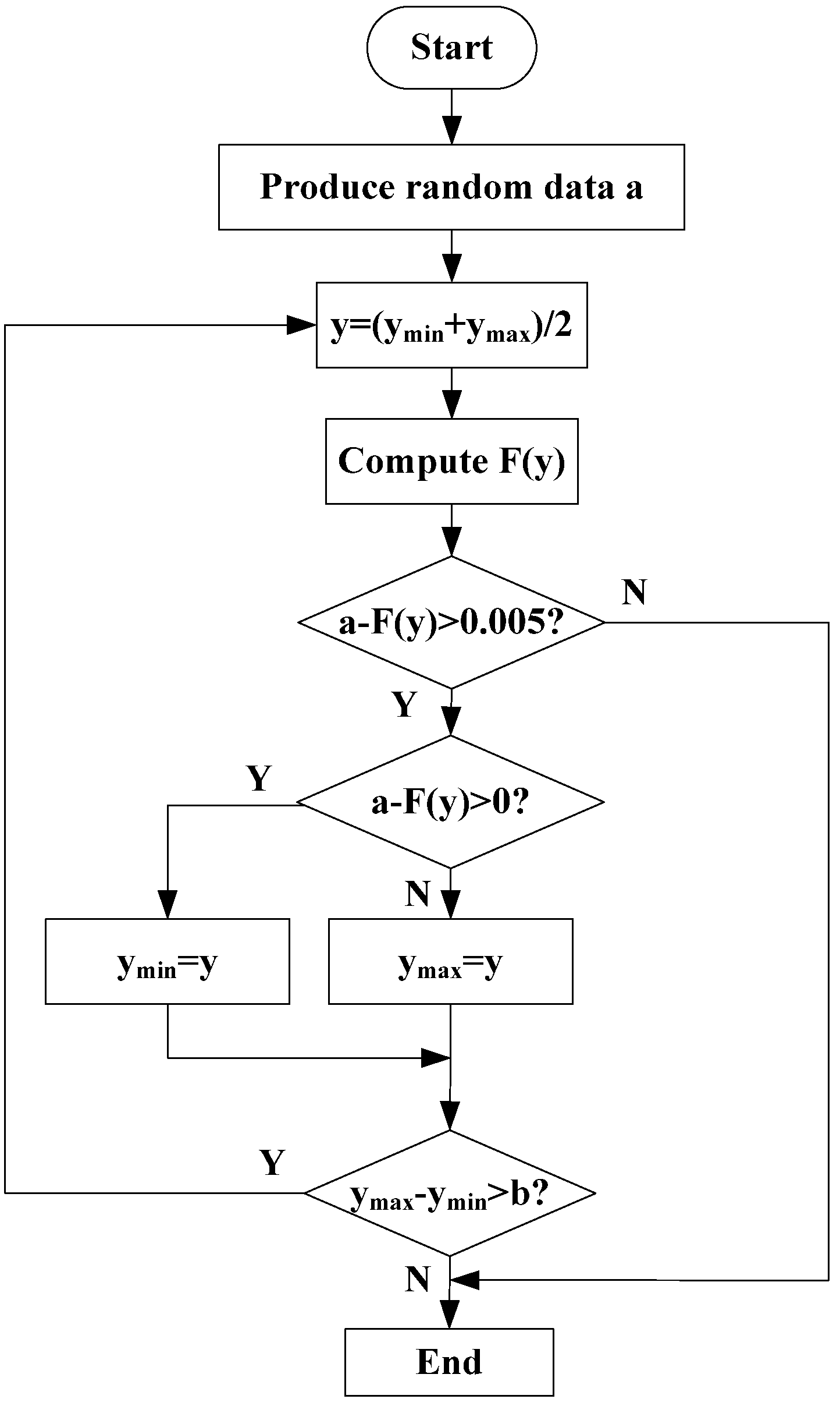
However, when polynomial fitting is used to calculate the probability distribution for actual analysis, it may be difficult to compute the inverse function. To solve this problem, the dichotomy method is used to produce random data. A flowchart illustrating the production of random data is shown in Figure 1.

Finally, the data sampled by the above method can be considered as predicted PQ trend data.

Figure 1. Flowchart for the production of random data.

Figure 1. Flowchart for the production of random data.

3. PQ Early Warning Approach

Following the process of trend analysis, predicted PQ data can be obtained. It is useful to analyze limit-exceeding and abnormal information within these data to provide rational early warning prompts. These prompts enable both the power suppliers and users to realize the severity of PQ problems and take appropriate countermeasures [23].

Following [24], we consider the flow at three levels and four grades to produce PQ early warnings. First, a limit-exceeding detection should be carried out. The number of data that exceed the national standard limits can be calculated and compared with the thresholds for Grades 4 or 3 to judge whether it is necessary to output a limit-exceeding early warning.

If the number of limit-exceeding data is below the threshold for Grade 3, a 95% probability value detection should be implemented. To obtain the 95% probability value, the monitored data need to be listed in descending order. Then, the top 5% can be removed. Furthermore, the maximum of the remaining data is the 95% probability value detection [25]. Similar to a limit-exceeding detection, the 95% probability value can be compared with the thresholds for Grades 3 or 2 to judge the required grade of early warning.

If the 95% probability value falls below the threshold for Grade 2, anomaly detection should be implemented. During this process, the skewness and kurtosis of higher-order statistics can be used to detect a status change.

Skewness measures the direction and degree of skew in statistical data. Its value reflects the degree of asymmetry in a probability density curve relative to the average [24,26]. The skewness is given by:

$$s_k=\{\begin{array}{l}0,\\ \{-\frac{\sqrt{\mathrm{var}(g_1)}}{\sqrt{a}}\le g_1\le \frac{\sqrt{\mathrm{var}(g_1)}}{\sqrt{a}}\}\\ g_1=\frac{N\cdot {\displaystyle \sum _{n=1}^N{(x(n)-m)}^3}}{(N-1)\cdot (N-2)\cdot {(\text{σ})}^3},\\ \text{{}-\infty \le g_1\le -\frac{\sqrt{\mathrm{var}(g_1)}}{\sqrt{a}},\frac{\sqrt{\mathrm{var}(g_1)}}{\sqrt{a}}\le g_1\le +\infty \text{}}\end{array}$$

(7)

where x = {x(n): n = 1, 2, …, N}; g₁ is its unbiased estimate; m and σ are the average and standard deviation of x(n), respectively; and a = 1− q (q generally takes the value 0.95). The variance of g₁ is:

$$\mathrm{var}(g_1)=\frac{6\cdot N\cdot (N-1)}{(N-2)\cdot (N+1)\cdot (N+3)}$$

(8)

Kurtosis describes the peak value when the probability density curve is situated at the average point. In short, it reflects the degree of steepness of all variate distribution values [24,26]. The kurtosis is computed as follows:

$$k_u=\{\begin{array}{l}\frac{-6}{N-1},\\ \{\frac{-6}{N-1}-\frac{\sqrt{\mathrm{var}(g_2)}}{\sqrt{a}}\le g_2\le \frac{-6}{N-1}+\frac{\sqrt{\mathrm{var}(g_2)}}{\sqrt{a}}\}\\ g_2\text{=}\frac{N\cdot (N+1)\cdot {\displaystyle \sum _{n=1}^N{(x(n)-m)}^4}}{(N-1)\cdot (N-2)\cdot (N-3){(\text{σ})}^4}-\frac{3\cdot {(N-1)}^2}{(N-2)\cdot (N-3)},\\ \text{{}-\infty \le g_2\le \frac{-6}{N-1}-\frac{\sqrt{\mathrm{var}(g_2)}}{\sqrt{a}},\frac{-6}{N-1}+\frac{\sqrt{\mathrm{var}(g_2)}}{\sqrt{a}}\le g_2\le +\infty \text{}}\end{array}$$

(9)

where x = {x(n): n = 1, 2, …, N}; g₂ is its unbiased estimate; m and σ are the average and standard deviation of x(n), respectively; and a = 1− q (q generally takes the value 0.95). The variance of g₂ is:

$$\mathrm{var}(g_2)=\frac{24\cdot N\cdot {(N-1)}^2}{(N-3)\cdot (N-2)\cdot (N+3)\cdot (N+5)}$$

(10)

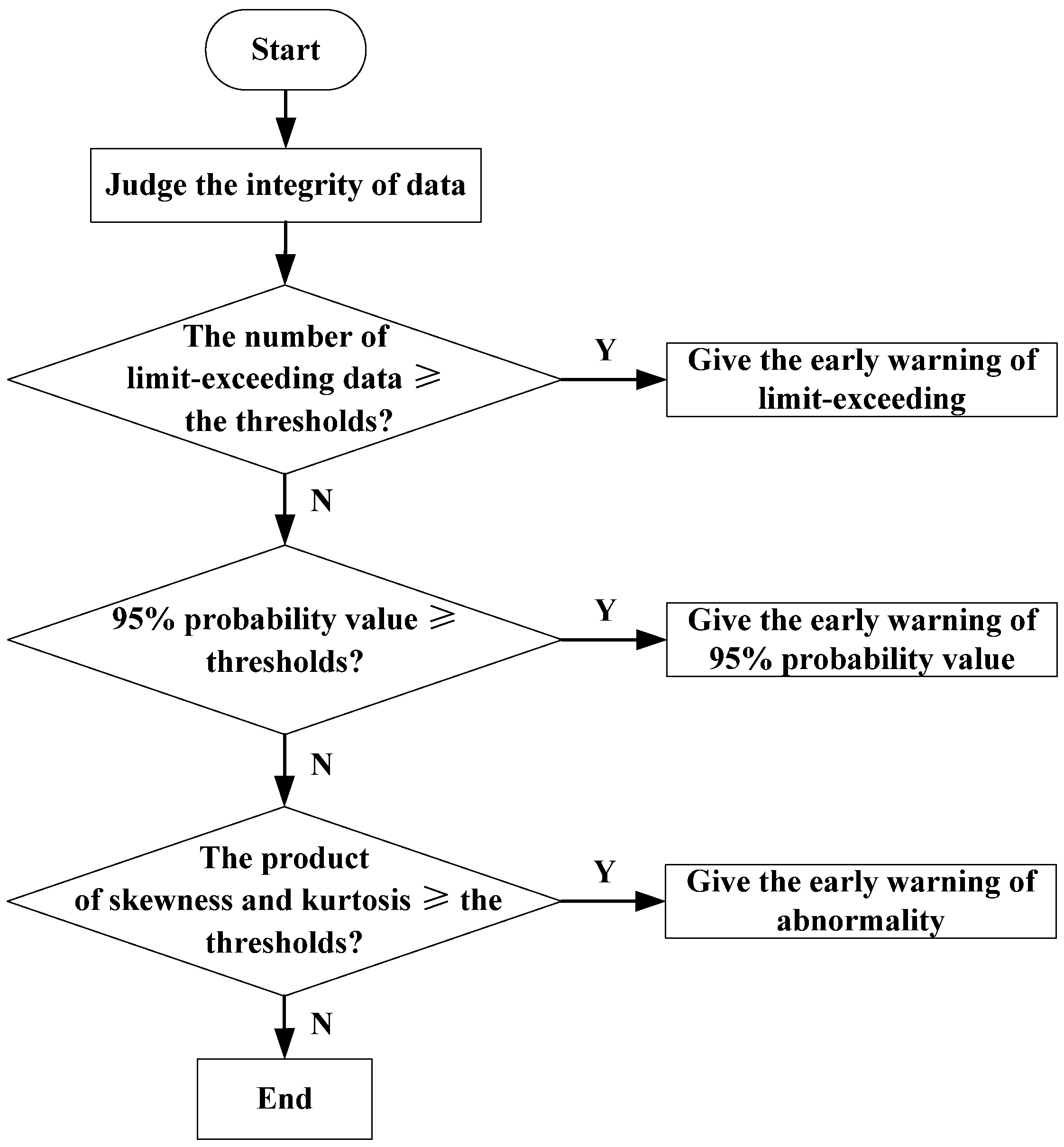
In the process of anomaly detection, the product of the skewness and kurtosis is often compared with the thresholds for Grades 2 or 1 to judge whether the data is abnormal.

As the flowchart shown in Figure 2, the specific early warning standard for anomaly detection is that, if the average and maximum of this product exceed the corresponding thresholds, a Grade 2 early warning should be given; if either the average or maximum exceed the thresholds, a Grade 1 early warning should be given. If neither the average nor the maximum of the product exceed the thresholds, the PQ data are judged to be normal.

Figure 2. Early warning flowchart.

Figure 2. Early warning flowchart.

4. PQ Decision Support Approach

Decision analysis is natural human behavior, and decision support systems have been widely used in many fields to help decision makers solve non-programmed problems [27,28]. In this study, the decision support approach is applied to provide PQ control methods advice, in order to improve PQ. The methods include both qualitative analysis and quantitative analysis. The qualitative analysis provides PQ measures, and the quantitative analysis is designed to specific parameters for improved measures. The application premises of the decision support approach are PQ early warning. The analysis results can either be used on an already-installed device to improve parameter design, or be used to design parameters for a new device.

In developing a decision support system, a knowledge base should first be established to form a preliminary expert system. This paper proposes the PQ decision support base given in Table 1.

Table 1. Power quality (PQ) decision support base.

PQ Type	Qualitative Analysis
Voltage deviation	thyristor voltage regulator (TVR)
Harmonic	power filter (PF)/active power filter (APF)
Flicker	thyristor controlled reactor (TCR)
Unbalance	static capacitor
Sag	dynamic voltage restorer (DVR)

Table 1. Power quality (PQ) decision support base.

PQ Type	Qualitative Analysis
Voltage deviation	thyristor voltage regulator (TVR)
Harmonic	power filter (PF)/active power filter (APF)
Flicker	thyristor controlled reactor (TCR)
Unbalance	static capacitor
Sag	dynamic voltage restorer (DVR)

This table gives a qualitative analysis for PQ problems. In actual applications, decision support also requires quantitative analysis. During the process, parameters designing for PQ control measures (such as thyristor voltage regulator (TVR)) need to be given. When these parameters are designed, the following methods can be used to calculate the specific results. These results are also a part of PQ decision support analysis.

The quantitative analysis for the design of the thyristor voltage regulator (TVR) parameters is as follows: The TVR’s rated capacity S_TVR is:

$$S_{\text{TVR}}=\sqrt{3}{I}_{\text{TVR}}\cdot U_{\text{TVR}}$$

(11)

where U_TVR is the series transformer’s rated voltage, and I_TVR is the rated current:

$$I_{\text{TVR}}=\frac{S_{NL}}{\sqrt{3}{U}_{NL}}$$

(12)

where S_NL is the transmission capacity of the line and U_NL is the rated voltage of the line.

The TVR transformer design includes its iron core, windings, load loss, iron loss, no-load current, and so on. These are computed as:

$$\{\begin{array}{l}D=K\sqrt[4]{S_1}\\ N=\frac{U_{ФN}}{2.22B_m{S}_c\times {10}^{-2}}\\ S=\frac{I_{Ф}}{J}\\ r_{{75}^{\circ }C}=\frac{0.0375L\text{'}}{S}\\ P_0=K_0(G_{Fe})P_c\\ I\%=\sqrt{{(\frac{Q_m+Q_J}{10S})}^2+{(\frac{P_0}{10S})}^2}\%\end{array}$$

(13)

where D is the diameter of the iron core; S₁ is the capacity of each column in the transformer; K is an empirical coefficient; N is the number of windings; S_c is the sectional area of each column; B_m is the magnetic flux density; U_ΦN is the rated phase voltage; S is the sectional area of wire; I_Φ is the phase current; J is the primary density of the current value; r_75oC is the single-phase resistance of aluminum wire; L’ is the cord length; P₀ is the iron loss; K₀ is a technological coefficient of no-load loss; G_Fe is the total weight of iron core; P_c is the unit loss; I% is the no-load current; Q_m is the excitation volt-ampere; and Q_J is the seam volt-ampere.

The other PQ indices can be similarly analyzed. The main design parameters of power filter (PF) are:

$$\{\begin{array}{l}C=\frac{I_{fn}\left(n^2-1\right)}{U_1{w}_s{n}^2\sqrt{n}}\\ L=\frac{U_1\sqrt{n}}{w_s\left(n^2-1\right)I_{fn}}\\ R=\frac{n{w}_{s}L}{Q_{opt}}\end{array}$$

(14)

where I_fn is the n-th harmonic current; n is the harmonic order; U₁ is the fundamental wave voltage; w_s is the angular frequency; and Q_opt is the quality factor.

The electric reactor of the TCR is designed according to:

$$I_N=\frac{Q_{TCR}}{3U_N}$$

(15)

where Q_TCR is the rated capacity of TCR and U_N is the system voltage of TCR. Additionally, the electric reactor design should satisfy thermal stability and dynamic stability requirements.

The main parameters for the static capacitor design are:

$$\{\begin{array}{l}{U}_N=\frac{C_A+{\text{α}}^2{C}_B+\text{α}{C}_C}{C_A+C_B+C_C}\\ C_A+C_B+C_C=C_N{U}_{CN}/(U_N-U_{CN})\end{array}$$

(16)

where U_N is the neutral displacement voltage; C_A, C_B, C_C are three static phase capacitors; α = e^j2π/3; C_N is the neutral point capacitor; and U_CN is the neutral point displacement voltage.

The capacity of the DVR is:

$$S=U_{DVR}\times I_L$$

(17)

where I_L is the rated current of the load; U_DVR is the effective value of the compensating voltage.

Based on the changes of voltage sag, the ratio of transformer can be chosen. In general, its value can be set to be greater than 1.

The energy of DC-side capacitor can be chosen from storage battery, or rectification circuit. The specific parameters can be designed as required.

5. Implementation of the Proposed Approach

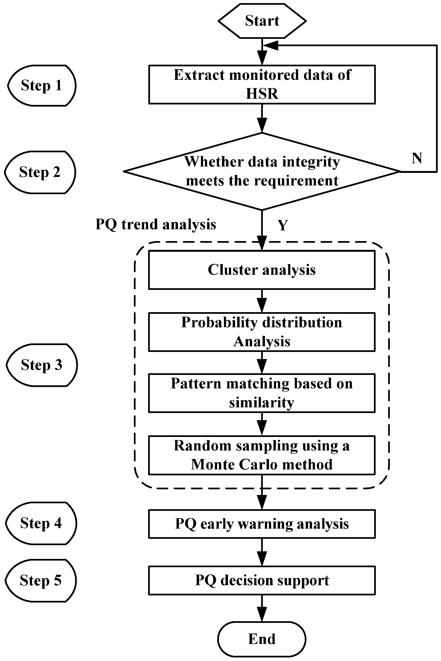
Using the methods described in previous sections, we can conduct PQ trend analysis, early warnings, and decision support. A flowchart of the proposed approach is shown in Figure 3. Its implementation proceeds as follows:

Step 1: Extraction of historical monitored data

Monitoring equipment is used to acquire monitored PQ data and environmental variables about the wind farm.

Step 2: Judge the integrity of the monitored data.

In this step, the number of monitored data is compared against the requirements of data integrity. If the requirement is met, proceed to Step 3; if not, the monitored data should be reselected.

Figure 3. Main flowchart of PQ early warning based on trend analysis.

Figure 3. Main flowchart of PQ early warning based on trend analysis.

Step 3: PQ trend analysis.

(a) Cluster analysis based on DTW distance.

First, the DTW distances of the environmental variables should be computed.

Then, according to experience, the threshold for cluster analysis can be determined, and similar environmental data can be put in the same category.

Finally, using the same classification, the monitored PQ data belonging to the same category can be clustered.

(b) Analyze probability distribution.

Statistical methods are used to compute the probability distribution, and polynomial fitting is used to compute the distribution function of the monitored PQ data and environmental variables.

(c) Pattern matching based on similarity.

Environmental variables for the following day can be obtained from the weather forecast. Then, based on the DTW algorithm, the similarity of the predicted and historical environment variables can be computed. The target value is the minimum of the matching coefficient.

(d) Random Monte Carlo sampling.

Obtain the PQ probability distribution of the minimum value given in step (c). Using Monte Carlo sampling and the dichotomy method, random samples can be generated to analyze the predicted PQ data.

Step 4: PQ early warning analysis

Based on the three-level, four-grade mechanism, an early warning analysis of the PQ trend predicted data can be conducted, and rational early warning prompts can be given.

Step 5: PQ decision support

According to the early warning results, qualitative and quantitative PQ decision support is provided. In this manner, both power suppliers and users can be informed about future anomalous PQ changes, and advised on corresponding countermeasures to reduce relevant losses.

6. Case Studies

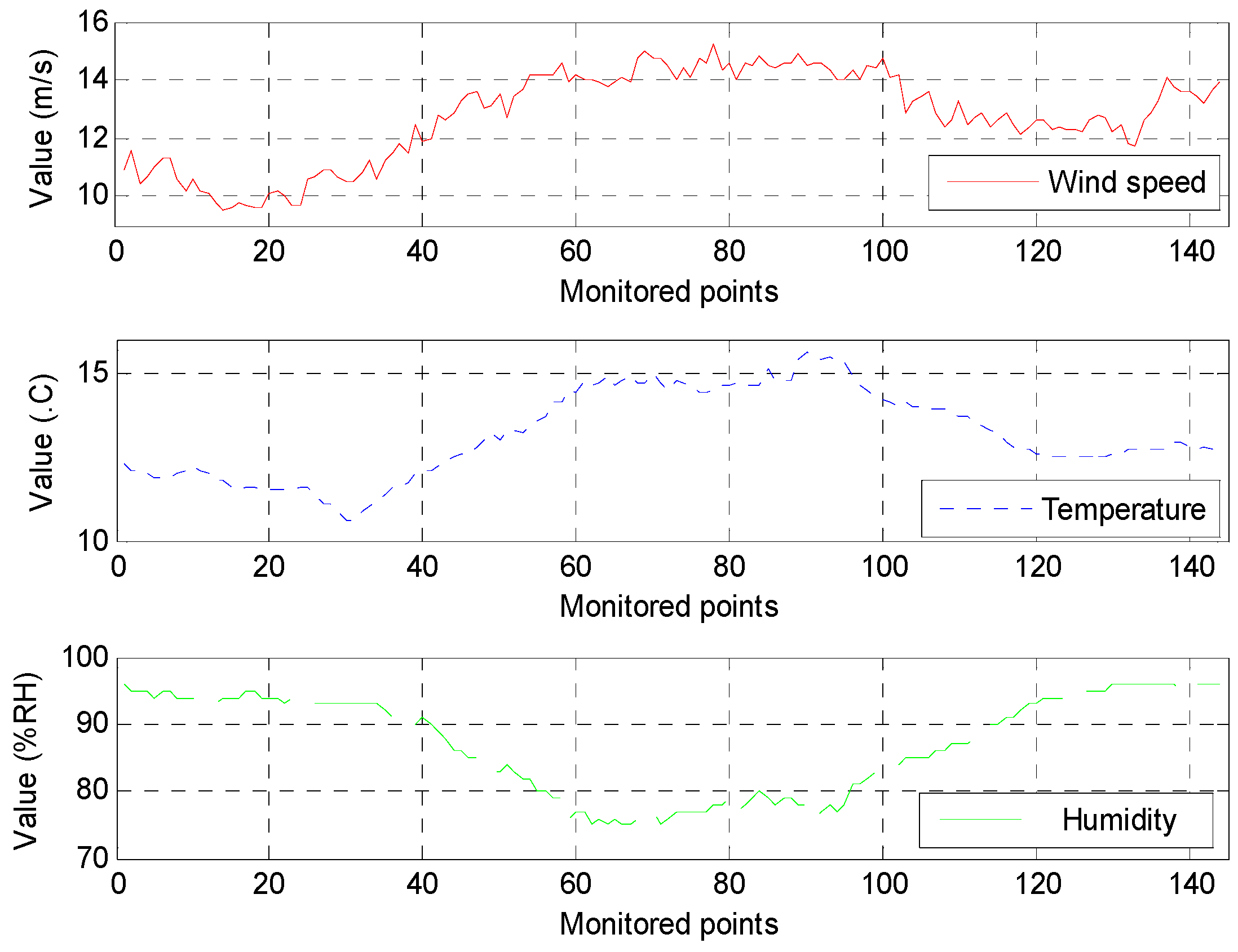
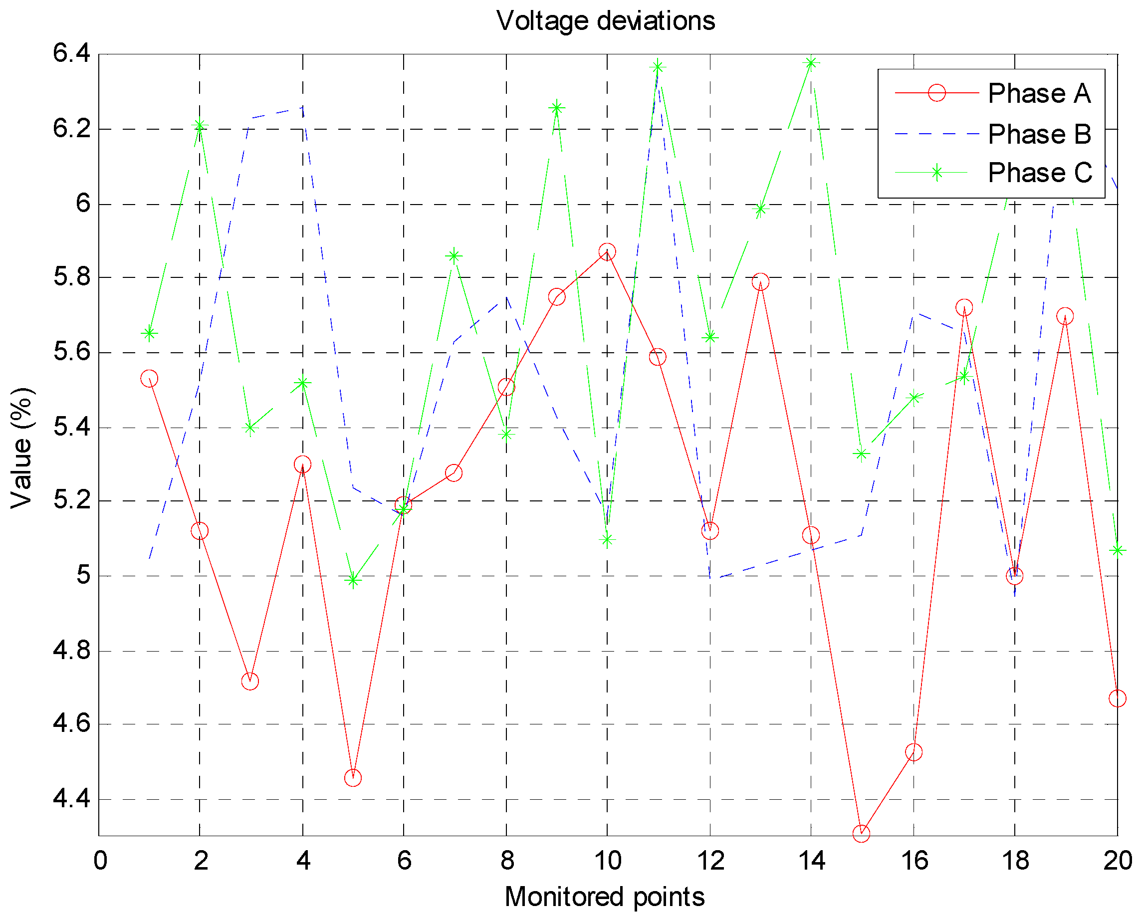
The Jiangsu Power Supply Company in China has established a large-scale PQ monitoring network. The network achieves the real-time monitoring of large PQ disturbances, and performs remote data transmission using a standardized network encapsulation protocol. This provides a good basis for the data sources needed for PQ monitoring, analysis, and control.

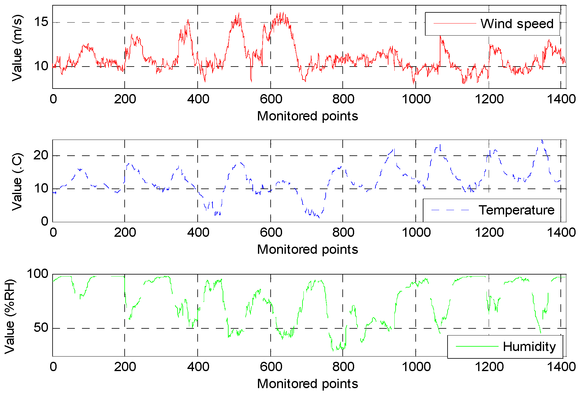
To test the effectiveness of the proposed approach, we consider the example of monitored waveform data from the 220 kV I-bus bar at the Dafeng wind farm of Jiangsu Province, China, from 1–10 April 2014. The wind farm is located in a coastal region, which is rich in wind energy. There are 174 grid-connected wind turbine generators, and the total capacity is 200.25 MW. The waveforms of the environmental variables and voltage deviations over the ten-day period are shown in Figure 4 and Figure 5, respectively.

Figure 4. Data waveforms for environmental variables.

Figure 4. Data waveforms for environmental variables.

Figure 5. Data waveforms for voltage deviations.

Figure 5. Data waveforms for voltage deviations.

6.1. Cluster Analysis Based on DTW Distance

To describe their relative importance, we first compute the weights of different environmental variables. The monitored environmental variables include the wind speed, temperature, and humidity. Using the expert scoring method, the wind speed, temperature, and humidity are assigned weights of 0.85, 0.15, and 0.05, respectively.

Based on these weights and the DTW algorithm, we can analyze the DTW distances between environmental variables for the ten-day experimental period. The results are shown in Table 2.

In this case, after several debugging cycles, we found that the results were improved by setting the threshold for cluster analysis to 15. Based on this threshold and the DTW distances in Table 2, the sample data from the monitored days can be divided into the categories shown in Table 3.

Table 2. Comprehensive Dynamic Time Warping (DTW) distances between environmental variables for the ten-day experimental period.

	1	2	3	4	5	6	7	8	9	10
1	0	8.9202	18.1395	28.4813	36.0505	28.9780	28.1076	17.9547	13.2252	15.1751
2	8.9202	0	10.3344	18.7757	24.4030	26.8658	25.5321	12.0432	11.6296	10.5289
3	18.1395	10.3344	0	16.2891	12.2257	28.4933	31.4876	13.3668	17.9953	16.5128
4	28.4813	18.7757	16.2891	0	15.9106	24.3856	34.3268	21.8502	26.6840	23.7939
5	36.0505	24.4030	12.2257	15.9106	0	40.0936	39.7421	26.0072	38.5885	30.7590
6	28.9780	26.8658	28.4933	24.3856	40.0936	0	28.7244	27.2740	29.0994	27.3337
7	28.1076	25.5321	31.4876	34.3268	39.7421	28.7244	0	23.5939	29.1371	24.2365
8	17.9547	12.0432	13.3668	21.8502	26.0072	27.2740	23.5939	0	9.2964	7.5905
9	13.2252	11.6296	17.9953	26.6840	38.5885	29.0994	29.1371	9.2964	0	10.9283
10	15.1751	10.5289	16.5128	23.7939	30.7590	27.3337	24.2365	7.5905	10.9283	0

Table 2. Comprehensive Dynamic Time Warping (DTW) distances between environmental variables for the ten-day experimental period.

	1	2	3	4	5	6	7	8	9	10
1	0	8.9202	18.1395	28.4813	36.0505	28.9780	28.1076	17.9547	13.2252	15.1751
2	8.9202	0	10.3344	18.7757	24.4030	26.8658	25.5321	12.0432	11.6296	10.5289
3	18.1395	10.3344	0	16.2891	12.2257	28.4933	31.4876	13.3668	17.9953	16.5128
4	28.4813	18.7757	16.2891	0	15.9106	24.3856	34.3268	21.8502	26.6840	23.7939
5	36.0505	24.4030	12.2257	15.9106	0	40.0936	39.7421	26.0072	38.5885	30.7590
6	28.9780	26.8658	28.4933	24.3856	40.0936	0	28.7244	27.2740	29.0994	27.3337
7	28.1076	25.5321	31.4876	34.3268	39.7421	28.7244	0	23.5939	29.1371	24.2365
8	17.9547	12.0432	13.3668	21.8502	26.0072	27.2740	23.5939	0	9.2964	7.5905
9	13.2252	11.6296	17.9953	26.6840	38.5885	29.0994	29.1371	9.2964	0	10.9283
10	15.1751	10.5289	16.5128	23.7939	30.7590	27.3337	24.2365	7.5905	10.9283	0

Table 3. Classification of working conditions.

Type	1	2	3	4	5	6
Day	1, 2	9, 10	3, 8	4, 5	6	7

Table 3. Classification of working conditions.

Type	1	2	3	4	5	6
Day	1, 2	9, 10	3, 8	4, 5	6	7

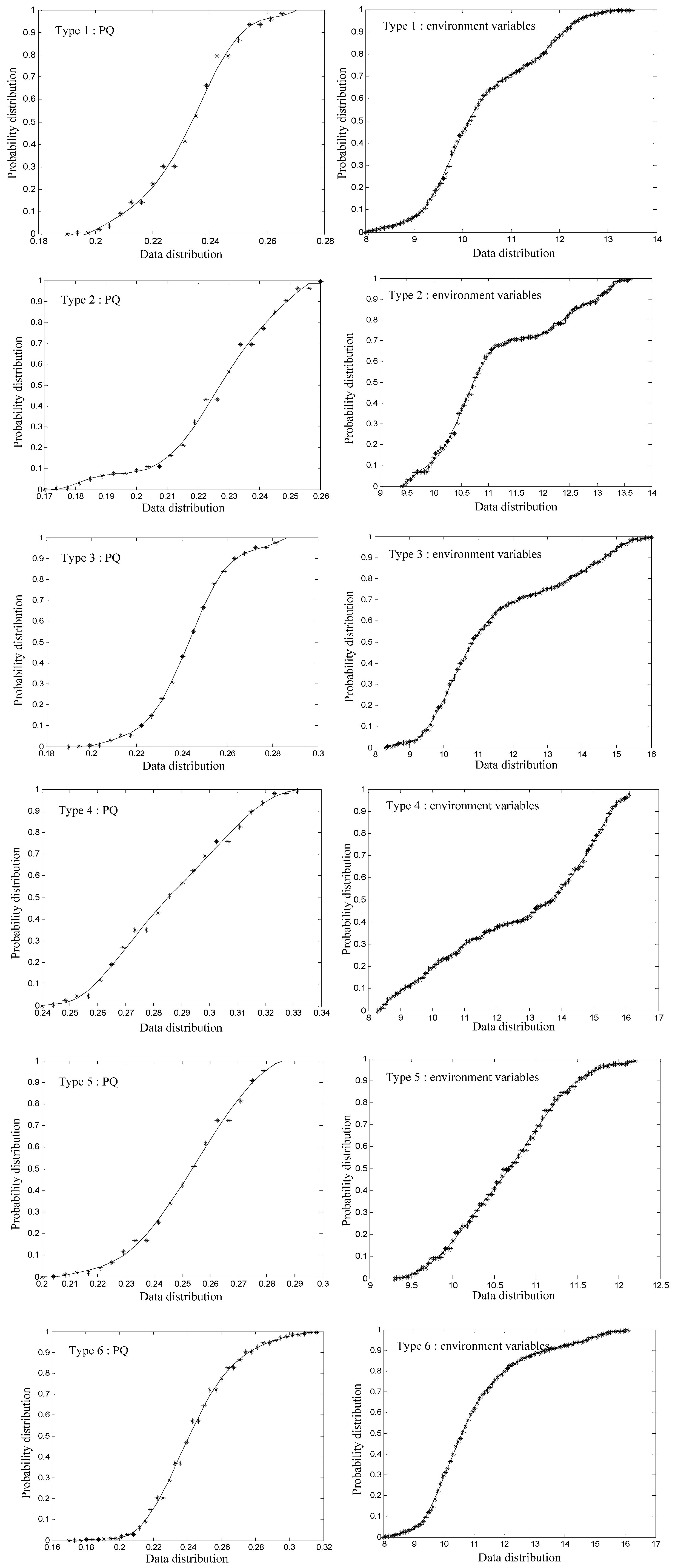
6.2. Probability Distribution of Classified Working Conditions

By classifying historical monitored days, the monitored PQ data and environment variables that belong to the same category can be placed together. Statistical methods allow us to compute the relevant probability distribution graphs. The left-hand side of Figure 6 shows the probability distributions of monitored PQ data in different working conditions. The right-hand side shows the probability distributions of the corresponding environment variables (Figure 6 takes wind speed as an example; the other environment variables are not shown). Finally, we use the polynomial fitting method to compute the specific probability distribution functions.

Based on the above analysis, we can establish the relation between PQ and environment variables. Pattern matching of the environment variables determines the corresponding PQ probability distributions, enabling the PQ trend analysis to be conducted.

Figure 6. Probability distribution functions of classified working conditions.

Figure 6. Probability distribution functions of classified working conditions.

6.3. Pattern Matching Based on Similarity

According to the weather diagnostics, environment variables for the next day can be obtained. Waveforms of the predicted environment variables are shown in Figure 7.

Figure 7. Waveforms of predicted next-day environment variables.

Figure 7. Waveforms of predicted next-day environment variables.

The DTW distances between the above data and six types of sample data can then be computed, from which we obtain the similarity results given in Table 4.

Table 4. Similarity between test data and database samples.

Type	1	2	3	4	5	6
Test Data	67.52%	60.74%	60.19%	52.21%	52.01%	58.11%

Table 4. Similarity between test data and database samples.

Type	1	2	3	4	5	6
Test Data	67.52%	60.74%	60.19%	52.21%	52.01%	58.11%

In Table 4, Type 5 represents different working conditions. According to the results of cluster analysis, the data can be divided into six types. The actual debugging shows that the number of classification is appropriate. At this time, the difference among the types is relatively big, and the similarity among the same type is relatively high. Each type can reflect one corresponding working condition. The corresponding PQ probability distributions of different types are as follows (take phase A for example):

Type 1: F(x) = 10¹⁸ × (1.8303 × x⁹ − 0.8247 × x⁸ + 0.1647 × x⁷ − 0.0191 × x⁶ + 0.0014 × x⁵ − 0.0001 × x⁴);

Type 2: F(x) = 10¹⁸ × (2.2317 × x⁹ − 0.9793 × x⁸ + 0.1904 × x⁷ − 0.0215 × x⁶ + 0.0016 × x⁵ − 0.0001 × x⁴);

Type 3: F(x) = 10¹⁸ × (1.1706 × x⁹ − 0.5229 × x⁸ + 0.1034 × x⁷ − 0.0119 × x⁶ + 0.0009 × x⁵);

Type 4: F(x) = 10¹⁸ × (3.6834 × x⁹ − 1.6375 × x⁸ + 0.3216 × x⁷ − 0.0366 × x⁶ + 0.0027 × x⁵ − 0.0001 × x⁴);

Type 5: F(x) = 10¹⁸ × (2.4598 × x⁹ − 1.0995 × x⁸ + 0.2176 × x⁷ − 0.0250 × x⁶ + 0.0018 × x⁵ − 0.0001 × x⁴);

Type 6: F(x) = 10¹⁸ × (2.7872 × x⁹ − 1.2993 × x⁸ + 0.2684 × x⁷ − 0.0322 × x⁶ + 0.0025 × x⁵ − 0.0001 × x⁴);

From Table 4, we can see that the Type 1 working condition provides the best match with the test data. Thus, we extract the PQ probability distribution for this type, and proceed to the next step.

6.4. Producing Predicted PQ Trend Data

Based on the Monte Carlo and dichotomy methods, we generate random samples for the Type 1 PQ data probability distribution. The results are the predicted PQ trend data, and their waveforms are shown in Figure 8.

Error values can be computed by comparing the predicted data with the actual data. We conducted a normality test on the error values, and found that p = 0.1690 > 0.05. Therefore, the error values can be considered to obey a normal distribution. The average and variance of the error values was computed as 0.020750 and 0.000230, respectively (ε ~ N (0.020750, 0.000230)).

Setting the confidence level α to 0.9997, the value of the risk function VaR^* is 0.03127. If we define the excessive loss and lack of value loss functions as 0.3 ε and 0.3 ε², respectively, the predicted interval is [y − 0.104233, y + 0.322850] (risk value is 0.0003).

Upon testing, all predicted data were found to be within the above interval, meaning the risk of the error value is under control. Therefore, the results of our PQ trend analysis are reliable and meaningful.

Figure 8. PQ trend predicted data.

Figure 8. PQ trend predicted data.

6.5. PQ Early Warning

Based on the predicted PQ trend data and our three-level, four-grade early warning mechanism, we examined the performance of our PQ early warning approach for voltage deviations. The analysis results are as follows.

(1) Predicted PQ trend data do not exceed the thresholds for limit-exceedance, and therefore do not prompt a limit-exceeding warning.

(2) The 95% probability value does not exceed the corresponding thresholds, and no 95% probability value warning is given.

(3) According to actual needs, the thresholds for the maximum and average of the product of the skewness and kurtosis can be set to 100 and 30, respectively. The maximum and average of the predicted data are 136.280177 and 19.430737, respectively. Therefore, a Grade 1 abnormal warning can be given.

6.6. PQ Decision Support

Our PQ trend analysis and early warning results show that future voltage deviations may cause anomalous changes in power supply, and it is therefore necessary to provide decision support. On the grounds of our PQ decision support base, the qualitative measure for reducing the voltage deviation concerns the TVR. Using Equations (11)–(13), the main parameters for the TVR are designed, and the results are given in Table 5. These are parts of quantitative analysis, and can be a reference for practical application.

Table 5. Quantitative analysis for main design parameters.

Parameters	ITVR	STVR	D	N10kV	N600V	S10kV	S600V	r75°C	P0	I%
Values	115.5 A	120 kW	145 mm	1770	106	3.31 mm2	38.5 mm2	7.46 Ω	367 W	7.3 A

Table 5. Quantitative analysis for main design parameters.

Parameters	ITVR	STVR	D	N10kV	N600V	S10kV	S600V	r75°C	P0	I%
Values	115.5 A	120 kW	145 mm	1770	106	3.31 mm2	38.5 mm2	7.46 Ω	367 W	7.3 A

7. Conclusions

This paper has presented a new PQ trend analysis approach, the results of which can be used to provide early warnings about anomalous PQ changes. We also described a decision support method that provides reference information to improve PQ for both power suppliers and users. The increasingly open electricity market and focus on PQ means that the results of this study can be used to develop a software system to supplement and perfect the existing PQ monitoring platform. Such a system could also provide technical support to prevent accidents and effectively improve the reliability and economy of the power grid.