1. Introduction
The Organic Rankine Cycle (ORC) is an effective method to recover energy from the low grade heat sources [
1]. The ORCs are Rankine cycles that use an organic fluid, characterized by a high molecular mass and a low evaporation point. The low-temperature heat is converted into work, and, then, it can be converted into electricity [
2]. The first prototype of an ORC was developed in 1961 by the engineers Tabor and Bronicki.
The advantages of ORC are varied. The organic substance used is usually characterized by a low boiling point, a low latent heat of evaporation and high density. These properties are preferable to increase the inlet mass flow rate of the expander. Then the specific heat of evaporation of the organic fluid is considered lower than that of water; this is the main reason for which the organic fluids are used in place of water for the recovery of heat from sources in the medium-low temperature range. Another important factor that has contributed to the diffusion of the ORC, is the possibility of adapting the same system for different heat sources with minor changes—the components used, in fact, can be derived from air conditioning ones, which have already reached the full technological maturity stage. The favorable performance of ORCs in energy recovery, if adopted by industrial facilities, could ease electricity demand, concomitantly decreasing fossil fuel consumption, and increasing consumers’ overall energy efficiency. ORC, at present, are available in the range up to 100 kW, and only a few solutions are suitable and commercially available for lower outputs. Our target is to fill this gap by studying and realizing a small (2–5 kW) ORC energy recovery system and in the present study we propose its adoption for vehicular applications [
3,
4,
5].
2. The ORC Recovery Energy System
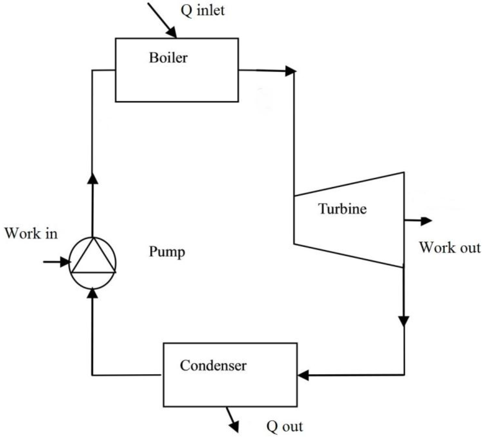
The Organic Rankine Cycle (ORC) is similar to a conventional steam power plant, with the exception of the working fluid, which in this case is an organic fluid with suitable chemical-physical proprieties. The fluid selection depends on the temperatures of both the thermal source and thermal sink. Heavy hydrocarbons, HCFC, and other synthetic fluids still under evaluation can be used.
Figure 1 shows an example of an ORC plant. It is a closed cycle plant, constituted by a pump, two heat exchangers and an expander.
Depending on the system possibilities, additional intermediate heat recoveries can be considered. The Organic working fluid is compressed by a booster pump and fed to the heat recovery vapor generator (HRVG), where it is evaporated and becomes superheated vapor. The superheated vapor enters a turbine and expands to a low pressure to generate the power output. Afterwards, the turbine exhaust is condensed to a liquid in the condenser by rejecting heat to the environment. In the ORC system, the condenser is a very important component which can influence the overall system performance regarding the heat sink of thermodynamic cycle.
Figure 1.
Layout of an ORC system.
Figure 1.
Layout of an ORC system.
It can be noticed that the ORC technology has been extensively studied in recent years, and applications are known for:
In the proposed ORC plant, the heat source can be the exhaust gases of a vehicle thermal engine. The ORC operates as a “bottoming energy recovery system”. Part of this “waste heat” energy amount is directly converted in mechanical work through the turbine, and supplied, by an electric generator/inverter, to a possible final user. The remaining amount of energy at low temperature at the condenser, can be used, if necessary, for heating the vehicle.
3. ORC Thermodynamic Analysis
3.1. Simulation
A thermodynamic cycle has been designed for electrical energy production in the 2–5 kW range with the following technological limitations: a single stage radial turbine is chosen as the expander; the condensation temperature limit should not be less than 300 K, the overall dimension of all components has to be limited, for vehicular applications. As thermal source the exhaust gas of a typical 2.0 L Diesel engine, or from a small size turbine engine, has been considered. Thermodynamic gas conditions are summarized in
Table 1. In all cycles proposed, the same heat source is used; in this way it is possible to evaluate the “quasi-optimal” system configuration.
Table 1.
Thermal source main data.
Table 1.
Thermal source main data.
| Data | Value |
|---|
| Mass flow rate (kg/s): | 0.15 |
| Exhaust temperature (K): | 845.15 |
| Pressure (kPa): | 202.6 |
| Average Composition (per cent by volume): | CO = 0.041; |
| CO2 = 2.74; |
| O2 = 17.14; |
| CxHy ≤ 0.03 |
Prior to its use “on board”, the water needed for condensation, may be the same as the vehicle’s cooling circuit (both car and boat), so, the cooling water, in the simulation (cold source), comes from a tank and it is introduced into the condenser by a pump. In the considered application, the vehicle cooling secondary circuit can be used. Consequently, its mass flow rate is limited to 1 kg/s (
Table 2).
Table 2.
Inlet cooling water main data.
Table 2.
Inlet cooling water main data.
| Data | R134a | R245fa |
|---|
| Mass flow rate (kg/s) | 1 | 0.7 |
| Temperature (K) | 288.15 | 288.15 |
| Pressure (kPa) | 150 | 150 |
In this paper the thermodynamic properties and the performance of the cycles with the organic fluids R245fa and R134a are compared.
R134a: 1,1,1,2-Tetrafluoroethane, R-134a, Florasol 134a, or HFC-134a, is a haloalkane refrigerant, it has the formula CH2FCF3 and a boiling point of 246.85 K at atmospheric pressure. 1,1,1,2-Tetrafluoroethane is an inert gas used primarily as a “high-temperature” refrigerant for domestic refrigeration and automobile air conditioners.
R245fa: HFC-245fa is also known as pentafluoropropane and by its chemical name 1,1,1,3,3-pentafluoropropane. Unlike the CFC and HCFC blowing agents formerly used for this purpose, it has no ozone depletion potential and is nearly non-toxic.
3.2. Process Simulation with CAMEL-ProTM
To analyze the ORC plant performance a steady state simulation of the plant has been performed with the CAMEL-Pro
TM Process Simulator [
6,
7]. The computer code for the modular simulation of energy conversion processes was developed as part of the research conducted by the “CIRCUS” group (International Centre for Research and Scientific Computing University Department of Mechanics and Aeronautics) at University of Roma “Sapienza”. The code developed (in C++ and C#), called CAMELPro
TM (an acronym for Modular CAlculation for ELements) is characterized by being designed from the outset as an Object Oriented program; and it is composed by two parts: a central body that only perform the common operations in any simulator (reading input, graphical interaction with the user, assembly of a power plant, presentation of the results), and a library of “elements” (expandable) containing independents structures. The elements can be represented by an object or component, that are modularly interfaced with other components.
4. The Plant Layout and Simulation Results
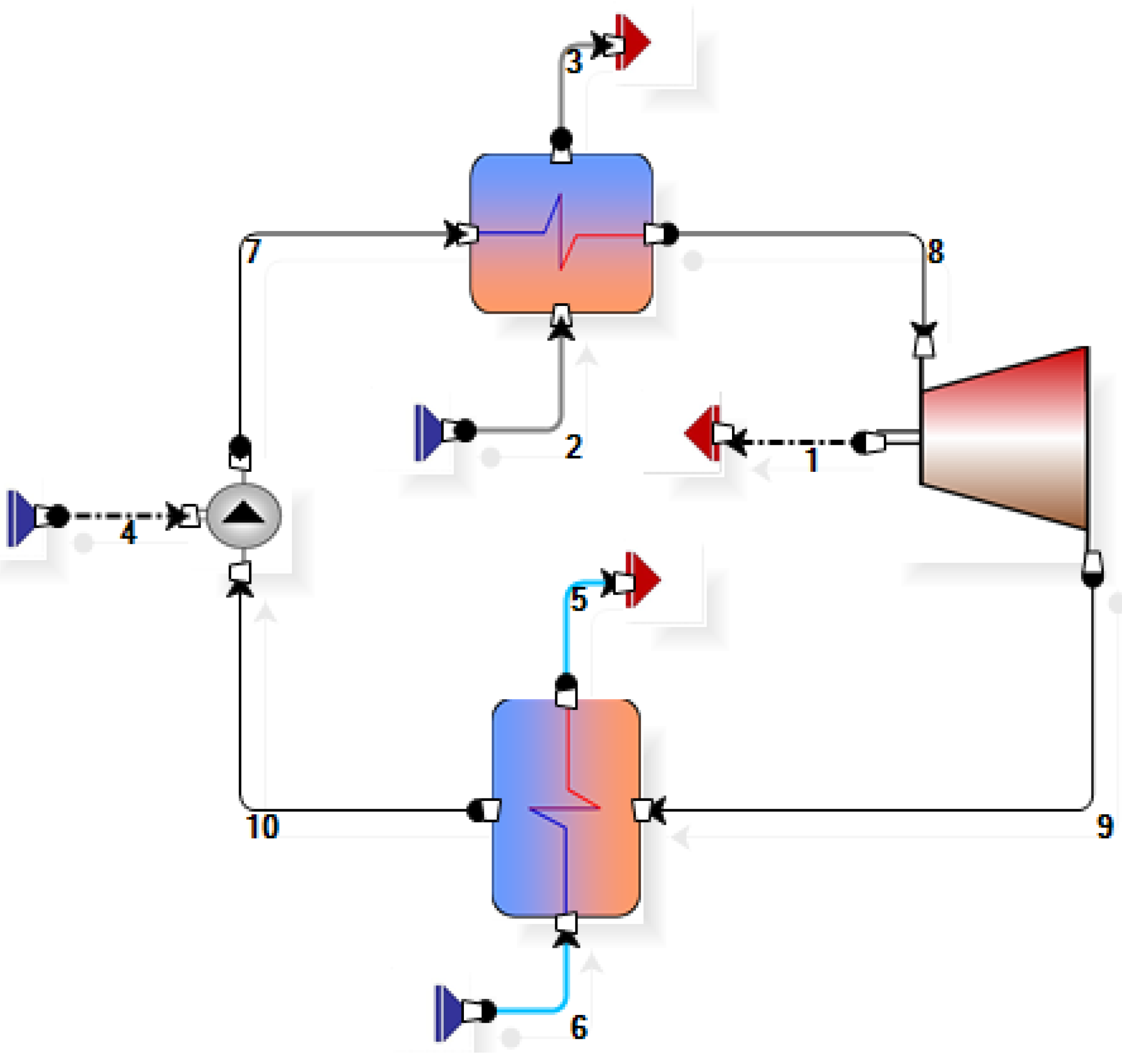
The layouts studied in this paper with the organic fluids R134a and R245fa are shown in
Figure 2. The variables fixed are:
Figure 2.
Layout with R134a and R245fa.
Figure 2.
Layout with R134a and R245fa.
All other thermodynamic variables were considered independent. The criterion for modeling the thermodynamic cycles is to obtain the required power using the lowest mass flow rate of organic fluid. The simulations results of the cycles are presented below (
Table 3 and
Table 4).
In
Figure 2, the different phases of simulated thermodynamic cycle are presented:
Also designated are:
exhaust gas inlet (2),
exhaust gas exit (3),
cooling water inlet (6),
cooling water outlet (5),
mechanical power absorbed by the pump (4),
power output produced (1).
Table 3.
Simulation results the of R134a case.
Table 3.
Simulation results the of R134a case.
| Data | Unit | Value |
|---|
| R134a mass flow rate | (kg/s) | 0.38 |
| R134a boiler inlet temperature (7) | (K) | 307.48 |
| R134a boiler outlet temperature (8) | (K) | 334.20 |
| R134a condenser inlet temperature (9) | (K) | 315.29 |
| R134a condenser outlet temperature (10) | (K) | 306.80 |
| R134a boiler inlet pressure (7) | (kPa) | 1670 |
| R134a boiler outlet pressure (8) | (kPa) | 1500 |
| R134a condenser inlet pressure (9) | (kPa) | 950 |
| R134a condenser outlet pressure (10) | (kPa) | 874 |
| Outlet gas temperature (3) | (K) | 402.16 |
| Outlet cooling water temperature (5) | (K) | 304.48 |
| Power output (1) | (kW) | 3.526 |
| Power absorbed by pump (4) | (kW) | 0.302 |
Table 4.
Simulation results of the R245fa case.
Table 4.
Simulation results of the R245fa case.
| Data | Unit | Value |
|---|
| R245fa mass flow rate | (kg/s) | 0.35 |
| R245fa boiler inlet temperature (7) | (K) | 315.21 |
| R245fa boiler outlet temperature (8) | (K) | 345 |
| R245fa condenser inlet temperature (9) | (K) | 326.23 |
| R245fa condenser outlet temperature (10) | (K) | 315 |
| R245fa boiler inlet pressure (7) | (kPa) | 680 |
| R245fa boiler outlet pressure (8) | (kPa) | 612 |
| R245fa condenser inlet pressure (9) | (kPa) | 300 |
| R245fa condenser outlet pressure (10) | (kPa) | 270 |
| Outlet gas temperature (3) | (K) | 403.59 |
| Outlet cooling water temperature (5) | (K) | 311 |
| Power output (1) | (kW) | 4.463 |
| Power absorbed by pump (4) | (kW) | 0.124 |
The advantages provided by ORC cycles are more significant than the respective water cycle, both in terms of power produced and efficiency. The results are reported in
Table 5. It can be noticed that, especially the R245fa cycle, is very close to the Carnot efficiency, while for the water cycle, efficiency is much lower. In addition, the net power produced in the R245fa cycle is 104% greater and in the R134a cycle it is 77% greater than in the water/steam cycle.
Table 5.
Characteristics of thermodynamic cycle.
Table 5.
Characteristics of thermodynamic cycle.
| Data | R134a | R245fa | Water cycle |
|---|
| Net power product (kW) | 3.224 | 4.329 | 2.084 |
| Evaporator (kW) | 71.53 | 71.31 | 72.77 |
| Condenser (kW) | 68.23 | 66.88 | 70.68 |
| Efficiency | 4.5% | 6% | 2.9% |
| Carnot efficiency | 8.2% | 8.7% | 9% |
Simulation is needed to identify the operational conditions of the various components, especially the condenser, the subject of this study. In addition, only the results of the simulation were reported, without any comment as, the code has already been widely validated in numerous papers, that have demonstrated its validity, reliability and precision and in addition, because our focus is on how to design and realize the components.
Finally, it can be underlined how after the two simulations, R134a organic fluid has been chosen as operating fluid. The reasons lies in the fact that the fluid is “not so” expensive, readily available, and its technology is “completely” mature. The R245fa fluid has the best performance but its reliability is yet to be improved. Since the purpose of the research is to develop an operational and reliable prototype, the choice necessarily fell on the R134a option.
5. Thermodynamic Model of the Condenser
The first step was the definition of the design constraints. In the ORC plants, the condenser occupies more available space than the others components (expander and boiler). Since the aim is to create a system, that can be installed “on board” a car or in a small boat, the condenser design procedure has always to consider this limitation as a design target. To maximize the heat exchange and reduce the component size, copper elements for were used exchange surfaces, which allows an excellent thermal performance, and presents compatibility with the use of refrigerants. Furthermore, the counter flow configuration has been chosen.
5.1. Selection of Tube-Fin Heat Exchanger
To obtain a compact heat exchanger a configuration, characterized by a high ratio between the heat exchange surface and the occupied volume has to be chosen. The area density, β, is the ratio of heat transfer area to its volume [
8]. There are some additional advantages for small volume as follows: low weight, easier transport, better temperature control. A heat exchanger tube and fins type has been adopted. This exchanger is characterized by a high density of exchange surface, reduction of load losses, and it avoids technological and fouling problems that are present in the compact type ones (sometimes, improperly, used as condensers) such as radiator and plate heat exchangers [
9,
10].
5.2. “LMTD Method” and “Heat Exchanger Effectiveness Method”
LMTD is defined as follows:
Here Δ
T1 and Δ
T2 are the temperature drops between two fluids at each end of a counter flow exchanger. For a counter flow exchanger, in our case, Δ
Th,i and Δ
Th,o indicate the inlet and outlet temperatures of condensing fluid, and the inlet and outlet temperatures of cooling fluid, respectively. The heat transfer equation is given by:
where “
F” is
LMTD correction factor. It is equal to unity for a true counter flow exchanger. When the temperature of one fluid is constant (as in a phase-change condition) the factor
F is equal to 1, as in our case [
11]. The exchange surface is evaluated in this way:
Kays and London [
12] have presented “effectiveness ratios” for various heat-exchanger arrangements and in case of condensation too; in this case “effectiveness” can be expressed by the following simple equation:
where a dimensionless property known as number of transfer units (
NTU) is:
In this study, both methods have been considered and used. The LMTD method has been used to find the required area of thermal exchange through an iterative procedure, while the effectiveness method has been used only to evaluate the maximum possible heat transfer and component efficiency.
5.3. Heat Transfer Coefficient
The overall heat transfer, given by combined conduction and convection, is frequently expressed in terms of an overall heat-transfer coefficient “
U”, for the cylinder geometry:
The terms “
Ai” and “
Ao” represent the inside and outside areas of the inner tube. To decrease the number of unknowns of the problem, the calculation of heat transfer coefficient “
U” is only limited to the inner area “
Ai”, and the term “
Ai/
Ao” is replaced by the equation:
5.4. Mono-Phase Heat Transfer and Pressure Drop Correlations
A traditional expression for the calculation of heat transfer, in fully developed turbulent flow in smooth tubes, has been recommended by Dittus and Boelter [
13], linked to Reynolds Number and Prandtl Number:
Nusselt Number (
Nu) is defined as the ratio of the convective heat transfer coefficient (
h) to the pure molecular thermal conductance (
k/
dh). The above equations offer simplicity in computation, but uncertainties on the order of ±25% are not uncommon, as described in the studies of Allen and Eckert [
14]. Then the convective coefficient is evaluated by Nusselt Number as (inside and outside):
In this paper, the pressure drop equation, proposed by Thomas Fanning was used, whit the Fanning friction factor “
f” proposed by Taitel and Dukler [
15]:
“Le” is the equivalent length of the pipe, “ρ” is the density of the gas inside tube, “um” is the fluid velocity in the pipe and “di” is the internal pipe diameter.
5.5. Two-Phase Heat Transfer and Pressure Drop Correlations
For our R134a study, the proposed equation is the result of experimental tests under very close conditions to ours. It is proposed by Balciar
et al. [
16]:
The experimental parameters and operating conditions for this equation are the following:
condensation of R134a in smooth horizontal tubes,
tube inner diameter of 8 mm,
tube length of 2.5 m,
the mass flux between 200 and 700 kg/s,
the number of data point of the study is 280 [
17].
The all liquid equivalent Reynolds number is determined by:
The two-phase density and the Lockhart and Martinelli parameter is determined by the formula:
Also the Froude number is expressed as:
For the R245fa study, the equation derived from a correction of Dobson-Chato method [
18], after the tests with the two-phase fluid R245fa (mixtures for the quality in the range of
to
, in tubes with 7 mm inner diameter). Several tests has been made, and the formula has been presented by Al-Hajri in 2012 [
19], and has a degree of accuracy estimated in ±20%, between the predicted value and the estimated value. The heat transfer coefficient is defined as the liquid heat transfer coefficient, multiplied by the inverse of the Martinelli parameter (
Xtt):
For the organic fluids R134a and R245fa a two-phase friction pressure drop equation is proposed by Kedzierski and Goncalves [
20]:
The specific volume of the two-phase fluid “
v” was obtained from a linear quality weighted sum of the vapor and liquid volumes, at the outlet or inlet of the segment “
Le”. The total mass velocity “
G”, and the properties for the two-phase friction factor “
fN” are evaluated at a linearly averaged refrigerant temperature. The new two-phase friction factor is:
The friction factor is based on the all liquid Reynolds number.
and the two-phase number
. The NIST measured pressure drop data is predicted with an average residual of 10.8% for all pressure drop ranges and refrigerants [
21].
6. Preliminary Design of the Condenser
6.1. Tube and Fins Geometry
The heat exchange coil is composed of “
Nt” tubes, as follows:
“Ns” is the number of tubes where the mass to condense is distributed, and they are arranged in parallel mode,
“Nr” is the number of turns of tubes.
Then the total number of tubes, “
Nt”, is given by
and the total heat transfer area is
. Tubes of thermal exchange are characterized by an inner diameter “
di”, a length “
L1”, and an thickness “
Th”. For the study of heat exchange on finned side, the Briggs and Young correlation [
22] has been used, that is based on regression analysis:
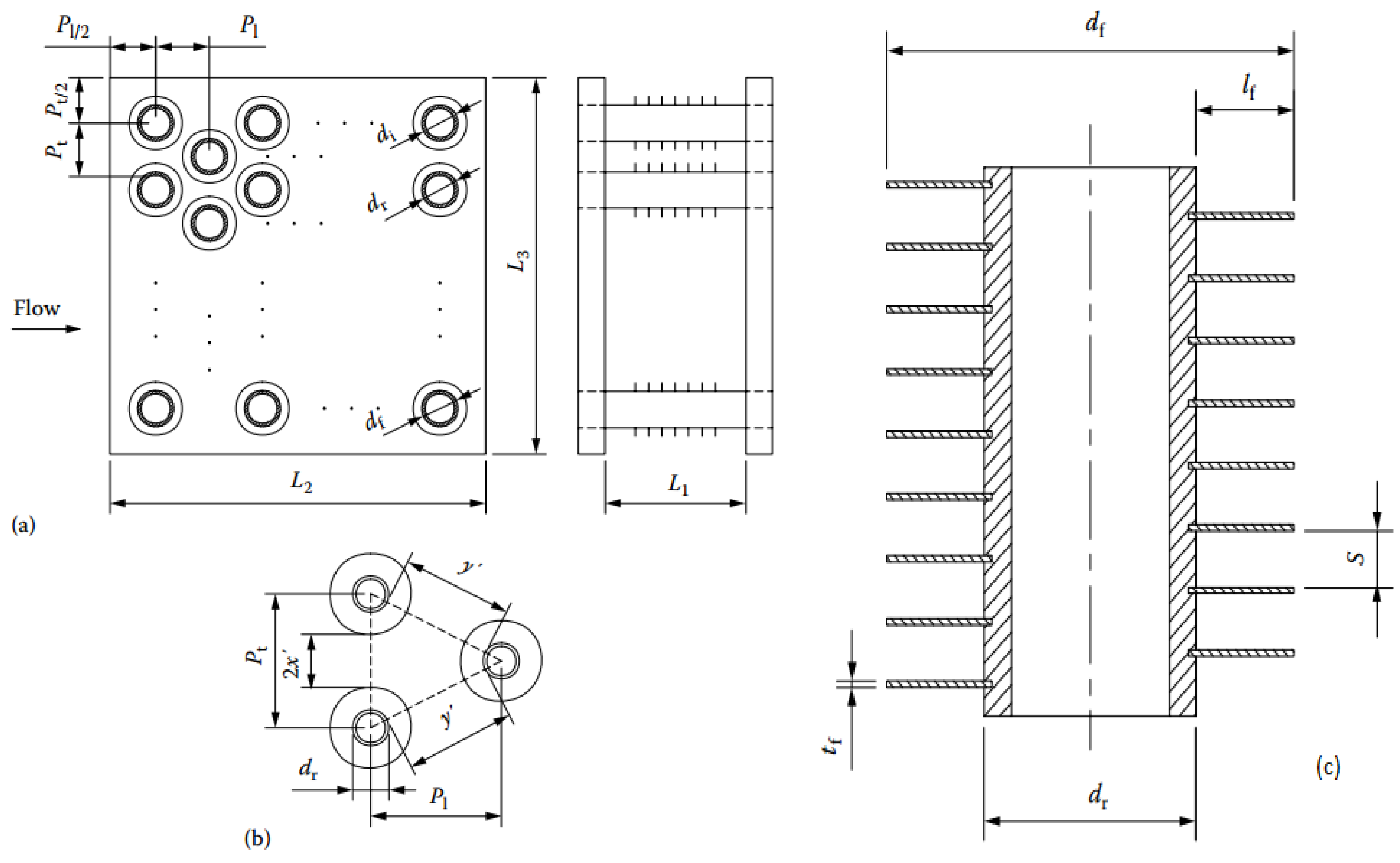
With a standard deviation of 5.1%. The basic core geometry of the exchanger is with a staggered arrangement tubes and is shown in
Figure 3.
Figure 3.
Tube fin details. Individually finned tube staggered arrangment. (a) Geometry; (b) unit cell and (c) tube fin details.
Figure 3.
Tube fin details. Individually finned tube staggered arrangment. (a) Geometry; (b) unit cell and (c) tube fin details.
The total external heat transfer area consists of the area associated with the exposed tubes (primary area) and fins (secondary area). The primary area, “
Ap”, is the tube surface minus the area blocked by the fins. It is given by:
where “
tf” is the fin thickness, “
Nf” is the number of fins per unit length. Furthemore the area of the side plates is added to the heat exchange one. The fin surface area, “
Af”, is given by:
The total heat transfer area Ao is equal to .
6.2. The Problem Approach and the Iterative Calculation
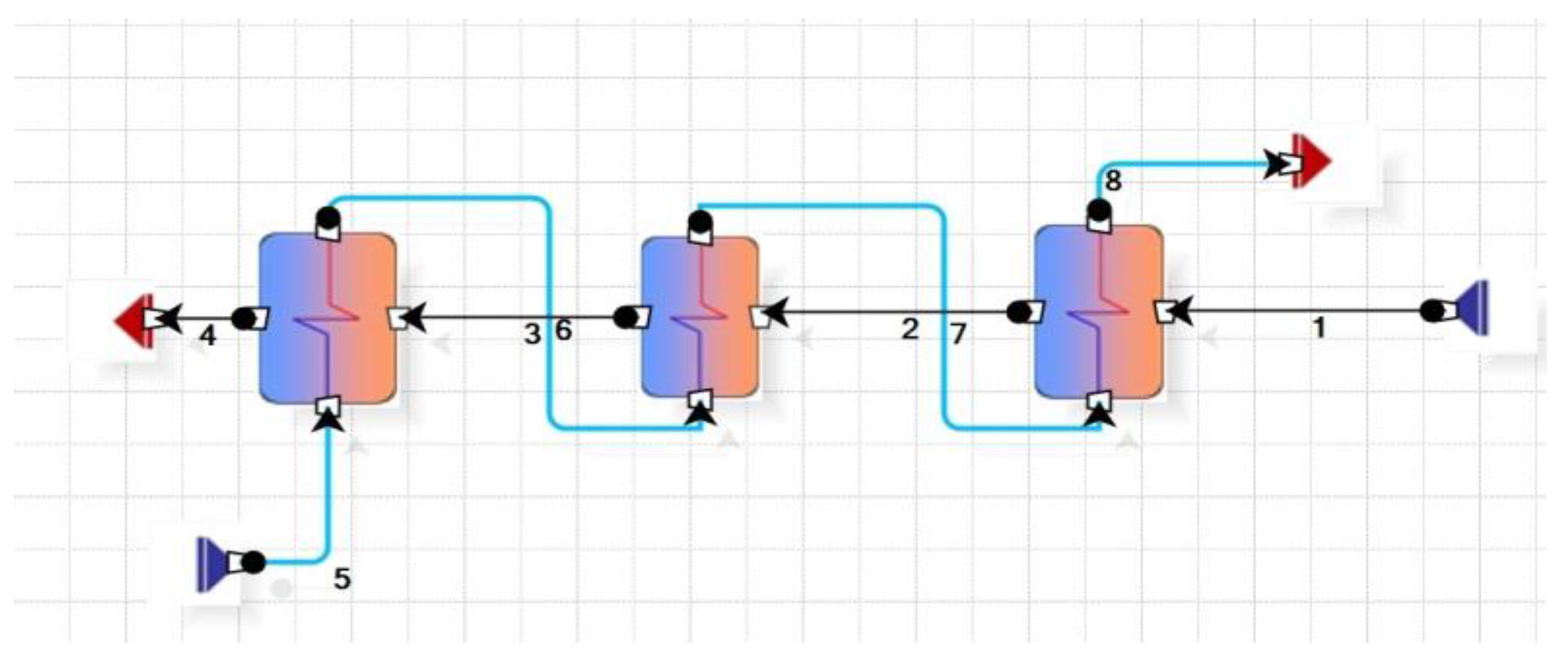
The design of the condenser has been carried out by dividing the process into three consecutive thermodynamic steps (
Figure 4): “Superheated” phase, the “Condensation” phase, and “Sub cooling” phase.
Figure 4.
Separated condenser system using CAMEL-Pro software.
Figure 4.
Separated condenser system using CAMEL-Pro software.
The iterative method consists of several steps, in this way:
The thermodynamic data of three phases have been calculated using the software CAMEL-Pro;
In the same software the temperature drop and thermal power of exchange have been detected;
A starting geometry of study is defined, in terms of tubes numbers “Ns” and “Nr”, their internal diameter, and characteristics of fins;
The hydraulic diameters and the velocity of fluids are calculated, so the values of the convective coefficients of heat exchange and then the global heat exchange coefficient “U”;
The necessary area of heat exchange “A” is calculated, then the component size and its efficiency;
Pressure drops are calculated in the individual phases, which correspond to a new inlet and outlet condensation temperatures;
The problem is set again to get the smallest values of the area “A”, and reduce the overall dimensions of the component.
This iterative procedure has been performed for all the working fluids, in first step with water, then the organic fluid R134a and finally with R245fa fluid. Besides the advantage already mentioned, the organic fluids allow one to obtain a compact size condenser with high heat exchange efficiency. Here, the values of last iteration have been reported and presented.
7. Condenser Design Results for the R134a System
As previously described (see
Section 4), in this research an ORC plant operating with the working fluid R134a has been chosen. The advantages of this choice can be summarized as follows:
Low price of the fluid;
Technology already widely studied and well-established, and with verified formulas for condensation studies;
Efficient and economic turbine for the expansion already present on the market.
All this notwithstanding that the fluid R134a does not have the highest efficiency values, both for the heat exchange or the production of energy. The geometric characteristics found in last iteration are reported in
Table 6, where the number of parallel pipes “
Ns” and number of turns “
Nr”, then the tubes total number “
Nt” have been identified.
Table 6.
Geometric characteristics of R134a component.
Table 6.
Geometric characteristics of R134a component.
| Characteristics | Value | Unit |
|---|
| Inner tube diameter | 6 | mm |
| Tube thickness | 1 | mm |
| Fins distance | 2 | mm |
| Fins height | 3 | mm |
| Fins thickness | 0.3 | nm |
| Tube distance “Pt” | 17 | mm |
| Tube distance “Pl” | 17 | mm |
| Tubes number “Ns” | 15 | - |
| Tubes number “Nr” | 17 | - |
| Total tubes number | 255 | - |
To analyze adequately the condensation phase, the heat transfer process has been divided into 10 sectors, each one characterized by the equal exchanged thermal power “Q
i”, to better distribute the steam quality from the liquid phase to the vapor phase [
15,
16]. In
Table 7,
Table 8 and
Table 9 the results of our assumptions are reported.
Table 7.
Main dimensions of R134a component.
Table 7.
Main dimensions of R134a component.
| Dimensions | Value | Unit |
|---|
| Component length “L1” | 320 | mm |
| Component width “L2” | 265 | mm |
| Component height “L3” | 300 | mm |
Table 8.
Exchanged thermal power.
Table 8.
Exchanged thermal power.
| Thermal power | Value | Unit |
|---|
| Q “Sub-cooling” | 232.8349 | W |
| Q “Condensing” | 66222.436 | W |
| Q “Superheated” | 1774.1024 | W |
| Q “Total” | 68229.374 | W |
Table 9.
Area of heat exchange.
Table 9.
Area of heat exchange.
| Area | Value | Unit |
|---|
| Area “Sub-cooling” | 0.005947 | m2 |
| Area “Condensing” | 1.362625 | m2 |
| Area “Superheated” | 0.098094 | m2 |
| Area “Total” | 1.466666 | m2 |
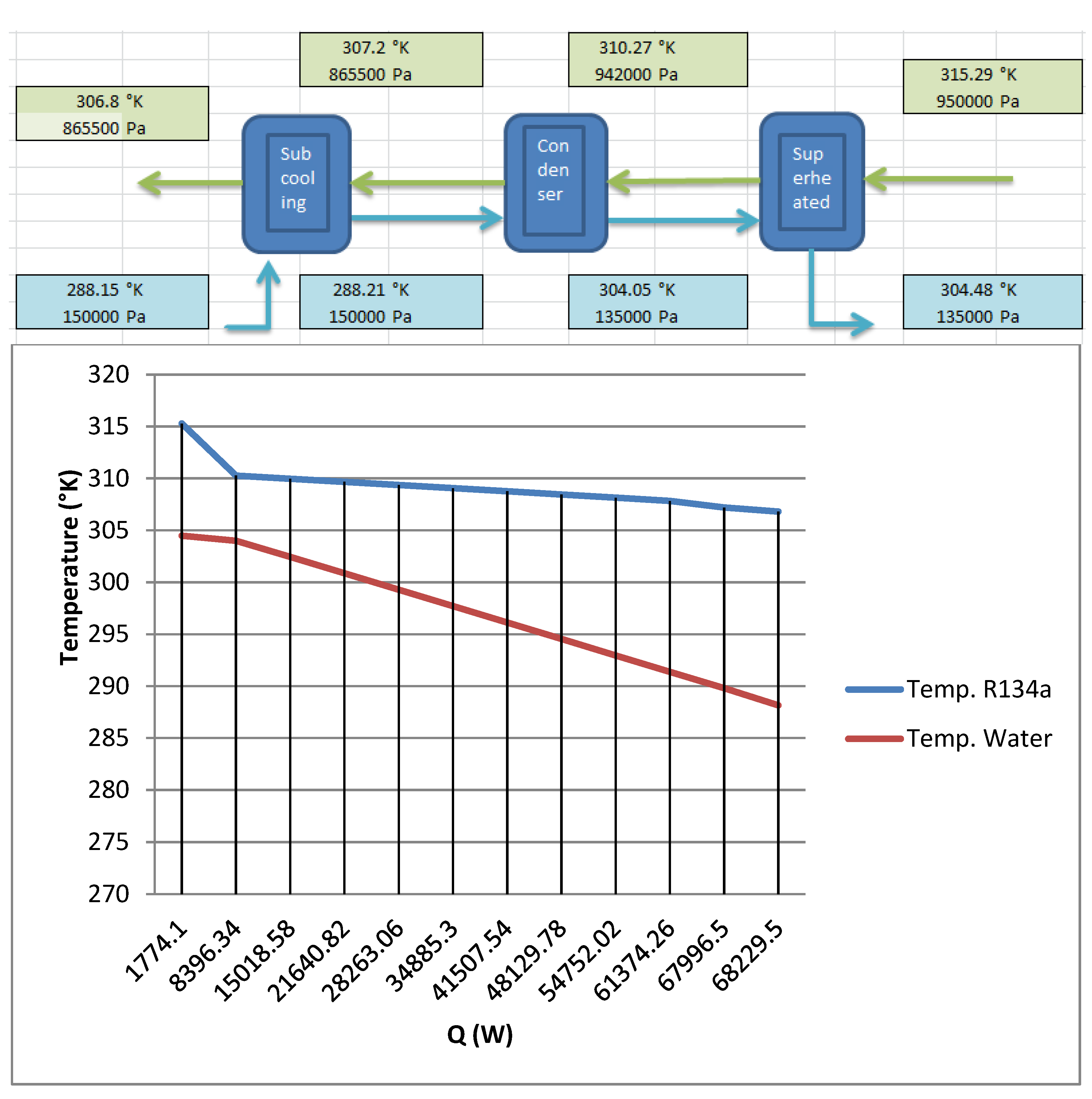
In
Figure 5 the thermal scheme of condensation process, where the values of pressure and temperature are indicated in each thermodynamics zone, for the R134a fluid and the cooling water, are reported. Also the temperature diagram of the fluids during the transfer of heat (Q) is shown.
Figure 5.
R134a thermal scheme.
Figure 5.
R134a thermal scheme.
The overall value of the heat transfer coefficient is:
The total pressure drop is the sum of the pressure drop in each phase:
This represents a loss of 8.86% respect to the inlet pressure. The inner available area of the tubes for the thermal exchange is:
The “effectiveness” of the element is 70%.
7.1. Condenser Design
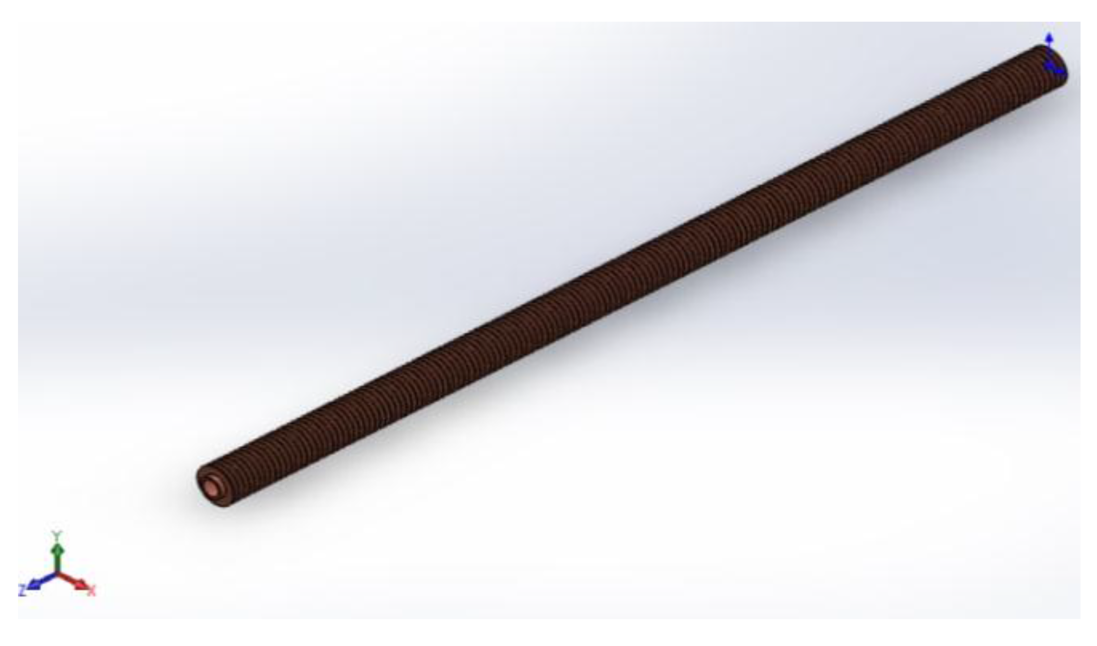
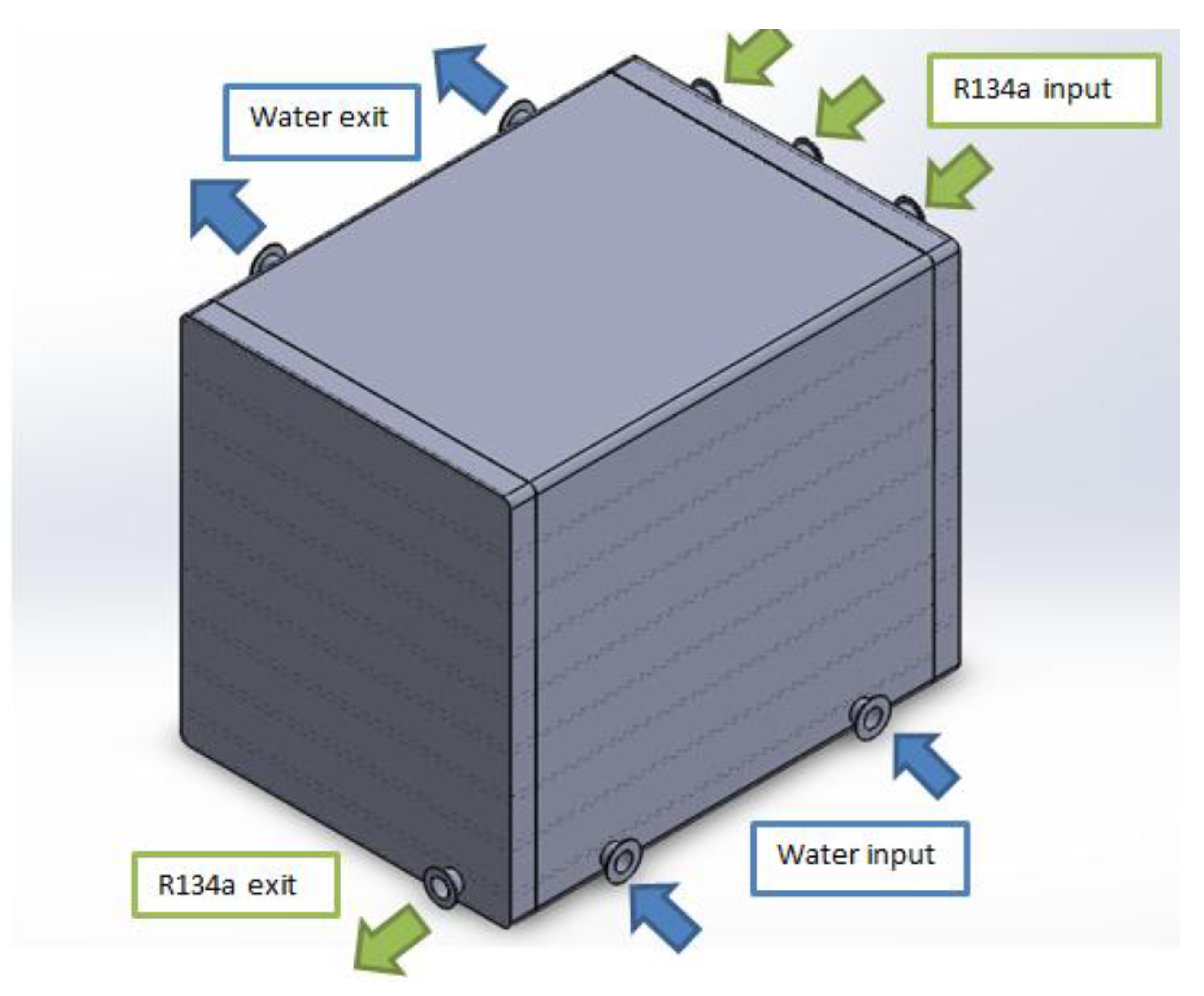
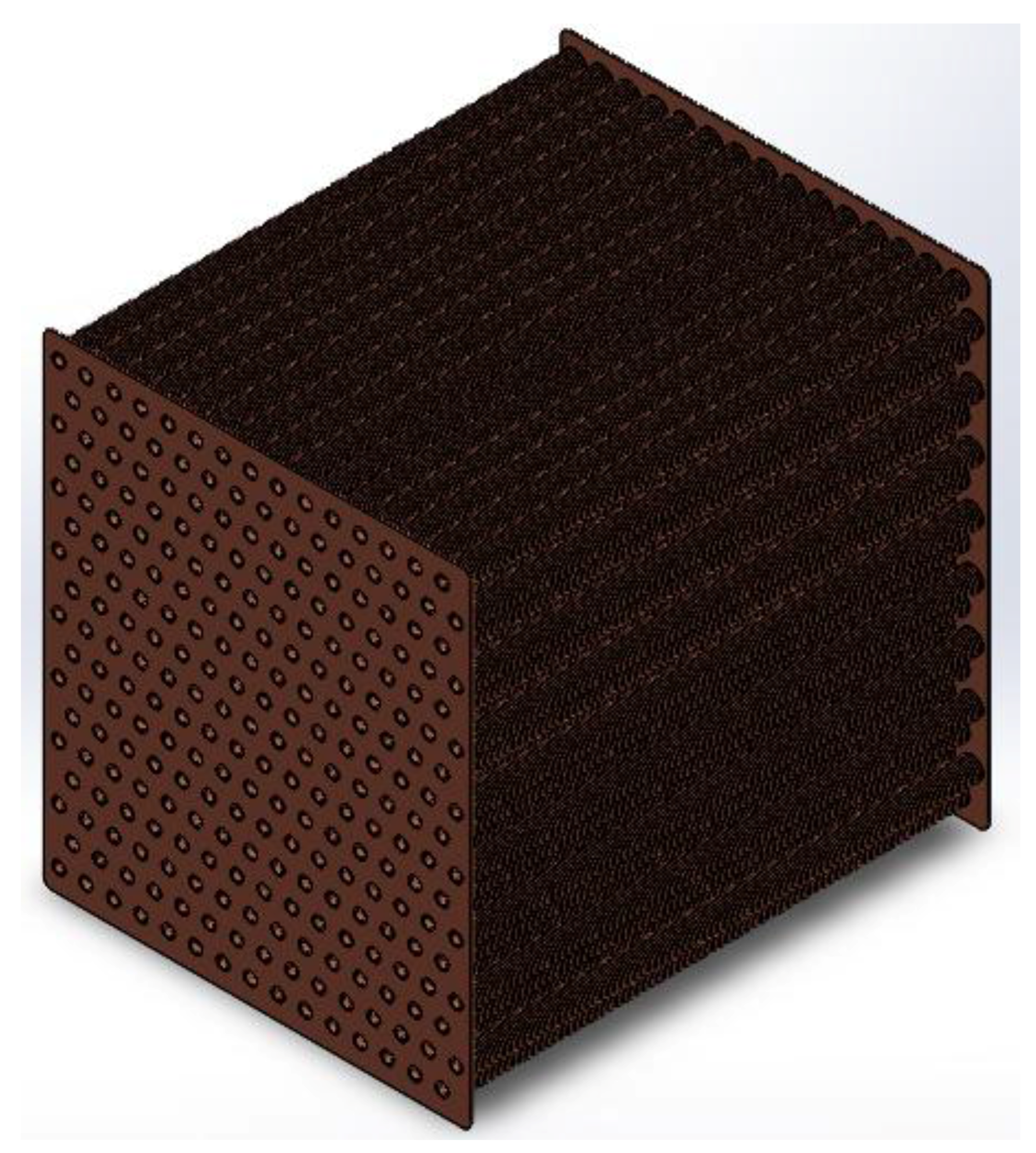
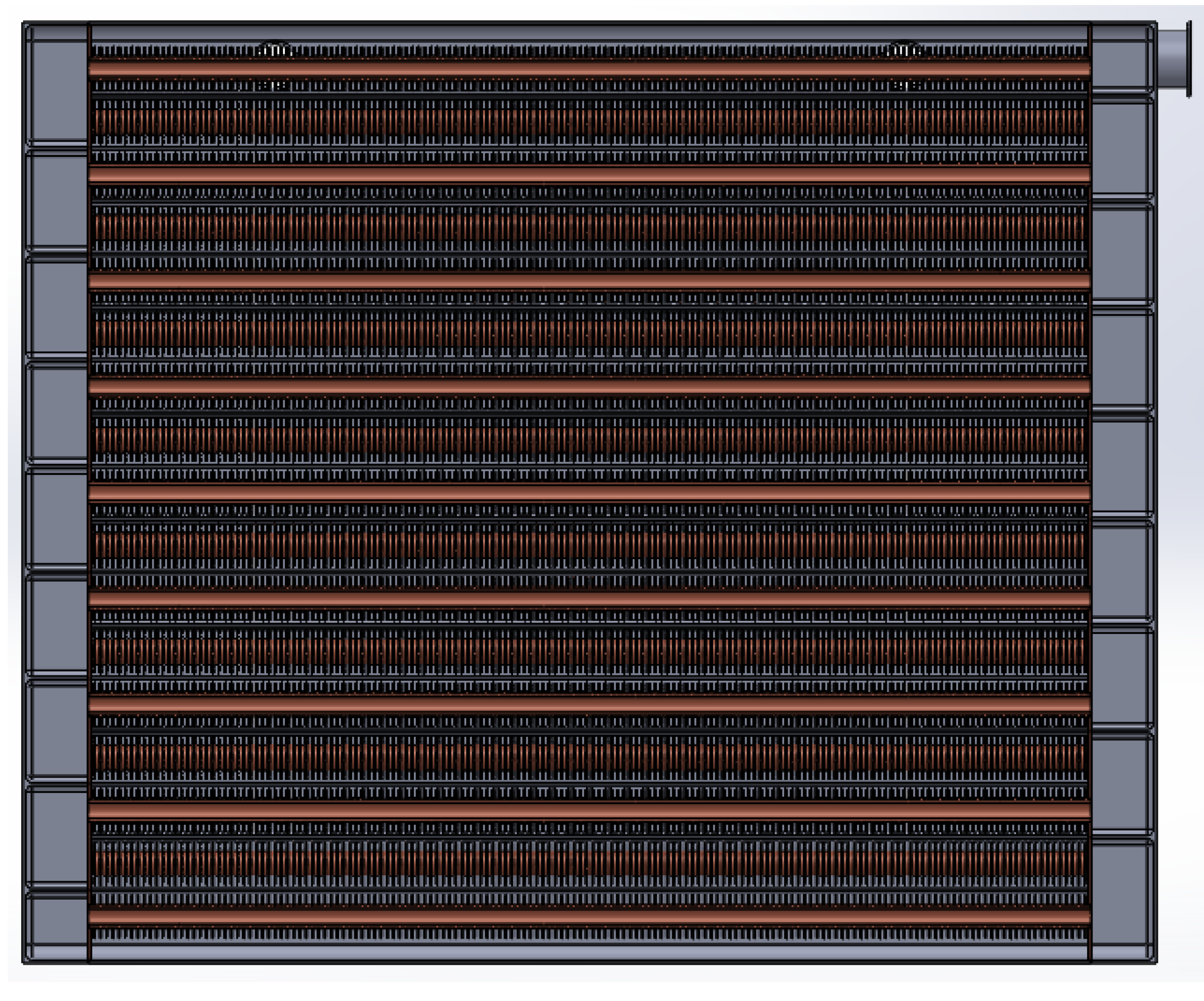
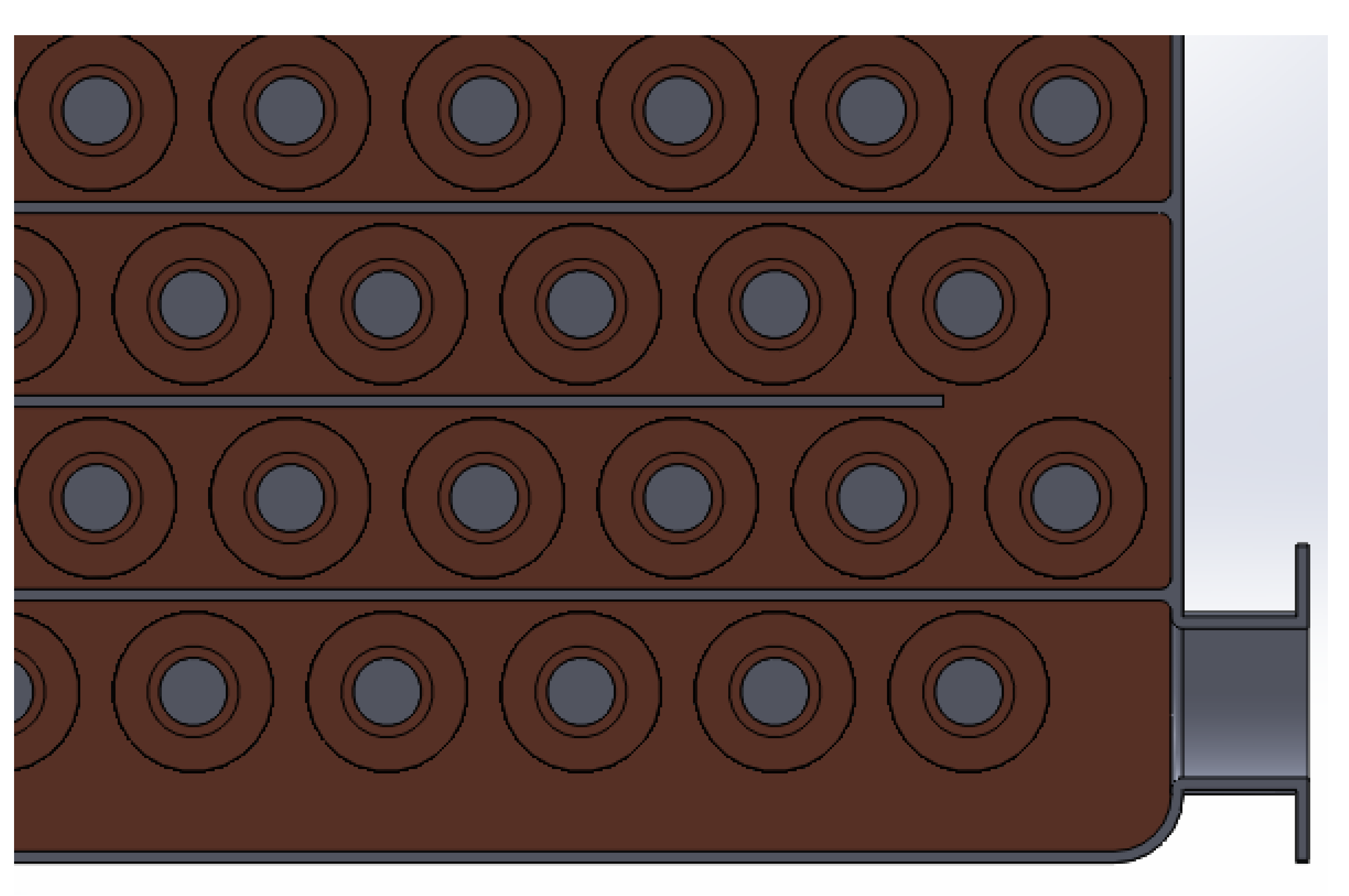
In this section the 3D modeling software SolidWorks® (Dassault Systèmes SolidWorks Corp., Waltham, MA, USA) has been used. The software allows one to create both the 3D model and the dimensional drawings of the parts, to characterize the elements in each part. Then all single mechanical parts of the condenser have been assembled. The elements realized are: the model of the finned tube for the heat exchange, the shell equipped with baffles to guide the cooling water, and two side bulkheads. The next step is the component assembly, where the correct design of all parts and the correct mounting, without interference, have been verified.
The most important part of the condenser is, definitely, the pipe in which the fluid R134a moves. The condenser is composed of 255 tubes as shown in
Figure 6. The parts are assembled to obtain the configuration of
Figure 7, where the fluid inlet and outlet ports are shown. The component provides the R134a inlet ports in the upper zone and outlet ports in the bottom of opposite bulkhead side, while the cooling water enters at the bottom and exits in the upper zone of the shell. This allows one to exploit the thermal effect, during the water heating, and the gravitational effect for the condensate collection, during the transition phase. All the pipes are monted on two grids as shown in
Figure 8. The sectional view of the complete assembly has been represented for clarity in
Figure 9. Finally, in
Figure 10 the details of the R134a inlet port zone are presented.
In the lateral positions there are the two bulkheads made of stainless steel. The function of these parts is to give continuity to the motion of the fluid R134a, during condensation, inside the pipes. The condensing organic fluid inverts its motion in the bulkheads cavity, then its outlet flux, from the parallel tubes (“Ns” indicates the number of tubes), is introduced into the next group of parallel pipes. All the sections of passage for fluids are designed to respect the following velocity limits:
Figure 6.
3D model of the heat exchange tube.
Figure 6.
3D model of the heat exchange tube.
Figure 7.
Scheme of inlet/outlet ports of the condenser.
Figure 7.
Scheme of inlet/outlet ports of the condenser.
Figure 8.
Assembly of the tube-fins parts with the plates, isometric view.
Figure 8.
Assembly of the tube-fins parts with the plates, isometric view.
Figure 9.
Sectional view of the complete assembly, front view.
Figure 9.
Sectional view of the complete assembly, front view.
Figure 10.
Section view of the inlet cooling water zone, side view.
Figure 10.
Section view of the inlet cooling water zone, side view.
All the sections of passage for fluids are designed to respect the following velocity limits:
Maximum cooling water speed is 5 m/s,
Maximum speed of R134a liquid phase is 5 m/s,
Maximum speed of R134a vapor phase is 30 m/s.
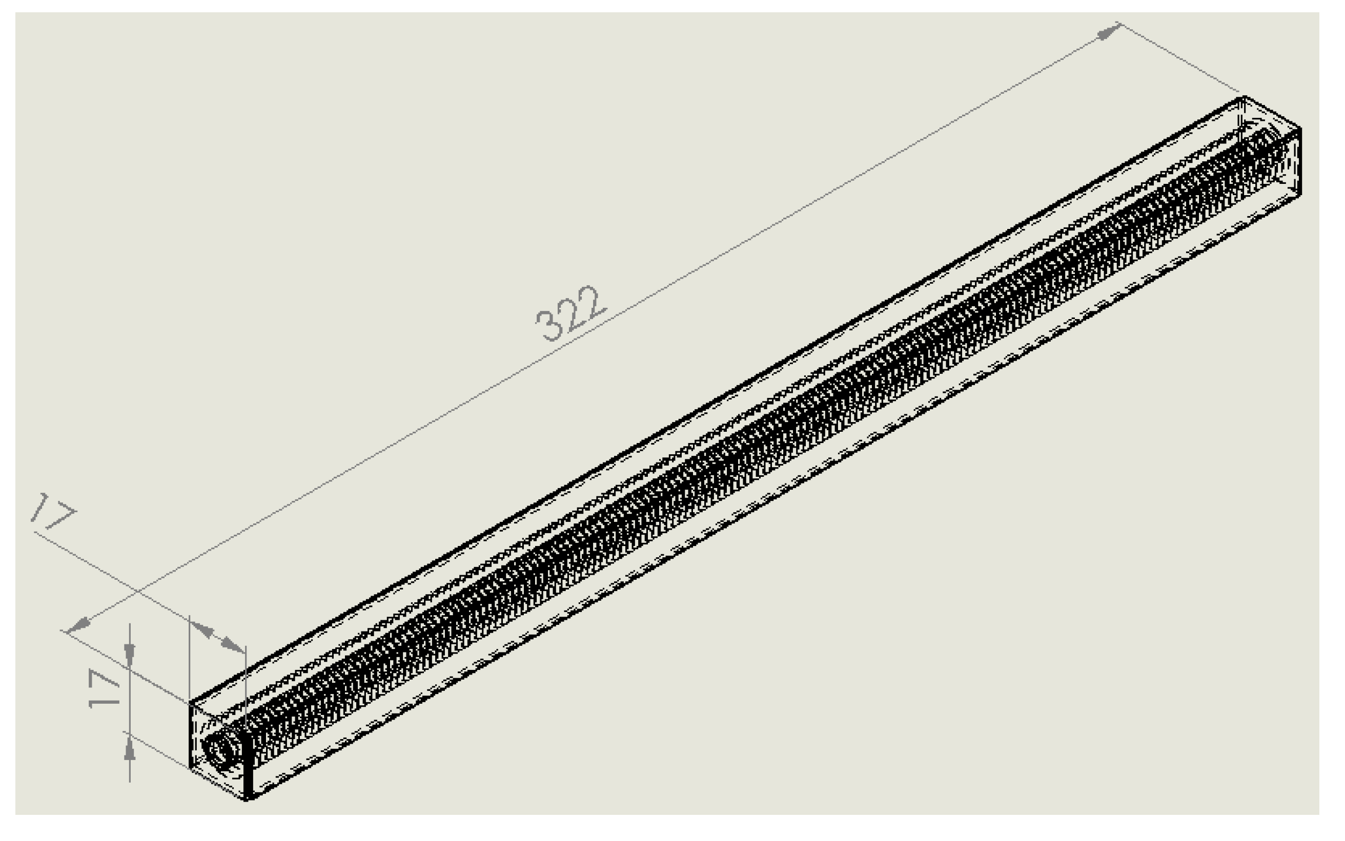
7.2. Superheated Zone CFD Analysis
In the simulation a single pipe has been used; it is inserted in the volume of fluid, between the separator baffles of shell (17 mm), and between the parallel exchange pipes (17 mm) and the two housing plates (
Figure 11). The inlet mass flow rate of cooling water is transversely introduced and exits in the opposite surface, while the R134a (superheated state) passes into the tube. The vapor flow rate is considered as equally distributed in the pipes, and then, for the single heat exchange tube is equal to 0.0253 Kg/s (
Table 10).
Figure 11.
Dimensioned assembly drawing of the CFD study model.
Figure 11.
Dimensioned assembly drawing of the CFD study model.
The mesh of calculation is characterized by:
913,568 elements,
Result resolution of initial mesh level 5,
Heat conduction in solid is set on,
Gravitational effect is set on.
The “Result resolution level of initial mesh” governs the number of Basic Mesh cells and the default procedure of mesh refining, in the model narrow channels. A higher level produces more fine cells, but it will take greater CPU time and require more computer memory. An intermediate level, to optimize this situation, has been selected.
Table 10.
Simulation boundary conditions.
Table 10.
Simulation boundary conditions.
| Boundary conditions | Inlet R134a | Outlet R134a | Inlet water | Outlet water |
|---|
| Pressure (Pa) | 950,000 | - | 147,000 | - |
| Temperature (°K) | 315.29 | - | 304.05 | - |
| Mass flow rate (kg/s) | - | 0.0253 | - | 1 |
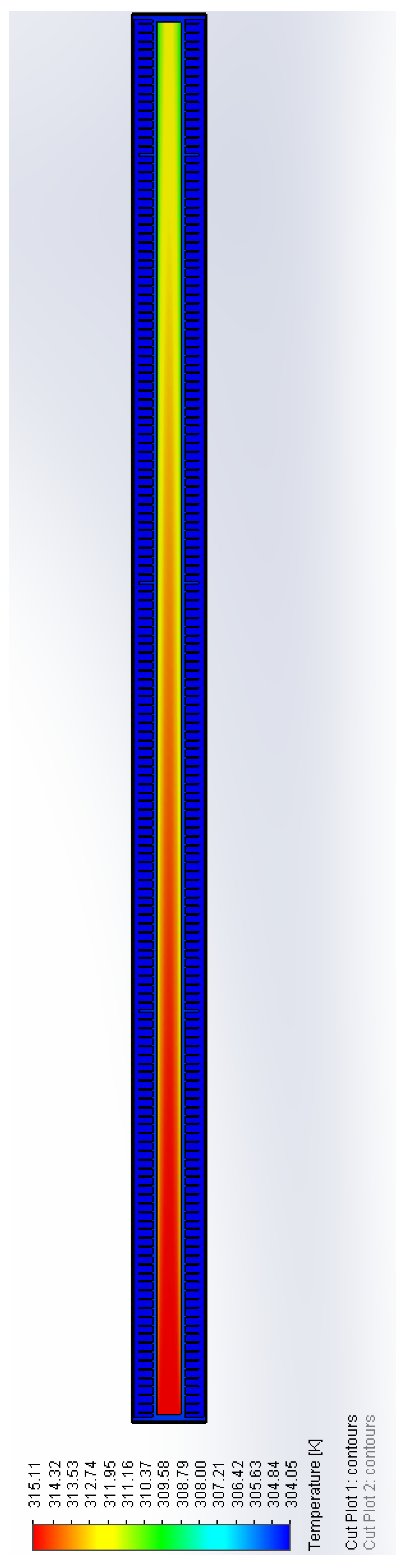
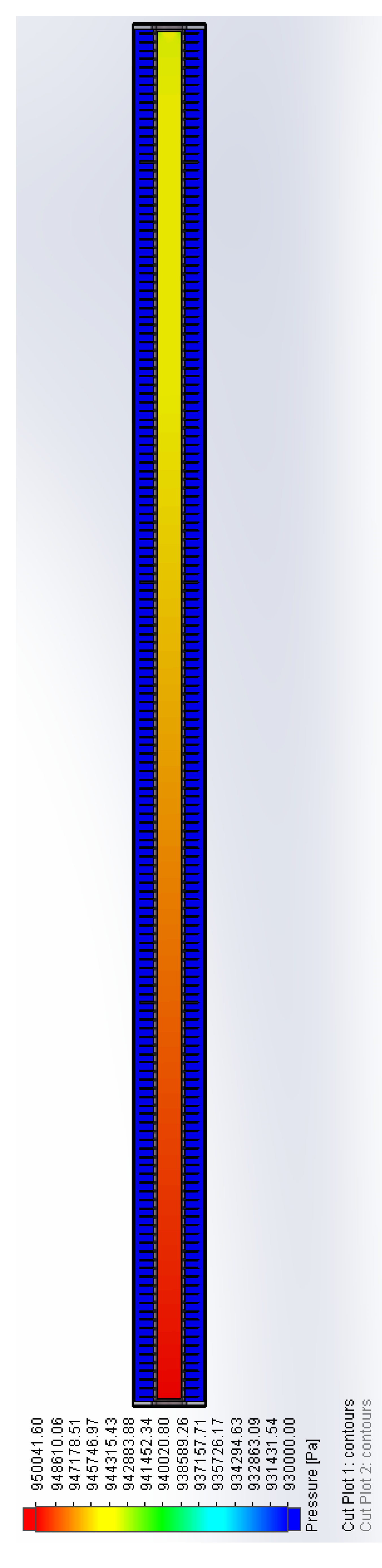
In the plot in
Figure 12, it can be seen the effective temperature drop of organic fluid R134a, obtained by simulation. As expected, the temperature drop inside the tube is higher near the walls than the central area, the average values verify the theoretical calculation. The same assessment are made for the pressure drop in the organic fluid R134a (
Figure 13).
Figure 12.
Section side view of temperature plot with the scale of measurement optimize for R134a internal trend.
Figure 12.
Section side view of temperature plot with the scale of measurement optimize for R134a internal trend.
Figure 13.
Section side view of pressure plot, with the scale of measurement optimize for R134a internal trends.
Figure 13.
Section side view of pressure plot, with the scale of measurement optimize for R134a internal trends.
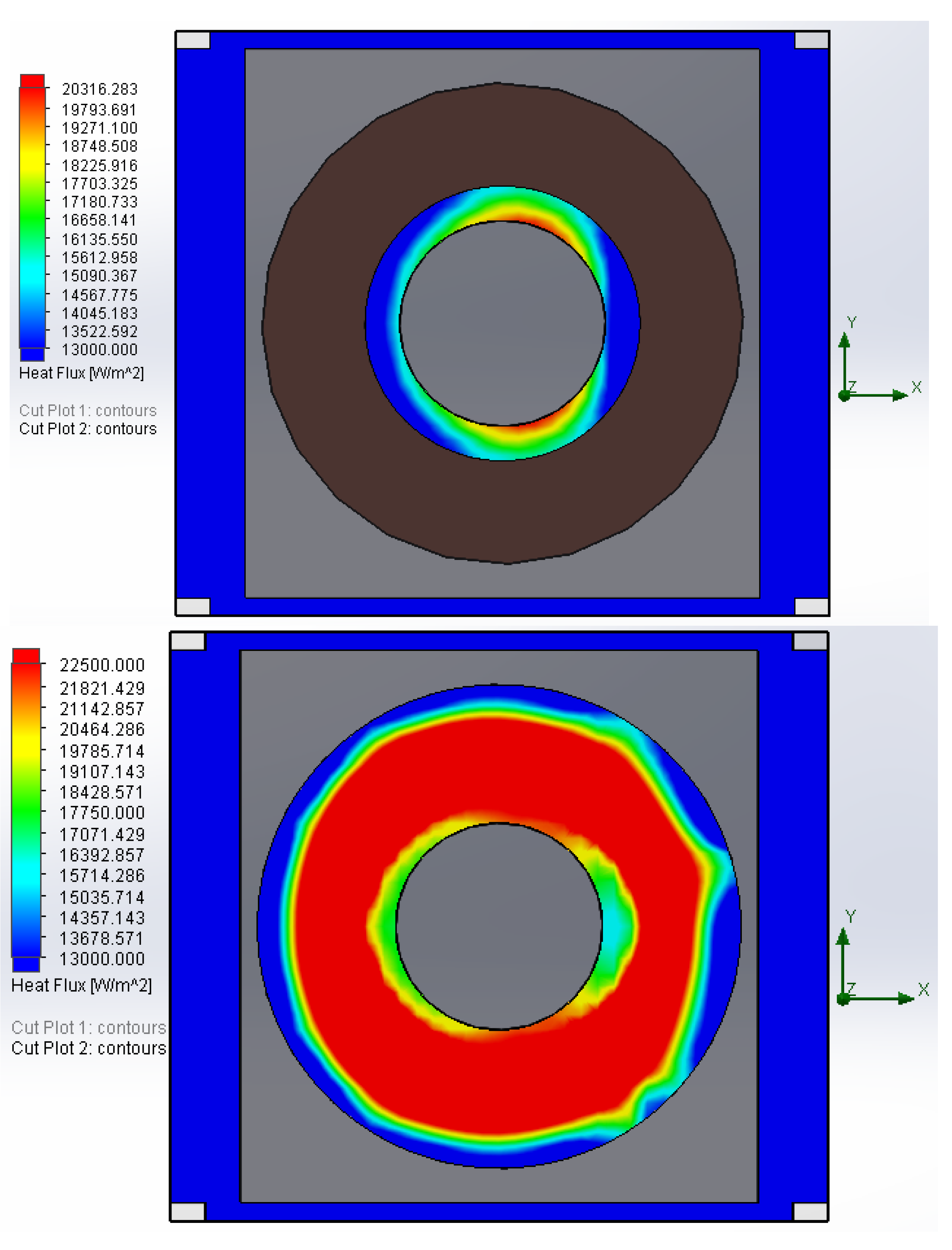
The diagrams in
Figure 14 show the heat exchange performance in the pipe, once the internal heat flux in the tube and fin sections is assessed. The heat flux reaches higher values in the fin than those detected in the pipeline, and the value around 22,500 W/m
2 remains approximately constant along almost the totality of the fin, but with a significant decrease of 50% in the outer part. The integral calculations carried out on the internal and external areas of the element, are necessary for evaluation of the heat transfer rate in Watts. Theoretical values and the simulation values are very close to each other (
Table 11), this shows a good element design, and, often, the theoretical calculations provide a safety margin in the operation.
Figure 14.
Heat flux tube plot, and heat flux fin zone plot.
Figure 14.
Heat flux tube plot, and heat flux fin zone plot.
Table 11.
Simulation results.
Table 11.
Simulation results.
| Variables | Theoretical value | Simulation value |
|---|
| Outlet R134a temperature (°K) | 310.66 | 311 |
| Pressure drop R134a (Pa) | 7215 | 6402 |
| Thermal power exchanged (W) | 109.04 | 109.42 |
Using this CFD study the pressure drop for the cooling water side is calculated (55 Pa) for the single pipe, and for the total condenser we have:
They represent about the 11.3% of the inlet pressure, but there are no additional problems because the inlet cooling water pressure is fixed to 150,000 Pa.
7.3. Simulation of Mechanical Stress
In this section the mechanical stress, deriving from contemporary internal pressure in the tube, and its thermal expansion, has been evaluated. In this case, the program used is the SolidWorks Simulation.
The calculation mesh is characterized by:
24,987 elements,
Mesh based on curvature ( the mesh tool creates more elements in higher-curvature areas automatically),
Four Jacobian points (the number of integration points to be used in checking the distortion level of tetrahedral elements).
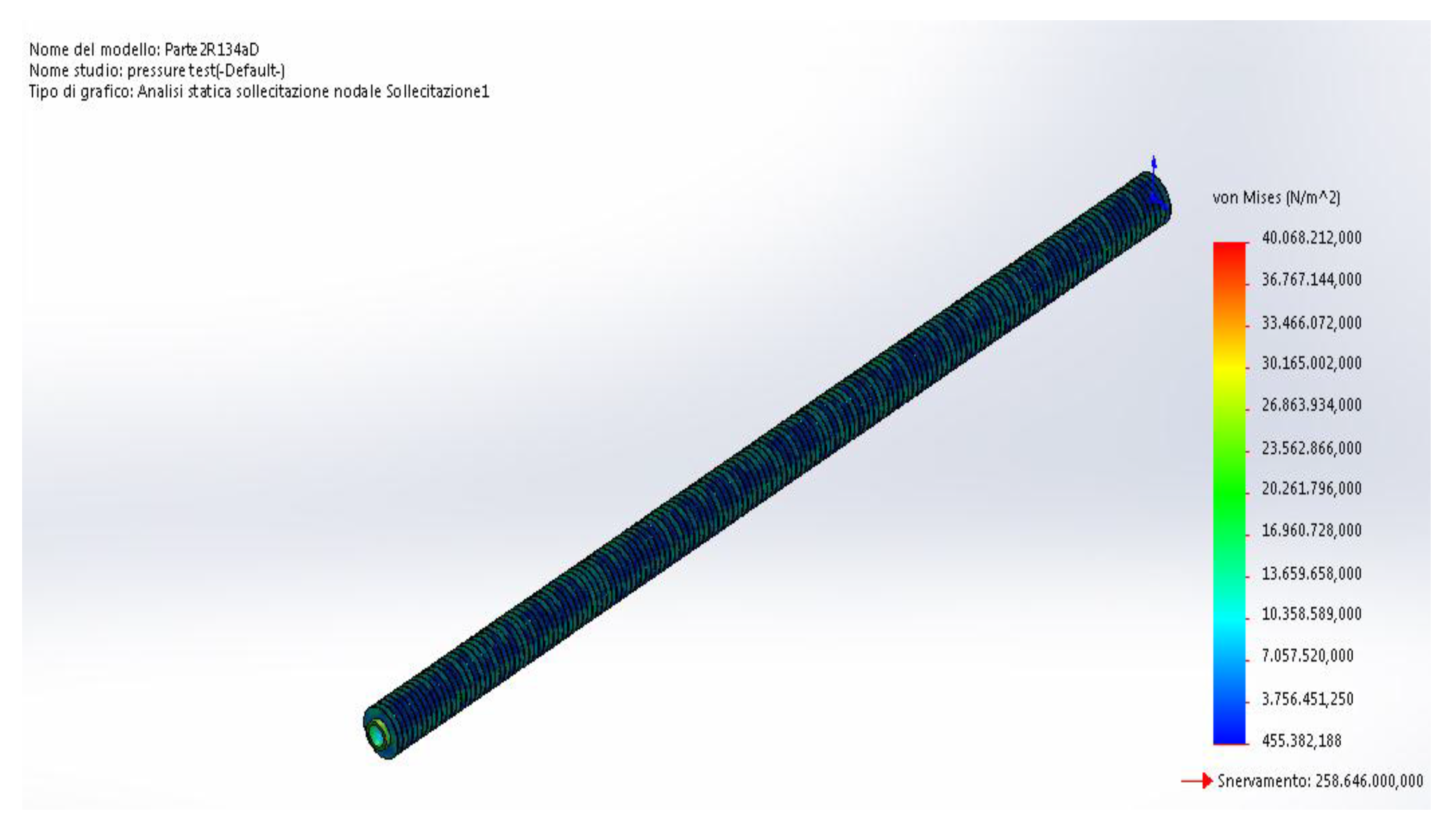
The used values in the simulation are reported as follows:
Inlet pressure = 950,000 Pa,
Maximum temperature = 305 K (for the inner tube surface),
Maximum stress = 40 × 106 N/m2,
Yield strength = 258,646,000 N/m2.
Figure 15 shows the diagram of the mechanical stress, evaluated with the Von Mises stress criterion. The principle is based on the Von Mises-Hencky theory, also known as the theory of cutting energy or maximum distortion energy theory. In terms of principal stress σ
1, σ
2 and σ
3 the Von Mises stress is expressed as [
23]:
Figure 15.
Diagram of mechanical stress with the Von Mises theory.
Figure 15.
Diagram of mechanical stress with the Von Mises theory.
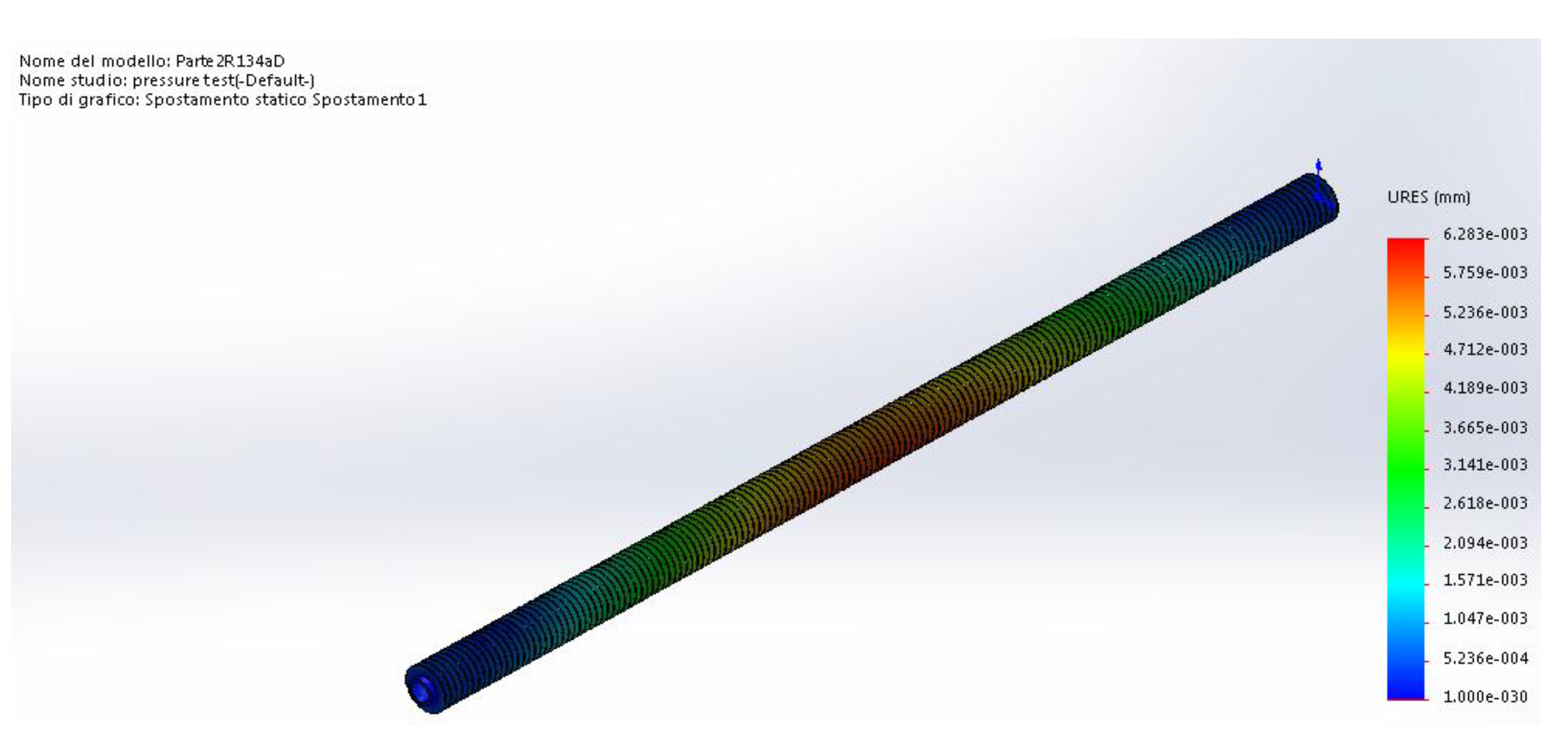
The element therefore has no point of dangerous mechanical stress. A further study was made on the thermal expansion suffered by the tube. The smaller distance is equal to 1 mm, and the maximum displacement for the thermal expansion is about 0.006 mm, so we are largely in a safe operation zone (
Figure 16).
Figure 16.
Diagram of resulting displacement.
Figure 16.
Diagram of resulting displacement.
8. Condenser Design Results for the R245fa System
The condenser for the R245fa cycle shown in
Section 4 has been designed using the same considerations employed in the previous case and presented in
Section 5 and
Section 6. Geometry values estimation has been carried out in the exact same way as the R134a case shown in
Section 7. In
Figure 17 the thermal scheme of condensation process are shown. The condenser geometric characteristics for the R245fa configuration, are given in
Table 12,
Table 13,
Table 14 and
Table 15.
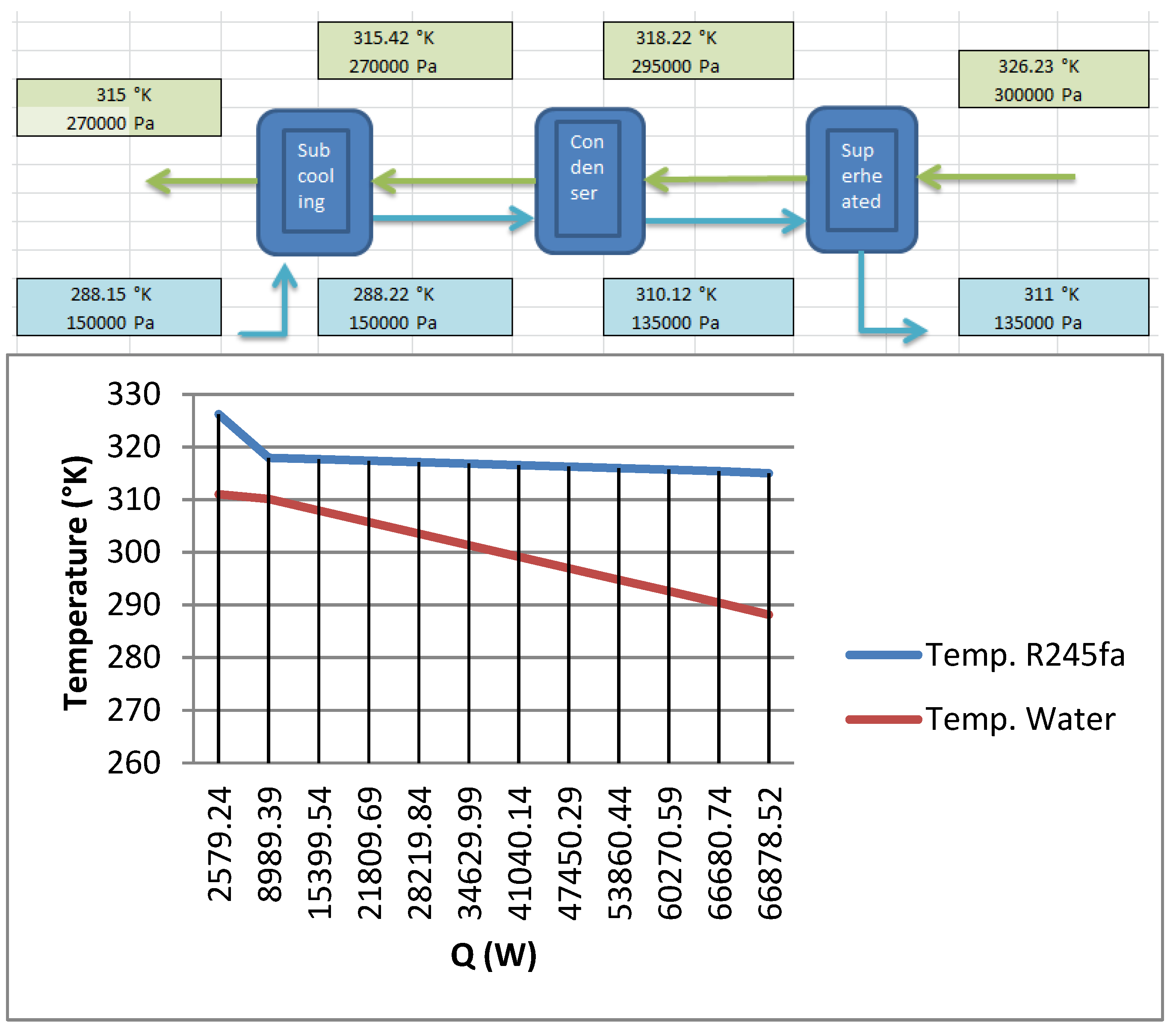
Figure 17.
R245fa thermal scheme.
Figure 17.
R245fa thermal scheme.
Table 12.
Geometric characteristics of R245fa component.
Table 12.
Geometric characteristics of R245fa component.
| Characteristics | Value | Unit |
|---|
| Inner tube diameter | 8 | mm |
| Tube thickness | 1 | mm |
| Fins distance | 2 | mm |
| Fins height | 3 | mm |
| Fins thickness | 0.3 | nm |
| Tube distance “Pt” | 19 | mm |
| Tube distance “Pl” | 19 | mm |
| Tubes number “Ns” | 17 | - |
| Tubes number “Nr” | 15 | - |
| Total tubes number | 255 | - |
Table 13.
Main dimensions of R245fa component.
Table 13.
Main dimensions of R245fa component.
| Dimensions | Value | Unit |
|---|
| Component length “L1” | 290 | mm |
| Component width “L2” | 335 | mm |
| Component height “L3” | 300 | mm |
Table 14.
Thermal power exchanged.
Table 14.
Thermal power exchanged.
| Thermal power | Value | Unit |
|---|
| Q “Sub-cooling” | 197.78738 | W |
| Q “Condensing” | 64105.018 | W |
| Q “Superheated” | 2579.2371 | W |
| Q “Total” | 66882.042 | W |
Table 15.
Area of heat exchange.
Table 15.
Area of heat exchange.
| Area | Value | Unit |
|---|
| Area “Sub-cooling” | 0.008925 | m2 |
| Area “Condensing” | 1.53173 | m2 |
| Area “Superheated” | 0.205966 | m2 |
| Area “Total” | 1.746621 | m2 |
The overall value of the heat transfer coefficient is:
The total pressure drop is the sum of the pressure drop in each phase:
It represent a loss of 9.80% respect inlet pressure. The inner area of the tubes available for the thermal exchange, in total is:
Then this area is increased by 6% compared to the area required, (derived from theoretical calculation), in this way the sizing of the component is validated. The effectiveness mean of the element is 75%. In this preliminary study, it can be noticed that the heat exchange area for the components with R245fa is greater than the component with R134a. Because the purpose of the study is to obtain the maximum compactness of the components, the solution with R245fa fluid has been considered not-so convenient in our case. For this reason, only the data for the design and the thermodynamic performance have been reported, and studies or additional CFD simulations were not presented, although they have been carried out.
9. Conclusions
A preliminary design of a compact condenser in an ORC system for small size waste heat recovery has been carried out. The performance of the ORC cycle has been simulated with the CAMEL-Pro™ software considering two different organic working fluids. The first result is that the system technical feasibility has been confirmed. Then a tube and fins type condenser has been designed, under a set of specifications, derived from the previous simulations, and always keeping in mind the requirement of the highest possible compactness. The condenser model is drawn and assembled using the commercial software to verify the correct design. Additionally, FEM and CFD studies were carried out ensure the mechanical strength of the components and confirm the heat exchange value. The designed components are quite compact and can be used in static or dynamic systems. For dynamic systems, such as common motor vehicles or naval vehicles, an additional radiator for heat dissipation can be provided. In this first phase, the same car radiator is used, while for nautical vehicles is possible to disperse the thermal power in heat exchanger placed in the water. The evaluation of these possibilities are left for further studies in the future. The next step is perform a good and complete CFD analysis for improve the heat exchange parts, the geometry of the fins and their arrangement, and to increase the heat flow. Also future studies with non-smooth piping, so the internal turbulence values are increased, the Nusselt number is increased and thus the heat exchange. Moreover in the near future an important development step will be the presentation of new more efficient ORC fluids by manufacturers [
24].


