
Research on Power Device Fault Prediction of Rod Control Power Cabinet Based on Improved Dung Beetle Optimization–Temporal Convolutional Network Transfer Learning Model
Abstract
:1. Introduction
2. Algorithm Theoretical Foundation
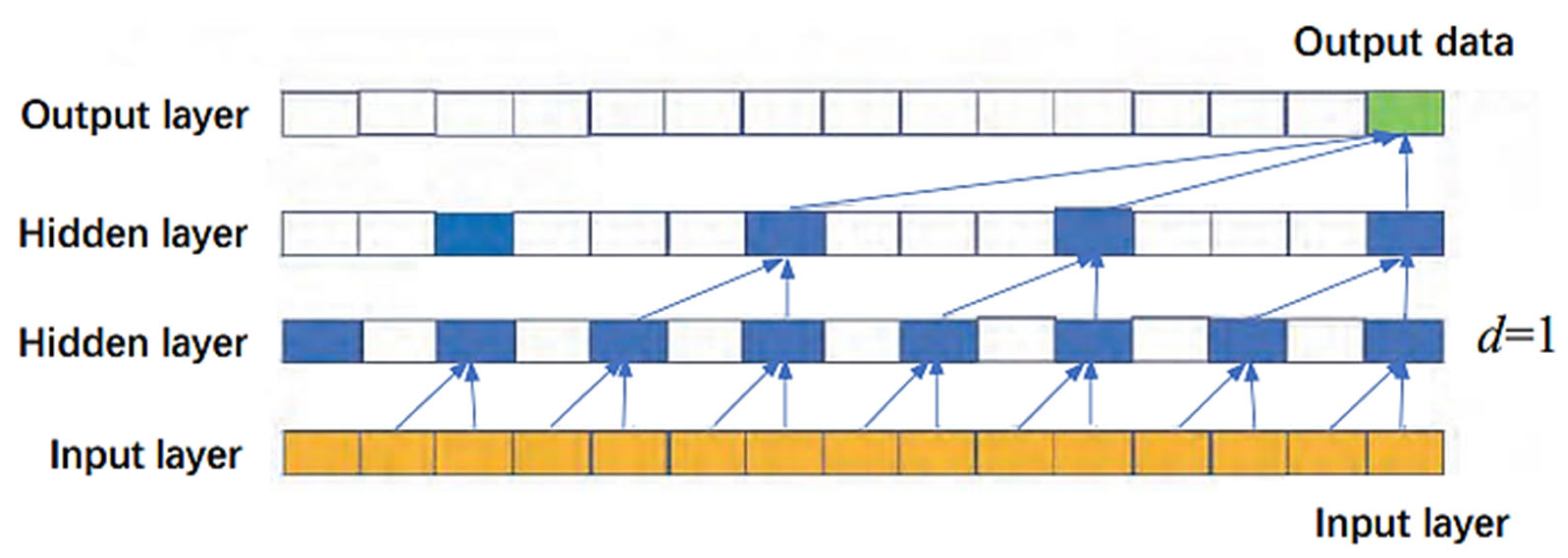
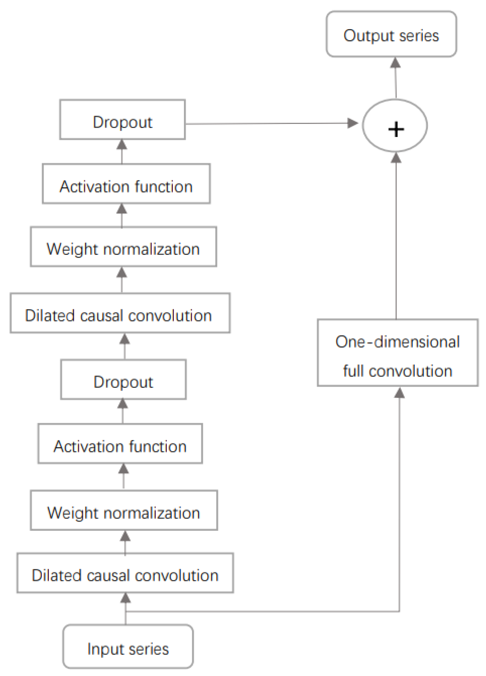
2.1. TCN Model
2.2. KPCA Principles
2.3. Transfer Learning
2.4. Dung Beetle Optimization Algorithm
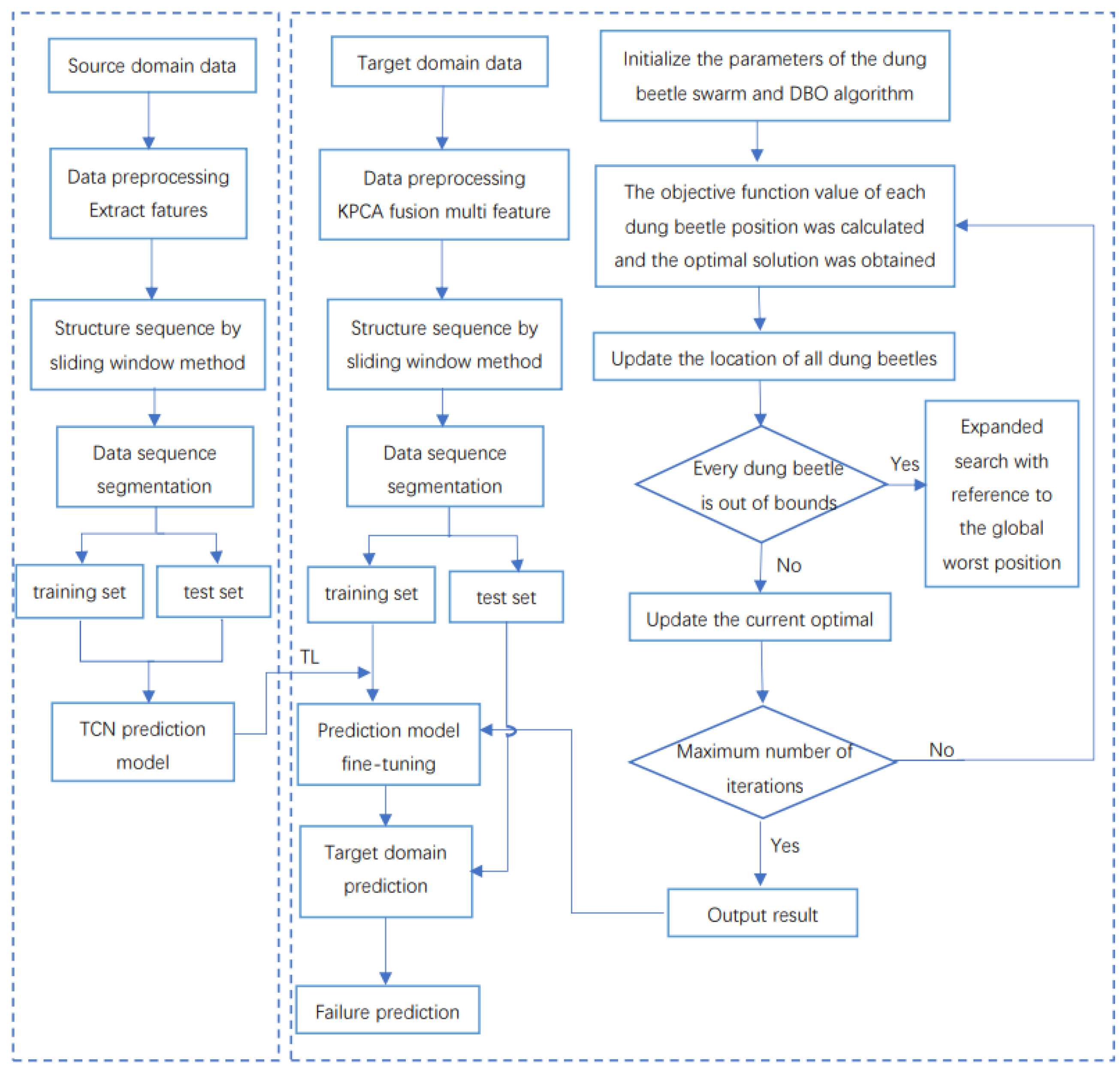
3. DBO-TCN Optimized Transfer Learning Model
3.1. TCN Modeling
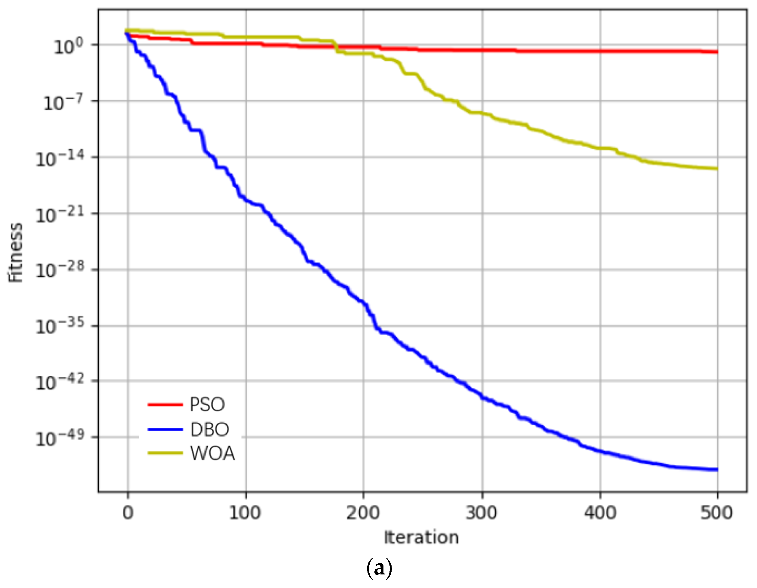
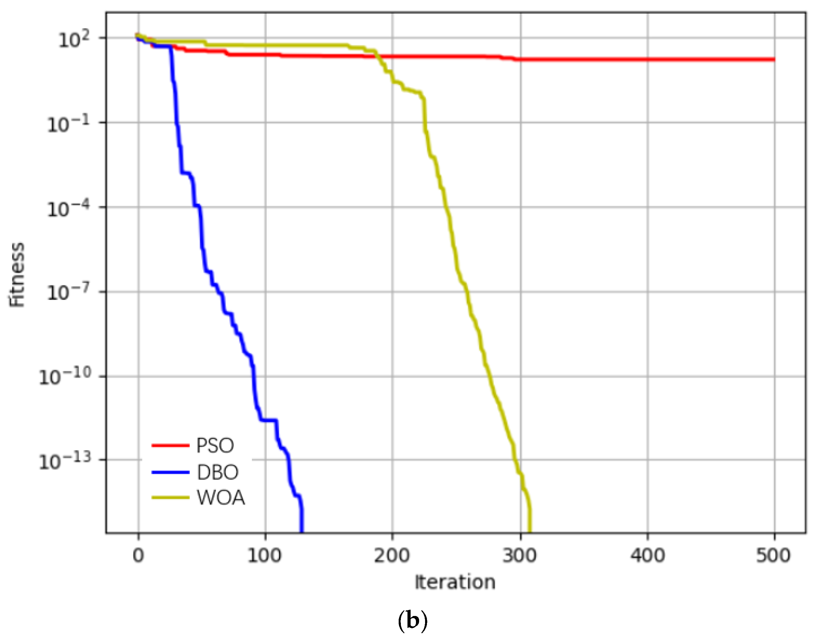
3.2. DBO Performance Testing
3.3. DBO-TCN Optimized Transfer Learning Model
4. Model Verification
4.1. Data Presentation
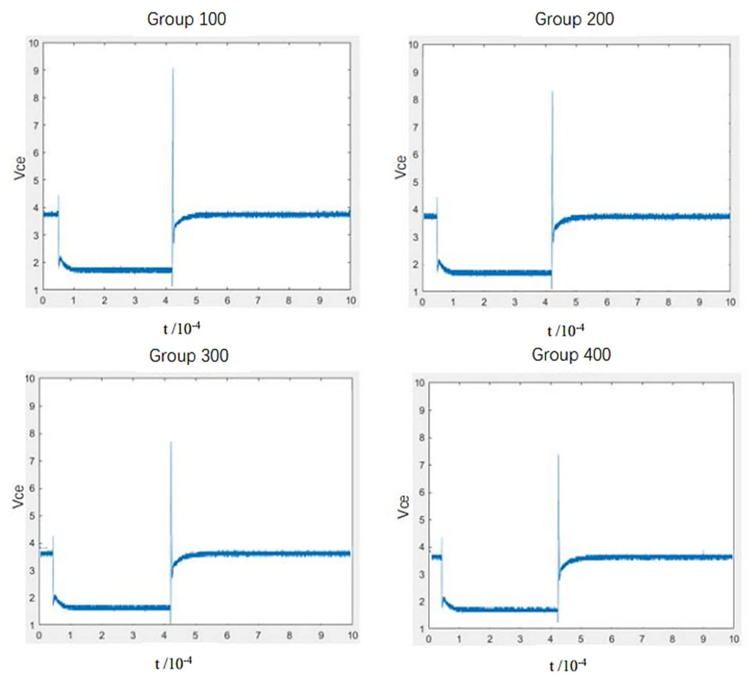
- (1)
- Accelerated thermal overstress aging with a square signal at the gate. A square signal with a frequency of 10 kHz, a duty cycle of 40%, and an amplitude of 10 V was applied to the gate of the IRG4BC30K power device, and the temperature of the package was controlled to be 268–270 °C. In this case, the device was subjected to continuous overcurrent and a high-temperature aging test. The IGBT devices were continuously turned on and off, and the temperature of the package rose under the control of a drive mode with a fixed frequency and fixed pulse width. The driving mode with a fixed-frequency- and fixed-pulse-width control signal was turned off when the maximum temperature threshold was reached and was turned on again when the temperature was lower than the minimum temperature threshold. After 418 sets of the turn-on/turn-off test, the IGBTs latched up and the device failed. Each turn-on/turn-off set contained 100,000 collector–emitter voltage data.
- (2)
- Accelerated thermal overstress aging with a square signal at the gate and SMU. During the experiment, the emitter was connected to the ground wire of the power supply, and the collector and the resistor were connected in series to the positive lead of the power supply. The gate was driven by a high-speed amplifier that amplifies the output of a function generator to realize a jump in the device supply voltage from 2.5 V to 5.5 V with an amplitude of 0.5 V. A fixed-frequency- and fixed-pulse-width signal with a duty cycle of 40%, frequency of 1 kHz, and amplitude of 8 V was applied to the gate to control the opening of the IGBT device.
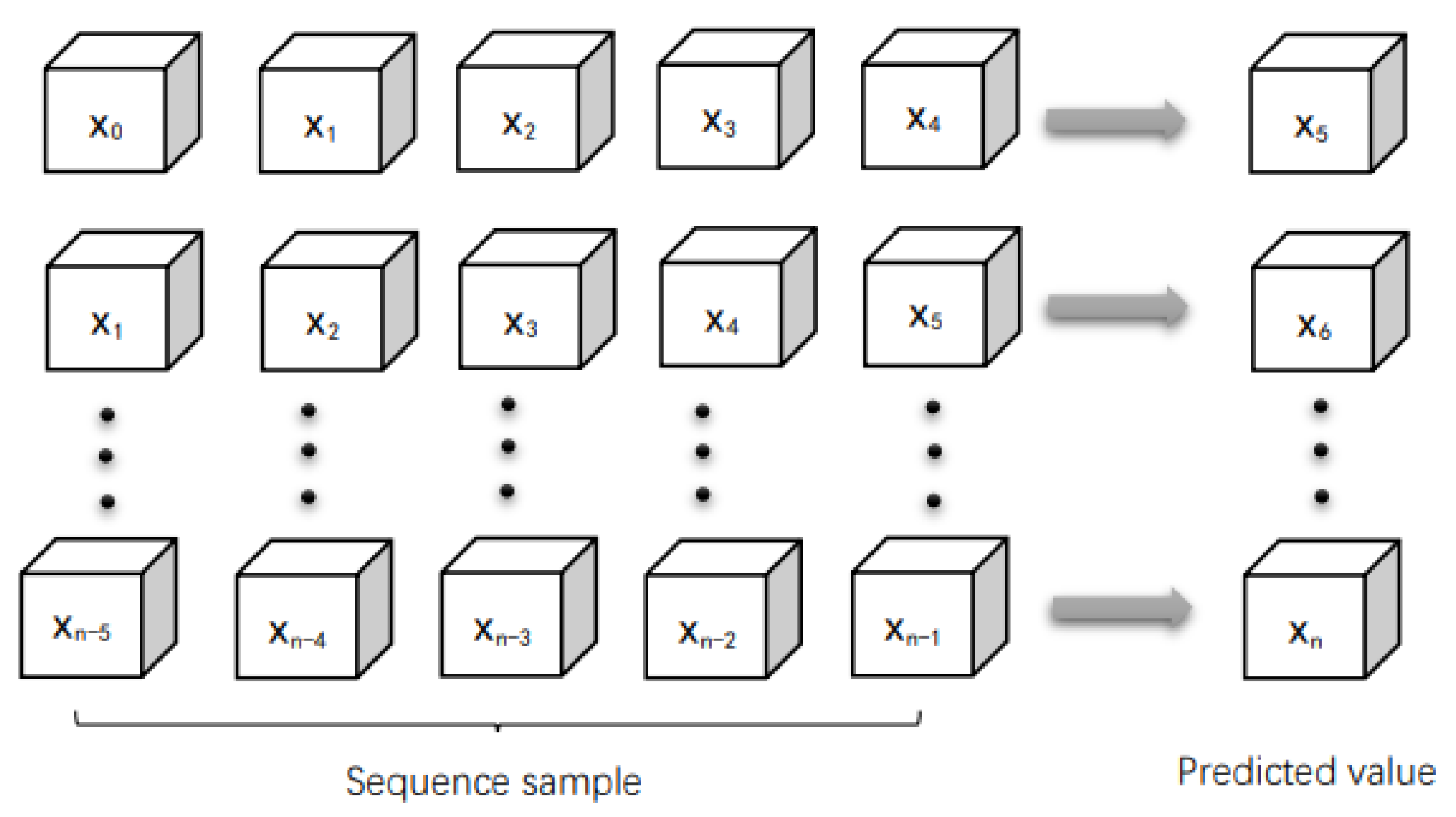
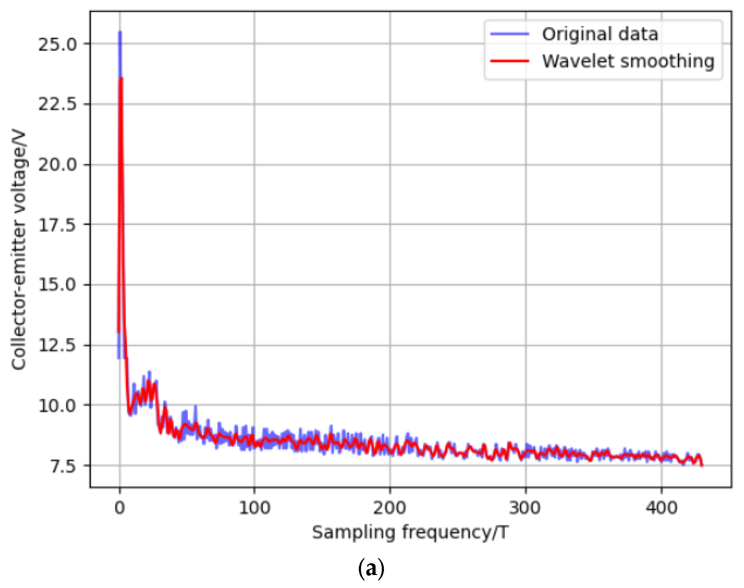
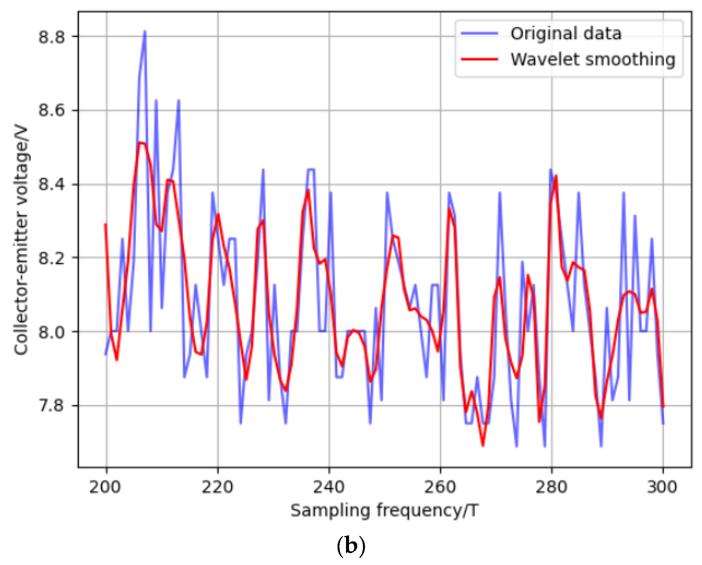
4.2. Data Pre-Processing
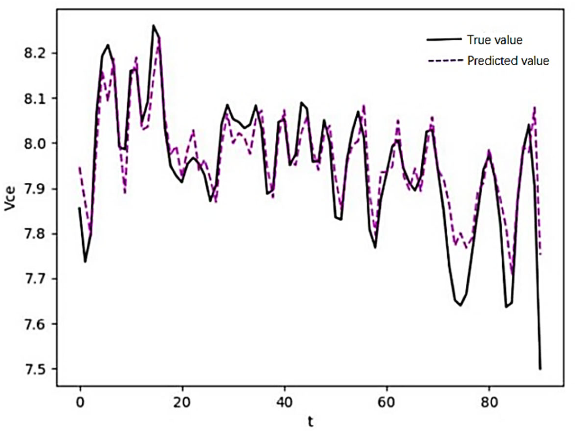
4.3. TCN-Based IGBT Fault Prediction Modeling
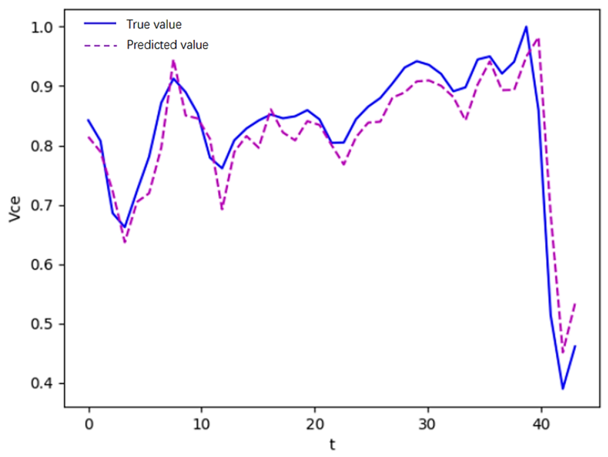
4.4. Optimal Transfer Learning Model of IGBT Based on DBO-TCN
- (1)
- The TCN prediction model was obtained using the experimental data of accelerated thermal overstress aging with a square signal at the gate as the source domain.
- (2)
- Some network structure and weight parameters of the TCN model were frozen to keep them unchanged.
- (3)
- The DBO optimization algorithm was used to optimize the learning rate of the transfer model, the number of nodes in the hidden layer, and the number of training times, so as to obtain the parameters suitable for the samples in the target domain, and then the IGBT fault prediction model of transfer learning was obtained.
5. Conclusions
Author Contributions
Funding
Data Availability Statement
Conflicts of Interest
References
- Xu, Y.; Li, T.; Wang, C. Application of IGBT in rod control system of nuclear power plant. Autom. Instrum. 2014, 35, 41–43+46. [Google Scholar]
- Zhong, Z.; Wang, Y.; Huang, Y.; Xiao, D.; Xia, P.; Liu, C. Probabilistic sparse self-attention-based prediction of IGBT module remaining life across operating conditions. J. Shanghai Jiao Tong Univ. 2023, 57, 1005–1015. [Google Scholar]
- Alghassi, A.; Perinpanayagam, S.; Samie, M. Stochastic RUL Calculation Enhanced with TDNN-Based IGBT Failure Modeling. IEEE Trans. Reliab. 2016, 65, 558–573. [Google Scholar] [CrossRef]
- Oh, H.; Han, B.; McCluskey, P.; Han, C.; Youn, B.D. Physics of Failure, Condition Monitoring, and Prognostics of Insulated Gate Bipolar Transistor Modules: A Review. IEEE Trans. Power Electron. 2015, 30, 2413–2426. [Google Scholar] [CrossRef]
- Wu, Z.; Bai, H.; Yan, H.; Zhan, X.; Guo, C.; Jia, X. Intelligent Fault Diagnosis Method for Gearboxes Based on Deep Transfer Learning. Processes 2023, 11, 68. [Google Scholar] [CrossRef]
- He, B. Failure Mechanism Analysis of IGBT Based on Comsol Multiphysics Field Coupling Simulation; Harbin Institute of Technology: Harbin, China, 2021. [Google Scholar]
- Huang, K. Research on IGBT Module Performance Degradation and Fault Prediction Technology; Southwest Jiaotong University: Chengdu, China, 2022. [Google Scholar]
- Yuan, M.; Yin, Z.; Luo, P.; Zhang, Y. MPCC-based open-circuit fault diagnosis method for inverter IGBTs in permanent magnet synchronous motor drive systems. Electr. Drives 2023, 53, 25–31+54. [Google Scholar]
- Górecki, P.; Górecki, K.; Zarębski, J. Accurate Circuit-Level Modelling of IGBTs with Thermal Phenomena Taken into Account. Energies 2021, 14, 2372. [Google Scholar] [CrossRef]
- Held, M.; Jacob, P.; Nicoletti, G.; Scacco, P.; Poech, M.H. Fast Power Cycling Test for Insulated Gate Bipolar Transistor Modules in Traction Application. Int. J. Electron. 1999, 86, 1193–1204. [Google Scholar] [CrossRef]
- Bayerer, R.; Hermann, T.; Licht, T.; Lutz, J.; Feller, M. Model for Power Cycling Lifetime of IGBT Modules-Various Factors Influencing Lifetime. In Proceedings of the 5th International Conference on Integrated Power Electronics Systems, Nuremberg, Germany, 11–13 March 2008; pp. 1–6. [Google Scholar]
- Zhou, C.; Gao, B.; Yang, H.; Zhang, X.; Liu, J.; Li, L. Junction Temperature Prediction of Insulated Gate Bipolar Transistors in Wind Power Systems Based on an Improved Honey Badger Algorithm. Energies 2022, 15, 7366. [Google Scholar] [CrossRef]
- Zhou, A.; Mahemuti, P.; Li, G.; Zhao, Z.; Liu, H. Study on IGBT life prediction based on SMA-Elman. Microelectron. Comput. 2023, 40, 117–124. [Google Scholar]
- Ismail, A.; Saidi, L.; Sayadi, M.; Benbouzid, M. A New Data-Driven Approach for Power IGBTs Remaining Useful Life Estimation Based On Feature Reduction Technique and Neural Network. Electronics 2020, 9, 1571. [Google Scholar] [CrossRef]
- Bai, S.; Kolter, J.Z.; Koltun, V. An empirical evaluation of generic convolutional and recurrent networks for sequence modeling. arXiv 2018, arXiv:1803.01271. [Google Scholar]
- Gao, X.; Ma, D.; Han, H.; Gao, H. Fault prediction of complex industrial processes based on DAE and TCN. J. Instrum. 2021, 42, 140–151. [Google Scholar]
- Jin, S.; Si, F.; Dong, Y.; Ren, S. A Data-Driven Kernel Principal Component Analysis–Bagging–Gaussian Mixture Regression Framework for Pulverizer Soft Sensors Using Reduced Dimensions and Ensemble Learning. Energies 2023, 16, 6671. [Google Scholar] [CrossRef]
- Wang, J.; Chen, Y. Introduction to Transfer Learning, 2nd ed.; Electronic Industry Press: Beijing, China, 2022. [Google Scholar]
- Xue, J.; Bo, S. Dung beetle optimizer: A new meta-heuristic algorithm for global optimization. J. Supercomput. 2023, 79, 7305–7336. [Google Scholar] [CrossRef]
- Han, H. Research on IGBT Fault Prediction Based on Deep Learning; Beijing Jiaotong University: Beijing, China, 2019. [Google Scholar]
- Leng, L.; Fu, J.; Ning, B. Study on IGBT time series prediction based on SSA-LSTM model. Semicond. Technol. 2023, 48, 66–72. [Google Scholar]
- Deepak, M.; Rustum, R. Review of Latest Advances in Nature-Inspired Algorithms for Optimization of Activated Sludge Processes. Processes 2023, 11, 77. [Google Scholar] [CrossRef]
- Li, W.; Zhang, W.; Liu, B.; Guo, Y. The Situation Assessment of UAVs Based on an Improved Whale Optimization Bayesian Network Parameter-Learning Algorithm. Drones 2023, 7, 655. [Google Scholar] [CrossRef]
- Yang, P.; Zhang, J.; Wang, X.; He, Z.; Zheng, G. Simulation and optimization of nuclear reactor rod-controlled power supply circuit. Nucl. Technol. 2020, 43, 39–45. [Google Scholar]
- Zhang, M.; Wang, Q.; Yu, Y. IGBT fault prediction under thermal stress based on GRU and PCA-TL. Sci. Technol. Eng. 2023, 23, 4654–4659. [Google Scholar]
- Sonnenfeld, G.; Goebel, K.; Celaya, J.R. An agile accelerated aging, characterization and scenario simulation system for gate controlled power transistors. In Proceedings of the 2008 IEEE International Automatic Testing Conference, AUTOTESTCON, Salt Lake City, UT, USA, 8–11 September 2008; pp. 208–215. [Google Scholar]


| Function | Search Area | Optimal Value |
|---|---|---|
| [−100, 100] | 0 | |
| [−5.12, 5.12] | 0 |
| Function | DBO | PSO | WOA | ||||||
|---|---|---|---|---|---|---|---|---|---|
| Optimal Value | Standard Deviation | Average Value | Optimal Value | Standard Deviation | Average Value | Optimal Value | Standard Deviation | Average Value | |
| 7.81 × 10−54 | 8.50 × 10⁻²⁸ | 3.19 × 10⁻²⁹ | 1.28 × 10⁻¹ | 2.07 × 10⁻¹ | −9 × 10⁻³ | 3.29 × 10⁻¹⁶ | 1.05 × 10⁻⁸ | 4.77 × 10⁻¹⁰ | |
| 0 | 5.56 × 10⁻¹⁰ | −5.90 × 10⁻¹¹ | 1.61 × 101 | 1.035 | −1.2 × 10⁻² | 0 | 5.66 × 10⁻¹⁰ | 2.93 × 10⁻¹⁰ | |
| Model | MSE/% | RMSE/% | MAE/% |
|---|---|---|---|
| TCN | 0.36 | 6.05 | 4.7 |
| LSTM | 2.13 | 14.62 | 11.16 |
| GRU | 1.94 | 13.93 | 11.20 |
| RNN | 2.56 | 16.02 | 12.01 |
| Model | MSE/% | RMSE/% | MAE/% |
|---|---|---|---|
| DBO-TCN transfer learning model | 0.24 | 4.93 | 3.84 |
| Target-domain-retraining TCN model | 0.95 | 9.79 | 8.29 |
| LSTM transfer learning model | 2.21 | 14.88 | 11.15 |
| GRU transfer learning model | 2.25 | 15.02 | 11.29 |
| RNN transfer learning model | 3.02 | 17.39 | 12.97 |
Disclaimer/Publisher’s Note: The statements, opinions and data contained in all publications are solely those of the individual author(s) and contributor(s) and not of MDPI and/or the editor(s). MDPI and/or the editor(s) disclaim responsibility for any injury to people or property resulting from any ideas, methods, instructions or products referred to in the content. |
© 2024 by the authors. Licensee MDPI, Basel, Switzerland. This article is an open access article distributed under the terms and conditions of the Creative Commons Attribution (CC BY) license (https://creativecommons.org/licenses/by/4.0/).
Share and Cite
Ye, L.; Chen, Z.; Liu, J.; Lin, C.; Jian, Y. Research on Power Device Fault Prediction of Rod Control Power Cabinet Based on Improved Dung Beetle Optimization–Temporal Convolutional Network Transfer Learning Model. Energies 2024, 17, 447. https://doi.org/10.3390/en17020447
Ye L, Chen Z, Liu J, Lin C, Jian Y. Research on Power Device Fault Prediction of Rod Control Power Cabinet Based on Improved Dung Beetle Optimization–Temporal Convolutional Network Transfer Learning Model. Energies. 2024; 17(2):447. https://doi.org/10.3390/en17020447
Chicago/Turabian StyleYe, Liqi, Zhi Chen, Jie Liu, Chao Lin, and Yifan Jian. 2024. "Research on Power Device Fault Prediction of Rod Control Power Cabinet Based on Improved Dung Beetle Optimization–Temporal Convolutional Network Transfer Learning Model" Energies 17, no. 2: 447. https://doi.org/10.3390/en17020447