
Computational Study of Deflagration-to-Detonation Transition in a Semi-Confined Slit Combustor

1
Department of Combustion and Explosion, Semenov Federal Research Center for Chemical Physics (FRC), Moscow 119991, Russia
2
Institute of Laser and Plasma Technologies, National Research Nuclear University MEPhI, Moscow 115409, Russia
*
Author to whom correspondence should be addressed.
Energies 2023, 16(20), 7028; https://doi.org/10.3390/en16207028
Submission received: 3 August 2023
/
Revised: 11 September 2023
/
Accepted: 28 September 2023
/
Published: 10 October 2023
(This article belongs to the Section B: Energy and Environment)
Abstract
:Systematic three-dimensional numerical simulations of flame acceleration and deflagration-to-detonation transition (DDT) in a semi-confined flat slit combustor are performed. The combustor is assumed to be partly filled with the stoichiometric ethylene–oxygen mixture at normal pressure and temperature conditions. The objective of the study is to reveal the conditions for DDT in terms of the minimum height of the combustible mixture layer in the slit, the maximum dilution of the mixture with nitrogen and the maximum slit width. The results of the calculations are compared with the available experimental data. The calculation results are shown to agree satisfactorily with the experimental data on the slit-filling dynamics, flame structure, the occurrence of the preflame self-ignition center, DDT, and detonation propagation. DDT occurs in the layer at a time instant when the flame accelerates to a velocity close to 750 m/s. DDT occurs near the slit bottom due to the formation of the self-ignition center ahead of the leading edge of the flame as a result of shock wave reflections from the walls of injector holes at the slit bottom and from the corners of the conjugation of the slit bottom and side walls. The decrease in the height of the mixture layer, the dilution of the mixture with nitrogen, and the increase in the slit width are shown to slow down flame acceleration in the slit and increase the DDT run-up distance and time until DDT failure. The obtained results are important for determining the conditions for mild initiation of detonation via DDT in semi-confined annular RDE combustors.
1. Introduction
The combustion chamber (combustor) of a Rotating Detonation Engine (RDE) is usually an annular slit between the central body and the outer wall [1]. When the RDE is started, the slit is first filled with the fuel and oxidizer followed by detonation initiation leading to the formation of a single detonation wave or multiple detonation waves continuously circulating in the combustor, while the detonation products continuously outflow through the RDE nozzle into the ambience. As a means of detonation initiation, either strong or weak energy sources can be used. The strong sources are electrical arc discharges, explosive charges, predetonators, etc., creating a strong shock wave in the fuel mixture. Such energy sources can lead to the direct (“strong”) initiation of detonation. The weak energy sources are spark plugs, hot wires, prechambers, pyro charges, etc. igniting the fuel mixture with the formation of a propagating flame. Under certain conditions, the arising flame can accelerate and lead to a “mild” detonation initiation via a deflagration-to-detonation transition (DDT). Several important circumstances should be taken into account when applying either of these approaches to detonation initiation. First, for the guaranteed detonation initiation, it is necessary to have a sufficient volume of the fuel mixture in the RDE combustor. Second, the process of detonation initiation can be accompanied by the displacement of the fuel mixture to the ambience through the RDE nozzle, creating a risk of a devastating external explosion.
Since detonation initiation in the RDE combustor leads to a significant pressure rise for a very short time [2,3], a large margin of safety is usually envisaged in the design of experimental RDEs. When transitioning to RDE prototypes, the straightforward solution for increasing the thrust-to-weight ratio is to reduce the engine mass by reducing the margin of safety. The minimal margin of safety can be ensured by the use of the “mild” initiation of detonation. As for the “strong” initiation, it must be excluded, as it is accompanied by a destructive explosion of the excess volume of the fuel mixture inside and outside the RDE.
Voitsekhovsky [4] was apparently the first who studied the propagation of a stationary detonation wave in an annular slit with the lateral expansion of detonation products. Detonation propagation in the flat semi-confined layer of explosive gas (mixtures of H2, CH4, C2H6, or C3H8 with oxygen) surrounded by inert gas (air or helium) was studied both theoretically and experimentally in [5]. It was shown that (i) the detonation wave propagating through the layer was affected by the type of inert gas, (ii) the detonation velocity decreased with a decrease in the layer height and (iii) the detonation failed to propagate through the layer if its height was less than a certain critical (minimal) value. Experiments with flat layers of H2–O2 mixtures of various compositions were reported in [6]. In addition, a theory of layered detonation with a finite reaction rate was proposed. The detonation velocity deficit in a layer of near-critical height was shown to reach 8–10%. Similar studies with longer layers were reported in [7]. The maximum deficit of the detonation velocity in a layer of near-critical height reached 17%, i.e., approximately twice higher than found in [6]. The latter meant that the rate of detonation decay in long layers of a near-critical height was rather low. Detonation propagation in layers of the stoichiometric H2–O2 mixture was simulated numerically in a two-dimensional approximation [8]. The propagation of a detonation wave was shown to become unsteady (pulsating or damping) with a decrease in the layer height.
There are a large number of research works on detonation propagation in combustible mixtures of nonuniform composition. Thus, the authors of [9,10,11,12,13,14,15,16] reported the results of systematic computational and experimental studies on the propagation of detonation in mixtures with the concentration gradient parallel to the propagation direction, whereas the authors of [17,18,19,20,21,22,23,24] reported the results of systematic computational and experimental studies on the propagation of detonation in mixtures with the concentration gradient normal to the propagation direction. The latter studies look relevant to the present research, in particular those dealing with detonation propagation in a two-layered medium with different fuel concentrations. The reflection of the induced oblique shock wave from the bounding mixture confinement was shown to change from a regular to Mach reflection with the decrease in the reactivity of the bounding mixture. When the bounding mixture was weakly detonable, the detonation initiation occurred behind the reflected shock wave.
The results of large-scale experiments with flat layers of H2–O2 mixture were reported in [25,26]. The critical height of the layer for the detonation to propagate in the self-sustaining mode under normal pressure and temperature (NPT) conditions was shown to be about 30 mm or 3 λ, where λ is the detonation cell size. The nonuniformity of the hydrogen concentration in the layer was shown to exert a significant effect on the critical height of the layer. A set of theoretical models of detonation propagation in flat and cylindrical layers bounded by inert gas was also considered [27]. The adequate description of the dynamics of self-sustaining detonation waves was shown to be attained only at a certain minimum level of model complexity. The results of numerical simulations of 2D cellular detonations in layers of H2–air mixture bounded by inert gas were reported in [28]. The critical height of the layer met the empirical criterion [1]: .
It must be noted that all mentioned studies dealt with the propagation of detonation in layers of reactive mixture. As for DDT in a layer, it was studied experimentally only in a few works [26,29,30,31]. Contrary to [26,29], where DDT was provided by installing turbulizing obstacles, DDT in [30,31] occurred in a flat-slit combustor without obstacles using nonpremixed [30] and premixed [31] ethylene–oxygen compositions diluted with nitrogen. The conditions for DDT in the stoichiometric C2H4–O2 mixtures diluted with N2 up to ~40% vol. in the semi-confined large-scale flat-slit combustor with a slit width of 5 mm were reported in [31]. The mild initiation of detonation via DDT was possible when the mixture was ignited upon reaching the critical (minimal) height of the layer.
This work is considered as the continuation of [31]. Its objective is to apply 3D numerical simulations to reveal the conditions for DDT in terms of the minimum height of the combustible mixture layer in the slit, the maximum dilution of the mixture with nitrogen, and the maximum width of the slit. The objective, the applied approach, and the obtained results are the novel and distinctive features of this work.
2. Materials and Methods
2.1. Slit Combustor
Before describing the mathematical statement of the problem and the numerical approach, it is worth briefly describing the experimental setup and procedure [31]. The slit combustor [31] was the space between two parallel plates 400 mm high and 800 mm long made of organic glass and fixed in a steel frame possessing two horizontal rows of three windows. Despite the combustor design providing the possibility of adjusting the slit width, the experiments reported in [31] were implemented with the constant slit width equal to 5 mm. The combustible mixture (ethylene–oxygen mixture diluted with nitrogen, C2H4 + 3(O2 + βN2), ) was fed into the slit combustor from a plenum 60 800 mm in size through a series of 160 injector holes (diameter 1 mm, longitudinal pitch 5 mm) uniformly distributed in the bottom plate along its centerline. The plenum was filled with a loose flame-quenching material. The left end of the combustor was a closed insulating wall with a row of 38 spark gaps mounted along the centerline of the whole slit height. The total rated energy, ( μF is the capacitance and V is the voltage), deposited by the spark discharges was approximately 10 J. Taking into account that the actual energy transferred to the combustible mixture can account for only 10% of the rated energy [32], the actual energy deposited by each spark discharge to the combustible mixture was on the level of 30 mJ, i.e., very little. The right end of the combustor was sealed with thin parchment paper before each experiment. The upper end of the combustor was open. In experiments, the slit was first blown with air and then filled with a combustible mixture from a mixer through a flow controller during the fill time providing the preset estimated height of the mixture layer, . Thereafter, upon a pause of 10 s, a voltage was applied to all spark gaps simultaneously to trigger mixture ignition. The flame/detonation propagation process was recorded by a high-speed video camera. From the video records, the place and time of detonation onset as well as the propagation velocity of the luminous front were determined.
2.2. Mathematical Statement of the Problem
The mathematical statement of the problem is based on the three-dimensional unsteady Reynolds-averaged Navier–Stokes (URANS) equations for the compressible turbulent reacting flow supplemented by the thermal and caloric equations of state of a mixture of ideal gases with variable specific heat capacities, the k-ε turbulence model and the combustion model based on the coupled Flame Tracking (FT)—Particle method (PM), as well as by the initial and boundary conditions [33]. Gas thermophysical parameters are considered variable.
2.2.1. Mean Flow Equations
The URANS equations with the turbulence model and the thermal and caloric equations of state read:
where is time; is the material derivative; ( = 1, 2, 3) is the coordinate; is the mean density; is the dynamic molecular viscosity; is the mean pressure; is the tensor of viscous stresses; is the th component of the mean velocity vector; is the th component of the pulsating velocity vector; is the thermal conductivity; is the mean total enthalpy ( is the mean static enthalpy); is the mean static temperature; is the mean mass fraction of fuel; is the molecular diffusion coefficient of fuel in the mixture; is the pulsation of the fuel mass fraction; and are the mean sources of fuel mass and energy due to chemical reactions; is the kinetic energy of turbulence; is the dissipation rate of ; is the mean-strain production term; is the dynamic turbulent viscosity; , , , , , and are the coefficients in the standard k- model; and are the mean static enthalpy and standard enthalpy of formation of the th species in the mixture ( = 1, …, , is the total number of species), respectively; is the standard temperature (298 K); is the mean mass fraction of the th species in the mixture; is the molecular mass of the th species in the mixture; and is the universal gas constant. Equation (3) implies that the mass fractions of species other than fuel are calculated based on the balances of C, H, and O elements.
The chemical sources and represent the contributions of both frontal combustion (index ), and volumetric reactions (index ):
The FT method is used for simulating the frontal combustion, i.e., the stages of flame ignition, propagation and acceleration, whereas the PM is used for simulating preflame chemical transformations with the formation of exothermic self-ignition centers (“hot spots”), DDT, and detonation.
2.2.2. Combustion Model
Flame Tracking Method
The basis of the FT method is the Huygens principle. The surface separating the fresh combustible mixture from the combustion products is represented by a set of infinitely thin flame elements. In the flow, each element moves at a velocity equal to the sum of the local flow velocity and the local flame velocity. The local flow velocity and turbulence parameters are determined by solving Equations (1)–(7). The local turbulent flame velocity, , is related to the local laminar flame velocity, , through the mass balance equation , where and are the local instantaneous specific (per unit volume) surface areas of a true wrinkled and averaged planar flame, respectively. The turbulent flame velocity, , is determined by one of the known models of turbulent combustion; it depends on the local laminar flame velocity, , and local turbulence parameters. In this work, the Shchelkin model of turbulent combustion [34] is used, which has proven itself well in solving problems of flame acceleration and DDT [35]:
where 1 is the model parameter and is the pulsating flow velocity. For , it is convenient to use precalculated look-up tables that include the dependence of on temperature, pressure, and mixture composition. Such look-up tables were developed in the FRC for mixtures of different alkane, alkene, and alkyne hydrocarbons with air and oxygen based on either detailed or overall reaction mechanisms [36]. As an example, Figure 1 demonstrates the accuracy of the look-up tables in predicting the laminar flame velocity in an ethylene–air mixture at NPT conditions.
In the FT method, the average planar flame surface is explicitly traced and the specific surface area is determined in the course of solution. Therefore, the first terms in Equations (8) and (9) are calculated straightforward as
where and are the local instantaneous density of the fresh mixture and fuel mass fraction immediately ahead of the flame surface, respectively, and is the heat effect of combustion.
Particle Method
The PM is based on the Lagrangian approach to describe the turbulent and molecular transport of momentum and scalar flow parameters: enthalpy and mass fractions of the chemical species of the mixture [40,41]. The local instantaneous state of the flow is described by a large set of notional particles. The initial position of particles is selected using a random number generator with a uniform average distribution over the interval [0, 1]. In addition to the position in space , each th notional particle possesses three components of the velocity vector , density , volume , mass fractions of chemical species , static enthalpy , and statistical weight :
Initially, certain values of all the variables consistent with the initial distributions of the corresponding mean values are set to each particle. The following set of differential equations is solved for each th particle:
where is the partial density of the th species in the th particle; is the mean pressure in the point where the th particle is currently located; is the heat flux to the th particle due to molecular thermal conductivity; is the molecular diffusion flux of the th species to the th particle; is the th component of the momentum flux vector to the th particle due to molecular viscosity; is the rate of change of the mass fraction of the th species due to chemical reactions; and is the volumetric rate of energy release in the th particle due to chemical reactions. The terms , and are determined using the standard models [40]:
where , and are the th component of the mean flow velocity vector, the mean mass fraction of the th species, and the mean static enthalpy in the point where the th particle is currently located; and 2.0 are the coefficients; is the turbulence frequency; is the stochastic function describing the effect of pressure and velocity pulsations on particle motion (here, and is the continuous stochastic variable with normal distribution satisfying the conditions and , is the Kronecker delta); and , and are the ensemble mean values:
The local instantaneous turbulence frequency and the mean pressure , required for closing Equations (14)–(17) and relationships (18)–(20), are obtained from Equations (1)–(7).
The ability to accurately determine the rates of chemical reactions in a turbulent reactive flow is the most important advantage of the PM. As a matter of fact, terms and in Equations (15) and (17) are directly determined from the known reaction mechanism using the species mass fractions and temperature in the th particle:
where is the molecular mass of the th species; , , and are the preexponential factor, temperature exponent and activation energy of the th reaction; , are the stoichiometric coefficients for the th species in the cases when it serves as a reactant and product of the th reaction, respectively; and is the total number of reactions in the reaction mechanism.
The term is calculated as:
where is the heat effect of the th chemical reaction. Using Equations (22) and (23), the contribution of volumetric reactions and in Equations (8) and (9) can be determined from:
Thus, no hypotheses on the influence of turbulent fluctuations of temperature and species concentrations on the mean reaction rate is invoked. Note that the PM can be readily deactivated if the problem under solution does not involve preflame reactivity.
The nominal number of particles in a computational cell, , usually varies from 5 to 20. It is set before the calculation to support statistical accuracy. The actual number of particles in the cells can change during the calculation as particles move across the computational domain. Special procedures of cloning and clustering of particles are used to maintain the number of particles at a predetermined level. In general, the flow pattern depends on the selected value of and on the computational mesh. However, preliminary tests showed that the dependence of the flow pattern on becomes weak at > 10–15. During its movement in the computational domain, each notional particle interacts with the surrounding gas, and all exchange processes are concentrated in the corresponding computational cell.
To calculate the course of preflame reactions by the PM, the overall reaction mechanism of hydrocarbon fuel oxidation is used, which consists of 5 irreversible reactions (Table 1). The notations in Table 1 are: is the preexponential factor in the Arrhenius expression for the reaction rate (units: liters, mols, seconds), is the activation energy, and is the pressure in bar. In the reaction mechanism of Table 1 the first reaction is rate limiting and is treated as bimolecular, while other reactions are aimed at obtaining an approximately adequate temperature and composition of the main combustion products. This mechanism was developed in the FRC for different alkane, alkene, and alkyne hydrocarbons and differs for these hydrocarbons only by the Arrhenius parameters and for the rate limiting reaction. As an example, Figure 2 demonstrates the capability of the reaction mechanism in predicting the self-ignition delay of the stoichiometric ethylene–oxygen mixture at = 10 bar at different initial temperatures.
2.2.3. Boundary Conditions
The boundary conditions for the mean flow velocity, pressure, temperature, turbulent kinetic energy, its dissipation, and mean species mass fractions (see Equations (1)–(5)) on the rigid walls of the slit combustor are formulated using the formalism of wall functions under the assumption that the walls are nonslip, noncatalytic, impermeable, and isothermal. The boundary conditions at the inlet and outlet of the slit combustor include the mass flow rate of the combustible mixture and constant ambient pressure, respectively.
The boundary conditions for the notional particles on the rigid walls of the slit combustor and the open boundaries of the computational domain are formulated so that they are consistent with the boundary conditions for the mean values of the respective variables. This consistency is continuously monitored by comparing the mean values of variables derived by solving the mean flow equations with the values of the same variables obtained by ensemble averaging.
2.3. Numerical Procedure
The calculations are performed for the full geometry of the experimental setup [31], including injector holes for supplying a combustible mixture (Figure 3). Contrary to [31], the slit width takes the values of 5 mm, 10 mm, and 25 mm rather than only 5 mm. As in the experiment, at 5 mm, a provision is made only for a single row of injector holes, whereas at 10 mm and mm, a provision is made for two and five rows of injector holes, respectively, installed with a transverse pitch 5 mm. At the lower boundary of the plenum mm in size, the boundary conditions for a constant mixture flow rate (fill stage) or rigid wall (combustion stage) are set. Both in the plenum and in the injector holes, mixture reactivity is deactivated. All side surfaces of the slit combustor are considered as rigid walls with a temperature of 293 K. To avoid the influence of perturbations reflected from the upper open boundary of the slit combustor, a wider buffer volume 105 225 900 mm in size is attached to the computational domain. At the upper and side boundaries of the buffer volume, the boundary conditions of constant pressure = 1 bar are set, and at the lower boundary, the conditions of an isothermal wall with a temperature of 293 K is set. As in experiments, ignition sources are installed along the left wall of the slit combustor in the form of a linear set of ignition sources located at a distance of 2 mm from the left wall with a pitch of 10 mm.
The flow equations are solved numerically using a combined Finite Volume—Monte Carlo algorithm realized in the in-house gas dynamic code coupled with the open-access solvers of linear algebraic equations and stiff equations of chemical kinetics. In the Finite Volume part, the governing equations for the mean flow variables coupled with the turbulence model are presented in the integral form of the general conservation law and are solved in Cartesian coordinates using collocated variable arrangements using the cell-face-based connectivity and interpolation practices for gradients. The rate of variable change is discretized by the first-order accurate Euler scheme. Convective fluxes are treated using a deferred correction approach with the blending factor between the UPWIND and MINMOD schemes. Diffusion terms are discretized using the approach of [44] avoiding unphysical oscillations. The arising set of linear algebraic equations is solved using the iterative procedure based on the SIMPLE algorithm [45]. In the Monte Carlo part, the governing equations of the PM are solved explicitly for all particles in the preflame zone, which is extremely time-consuming. To save the CPU time, some heuristic criteria are introduced. For example, particles with a temperature less than a certain critical value, e.g., 500 K, are considered nonreactive.
The calculations are performed on the base structured computational mesh consisting of 800,000 cells and about 10 million notional particles. The characteristic computational cell size in the combustion region is 1 mm. Calculations on the finer mesh consisting of 1.8 million cells with 20 million particles did not show significant differences from the calculations on the base mesh (see below). It must be noted that the spatial resolution of both base and finer meshes is insufficient for simulating the structure of propagating detonation in the slit combustor. The measured size of the detonation cell for the most reactive undiluted stoichiometric ethylene–oxygen mixture considered herein is about 0.4 mm [46]. However, the base mesh seems appropriate as this study is focused on flame acceleration and DDT, i.e., the processes, which are simulated on the subgrid scale within the FT–PM approach.
The calculation begins with blowing the slit combustor with the stoichiometric ethylene–oxygen mixture diluted with nitrogen with the given experimental values of the parameters, determining the height of the combustible mixture layer: the mixture flow rate, , and fill time, . Next, the ignition procedure is switched on, in which the flame from the initial ignition source expands spherically with an apparent velocity , where is the expansion coefficient of combustion products, and is a model parameter that depends on the ignition energy. When the size of the ignition source reaches 5 mm, the main combustion calculation module is switched on. To determine the value of , preliminary calculations were made for the initial stage of flame propagation from the ignition source for a single selected set of experimental conditions. Comparison of the calculation results with experimental video records showed that 3. For other experimental conditions, this value of was fixed.
3. Results
3.1. Model Validation
The computational model is validated against experiments dealing with flame acceleration and detonation propagation. We consider three validation tests below.
3.1.1. Validation Test I
The first validation test considers flame propagation in a smooth-walled channel of square cross section (40 40 mm) 6.1 m long with one open and one closed end filled with the quiescent stoichiometric propane–air mixture at normal pressure and temperature (NPT) conditions [47]. In the experiment, a heated wire was used to ignite the mixture.
In calculations, the ignition kernel is represented by a circle with a radius of 1 mm, located at a distance of 1 cm from the closed end of the channel on the plane of symmetry (according to [47]). At the open end of the channel, conditions of constant static pressure (1 bar) are set. The temperature of channel walls is taken constant and equal to 293 K. A uniform structured computational mesh with a cell size of 2 mm is used in the calculations. In each computational cell, the flame front is described by at least 15 elements. Since the considered experiment did not exhibit DDT, the PM is not activated.
Figure 4 compares the calculated and measured trajectories of the leading edge of the flame. A good agreement between the results is obtained. When differentiating the calculated curve, it is possible to obtain the time history of the apparent flame velocity. It appears that the apparent flame velocity reaches 400 m/s in the vicinity of the open end of the channel. The acceleration of the flame front is nonmonotonous with the local maxima and minima caused by interactions of the flame front with compression and rarefaction waves reflected from the closed and open ends of the channel. The pressure waves themselves form in the course of flame acceleration. The interaction of the flame with the pressure waves affects not only the flame motion but also the flame shape. Of particular interest is the tulip-like shape of the flame front observed both in calculations and experiments [47]. This flame shape occurs after the first interaction with the compression wave reflected from the open end of the channel when the apparent flame velocity is sufficiently low. The formation of such a flame shape is caused by a nonuniform distribution of turbulence over the channel cross-section. The turbulence near the walls is higher and, consequently, the turbulent burning velocity is higher. As a result, the near-wall elements of the flame front move faster and overtake the flame elements in the central part of the channel.
3.1.2. Validation Test II
The second validation test considers flame acceleration in a complex-shape channel composed of a booster tube 130 mm in diameter and 280 mm long and an attached tube 70 mm in diameter and 2.5 m long with an assembly of orifice plates with the blockage ratio BR = 0.5 installed with a pitch equal to tube diameter (Figure 5) [48]. The BR was defined as the ratio of the obstructed area to the cross-sectional area of the tube. The assembly of orifice plates was 1 m long and started at a distance of 210 mm from the section where the booster and the tube joined. To ignite the mixture in the booster, a prechamber was used. The prechamber was a tube 51 mm in diameter and 180 mm long with one closed and another open end. An igniter (spark plug) was placed at the closed end of the prechamber. The open end of the prechamber communicated with the booster through a washer with a circular central hole 16 mm in diameter. The channel was initially filled with the quiescent stoichiometric methane–air mixture at NPT conditions. The flame velocity was measured using the signals of photodiodes installed along the obstructed tube.
For simulating flame propagation in the setup of Figure 5, we use the whole geometry of the setup and the same settings as in the previous validation tests. Figure 6 compares the calculated and measured dependences of the apparent flame velocity on the distance traveled by the flame from the igniter. Two important findings follow from Figure 6. The first is that both the calculated curve and experimental points exhibit pronounced maxima, which are attained at approximately the same distance from the igniter. The second is that the calculated flame propagation velocity exhibits strong oscillations associated with flow acceleration when passing through the orifice plate (causing increase in the apparent flame velocity) and flow deceleration when expanding in the region between obstacles (decrease in the apparent flame velocity). Despite this complexity in the flow dynamics, the calculation results are in good agreement with the experiment, if one takes into account that the apparent flame velocity in the experiment is taken as a mean value at the measuring segment of a finite length. In the test under consideration, DDT did not occur either in the experiment or in the calculations, presumably because of a small tube diameter (70 mm), which is lower than the limiting tube diameter for the stoichiometric methane–air mixture [49].
3.1.3. Validation Test III
The last validation test considers the operation process in the annular RDE combustor [50]. The combustor was composed of two coaxial cylinders 100 mm high with a 90-mm inner-diameter cylinder nested within a hollow 100-mm diameter outer cylinder. The annular gap between the cylinders was 5 mm. The lower end of the combustor is the injector head consisting of a replaceable thin disc with a sharpened edge attached to the inner cylinder of the combustor so that it forms an annular slit of width 1 mm with the outer combustor wall. Gaseous oxygen was supplied to the combustor through this annular slit in the axial direction. The oxidant injection pressure was 6 bar. Fuel (natural gas) was fed through 144 equally distributed radial holes 0.8 mm in diameter drilled in the outer wall of the combustor in the cross section located at a distance of 1.5 mm upstream from the annular slit. The fuel injection pressure was 13 bar. The total mass flow rate of fuel and oxidant was 0.3 kg/s. The upper end of the combustor is a jet nozzle with a conical central body. All tests were performed under NPT conditions.
For simulating the operation process in the RDE combustor, we use a structured nonuniform computational mesh. The total number of computational cells is 550,000 including the nozzle and the buffer zone attached to the combustor outlet. The minimum size of the computational cells in the reaction zone is 0.2 mm. The total number of notional particles is about 6 million. Fixed mass flow rates of fuel and oxygen are specified at the inlets of fuel and oxygen plenums. No-slip conditions and a constant temperature of 293 K are adopted at all solid walls. A constant static pressure of 1 bar is adopted at the outlet boundary of the buffer zone normal to the combustor axis and located at a large distance from the nozzle exit. The symmetry conditions are specified at the side boundaries of the buffer zone. Figure 7 shows the calculated side views (left and right snapshots) and cross-view (middle snapshot) of quasi-stationary fields of static pressure (left and middle snapshots) and static temperature (right snapshot). The calculation predicts the operation process with a single rotating detonation wave. This agrees well with the single-wave operation mode registered in the experiment [50]. Moreover, the predicted tangential detonation velocity (2330 ± 20 m/s) corresponds well with a measured value of 2320 ± 50 m/s, implying the same detonation rotation frequency of about 7.4 kHz. The calculation also reproduces well the flow structure in the RDE combustor with the growing fuel–oxygen mixing layer behind and ahead of the propagating detonation wave, with the dilution of the fresh mixture in the layer by the residual combustion products, a localized high-pressure zone in the detonation wave, bow shock waves attached to the detonation wave and spreading both upstream and downstream, etc.
The agreement between the calculated and measured results, attained in Figure 4, Figure 6 and Figure 7, indicates that the use of the numerical simulation technique described in Section 2.1 and Section 2.2 is well justified and makes it possible to simulate DDT with the accuracy acceptable for studies aimed at obtaining both qualitative and quantitative results.
3.2. Results of Calculations
Let us now consider the results of calculations of flame acceleration and DDT in the slit combustor of Figure 3 filled with the stoichiometric ethylene–oxygen mixture with nitrogen dilution. Table 2 shows the conditions for seven tests with different slit widths, , nitrogen dilution in terms of or nitrogen volume fraction , mixture flow rate, , fill time, , and the height of the mixture layer, , estimated based on the values of , , and slit volume, :
where 400 mm is the slit height.
3.2.1. Mesh Sensitivity
Figure 8 is plotted to demonstrate the mesh sensitivity of the results of calculations by comparing the flame shape and position at the same time instant after ignition (0.6 ms) depending on the spatial resolution of the computational mesh. Chosen as an example is Test No. 1 in Table 2. The results obtained on the base mesh (800,000 cells) differ only slightly from the results obtained on the finer mesh (1,800,000 cells). As was reported in [31], the DDT most probably occurred near the slit bottom ahead of the leading edge of the flame. The most important observation in Figure 8 is that the position of the flame leading edge is about the same in both calculations despite some differences in the flame shape. This fact is treated as decisive in choosing the base computational mesh.
3.2.2. Slit Filling
Figure 9 shows the calculated distribution of the ethylene mass fraction in Test No. 1 (see Table 2) upon slit filling with 100 mm. The contact boundary between the combustible mixture and the displaced air is significantly blurred: the height of the mixing layer is about 32 mm, and the height of the mixture layer of a given stoichiometric composition is about 70 mm. In the vicinity of the left and right ends of the slit, the height of the combustible mixture layer is less than in the central part, which is caused by the formation of a velocity profile in the course of slit filling.
3.2.3. Deflagration-to-Detonation Transition
Let us now consider the calculations of DDT in a slit combustor at 5 mm, 0, and 100 mm (Test No. 1, Table 2). When the mixture is ignited, a shock wave (hereinafter the precursor shock wave) forms with an amplitude of about 2 bar, which then weakens to 0.15–0.17 MPa due to expansion. At the initial stage, the flame front retains the shape acquired during ignition by discrete ignition sources located along the left wall of the slit (Figure 10). In the vicinity of the bottom of the slit, the shape of the flame front stays almost flat, despite some wrinkles caused by discrete ignition sources. Higher from the bottom, the flame front is bent due to the decrease in the local burning velocity caused by the dilution of the combustible mixture with air. The precursor shock wave and the flame front displace the combustible mixture up the slit, thus dynamically increasing the initial layer height.
The precursor shock wave propagating along the bottom of the slit with injector holes entrains the fresh combustible mixture at a longitudinal velocity of up to 200 m/s, which leads to generation of intense flow turbulence at a height of up to 5 mm, to an increase in the turbulent burning velocity, and to the formation of a rapidly advancing near-wall flame tongue (Figure 11).
The secondary shock wave formed during the extension of the flame tongue overtakes and strengthens the weakening precursor shock wave, forming a shock wave of greater intensity, which leads to an increase in pressure and temperature, as well as an increase in the flow velocity and turbulence intensity ahead of the flame near the slit bottom, and the flame front accelerates to an apparent velocity of 700–800 m/s (Figure 12).
Starting from a certain time instant, the exothermic self-ignition center forms in front of the flame. Figure 13 shows the temperature field with a distinct exothermic self-ignition center ahead of the flame near the slit bottom. It is clearly seen at the exploded view of Figure 13 that the exothermic self-ignition center forms ahead of the leading edge of the flame. For the sake of clarity, the black dotted line shows the position of the contact (flame) surface between the fresh mixture and combustion products at the instant of preflame self-ignition. The time instant of the formation of the exothermic self-ignition center is very close to the time instant when the flame-born shock wave overtakes the precursor shock wave, which is in agreement with the Shchelkin criterion for DDT [34]. The formation of the exothermic self-ignition center is facilitated by shock wave reflections from the walls of injector holes at the slit bottom and from the corners of conjugation of the slit bottom and side walls. The exploded view in Figure 13 also shows that combustion products penetrate through the injector holes in the slit bottom to the plenum of the combustible mixture but do not ignite the fresh mixture during the time period preceding DDT.
The detonation wave formed from the exothermic self-ignition center further propagates both along the slit bottom and upwards and burns the remaining combustible mixture ahead of the flame front (Figure 14).
3.2.4. Effect of Layer Height on DDT
A decrease in the height of the combustible mixture layer leads to a decrease in the intensity of the precursor shock wave and the flame-born shock wave. This leads to a decrease in the level of turbulence and the flame propagation velocity in the vicinity of the slit bottom. In the calculation for a layer 50 mm high (Test No. 2, Table 2), the flow structure with a flame tongue extending along the slit bottom (like in Test No. 1) is no longer realized (Figure 15). Here, the flame front propagates along the bottom at an angle close to 45°. Nevertheless, DDT also occurs at a time instant very close to the instant when the shock wave generated by the accelerating flame overtakes the precursor shock wave. As seen in Figure 15, DDT occurs at about 2.37 ms after ignition with the formation of an exothermic self-ignition center ahead of the flame near the slit bottom. For the sake of clarity, we show the position of the contact (flame) surface between the fresh mixture and combustion products at the instant of preflame self-ignition by the black dotted line.
Further reduction of the mixture layer height to 30 mm (Test No. 3, Table 2) leads to the stabilization of the apparent flame front velocity at a level of 200–300 m/s, which is insufficient for the DDT onset (Figure 16). The decrease in the flame velocity is associated with both a deterioration in the quality of the combustible mixture in the layer and with a lower intensity of the precursor shock wave and the flame-born shock wave.
3.2.5. Effect of Nitrogen Dilution on DDT
To study the effect of nitrogen dilution on DDT, we compared Tests 1, 4, and 5 with 5 mm and 100 mm but different values of (0, 0.28 and 0.50). The ignition procedure was the same as in Section 3.2.4. Figure 17 compares the apparent velocities of the leading edge of the flame versus the traveled distance along the slit bottom for mixtures with 0 ([N2] = 0, Test No. 1), 0.28 ([N2] = 22 vol.%, Test No. 4), and 0.50 ([N2] = 33 vol.%, Test No. 5). Mixture dilution with nitrogen is seen to lead to a slowdown in flame acceleration due to a decrease in the rate of energy release. As compared to the test with 0, at 0.28 the DDT run-up distance is shifted further from the igniters but the critical velocity of the flame front at an instant of DDT (about 750 m/s) is preserved. Further mixture dilution with nitrogen (Test No. 5) slows down the flame acceleration and the length of the slit becomes insufficient for flame acceleration to the critical speed. Moreover, at the latest stage of flame propagation, the flame is seen to slow down due to the reflection of the lead shock wave from the closed right end of the slit.
Figure 18 compares the temperature distributions in Test Nos. 1, 4, and 5 at a time instant 1.15 ms after ignition. Mixture dilution with nitrogen results in a decrease in the height of the ignited layer, the maximum flame temperature, and the distance traveled by the flame along the slit bottom.
Finally, Figure 19 shows the calculated temperature distribution in Test No. 4 with 0.28 immediately prior to DDT. One can see a strong shock wave ahead of the leading edge of the flame and a highly developed folded structure of the flame.
3.2.6. Effect of Slit Width on DDT
The effect of slit width on DDT was studied by comparing calculations for Tests Nos. 1, 6, and 7 in Table 2, which differ only by the value of ( 5, 10, and 25 mm, respectively), while other governing parameters ( 0, 100 mm) and the ignition procedure are the same.
Figure 20 compares the apparent velocities of the leading edge of the flame versus the traveled distance along the slit bottom for slit widths = 5 (Test No. 1), 10 mm (Test No. 6), and 25 mm (Test No. 7). In contrast to the calculations with nitrogen dilution (see Figure 17), the main differences are observed at the initial stage of flame acceleration. The differences are associated with an increase in the gas volume while maintaining the ignition energy of the mixture. The slowing down of flame acceleration at the initial stage of flame propagation leads to a decrease in the flame speed causing the postponing of DDT at = 10 mm and the failure of DDT at = 25 mm. A significant slowdown of the flame front at = 25 mm is also associated with its interaction with shock waves reflected from the right end of the slit, which is accompanied by a decrease in the apparent flame velocity at X = 470 mm and X = 720 mm.
Figure 21 compares the calculated positions of the flame front in the slit combustors of different slit widths ( = 5, 10 and 25 mm) at the same time instant after ignition ( = 1.15 ms). One can see a significant difference in the position of the flame front. We are reminded that the igniters are placed along the centerline of the combustor left wall. Therefore, the wider the slit, the larger the influence of the lateral flame expansion and the slower flame acceleration along the slit bottom. The deterioration of the conditions for DDT in a wider slit is mainly associated with a longer delay of flame arrival to the side walls of the slit causing slower flame propagation and acceleration.
Figure 22 and Figure 23 show the temperature distributions in the central longitudinal section of the slit with widths = 10 and 25 mm, respectively. The increase in the slit width from 5 mm (see Figure 12) to 10 mm does not lead to the appearance of significant 3D effects in the shape of the flame front, while at = 25 mm, the 3D effects do manifest themselves in the flame shape; the flame propagates faster along the side walls of the slit forming a recess on the flame surface in the central part of the slit. The latter is clearly seen in Figure 24 showing 3D views of the flame front in the combustor with = 25 mm at three instants of time: 0.2 ms, 2 ms, and 3 ms. It can be seen that at 2 and 3 ms, the flame has a pronounced 3D structure with tongues propagating along the side walls of the slit and the recess in the central longitudinal parts of the flame surface.
4. Discussion
On the whole, the calculation results agree satisfactorily with the experimental data [31] on the slit-filling dynamics, flame structure, the place of occurrence of the exothermic self-ignition center, DDT, and detonation propagation.
Slit filling is accompanied by blurring the contact surface between the combustible mixture and the ambient air causing mixture dilution with air. As a result, the true height of the layer, , which is still possible to ignite is smaller than the estimated height of the layer, . Figure 25 compares the estimated and true heights of the layers. The two-way arrows indicating the true heights of the layers are terminated at the position of the highest igniter that triggers mixture ignition. Furthermore, Figure 26 compares and with measurements [31] in a graph demonstrating the increasing deviation of from with the increase in the combustor fill for combustible mixtures with 0. Worth noting is the satisfactory agreement between predicted and measured values of .
Figure 27 compares the calculated and measured data on the propagation velocity of the leading edge of the flame, depending on the traveled distance along the slit bottom for Tests Nos. 1–3 ( 0, 5 mm, and equal to 100, 50, and 30 mm, respectively). In the calculations, the velocities of the flame at the initial stage of flame acceleration (during the extension of the flame tongue) turn out to be somewhat lower than the measured values. Thereafter, the differences in the calculated and measured flame velocities decrease and the calculation correctly predicts the critical flame velocity at which DDT occurs (about 750 m/s). As in experiments, a decrease in the height of the combustible mixture layer below 50 mm in the calculations led to flame acceleration to a maximum velocity of 200–300 m/s without DDT. It should be emphasized that the positions of DDT site in experiments [31] exhibited a rather large scatter.
The calculations allow tracing the mechanism of DDT onset in the system under consideration. The initial acceleration of the flame front occurs due to the turbulence induced by the precursor shock wave running over the slit bottom with the mixture supply injector holes. Acceleration of the flame front leads to the formation of compression waves and a secondary shock wave running through the fresh mixture that is precompressed and preheated by the precursor shock wave. The time instant of DDT can be close to the time instant when the secondary shock wave and the precursor shock wave merge; the merger can lead to the formation of exothermic self-ignition centers at triple points, as well as in the zones of shock wave cumulation in the corners between the slit bottom and side walls. Note that DDT can also be induced by the flame-born shock wave reflected from the right end of the slit combustor [31]. However, this DDT scenario is not considered here as it is irrelevant to annular RDE combustors. Figure 28 compares the calculated temperature distributions in Test No. 1 with the frames of the video records of the combustion process for the same conditions ( 0, 5 mm, and 100 mm). Good qualitative and quantitative agreement is seen in terms of the flame shape, as well as the place of DDT onset. As for the DDT run-up time, it differs in the calculation and in the experiment, presumably due to the imperfect simulation of the flame ignition stage and due to the stochastic nature of the DDT process. The latter means that the DDT occurs at different sites of the slit even at careful replication of experimental conditions. It is caused by the sensitivity of the DDT process to many factors including those arising in the course of flame ignition and propagation. This sensitivity increases as it approaches critical conditions like in many other problems of chemical physics. Thus, at the near-critical height of the layer, the scatter appears to be very large and has a “go”–“no go” nature. By increasing the height of the layer above the critical value, the scatter decreases but remains nonzero. In other words, the critical height of the layer is a stochastic variable with a certain mathematical expectation rather than a fixed deterministic value. Therefore, the claim that the critical height of the layer is close to 50 mm means that that the probability of DDT with such a layer is becoming significantly less than 100%. In such circumstances, there is no reason to have a good quantitative agreement between calculated and measured DDT run-up distance and time since we compare the calculation with one particular experiment reported in [31].
According to experiments [31], the minimum height of the layer of the undiluted stoichiometric ethylene–oxygen mixture (C2H4 + 3O2) is about 50 mm. The calculations provide approximately the same value for the minimal height of the mixture layer (see Figure 15 for Test No. 2 in Table 2). According to Figure 15, the location of DDT at 50 mm is close to the right wall of the slit combustor.
5. Conclusions
Systematic 3D numerical simulations of flame acceleration and DDT in a semi-confined flat slit combustor are performed. The combustor was assumed to be partly filled with the stoichiometric ethylene–oxygen mixture at normal pressure and temperature conditions. The objective of the study was to reveal the conditions for DDT in terms of the minimal possible height of the combustible mixture layer in the slit, the maximum possible nitrogen dilution of the mixture, and the maximum possible slit width. The results of calculations were compared with the available experimental data. The most important findings are listed below.
- (1)
- The calculation results agree satisfactorily with the experimental data [31] on the slit-filling dynamics, flame structure, the occurrence of preflame self-ignition centers, and DDT.
- (2)
- Slit filling with the combustible mixture is accompanied by blurring the contact surface between the mixture and the ambient air, causing the mixture to dilute with air. As a result, the true height of the layer, which is still possible to ignite, is smaller than the estimated height of the layer by up to 16%.
- (3)
- DDT can occur in the layer at a time instant very close to the instant when the flame-born shock wave overtakes the precursor shock wave caused by flame ignition. DDT most probably occurs near the slit bottom due to the formation of the exothermic self-ignition center ahead of the leading edge of the flame as a result of shock wave reflections from the walls of injector holes at the slit bottom and from the corners of conjugation of the slit bottom and side walls.
- (4)
- A decrease in the height of the layer of the combustible mixture leads to a decrease in the intensity of the precursor shock wave and the flame-born shock wave, and therefore, to a decrease in the level of turbulence and the flame propagation velocity in the vicinity of the slit bottom, thus increasing the DDT run-up distance and time up to the critical value when DDT fails.
- (5)
- The dilution of the combustible mixture with nitrogen leads to the same effect as the decrease in the height of the layer of the combustible mixture, as it leads to a decrease in the rate of energy release and a corresponding weakening of the precursor and the flame-born shock waves, thus increasing the DDT run-up distance and time up to the critical value when DDT fails.
- (6)
- The increase in the slit width at a fixed ignition energy leads to the same effects as the decrease in the height of the layer of the combustible mixture and the dilution of the combustible mixture with nitrogen. The deterioration of the conditions for DDT in a wider slit is mainly associated with a longer delay of flame arrival to the side walls of the slit causing slower flame propagation and acceleration.
- (7)
- A comparison of the calculation results and experimental data on the flame propagation velocity shows that the calculation satisfactorily describes the flame acceleration stage, as well as the apparent flame velocity at which DDT occurs (about 750 m/s for a stoichiometric ethylene–oxygen mixture). In addition, the calculation correctly predicts the minimum height of the combustible mixture layer required for DDT.
The obtained results are important for determining the conditions for mild initiation of detonation in semi-confined annular RDE combustors. For the mild initiation of detonation, the mixture must be ignited upon reaching the critical (minimal) height of the layer. For the annular RDEs, this limiting height could additionally depend on the wall curvature. Future work will focus on improving the simulation of the ignition stage to reach a better agreement with the measured DDT run-up distance and time.
Author Contributions
Conceptualization, S.M.F.; methodology, S.M.F. and V.S.I.; validation, V.S.I. and I.O.S.; investigation, V.S.I. and I.O.S.; resources, S.M.F.; data curation, V.S.I. and I.O.S.; writing—original draft preparation, S.M.F.; writing—review and editing, S.M.F.; supervision, S.M.F.; project administration, S.M.F.; funding acquisition, S.M.F. All authors have read and agreed to the published version of the manuscript.
Funding
The work was supported by the Ministry of Science and Higher Education of Russia (State contract no. 13.1902.21.0014-prolongation, agreement no. 075-15-2020-806).
Data Availability Statement
Data will be available on request.
Conflicts of Interest
The authors declare no conflict of interest.
References
- Bykovskii, F.A.; Zhdan, S.A.; Vedernikov, E.F. Continuous spin detonations. J. Propul. Power 2006, 22, 1204–1216. [Google Scholar] [CrossRef]
- Dubrovskii, A.V.; Ivanov, V.S.; Frolov, S.M. Three-dimensional numerical simulation of the operation process in a continuous detonation combustor with separate feeding of hydrogen and air. Russ. J. Phys. Chem. B 2015, 9, 104–119. [Google Scholar] [CrossRef]
- Zhou, R.; Wu, D.; Wang, J.-P. Progress of continuously rotating detonation engines. Chin. J. Aeron. 2016, 29, 15–29. [Google Scholar] [CrossRef]
- Voitsekhovskii, B.V. Stationary detonation. Dokl. Akad. Nauk. SSSR 1959, 129, 1254–1256. [Google Scholar]
- Sommers, W.P.; Morrison, R.B. Simulation of condensed-explosive detonation phenomena with gases. Phys. Fluids 1962, 5, 241–248. [Google Scholar] [CrossRef]
- Dabora, E.K.; Nicholls, J.A.; Morrison, R.B. The influence of a compressible boundary on the propagation of gaseous detonations. Proc. Symp. Combust. 1965, 10, 817–830. [Google Scholar] [CrossRef]
- Adams, T.G. Do weak detonation waves exist? AIAA J. 1978, 16, 1035–1040. [Google Scholar] [CrossRef]
- Ivanov, M.F.; Fortov, V.E.; Borisov, A.A. Numerical simulation of the development of a detonation in gas volumes of finite thickness. Combust. Explos. Shock Waves 1981, 17, 332–338. [Google Scholar] [CrossRef]
- Bone, W.A.; Fraser, R.P.; Wheeler, W.H. A photographic investigation of flame movements in gaseous explosions. Part VII: The phenomenon of spin in detonation. Phil. Trans. A 1935, 235, 29–68. [Google Scholar]
- Strehlow, R.A.; Adamczyk, A.A.; Stiles, R.J. Transient studies of detonation waves. Astron. Acta 1972, 17, 509–527. [Google Scholar]
- Gavrilenko, T.P.; Krasnov, A.N.; Nikolaev, Y.A. Transfer of a gas detonation through an inert gas plug. Combust. Explos. Shock. Waves 1982, 18, 240–244. [Google Scholar] [CrossRef]
- Bjerketvedt, D.; Sonju, O.K.; Moen, I.O. The influence of experimental condition on the reinitiatirm of detonation across an inert region. Progr. Astron. Aeron. 1986, 106, 109–113. [Google Scholar]
- Thomas, G.O.; Sutton, P.; Edwards, D.H. The behavior of detonation waves at concentration gradients. Combust. Flame 1991, 84, 312–322. [Google Scholar] [CrossRef]
- Teodorczyk, A.; Benoan, F. Interaction of detonation with inert gas zone. Shock Waves 1996, 6, 211–223. [Google Scholar] [CrossRef]
- Teodorczyk, A.; Thomas, G.O.; Ward, S.M. Transmission of a detonation across an air gap. In Proceedings of the 20th International Symposium Shock Waves, Pasadena, CA, USA, 31 May 1996; pp. 1095–1100. [Google Scholar]
- Kuznetsov, M.S.; Alekseev, V.I.; Dorofeev, S.B.; Matsukov, I.D.; Boccio, J.L. Detonation propagation, decay, and reinitiation in nonuniform gaseous mixtures. Proc. Combust. Inst. 1998, 27, 2241–2247. [Google Scholar] [CrossRef]
- Liu, J.C.; Liou, J.J.; Sichel, M.; Kauffman, C.W.; Nicholls, J.A. Diffraction and transmission of a detonation into a bounding explosive layer. Proc. Combust. Inst. 1988, 21, 1639–1647. [Google Scholar] [CrossRef]
- Tonello, N.A.; Sichel, M.; Kauffman, C.W. Mechanisms of detonation transmission in layered H2-O2 mixtures. Shock Waves 1995, 5, 225–238. [Google Scholar] [CrossRef]
- Oran, E.S.; Jones, D.A.; Sichel, M. Numerical simulation of detonation transmission. Proc. R. Soc. Lond. A 1992, 436, 267–297. [Google Scholar] [CrossRef]
- Ishii, K.; Kojima, M. Propagation of detonation in mixtures with concentration gradients. In Application of Detonation to Propulsion; Roy, G., Frolov, S., Shepherd, J., Eds.; TORUS Press: Moscow, Russia, 2004; pp. 32–37. [Google Scholar]
- Calhoon, W.; Sinha, N. Detonation wave propagation in concentration gradients. AIAA Paper 2005-1167. In Proceedings of the 43rd AIAA Aerospace Sciences Meeting and Exhibit, Reno, NV, USA, 10–13 January 2005. [Google Scholar] [CrossRef]
- Ishii, K.; Kojima, M. Behavior of detonation propagation in mixtures with concentration gradients. Shock Waves 2007, 17, 95–102. [Google Scholar] [CrossRef]
- Kessler, D.A.; Gamezo, V.N.; Oran, E.S. Gas-phase detonation propagation in mixture composition gradients. Phil. Trans. R. Soc. A 2012, 370, 567–596. [Google Scholar] [CrossRef]
- Houim, R.W.; Fievisohn, R.T. The influence of acoustic impedance on gaseous layered detonations bounded by an inert gas. Combust. Flame 2017, 179, 185–198. [Google Scholar] [CrossRef]
- Rudy, W.; Kuznetsov, M.; Porowski, R.; Teodorczyk, A.; Grune, J.; Sempert, K. Critical conditions of hydrogen–air detonation in partially confined geometry. Proc. Combust. Inst. 2013, 34, 1965–1972. [Google Scholar] [CrossRef]
- Kuznetsov, M.; Yanez, J.; Grune, J.; Friedrich, A.; Jordan, T. Hydrogen combustion in a flat semiconfined layer with respect to the Fukushima Daiichi accident. Nucl. Eng. Des. 2015, 286, 36–48. [Google Scholar] [CrossRef]
- Li, J.; Mi, X.; Higgins, A.J. Geometric scaling for a detonation wave governed by a pressure-dependent reaction rate and yielding confinement. Phys. Fluids 2015, 27, 027102. [Google Scholar] [CrossRef]
- Reynaud, M.; Virot, F.; Chinnayya, A. A computational study of the interaction of gaseous detonations with a compressible layer. Phys. Fluids 2017, 29, 056101. [Google Scholar] [CrossRef]
- Grune, J.; Sempert, K.; Haberstroh, H.; Kuznetsov, M.; Jordan, T. Experimental investigation of hydrogen–air deflagrations and detonations in semiconfined flat layers. J. Loss Prevent. Proc. Ind. 2013, 26, 317–323. [Google Scholar] [CrossRef]
- Shamshin, I.O.; Ivanov, V.S.; Aksenov, V.S.; Gusev, P.A.; Frolov, S.M. Experimental study of the initial stage of the operation process in detonation rocket and air-breathing engines. In Advances in Detonation Research; Frolov, S.M., Ed.; TORUS Press: Moscow, Russia, 2022; pp. 17–20. [Google Scholar] [CrossRef]
- Shamshin, I.O.; Ivanov, V.S.; Aksenov, V.S.; Gusev, P.A.; Frolov, S.M. Deflagration-to-detonation transition in a semi-confined slit combustor filled with nitrogen diluted ethylene-oxygen mixture. Energies 2023, 16, 1098. [Google Scholar] [CrossRef]
- Nettleton, M.A. Gaseous Detonations; Chapman and Hall: London, UK, 1987. [Google Scholar]
- Frolov, S.M.; Ivanov, V.S.; Basara, B.; Suffa, M. Numerical simulation of flame propagation and localized preflame autoignition in enclosures. J. Loss Prev. Process Industr. 2013, 26, 302–309. [Google Scholar] [CrossRef]
- Shchelkin, K.I. Fast Combustion and Spin Detonation of Gases; Voenizdat Publishing: Moscow, Russia, 1949. [Google Scholar]
- Frolov, S.M. Acceleration of the deflagration-to-detonation transition in gases: From Shchelkin to our days. Combust. Explos. Shock Waves 2012, 48, 258–268. [Google Scholar] [CrossRef]
- Belyaev, A.A.; Basevich, V.Y.; Frolov, S.M. Database for calculating laminar and turbulent combustion of aviation kerosene—Air mixtures. Combust. Explos. 2015, 8, 29–36. [Google Scholar]
- Basevich, V.Y.; Belyaev, A.A.; Posvyanskii, V.S.; Frolov, S.M. Mechanisms of the oxidation and combustion of normal paraffin hydrocarbons: Transition from C1–C10 to C11–C16. Russ. J. Phys. Chem. B 2013, 7, 161–169. [Google Scholar] [CrossRef]
- Egolfopoulos, F.N.; Zhu, D.L.; Law, C.K. Experimental and numerical determination of laminar flame speeds: Mixtures of C2-hydrocarbons with oxygen and nitrogen. Proc. Combust. Inst. 1991, 23, 471–478. [Google Scholar] [CrossRef]
- Hirasawa, T.; Sung, C.J.; Joshi, A.; Yang, Z.; Wang, H.; Law, C.K. Determination of laminar flame speeds using digital particle image velocimetry: Binary fuel blends of ethylene, n-butane, and toluene. Proc. Combust. Inst. 2002, 29, 1427–1434. [Google Scholar] [CrossRef]
- Pope, S.B. PDF methods for turbulent reactive flows. Progr. Energy Combust. Sci. 1985, 11, 119–192. [Google Scholar] [CrossRef]
- Frolov, S.M.; Basevich, V.Y.; Neuhaus, M.G.; Tatshl, R. A joint velocity–scalar PDF method for modeling premixed and nonpremixed combustion. In Advanced Computation and Analysis of Combustion; Roy, G.D., Frolov, S.M., Givi, P., Eds.; ENAS Publishing House: Moscow, Russia, 1997; pp. 537–562. [Google Scholar]
- Saxena, S.; Kahandawala, M.S.P.; Sidhu, S.S. A shock tube study of ignition delay in the combustion of ethylene. Combust. Flame 2011, 158, 1019–1031. [Google Scholar] [CrossRef]
- Wan, Z.; Zheng, Z.; Wang, Y.; Zhang, D.; Li, P.; Zhang, C. A shock tube study of ethylene/air ignition characteristics over a wide temperature range. Combust. Sci. Technol. 2019, 192, 2297–2305. [Google Scholar] [CrossRef]
- Marthur, S.R.; Murthy, J.Y. A pressure–based method for unstructured meshes. Numer. Heat Transf. B 1997, 31, 195–215. [Google Scholar] [CrossRef]
- Patankar, S.V.; Spalding, D.B. A calculation procedure for heat, mass and momentum transfer in three-dimensional parabolic flows. Int. J. Heat Mass Transf. 1972, 15, 1510–1520. [Google Scholar] [CrossRef]
- Kawasaki, A.; Kasahara, J. A novel characteristic length of detonation relevant to supercritical diffraction. Shock Waves 2020, 30, 1–12. [Google Scholar] [CrossRef]
- Kerampran, S.; Desbordes, D.; Veyssiere, B. Influence of the pressure waves generated at the initial stage of flame propagation on the DDT process in smooth tubes. In Confined Detonations and Pulse Detonation Engines; Roy, G., Frolov, S., Santoro, W., Tsyganov, S., Eds.; TORUS Press: Moscow, Russia, 2003; pp. 3–16. [Google Scholar]
- Borisov, A.A.; Koval, A.S.; Mailkov, A.E.; Smetanyuk, V.A.; Frolov, S.M. Transient modes of propagation of the shock wave–reaction zone complex in methane–air mixtures. Russ. J. Phys. Chem. B 2014, 8, 158–164. [Google Scholar] [CrossRef]
- Gelfand, B.E.; Frolov, S.M.; Nettleton, M.A. Gaseous detonations-a selective review. Prog. Energy Combust. Sci. 1991, 17, 327–371. [Google Scholar] [CrossRef]
- Frolov, S.M.; Aksenov, V.S.; Ivanov, V.S.; Medvedev, S.N.; Shamshin, I.O. Flow structure in rotating detonation engine with separate supply of fuel and oxidizer: Experiment and CFD. In Detonation Control for Propulsion: Pulse Detonation and Rotating Detonation Engines; Li, J.-M., Teo Boo, C.J., Khoo, C., Wang, J.-P., Wang, C., Eds.; Springer: Berlin/Heidelberg, Germany, 2018; pp. 39–59. [Google Scholar] [CrossRef]
Figure 1.
Laminar flame velocity as a function of the equivalence ratio in ethylene–air mixtures at NPT conditions; curve corresponds to the data of look-up tables based on flame calculations with the detailed reaction mechanism [37]; symbols correspond to measurements: circles—[38], triangles—[39].

Figure 2.
Self-ignition delay as a function of temperature for the stoichiometric ethylene–oxygen mixture at pressure 10 bar; curve corresponds to the calculation; symbols correspond to measurements: triangles [42]; circles [43].

Figure 3.
Schematic of the computational domain.

Figure 4.
Comparison of the calculated (solid curve) and experimental (dashed curve, [47]) dependences of the distance traveled by the flame in a smooth-walled channel of square cross section 40 40 mm and 6.1 m long filled with the stoichiometric propane–air mixture at NPT conditions.
Figure 4.
Comparison of the calculated (solid curve) and experimental (dashed curve, [47]) dependences of the distance traveled by the flame in a smooth-walled channel of square cross section 40 40 mm and 6.1 m long filled with the stoichiometric propane–air mixture at NPT conditions.

Figure 5.
Schematic of a channel composed of a booster with a prechamber and a tube with the assembly of orifice plates [48].
Figure 5.
Schematic of a channel composed of a booster with a prechamber and a tube with the assembly of orifice plates [48].

Figure 6.
Apparent flame velocity vs. distance traveled by the flame in the channel composed of a booster with a prechamber and a tube with the assembly of orifice plates with BR = 0.5. The curve corresponds to the calculation; circles correspond to the experiment [48]. The distance is counted from the igniter.

Figure 7.
Predicted fields of static pressure (left and middle) and static temperature (right) in the RDE combustor operating on the methane–oxygen mixture with a single detonation wave rotating at a frequency of 7.4 kHz similar to that registered in experiments [50]. Arrows show the direction of detonation rotation.

Figure 8.
Mesh sensitivity of the results of calculations for the Test No. 1 ( 5 mm, 0, 100 mm) at 0.6 ms after ignition.
Figure 8.
Mesh sensitivity of the results of calculations for the Test No. 1 ( 5 mm, 0, 100 mm) at 0.6 ms after ignition.

Figure 9.
Calculated distribution of the ethylene mass fraction in the central longitudinal cut of the slit immediately before ignition in Test No. 1 ( 5 mm, 0, 100 mm). The horizontal dashed line shows the initial estimated height of the mixture layer.
Figure 9.
Calculated distribution of the ethylene mass fraction in the central longitudinal cut of the slit immediately before ignition in Test No. 1 ( 5 mm, 0, 100 mm). The horizontal dashed line shows the initial estimated height of the mixture layer.

Figure 10.
Initial stage of flame propagation in Test No. 1 ( 5 mm, 0, 100 mm) at 0.2 ms after ignition). Distributions (from top to bottom) of temperature, pressure, and mass fraction of ethylene in the central longitudinal cut of the slit. The horizontal dashed lines show the initial estimated height of the mixture layer.

Figure 11.
Formation of a flame tongue at the slit bottom in Test No. 1 ( 5 mm, 0, 100 mm) at 0.6 ms after ignition). Distributions (from top to bottom) of temperature, pressure, and fuel mass fraction in the central longitudinal cut of the slit. The horizontal dashed lines show the initial estimated height of the mixture layer.

Figure 12.
Calculated distributions of flow parameters immediately before the onset of the exothermic self-ignition center in Test No. 1 ( 5 mm, 0, 100 mm) at 1.15 ms after ignition. Distributions (from top to bottom) of temperature, pressure, and fuel mass fraction in the central longitudinal cut of the slit. The horizontal dashed lines show the initial estimated height of the mixture layer.

Figure 13.
Formation of an exothermic self-ignition center ahead of the flame front in Test No. 1 ( 5 mm, 0, 100 mm). Temperature distribution in the central longitudinal cut of the slit at 1.17 ms after ignition: left is the normal view; right is the exploded view. The horizontal dashed lines show the initial estimated height of the mixture layer.

Figure 14.
Propagation of a detonation wave in a slit combustor in Test No. 1 ( 5 mm, 0, 100 mm) at = 1.25 ms after ignition. Distributions (from top to bottom) of temperature, pressure, and fuel mass fraction in the central longitudinal cut of the slit. The horizontal dashed lines show the initial estimated height of the mixture layer.

Figure 15.
Calculated temperature distributions in the central longitudinal cut of the slit at different time instants after ignition for a combustible mixture layer of Test No. 2 ( 5 mm, 0, 50 mm). Distributions correspond to time instants 0.2, 0.6, 2.0, 2.35, 2.37, and 2.4 ms (from top to bottom). The horizontal dashed lines show the initial estimated height of the mixture layer.

Figure 16.
Calculated temperature distributions in the central longitudinal cut of the slit at different time instants after ignition for a combustible mixture layer of Test No. 3 ( 5 mm, 0, 30 mm). Distributions correspond to time instants 0.2, 1.0, 1.5, and 2.0 ms (from top to bottom). The horizontal dashed lines show the initial estimated height of the mixture layer.

Figure 17.
The apparent propagation velocity of the leading edge of the flame versus the distance traveled by the flame along the slit bottom for Tests Nos. 1 ( 5 mm, 0, 100 mm), 4 ( 5 mm, 0.28, 100 mm) and 5 ( 5 mm, 0.50, 100 mm).
Figure 17.
The apparent propagation velocity of the leading edge of the flame versus the distance traveled by the flame along the slit bottom for Tests Nos. 1 ( 5 mm, 0, 100 mm), 4 ( 5 mm, 0.28, 100 mm) and 5 ( 5 mm, 0.50, 100 mm).

Figure 18.
Comparison of the calculated temperature distributions in the central longitudinal cut of the slit at = 1.15 ms for combustible mixtures of Test No. 1 ( 5 mm, 0, 100 mm), Test No. 4 ( 5 mm, 0.28, 100 mm) and Test No. 5 ( 5 mm, 0.50, 100 mm); the horizontal dashed lines show the initial estimated height of the mixture layer.

Figure 19.
Temperature distribution in the central longitudinal cut of the slit immediately prior to DDT in the combustible mixture of Test No. 4 ( 5 mm, 0.28, 100 mm, curve 2) at = 2.11 ms. The horizontal dashed line shows the initial estimated height of the mixture layer.
Figure 19.
Temperature distribution in the central longitudinal cut of the slit immediately prior to DDT in the combustible mixture of Test No. 4 ( 5 mm, 0.28, 100 mm, curve 2) at = 2.11 ms. The horizontal dashed line shows the initial estimated height of the mixture layer.

Figure 20.
The apparent propagation velocity of the leading edge of the flame versus the distance traveled by the flame along the slit bottom for Tests Nos. 1 ( 5 mm, 0, 100 mm), 6 ( mm, 0, 100 mm) and 7 ( 25 mm, 0, 100 mm).
Figure 20.
The apparent propagation velocity of the leading edge of the flame versus the distance traveled by the flame along the slit bottom for Tests Nos. 1 ( 5 mm, 0, 100 mm), 6 ( mm, 0, 100 mm) and 7 ( 25 mm, 0, 100 mm).

Figure 21.
Comparison of the calculated temperature distributions in the central longitudinal cut of the slit at = 1.15 ms for combustible mixtures of Tests Nos. 1 ( 5 mm, 0, 100 mm), 6 ( mm, 0, 100 mm) and 7 ( 25 mm, 0, 100 mm); the horizontal dashed lines show the initial estimated height of the mixture layer.

Figure 22.
Calculated temperature distribution in the central longitudinal cut of the slit for the combustible mixture of Test No. 6 ( mm, 0, 100 mm) prior to DDT at 2.25 ms.
Figure 22.
Calculated temperature distribution in the central longitudinal cut of the slit for the combustible mixture of Test No. 6 ( mm, 0, 100 mm) prior to DDT at 2.25 ms.

Figure 23.
Calculated temperature distribution in the central longitudinal cut of the slit for the combustible mixture of Test No. 7 ( mm, 0, 100 mm) at 3 ms.
Figure 23.
Calculated temperature distribution in the central longitudinal cut of the slit for the combustible mixture of Test No. 7 ( mm, 0, 100 mm) at 3 ms.

Figure 24.
The shape of the flame front in the slit combustor of Test No. 7 ( mm, 0, 100 mm) at 0.25 ms, 2 ms, and 3 ms after ignition. The color scale corresponds to the normalized fuel mass fraction immediately ahead of the flame.
Figure 24.
The shape of the flame front in the slit combustor of Test No. 7 ( mm, 0, 100 mm) at 0.25 ms, 2 ms, and 3 ms after ignition. The color scale corresponds to the normalized fuel mass fraction immediately ahead of the flame.

Figure 25.
Estimated ( and true heights of the layers; 0, 5 mm, and 2.36 L/min.

Figure 26.
The difference between the true height of the combustible mixture layer () and its estimated value (). The dashed line corresponds to condition ; squares correspond to experimental data [31]; 0, 5 mm, and 2.36 L/min.
Figure 26.
The difference between the true height of the combustible mixture layer () and its estimated value (). The dashed line corresponds to condition ; squares correspond to experimental data [31]; 0, 5 mm, and 2.36 L/min.

Figure 27.
Comparison of the calculated and measured [31] dependences of the apparent propagation velocity of the leading edge of the flame on the traveled distance along the slit bottom; 0, 5 mm, and 2.36 L/min.
Figure 27.
Comparison of the calculated and measured [31] dependences of the apparent propagation velocity of the leading edge of the flame on the traveled distance along the slit bottom; 0, 5 mm, and 2.36 L/min.

Figure 28.
Comparison of the calculated temperature distributions and video frames of the combustion process in a slit combustor at 5 mm, 0, and 100 mm. Time instants after ignition (from top to bottom): 0.2/0.2 ms (calc./exp.); 0.6/0.4 ms (flame tongue formation at the slit bottom); 1.15/0.84 ms (immediately prior to DDT); 1.3/0.94 ms (prior to the arrival of the detonation wave to the right end of the slit). The horizontal dashed lines in calculated snapshots show the initial estimated height of the mixture layer. Black horizontal and vertical bands in the video records correspond to the supporting frames of windows in the experimental setup.


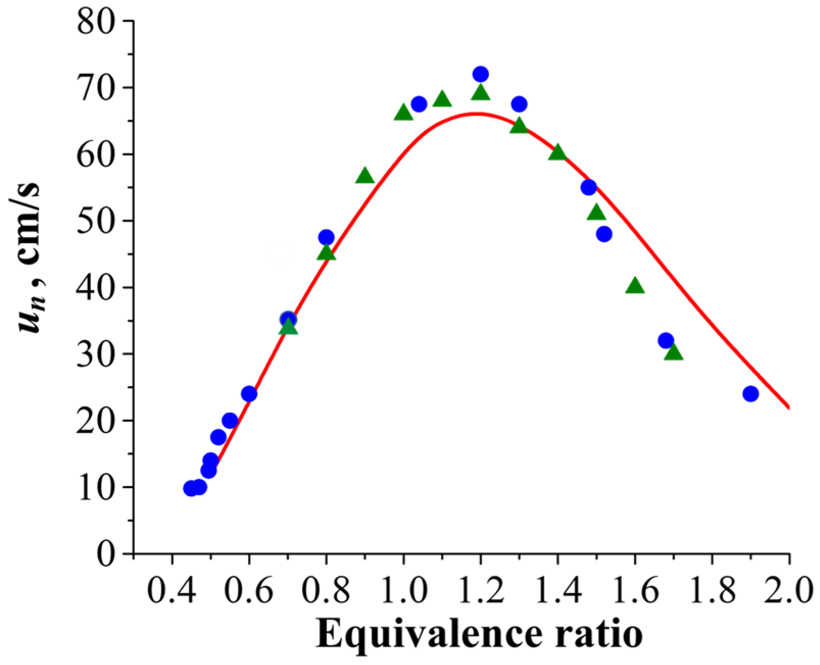
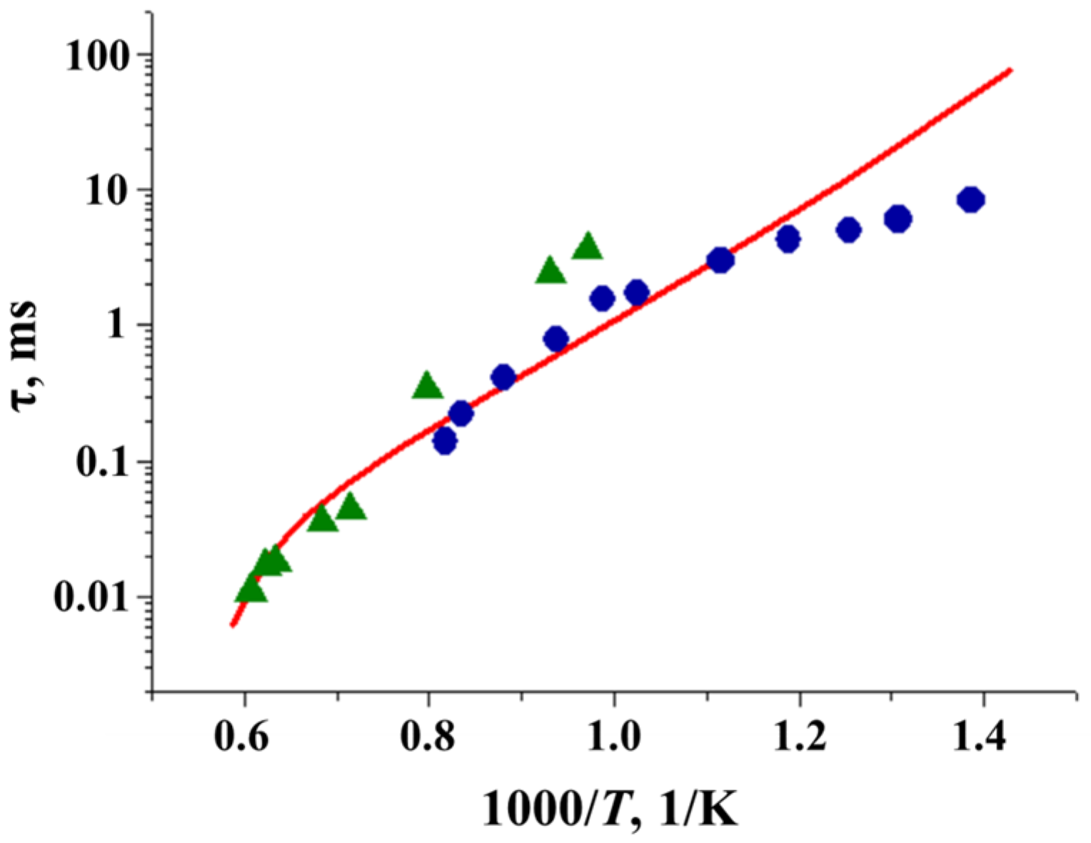
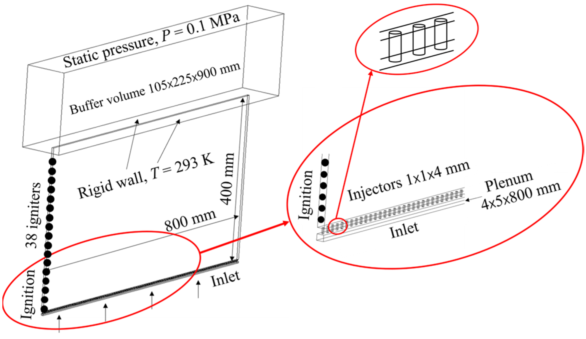
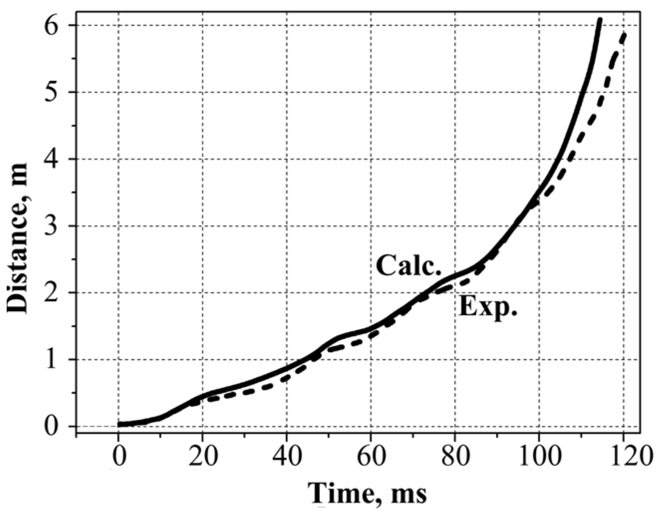
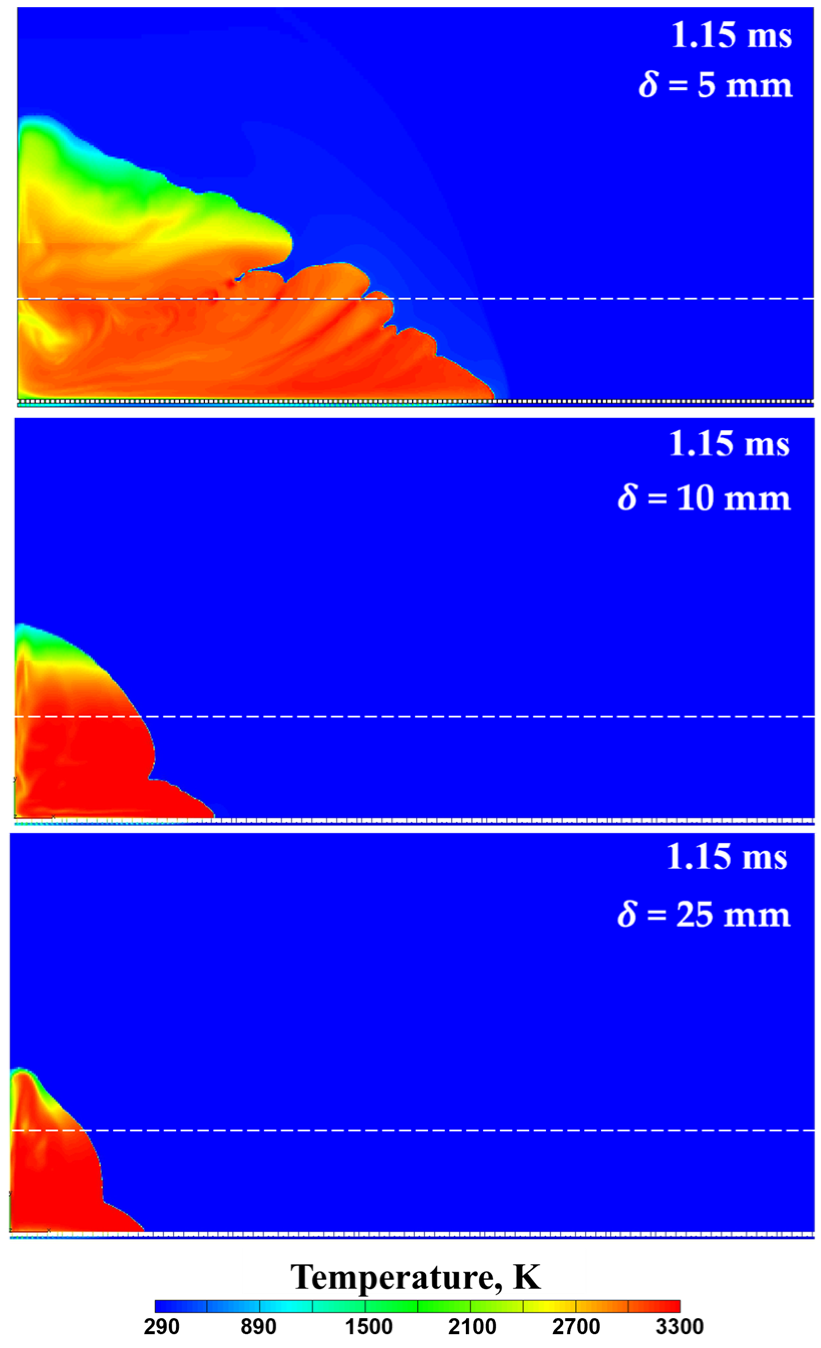
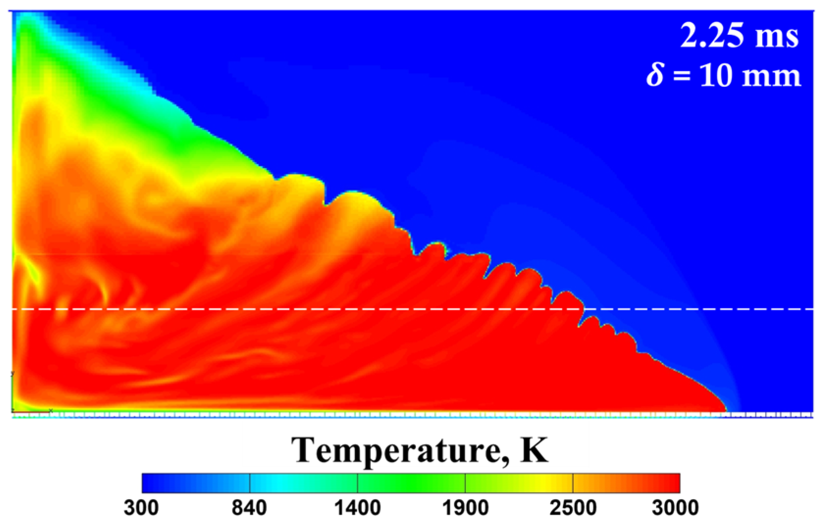
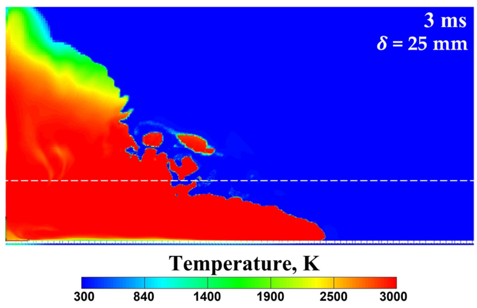
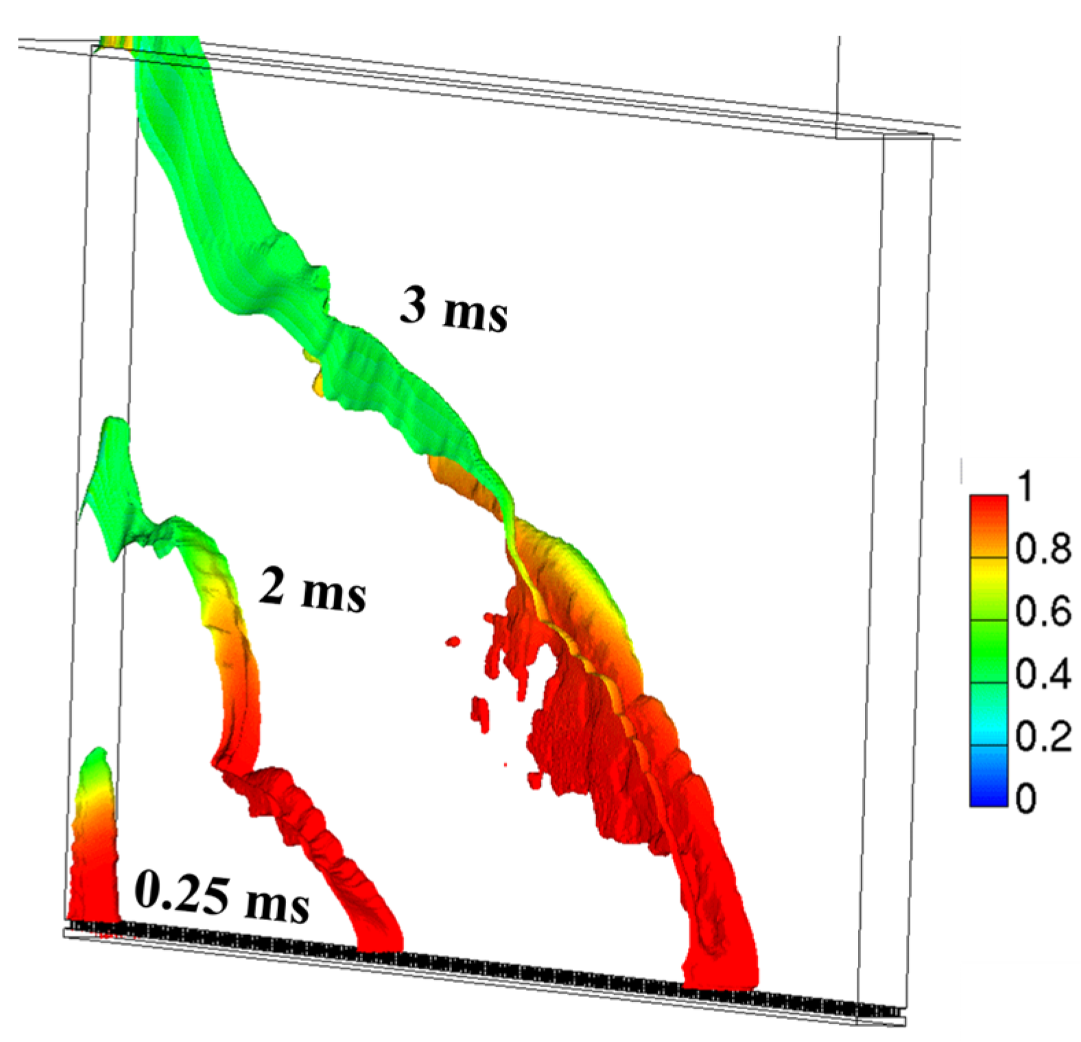
Table 1.
Volumetric oxidation of ethylene: Overall reaction mechanism.
| No. | Reaction | , (L, mol, s) | , kcal/mol |
|---|---|---|---|
| 1 | C2H4 + 2O2 → 2CO + 2H2O | 2∙108 | 25 |
| 2 | CO + H2O → CO2 + H2 | 1∙1012/ | 42 |
| 3 | CO2 + H2 → CO + H2O | 3.1∙1013/ | 50 |
| 4 | H2 + H2 + O2 → H2O + H2O | 7.0∙1013/ | 21 |
| 5 | CO + CO + O2 → CO2 + CO2 | 8.5∙1012/ | 21 |
Table 2.
Test conditions for calculations.
| Test No. | mm | vol.% | , L/min | , s | , mm | |
|---|---|---|---|---|---|---|
| 1 | 5 | 0 | 0 | 2.36 | 10 | 100 |
| 2 | 5 | 0 | 0 | 2.36 | 5 | 50 |
| 3 | 5 | 0 | 0 | 2.36 | 3 | 30 |
| 4 | 5 | 0.28 | 22 | 2.36 | 10 | 100 |
| 5 | 5 | 0.50 | 33 | 2.36 | 10 | 100 |
| 6 | 10 | 0 | 0 | 5.72 | 10 | 100 |
| 7 | 25 | 0 | 0 | 11.80 | 10 | 100 |
Disclaimer/Publisher’s Note: The statements, opinions and data contained in all publications are solely those of the individual author(s) and contributor(s) and not of MDPI and/or the editor(s). MDPI and/or the editor(s) disclaim responsibility for any injury to people or property resulting from any ideas, methods, instructions or products referred to in the content. |
© 2023 by the authors. Licensee MDPI, Basel, Switzerland. This article is an open access article distributed under the terms and conditions of the Creative Commons Attribution (CC BY) license (https://creativecommons.org/licenses/by/4.0/).
Share and Cite
MDPI and ACS Style
Ivanov, V.S.; Shamshin, I.O.; Frolov, S.M. Computational Study of Deflagration-to-Detonation Transition in a Semi-Confined Slit Combustor. Energies 2023, 16, 7028. https://doi.org/10.3390/en16207028
AMA Style
Ivanov VS, Shamshin IO, Frolov SM. Computational Study of Deflagration-to-Detonation Transition in a Semi-Confined Slit Combustor. Energies. 2023; 16(20):7028. https://doi.org/10.3390/en16207028
Chicago/Turabian StyleIvanov, Vladislav S., Igor O. Shamshin, and Sergey M. Frolov. 2023. "Computational Study of Deflagration-to-Detonation Transition in a Semi-Confined Slit Combustor" Energies 16, no. 20: 7028. https://doi.org/10.3390/en16207028
Note that from the first issue of 2016, this journal uses article numbers instead of page numbers. See further details here.