Estimating the Error of Fault Location on Overhead Power Lines by Emergency State Parameters Using an Analytical Technique

Abstract

Fault location on overhead power lines achieved with the highest possible accuracy can reduce the time to locate faults. This contributes to ensuring the stability of power systems, as well as the reliability of power supply to consumers. There are a number of known mathematical techniques based on different physical principles that are used in fault location on overhead power lines and whose errors vary. Fault location on overhead power lines uses techniques based on the estimation of emergency state parameters, which are referred to as distance-to-fault techniques and are widely used. They are employed in digital protection relay terminals and power-line fault locators. Factors that have a significant impact on the error of fault location on overhead power lines by emergency state parameters are design, manufacturing, and operation. The aim of this article is to analyze the existing techniques and to present a new analytical technique for estimating errors of fault location on overhead power lines by using emergency state parameters. The technique developed by the authors makes it possible to properly take into account a set of random factors, including various measurement errors of currents and voltages in the emergency state, which have a significant impact on the fault location on overhead power lines error. The technique allows one to determine more accurately the fault location and the size of the inspection area, which is necessary to reduce the time it takes to carry out emergency recovery operations. The proposed technique can be applied in fault locators and digital protection relay terminals that use both single-end, double- and multi-end sensing of currents and voltages in the emergency state.

1. Introduction

Fault location (FL) on overhead power lines (OPLs) that is as accurate as possible is one of the key operational tasks of electric utilities. The way it is addressed impacts the reliability of power system operation, including maintaining static and dynamic stability, as well as ensuring reliability of power supply to consumers [1,2,3]. Given an insufficient number of redundant OPLs, as well as devices for automatic switching of backup power in distribution grids, the issue of reducing the time for fault location and emergency recovery operations on OPLs is particularly relevant [4,5].

To solve the abovementioned problem, a number of mathematical techniques are used that are based on different physical principles that require information databases and calculations that vary in terms of their complexity [6]. Therefore, fault locators designed on their basis differ in terms of their error, which significantly affects the distance covered as part of the walk-around inspection of a OPL by technicians when searching for the actual fault location.

Of the FL techniques that are based on the estimation of emergency state parameters, the so called “distance-to-fault” [7,8,9] techniques are widely used. As a rule, they are implemented in the digital terminals of protection relays of OPLs or in stand-alone PL fault locators. The errors of the single-end, double- and multi-end OPL FL techniques are due to different causes. Most of the errors result from the OPL FL algorithm adopted, its features, and expressions used for calculations [10,11].

An analysis of methodological and random errors of OPL FL techniques includes the following:

• Determination of the parameters for calibrating the OPL fault locator based on specific parameters and configuration of the OPL;
• Calculation of parameters of currents and voltages in the assumed site of installation of the PL fault locator in case of faults at various points of the OPL;
• Identification of possible locations of OPL faults, using the selected OPL FL algorithm and the corresponding expressions used to perform calculations;
• Determination of the error of calculating the distance to the OPL fault location according to the chosen algorithm of the fault locator [12,13].

The regulatory and technical documents of electric utilities establish requirements for determining the OPL inspection area:

• ±15% of the OPL length, if its length is up to 50 km, inclusive;
• ±10% of the OPL length, if its length ranges from 50 to 100 km, inclusive;
• ±7% of the OPL length, if its length ranges from 100 to 300 km, inclusive;
• ±5% of the OPL length, if its length is 300 km or more [14].

Consequently, the maximum length of the OPL inspection area should not exceed the specified values. Technicians, after an emergency shutdown of the OPL with failed automatic reclosing, must arrange an inspection of the minimum possible section of the OPL, which depends on the accuracy of the adopted OPL FL algorithms [15,16].

An important feature of OPLs currently in operation is the non-uniformity of the resistivity along the OPL, which is due to the following:

• The use of different types of towers in individual sections of the OPL, which is due to, for example, the changes in the terrain of the OPL route;
• Changes in ground resistance at different sections of the OPL, which is caused by the route of the OPL running in areas with different types of soil (rocky, permafrost, swamps, floodplains of rivers, and reservoirs, etc.);
• Convergence at certain sections of a given OPL with other OPLs running within shared corridors;
• The absence of an overhead ground wire at some sections of the OPL (in some cases, by the design choice, the ground wire is used only on access routes to substations in regions with low lightning activity);
• Different lengths of OPL spans;
• Different types and cross-sections of wires on different sections of the OPL [17,18,19,20].

Therefore, failure to consider the above factors can lead to significant errors in calculating the distance to an OPL fault location.

Simulation tools are widely used nowadays to estimate the error of OPL FL algorithms [21,22,23]. In particular, the results of simulation make it possible to rule out the components of methodological errors in the calculation algorithm of the OPL FL, including those caused by non-uniformity of specific parameters of OPLs, thus significantly increasing the accuracy of calculating the distance to the fault location [22].

A large number of simulation results, as well as statistical data obtained from electric utilities, make the case for the expediency of applying statistical methods to estimate the errors of OPL FL techniques.

In [10], it was proposed to use a software package to implement statistical tests of OPL FL algorithms. The study found the conditional laws of distribution of errors of determining the distance to OPL fault location, while taking into account the probabilistic change in the parameters of the calculation algorithm. It was noted that the distribution of errors in calculating the distance to the OPL fault location was governed by the normal (Gaussian) law.

As a rule, electric utilities operating overhead OPLs do not have the capabilities to conduct simulations as well as advanced statistical data processing to calculate and analyze the errors of OPL FL techniques [24]. In this case, one should employ analytical techniques for estimating the errors of the OPL FL, which are significantly less computationally involved and hence allow performing approximate calculations “manually”.

The purpose of the article is to analyze the existing techniques of analytical estimation of OPL FL errors by emergency state parameters, as well as to present a novel technique developed by the authors.

2. Review of Techniques of OPL FL by Emergency State Parameters

Let us analyze the techniques of OPL FL based on measuring emergency state parameters [25].

One study [26] presented an OPL FL technique with asynchronous measurements from both of its ends, having a length (L), ohmic resistance, (R_PL), and inductive reactance (X_PL), connecting two power supply systems. This technique uses the results of measurements of instantaneous values of phase currents (i′_A, i′_B, i′_C), (i″_A, i″_B, i″_C) and voltages (u′_A, u′_B, u′_C), (u″_A, u″_B, u″_C) during a short circuit (SC) from the two ends of a OPL (′—the first end; ″—the second end). Based on these data, one determines the relative value of the distance to the SC location n and the physical distance from the end of the OPL having the index’ as per the expression L′ = n-L. When analyzing the waveforms of currents and voltages obtained from both ends of the OPL, they are aligned along the cut line at the moment of SC start; instantaneous values of currents i′ and i″ and voltages u′ and u″ of the faulty phase are measured; derivatives of current with respect to time di′/dt and di″/dt are calculated; and after that, the relative value of distance to fault location is determined as per Equation (1):

$$n=\frac{\left(u^{\prime }-u^{″}\right)+R_{\mathrm{PL}}{i}^{″}+X_{\mathrm{PL}}\frac{d{i}^{″}}{dt}}{R_{\mathrm{PL}}\left(i^{\prime }+i^{″}\right)+X_{\mathrm{PL}}\left(\frac{d{i}^{\prime }}{dt}+\frac{d{i}^{″}}{dt}\right)},$$

(1)

where n is the relative value of the distance to the SC location; u′ and u″ are instantaneous values of voltages obtained from waveforms of voltages of the faulty phase from the first and the second ends of the transmission line, V; i′ and i″ are instantaneous values of currents obtained from waveforms of currents of the faulty phase from the first and the second ends of the OPL, A; di′/dt and di″/dt are derivatives of currents with respect to time, A/s; and R_PL and X_PL are ohmic resistance and inductive reactance of OPL phases, Ohm.

The disadvantage of this technique is that no filtering is applied when processing instantaneous values of currents and voltages to reduce the effect of undesirable harmonic components and noise on the accuracy of the OPL FL. When power quality parameters (PQPs) deviate from standard values, the actual fault location on the OPL may be outside the PL walk-around inspection area. Moreover, this technique yields a large error on OPLs with non-uniform resistivity distribution along the line.

Another study [27] presented a technique for adapting the distance protection and OPL FL, which uses a mathematical model of the OPL. The technique uses data from measurements of fault currents and voltages and makes look-ahead iterative calculations with the OPL model by simulating faults at various points of the OPL. This calculates the difference in the distances between the simulated fault location and the one determined by the proposed OPL FL technique, on the basis of which the correction factors are calculated. The technique provides factoring in of the currents and voltages at the ends of OPLs obtained by the simulation not only during SCs at different points of the OPL but also in the case of various PQP deviations. PQP values are determined by the data from power-quality-control devices, based on which the correction factors are calculated to improve the accuracy of the OPL FL [28,29].

The downside of this technique is, arguably, the complexity of its implementation, as it requires a large number of computational experiments for each point of the short circuit in the OPL, with each having a different PQP deviation, calculations of correction factors, iterative calculations under different operating conditions of the OPL, storing in OPL fault locator a number of complex dependencies of OPL FL errors on various factors, etc. [30].

One study [31] considered a technique of OPL FL detection by using the data of measurements from its two ends, allowing the researchers to calculate the complex impedances of the forward (index 1), reverse (index 2), and zero (index 0) sequences, i.e., Z_1P L, Z_2 PL, and Z_0 PL. The calculations use data on the length of the OPL, L; measured values of complex phase currents (${{\dot{\mathrm{I}}}^{\prime }}_A$, ${{\dot{\mathrm{I}}}^{\prime }}_B$, and ${{\dot{\mathrm{I}}}^{\prime }}_C$), (${\dot{\mathrm{I}}}^{″}$_A, ${\dot{\mathrm{I}}}^{″}$_B, and ${\dot{\mathrm{I}}}^{″}$_C); and complex phase voltages (${\dot{\mathrm{U}}}^{\prime }$_A, ${\dot{\mathrm{U}}}^{\prime }$_B, and ${\dot{\mathrm{U}}}^{\prime }$_C), (${\dot{\mathrm{U}}}^{″}$_A, ${\dot{\mathrm{U}}}^{″}$_B, and ${\dot{\mathrm{U}}}^{″}$_C) of the main frequency at the moment of the SC from two line ends (’—the first end of the OPL; ”—the second end of the OPL), non-synchronized with respect to the angles. Based on these data, the calculation technique determines the type of SC, the relative value of the distance to the fault location (n), and the actual distance to the fault, L_SC = n·L. Furthermore, the angle between the corresponding voltages at the ends of the OPL is measured, for example, by means of GPS, and the vectors of currents and voltages at the second end are additionally rotated by the angle thus measured. This is necessary in order to convert phase currents and voltages into symmetrical components of complex forward, reverse, and zero sequence currents and voltages: (${\dot{\mathrm{I}}}^{\prime }$₁, ${\dot{\mathrm{I}}}^{\prime }$₂, and ${\dot{\mathrm{I}}}^{\prime }$₀), (${\dot{\mathrm{I}}}^{″}$₁, ${\dot{\mathrm{I}}}^{″}$₂, and ${\dot{\mathrm{I}}}^{″}$₀), (${\dot{\mathrm{U}}}^{\prime }$₁, ${\dot{\mathrm{U}}}^{\prime }$₂, and ${\dot{\mathrm{U}}}^{\prime }$₀), and (${\dot{\mathrm{U}}}^{″}$₁, ${\dot{\mathrm{U}}}^{″}$₂, and ${\dot{\mathrm{U}}}^{″}$₀). After that, the relative distances from the ends of the OPL to the fault location are determined by Equations (2) and (3): 

$$n_0^{\prime }=\frac{{\dot{U}}_0^{″}-{\dot{U}}_0^{\prime }+{\dot{I}}_0^{″}{\underset{\_}{Z}}_{0\mathrm{PL}}}{\left({\dot{I}}_0^{\prime }+{\dot{I}}_0^{″}\right){\underset{\_}{Z}}_{0\mathrm{PL}}},$$

(2)

$$n_0^{″}=\frac{{\dot{U}}_0^{\prime }-{\dot{U}}_0^{″}+{\dot{I}}_0^{\prime }{\underset{\_}{Z}}_{0\mathrm{OPL}}}{\left({\dot{I}}_0^{\prime }+{\dot{I}}_0^{″}\right){\underset{\_}{Z}}_{0L}}.$$

(3)

A significant shortcoming of this technique is the low accuracy of the OPL FL in the case of deviations of PQP from their standard values.

Another study [32] presented an OPL FL technique in which phase currents and voltages are measured at both ends of the OPL and are then converted into calculated complex values, using the expressions stated above. After that, using the imaginary parts of the calculated values, one calculates the relative and actual distances to the fault location from both ends of the OPL. The advantages of this technique include the fact that it does not use equivalent parameters of power supply systems and that there is no effect of the transient resistance in the OPL fault location.

The disadvantage of the technique is the need to use only imaginary components of the calculated values, which leads to an additional error in the OPL FL due to the insufficient amount of parameters taken into account.

Another study [33] presented an OPL FL technique in which the need to use only imaginary components of the calculated values was eliminated. For this purpose, the angle between the currents at the ends of the OPL was measured by using digital communication channels or a Global Positioning System (GPS). In the first case, the angles are determined on the basis of time-synchronized samples, or by continuously calculating the time of signal passage between the two sub-assemblies of the differential protection of the OPL. In the second case, time synchronization pulses are received from GPS signal receivers. Next, phase currents and voltages are measured at both ends of the OPL, converted into calculated complex values as per the expressions stated above, and, using the complete calculated values, one finds the relative and actual distances to the fault location from both ends of the OPL. The advantages of the technique are that it does not rely on equivalent parameters of the power supply systems, and it eliminates the effect of the transient resistance at the point of the OPL fault.

The disadvantage of the technique is the need to use sophisticated equipment and algorithms, such as digital communication channels between the ends of OPLs, as well as satellite time-synchronization equipment.

Each of the considered techniques of OPL FL by emergency state parameters has its error, the value of which depends both on the errors of the parameters included in the calculation expressions used in calculating the distance to the fault location and a variety of external factors.

3. Techniques of Estimating the Error of OPL FL Based on the Errors of the Parameters Included in the Expression for Calculating the Distance to the Fault Location

The key factors that have a significant impact on the OPL FL error can be provisionally divided into three groups: design, production, and operation [10].

The design factor is due to the methodological error of the adopted OPL FL technique, arising at the stage of design of a OPL fault locator, for example, due to the impossibility of accounting or compensating for variables that affect the results of the calculation of the distance to the fault location.

The production factor is related to the specifications of an OPL fault locator and its proper condition.

The operation factor is due to errors in setting the parameters of the OPL and/or power supply systems, as well as to errors in transmitting data, such as emergency state waveforms, to power-line technicians.

In general, depending on the availability and accuracy of the necessary input data for the implementation of an OPL FL technique, the time of its execution may vary [34]. The actual time of restoring the power supply to consumers who do not have a backup power supply and who are powered from a faulty OPL depends on this [35,36,37]. Power-line technicians cannot be sent out to carry out emergency recovery operations on the OPL until the calculation has not been performed and the distance to the fault in relation to one of the supplying substations has not been determined. Both the location of the walk-around inspection area and its length depend on the accuracy of calculation results.

If the calculation is implemented so as to yield large errors, the period of time to locate the fault on the OPL will be considerable—in the extreme case, lasting up to the moment when the fault is detected by visual examination. Taking into account the location of places for entry of specialized equipment onto OPLs, the presence of hard-to-access areas due to natural (rivers, swamps, mountains, etc.) and manmade (protected areas of enterprises, special industrial facilities, etc.) factors, the time required for a walk-around inspection OPLs depends in a complex way on the magnitude of the OPL FL error and is unique to each OPL and its sections [38,39].

In [27], it was noted that the calculation of the distance to the fault location (x_f) of the OPL by emergency state parameters (ESPs) is determined by a functional relationship of the following form:

$$x_f=F\left(I_1,I_2,U_1,U_2,Z_{\mathrm{SI}1},Z_{\mathrm{MI}2},Z_{\mathrm{PL}},L\dots \right),$$

(4)

where $I_1,I_2$ and $U_1,U_2$ are the currents and voltages at the ends of the OPL; $Z_{c1} \mathrm{and} Z_{c2}$ are the matrices of self impedances and mutual impedances of adjoining power systems; $Z_{\mathrm{PL}}$ is the matrix of complex impedances of OPLs; and L is the length of the OPL.

If currents and voltages are not measured at both ends of the OPL, and the OPL has one or more branches or intermediate cables, then the relationship (4) will become significantly more complicated, and, in many cases, it will not have an unambiguous solution.

It is important to note that calculation expressions similar to (4) are formed by the designers of OPL fault locators under the assumption that the conditions of absolute symmetry and pure sine wave of currents and voltages corresponding to the industrial frequency of 50 Hz hold true for the PL. In the case of a violation of the spatial coherence of current and voltage signals during double-end or multi-end OPL FL, as caused, for example, by PQP deviation, there will be additional errors in the calculations of the distance to the fault that are not taken into account as part of the analytical calculations [40]. Thus, each OPL FL algorithm has its specific resilience to violations of the spatial coherence of currents and voltages, as well as the specific dependency of errors in calculations of distances to the fault location on the calculation expression used.

On the basis of the adopted OPL FL technique, operating conditions, and parameters of the OPL, a calculation expression corresponding to (4) is formed, which includes the values used in calculations of the distance to the fault location. For Equation (4), there is also a relationship of the error of calculating the distance to the fault, which has the following form:

$$\Delta x_f=F\left(\Delta I_1,\Delta I_2,\Delta U_1,\Delta U_2,\Delta Z_{\mathrm{SI}1},\Delta Z_{\mathrm{MI}2},\Delta Z_{\mathrm{PL}},\Delta L\dots \right),$$

(5)

where $\Delta I_1,\Delta I_2,\Delta U_1,\Delta U_2,\Delta Z_{\mathrm{SI}1},\Delta Z_{\mathrm{MI}2},\Delta Z_{\mathrm{PL}},\Delta L\dots$ are errors of measurement of currents, voltages, resistances, and power line length involved in the calculation.

When estimating the total error of the OPL FL$, \Delta x_f$, it is advisable to use statistical methods [13,27], and the ways they are used when solving the problem may vary.

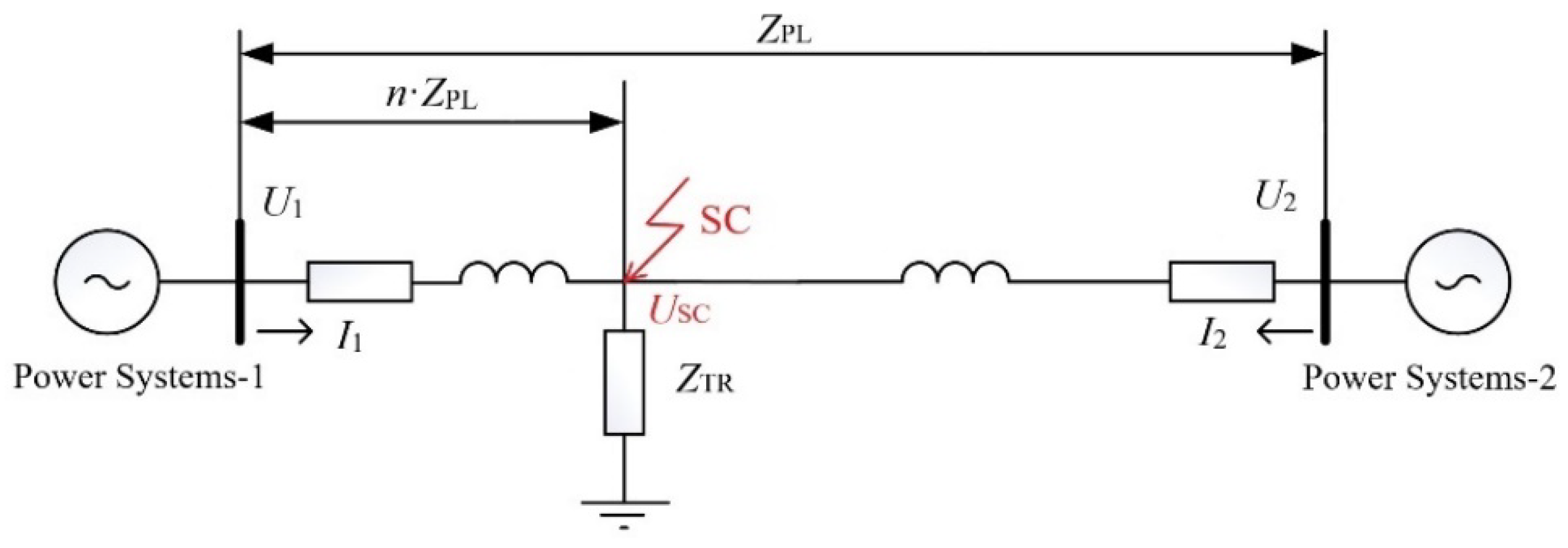
One study [27] proposed a technique based on the assertion that the OPL FL is an indirect measurement procedure, and the total error, $\Delta x_f$, is the sum of the estimation errors of each of the parameters involved in the calculation of Equation (4). Therefore, the final expression for determining the OPL FL error takes the form of an expression for determining the total RMS value. Let us clarify the procedure for performing analytical calculations through a case study of an OPL during a short-circuit through transient resistance, Z_TR, as shown in Figure 1.

The main calculation expressions of the OPL FL technique are formed on the basis of the results of measurements of current and voltage moduli at the ends of the OPL I₁, I₂, U₁, and U₂, as well as the following expressions:

$$I_1·n·Z_{\mathrm{PL}}+U_1=U_{\mathrm{SC}},$$

(6)

$$I_2\left(1-n\right) Z_{\mathrm{PL}}+U_2=U_{\mathrm{SC}}.$$

(7)

Given that the distance to the fault location (the SC point) is equal to$x_f=n·L$, and equating Equations (6) and (7), after transformations, we arrive at the following expression:

$$x_f=\frac{U_2-U_1+I_2·L·Z_{\mathrm{PL}}}{\left(I_1+I_2\right)Z_{\mathrm{PL}}}.$$

(8)

The application of the calculation of Equation (8) in PL fault locators is characterized by the following features [27]:

• The Equation (8) is valid for components of both reverse and zero sequences, and the OPL FL procedure is implemented by making constant the corresponding moduli of currents $I_1 \mathrm{and} I_2$and voltages $U_1 \mathrm{and} U_2$, which greatly simplifies the engineering solution;
• When performing OPL FL, it is not necessary to know the type of the short circuit (single-phase or two-phase);
• Transient resistance at the fault location is not used in the calculations, since the double-end measurement virtually eliminates its effect on the error of the OPL FL technique;
• Since the calculation is performed using the components of the reverse and zero sequences, which are absent in the loaded state, the influence of the value of the load on the accuracy of the OPL FL technique is completely ruled out;
• Calculation algorithm is simple enough, in terms of its software/hardware implementation in OPL fault locators or digital relay protection terminals [41,42].

Let us consider an example of the implementation of the OPL FL technique for a real-world 220 kV OPL, with a length of L = 120 km, based on the actual measurements obtained for one of the emergency states during a short circuit in the OPL. We perform the calculation as per Equation (8) by the components of the zero sequence, and Z_l = Z₀ = 3·0.426 = 1.278 Ohm/km. The amplitudes of the currents and voltages at the ends of the OPL measured by the digital relay protection terminals are as follows: I₁ = 2.0 kA, I₂ = 0.56 kA, U₁ = 40 kV, and U₂ = 28 kV [27].

We then calculate the distance to the fault on the OPL:

$$x_f=\frac{U_2-U_1+I_2·L·Z_{\mathrm{PL}}}{\left(I_1+I_2\right)Z_{\mathrm{PL}}}=\frac{28-40+0.56·120·1.278}{\left(2.0+0.56\right)·1.278}=22.582 \left(\mathrm{km}\right).$$

(9)

Based on the assumptions made, the error of the indirect measurement of x_f for the example under consideration corresponds to the following expression:

$$\Delta x_f=\sqrt{{\left(\frac{\partial x_f}{\partial I_1}\Delta I_1\right)}^2+{\left(\frac{\partial x_f}{\partial I_2}\Delta I_2\right)}^2+{\left(\frac{\partial x_f}{\partial U_1}\Delta U_1\right)}^2+{\left(\frac{\partial x_f}{\partial U_2}\Delta U_2\right)}^2+{\left(\frac{\partial x_f}{\partial Z_0}\Delta Z_0\right)}^2+{\left(\frac{\partial x_f}{\partial L}\Delta L\right)}^2}.$$

(10)

Taking into account the partial derivatives calculated (Equation (10)), as well as error values set, ∆I₁ = 10%, ∆I₂ = 5%, ∆U₁ = ∆U₂ = 3%, ∆Z₀ = 5%, and ∆L = 2%, for the given example, the OPL FL is attained with the following accuracy [27]:

$$x_f=22.582\pm \Delta x_f=22.582\pm 2.08 \left(\mathrm{km}\right).$$

(11)

It is important to note that the OPL FL techniques, which use calculation expressions, directly depend on the power-line topology and its parameters, and this is one of their main drawbacks. Increasing the complexity of the calculation algorithm and expanding the number of parameters involved, so as to minimize the error of the OPL FL, leads to an increase in the computational load on the OPL fault locator and introduces additional dependence on the amount and accuracy of the data used in the calculation [22].

3.1. Error Analysis Using the Parameters of the PL FL Error Distribution

An overwhelming majority of the OPL FL algorithms, when calculating the distance to the fault, x_f, are based on calculating the ratio of scalar quantities of the following form [43]:

$$x_f=\frac{y_1}{y_2}.$$

(12)

If y₁ and y₂ are calculated without errors, that is, there are no measurement errors of currents and voltages in the emergency state and no distorting factors, then the OPL FL is implemented with the required accuracy. However, in the presence of random factors (interference, noise, etc.), the situation drastically changes for the worse.

Suppose that y₁ and y₂ are random variables governed by the normal distribution laws y₁$\in$N(m₁, σ₁) and y₂$\in$N(m₂, σ₂), where m and σ are the expected value (mathematical expectation) and standard deviation for the normal (Gaussian) distribution of a random variable with the probability density:

$$p_y=\frac{1}{\sigma \sqrt{2\pi }}{e}^{\left(\frac{-{\left(y-m\right)}^2}{2{\sigma }^2}\right)}.$$

(13)

If the variances of the quantities y₁ and y₂ are small, an approximate expression can be accepted for practical OPL FL calculations:

$$x_f\approx \frac{m_1}{m_2}.$$

(14)

However, in the case of nonzero variance values, the quantities y₁ and y₂, calculations that rely on the approximate Equation (14) will lead to large OPL FL errors, which are unacceptable in the context of real-world operation.

Another study [43] proposed to use statistical characteristics of the quantity to obtain analytical estimates of OPL FL errors:

$$yy=1/y, \mathrm{where} y \in N(m,\sigma )$$

(15)

This determines the expected value M[yy] of the quantity yy, for which the distribution (15) is valid. In [42], it was proposed to use the following expression:

$$M\left[\mathrm{yy}\right] \approx 1/m,\mathrm{for}\sigma <<m,$$

(16)

as well as the inequality

M[yy(y)] > yy(M[y]),

(17)

for the convex function yy of the stochastic variable y.

Note that the convexity of the function yy is ensured at y > 0, so the inequality (17) cannot be applied directly to analytical calculations.

To calculate the expected value of the variable 1/y, we use the following expression:

$$M\left[\frac{1}{y}\right]={{\displaystyle \int }}_{-\infty }^{\infty }\frac{1}{y}{p}_y\left(y\right)dy={{\displaystyle \int }}_{-\infty }^{\infty }\frac{1}{y}·\frac{1}{\sigma \sqrt{2\pi }}{e}^{\left(\frac{-{\left(y-m\right)}^2}{2{\sigma }^2}\right)}dy.$$

(18)

In order to perform calculations using Expression (18), it is necessary to implement numerical integration. However, in the case of infinite limits, this integral has a discontinuity point at y = 0. To solve (18), study [43] proposed special mathematical techniques for obtaining the finite distribution of the expected value:

$$M\left[\frac{1}{y}\right]=\frac{1}{\sigma }{e}^{\frac{-m^2}{2{\sigma }^2}}{{\displaystyle \int }}_0^{\raisebox{1ex}{$m$}\!\left/ \!\raisebox{-1ex}{$\sigma $}\right.}\frac{1}{y}{e}^{\frac{y^2}{2}}dy.$$

(19)

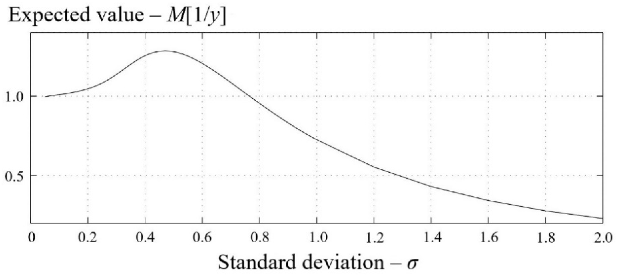
The integral of the Equation (19) is continuous and has limited integration limits, so it allows us to solve a number of practical problems of estimating the OPL FL error. In particular, given that m is normalized, we can plot the dependency of the expected value of the calculated distance to the fault location—M [1/y] as a function of the standard deviation σ of the variable y (Figure 2). The probabilistic variable y has a normal distribution with the expected value m = 1 and standard deviation, σ.

Our analysis of Figure 2 allows us to draw the following conclusions:

• The expected value of the quantity (1/m) tends toward 1/m and is equal to one only when σ$\to 0$;
• If the RMS value of σ reaches large values, then the expected value of the variable (1/y) tends toward zero. This phenomenon is explained by the fact that the distribution (normalized Gaussian probability density) of the variable y is symmetric with respect to zero;
• An increase in the variance (standard deviation σ) leads to an even greater tendency of M[1/y] toward zero;
• For small values of σ (σ = 0.1, …, 0.75), we obtain estimates of the expected value M[1/y] that exceed unity. This indicates a bias in the OPL FL estimates for this group of techniques;
• To ensure the high accuracy of the OPL FL by ESP, it is extremely important to reduce the variance of the variable y or to compensate for the biases of the OPL FL estimates by applying adaptation techniques [22].

Another study [43] noted challenges arising in estimating the error variance of the OPL FL by ESP. These challenges are caused by difficulties in solving the following integral expression:

$$M\left[\frac{1}{y^2}\right]={{\displaystyle \int }}_{-\infty }^{\infty }\left(\frac{1}{y^2}\right)p_y\left(y\right)dy={{\displaystyle \int }}_{-\infty }^{\infty }\left(\frac{1}{y^2}\right)\left(\frac{1}{\sigma \sqrt{2\pi }}\right)e^{\frac{-{\left(y-m\right)}^2}{2{\sigma }^2}}dy.$$

(20)

An in-depth mathematical analysis notwithstanding, the author of [43], unfortunately, did not propose practically significant techniques for calculating the errors of OPL FL techniques, and there are no calculations of errors for specific examples of faults in OPLs.

In those cases where it is not possible to obtain exact value of the numerical characteristics of random variables, it is advisable to use approximate expressions. The authors of the article are not aware of other methods for the analytical evaluation of potential errors of fault location on overhead power lines.

3.2. Approximate Calculation of the Expected Value and Variance in Determining the Distance to the Fault on the OPL

Let us assume that the previously introduced value, x (x_f is the distance to the location of the short circuit in the OPL), has a relatively small variance σ²(x). Such an assumption is valid because it makes no practical sense to use OPL FL techniques with large errors in calculating the distance to the fault location.

Let η = α(x), where α(x) is a sufficiently smooth function. Note that, under the introduced constraints, there is an approximate expression for the mean value of M[η] = M[α(x)] that has a small error.

Let us use Taylor’s formula:

$$\alpha \left(x\right)=\alpha \left(a\right)+{\alpha }^{\prime }\left(a\right)\left(x-a\right)+\left(\frac{{\alpha }^{″}\left(a\right)}{2}\right){\left(x-a\right)}^2+\left(\frac{{\alpha }^{‴}{x}_1}{6}\right){\left(x-a\right)}^3; (a\gtrless x_1 \gtrless x).$$

(21)

By replacing a with M[x], we obtain the following:

$$\alpha \left(x\right)=\alpha \left(M\left[x\right]\right)+{\alpha }^{\prime }\left(M\left[x\right]\right)x^o+{\alpha }^{″}\left(\frac{M\left[x\right]}{2}\right){\left(x^o\right)}^2+\left(\frac{{\alpha }^{‴}}{6}\right)x_1{\left(x^o\right)}^3; (M[x] \gtrless x_1 \gtrless x).$$

(22)

Since the variance σ²(x) is assumed to be small, the fluctuation, x^o, takes mostly small absolute values. Therefore, the last term in the right-hand side of Equation (22) turns out to be significantly smaller than all the others. By neglecting it, we obtain the approximate formula:

$$\alpha \left(x\right)\approx \alpha \left(M\left[x\right]\right)+{\alpha }^{\prime }\left(M\left[x\right]\right)x^o+\left(\frac{{\alpha }^{″}M\left[x\right]}{2}\right){\left(x^o\right)}^2,$$

(23)

from which it follows that

$$M\left[\alpha \left(x\right)\right]\approx \alpha \left(M\left[x\right]\right)+{\alpha }^{\prime }\left(M\left[x\right]\right)M\left[x^o\right]+{\alpha }^{″}\left(\frac{M\left[x\right]}{2}\right)M{\left[x^o\right]}^2.$$

(24)

Since M[x^o] = 0, we arrive at the approximate formula for the expected value:

$$M\left[\alpha \left(x\right)\right]\approx \alpha \left(M\left[x\right]\right)+{\alpha }^{″}\left(\frac{M\left[x\right]}{2}\right){\sigma }^2\left(x\right).$$

(25)

By reasoning in a similar way, we can show that if f(X) = α(x₁, x₂, …, x_n) = α(X) is a sufficiently smooth function of n variables x₁, x₂, …, x_n, and the vector projections y₁, y₂, …, y_n are pairwise uncorrelated (in particular, independent) random variables, then the general expression for the expected value will take the following form:

$$M\left[\alpha \left(y\right)\right]\approx \alpha \left(M\left[y\right]\right)+\frac{1}{2}{{\displaystyle \sum }}_{i=1}^n{{\alpha }^{″}}_{xi,xi}\left(M\left[y\right]\right){\sigma }^2\left(y_i\right).$$

(26)

In the case of the OPL FL problem in question, we have the following:

$$x_f\left(y_1,y_2\right)=\frac{y_1}{y_2},$$

(27)

where y₁ and y₂ are independent random variables with small variances, and M[y₂] is non-zero; then we have α(y₁, y₂) = y₁/y₂. Hence, we obtain the following:

$$\alpha \left(x_1,x_2\right)=\frac{x_1}{x_2}, {{\alpha }^{″}}_{x1, x1}\left(x_1,x_2\right)=\frac{2x_1}{x_2^3}, {{\alpha }^{″}}_{x2, x2}\left(x_1,x_2\right)=0.$$

(28)

Thus, taking into account the Equation (26), we obtain an approximate formula for calculating the expected value in determining the fault location on the OPL:

$$M\left[x_f\right]=M\left[\frac{y_1}{y_2}\right]\approx \frac{M\left[y_1\right]}{M\left[y_2\right]}+\frac{M\left[y_1\right]{\sigma }^2\left(y_2\right)}{{\left(M\left[y_2\right]\right)}^3}$$

(29)

We use the approximate Equations (24) and (25) to approximate the variance of techniques for OPL FL by ESPs of the forms (4) and (27). By subtracting the second expression from the first and discarding the terms containing (x^o)² and σ²(x) = M[x^o]², we obtain the following:

$${\eta }^o=\eta -M\left[\eta \right]=\alpha \left(x\right)-M\left[\alpha \left(x\right)\right]={\alpha }^{\prime }M\left[\alpha \left(x\right)\right]x^o.$$

(30)

Therefore, ${\left({\eta }^o\right)}^2\approx {\left[{\alpha }^{\prime }\left(M\left[x\right]\right)\right]}^2{\left(x^o\right)}^2$; hence, we obtain the following:

$${\sigma }^2\left[\alpha \left(x\right)\right]={\sigma }^2\left(\eta \right)=M{\left({\eta }^o\right)}^2\approx {\left[{\alpha }^{\prime }\left(M\left[x\right]\right)\right]}^2{\sigma }^2\left(x\right).$$

(31)

Thus, the variance can be calculated by the following expression:

$${\sigma }^2\left[\alpha \left(x\right)\right]\approx {\left[{\alpha }^{\prime }\left(M\left[x\right]\right)\right]}^2{\sigma }^2\left(x\right).$$

(32)

Generalizing Equation (32) to the case of a random vector function, when vector projections y₁, y₂, …, y_n are pairwise uncorrelated (in particular, independent) random variables, we arrive at the following expression:

$${\sigma }^2\left[\alpha \left(y\right)\right]\approx {{\displaystyle \sum }}_{i=1}^n{\left[{{\alpha }^{\prime }}_{xi}\left(M\left[y\right]\right)\right]}^2{\sigma }^2\left(y_i\right).$$

(33)

When applied to the case of the OPL FL problem in question, we obtain the following:

$$x_f\left(y_1,y_2\right)=\frac{y_1}{y_2},$$

(34)

where y₁ and y₂ are independent random variables with small variances, and M[y₂] is non-zero; then we have α(y₁, y₂) = y₁/y₂.

Since

$$\alpha \left(x\right)=\alpha \left(x_1, x_2\right)=\frac{x_1}{x_2}, \mathrm{that} {\alpha }^{\prime }{}_{x1}\left(x_1,x_2\right)=\frac{-x_1}{x_2^2}, {{\alpha }^{\prime }}_{x2}\left(x_1,x_2\right)=\frac{1}{x_2},$$

(35)

then, taking into account Equation (33), we obtain an approximate formula for calculating the variance of the error of the OPL FL by emergency state parameters:

$${\sigma }^2\left(x_f\right)={\sigma }^2\left(\frac{y_1}{y_2}\right)\approx {\sigma }^2\left(y_2\right)\left(\frac{{\left(M\left[y_1\right]\right)}^2}{{\left(M\left[y_2\right]\right)}^2}\right)+\frac{{\sigma }^2\left(y_1\right)}{{\left(M\left[y_2\right]\right)}^2}$$

(36)

3.3. Results of Statistical Analytical Calculations of PL FL Errors

Using the results of the calculations obtained earlier, let us determine the statistical characteristics of the OPL FL errors by using approximate Equations (29) and (36).

First, for the calculation relation (29), we obtain analytically the statistical characteristics of the numerator and denominator corresponding to the random variables y₁ and y₂ (Equation (4)). We assume that the random variables involved in calculating the OPL FL are uncorrelated and centered. In calculations, let us assume that the measurement error of random variables corresponds to their RMS value; for example, ∆L = σ_L [44,45,46].

Given that

$$y_1=U_2-U_1+I_2·L·Z_{\mathrm{PL}} ; y_2=\left(I_1+I_2\right)Z_{\mathrm{PL}},$$

(37)

the expected values of the random variables y₁ and y₂ will be determined by the measured values [27]:

$$M\left(y_1\right)=y_1=28-40+0.56·120·1.278=73.882 \left(\mathrm{kV}\right),$$

$$M\left(y_2\right)=y_2=\left(2.0+0.56\right)·1.278=3.272\left(\mathrm{kV}\right)$$

We obtain the following expressions for the variances σ²(y₁) and σ²(y₂):

$${\sigma }^2\left(y_1\right)={\sigma }^2\left(U_2\right)– {\sigma }^2\left(U_1\right)+{\sigma }^2\left(I_2\right)·{\sigma }^2\left(L·Z_{\mathrm{PL}}\right)+{\left(M\left(I_2\right)\right)}^2{\sigma }^2\left(L·Z_{\mathrm{PL}}\right)+$$

$${\left(M\left(L·Z_{\mathrm{PL}}\right)\right)}^2{\sigma }^2\left(I_2\right)={\sigma }^2\left(U_2\right)-{\sigma }^2\left(U_1\right)+\left[{\left(M\left(I_2\right)\right)}^2+{\sigma }^2\left(I_2\right)\right]·$$

$$\left[{\sigma }^2\left(L\right)·{\sigma }^2\left(Z_{\mathrm{PL}}\right)+{\left(M\left(L\right)\right)}^2·{\sigma }^2\left(Z_{\mathrm{PL}}\right)+{\left(M\left(Z_{\mathrm{PL}}\right)\right)}^2{\sigma }^2\left(L\right)\right]+{\left(M\left(L\right)\right)}^2{\left(M\left(Z_{\mathrm{PL}}\right)\right)}^2{\sigma }^2\left(I_2\right);$$

(38)

$${\sigma }^2\left(y_2\right)=\left[{\sigma }^2\left(I_1\right){\sigma }^2\left(Z_{\mathrm{PL}}\right)+{\left(M\left(I_1\right)\right)}^2·{\sigma }^2\left(Z_{\mathrm{PL}}\right)+{\left(M\left(Z_{\mathrm{PL}}\right)\right)}^2·{\sigma }^2\left(I_1\right)\right]+$$

$$+\left[{\sigma }^2\left(I_2\right){\sigma }^2\left(Z_{\mathrm{PL}}\right)+{\left(M\left(I_2\right)\right)}^2{\sigma }^2\left(Z_{\mathrm{PL}}\right)+{\left(M\left(Z_{\mathrm{PL}}\right)\right)}^2{\sigma }^2\left(I_2\right)\right]={\sigma }^2\left(Z_{\mathrm{PL}}\right)[{\sigma }^2\left(I_1\right)+{\left(M\left(I_1\right)\right)}^2+$$

$$+{\sigma }^2\left(I_2\right)+{\left(M\left(I_2\right)\right)}^2\left]+{\left(M\left(Z_{\mathrm{PL}}\right)\right)}^2·\right[{\sigma }^2\left(I_1\right)+{\sigma }^2\left(I_2\right)].$$

(39)

Numerical values of the variables included in Equations (38) and (39) are summarized in

Table 1. Variables for analytical calculation of OPL FL errors.

RMS Values
Variable	σ(U1) (kV)/%	σ(U2) (kV)/%	σ(I1) (kA)/%	σ(I2) (kA)/%	σ(L) (km)/%	σ(ZPL) (Ohm/km)/%
Value	1.2/3	0.84/3	0.2/10	0.028/5	2.4/2	0.0639/5
Expected Values
Variable	M(I1) (kA)	M(I2) (kA)		M(L) (km)		M(ZPL) (Ohm/km)
Value	2.0	0.56		120		1.278

.

Substitution of numerical values (Table 1) in relationships (38) and (39) leads to the following results:

$${\sigma }^2\left(y_1\right)={\sigma }^2\left(U_2\right)-{\sigma }^2\left(U_1\right)+\left[{\left(M\left(I_2\right)\right)}^2+{\sigma }^2\left(I_2\right)\right]·$$

$$\left[\left({\sigma }^2\left(L\right)\right){\sigma }^2\left(Z_{\mathrm{PL}}\right)+{\left(M\left(L\right)\right)}^2{\sigma }^2\left(Z_{\mathrm{PL}}\right)+{\left(M\left(Z_{\mathrm{PL}}\right)\right)}^2{\sigma }^2\left(L\right)] \right]+{\left(M\left(L\right)\right)}^2{\left(M\left(Z_{\mathrm{PL}}\right)\right)}^2{\sigma }^2\left(I_2\right)=$$

$$\begin{gathered} ={\left(0.84\right)}^2-{\left(1.2\right)}^2+\left[{\left(0.56\right)}^2+{\left(0.028\right)}^2\right]·\left[{\left(2.4\right)}^2·{\left(0.0639\right)}^{2 }+{\left(120\right)}^2· {\left(0.0639\right)}^2+{\left(1.278\right)}^2·{\left(2.4\right)}^2\right] \\ +{\left(120\right)}^2·{\left(1.278\right)}^2·{\left(0.028\right)}^2=39.155 {\left(\mathrm{kV}\right)}^2, \end{gathered}$$

(40)

$${\sigma }^2\left(y_2\right)={\sigma }^2\left(Z_{\mathrm{PL}}\right)\left[{\sigma }^2\left(I_1\right)+{\left(M\left(I_1\right)\right)}^2+{\sigma }^2\left(I_2\right)+{\left(M\left(I_2\right)\right)}^2\right]+$$

$$+{\left(M\left(Z_{\mathrm{PL}}\right)\right)}^2·\left[{\sigma }^2\left(I_1\right)+{\sigma }^2\left(I_2\right)\right]={\left(0.0639\right)}^2·\left[{\left(0.2\right)}^2+{\left(2.0\right)}^2+{\left(0.028\right)}^2+{\left(0.56\right)}^2\right]+$$

$$+{\left(1.278\right)}^2·\left[{\left(0.2\right)}^2+{\left(0.028\right)}^2\right]=0.0844{\left(\frac{\mathrm{kV}}{\mathrm{km}}\right)}^2.$$

(41)

Then the variance of the OPL FL error according to expressions (36), (40), and (41) and calculations of M(y₁) and M(y₂) will be as follows:

$${\sigma }^2\left(x_f\right)={\sigma }^2\left(y_2\right)·\frac{{\left(M\left[y_1\right]\right)}^2}{{\left(M\left[y_2\right]\right)}^2}+\frac{{\sigma }^2\left(y_1\right) }{{\left(M\left[y_2\right]\right)}^2}=$$

$$=0.0844\frac{{\left(73.882\right)}^2}{{\left(3.272\right)}^2}+\frac{39.155}{{\left(3.272\right)}^2}=46.689 \left({\mathrm{km}}^2\right)$$

(42)

To solve the practical problems of the OPL FL, it is advisable to calculate the distance to the fault location not by the Equation (4), but by the relationship (29), which takes the following numerical value:

$$M\left[x_f\right]=\frac{M\left[y_1\right]}{M\left[y_2\right]}+\frac{ M\left[y_1\right]{\sigma }^2\left(y_2\right)}{{\left(M\left[y_2\right]\right)}^3 }=\frac{73.882 }{3.272}+\frac{73.882·0.0844 }{{\left(3.272\right)}^3}=22.758 \left(\mathrm{km}\right).$$

(43)

Turning to the form of Equation (11), we obtain the following:

$$x_f=M\left[x_f\right] \pm \sigma \left(x_f\right)=22.758 \pm 6.83 \left(\mathrm{km}\right).$$

(44)

Consequently, the probability of finding a fault in an OPL within the area defined by Equation (44), given the normal distribution law and specified statistical parameters of the random variables shown in Table 1, will be 68.27%.

4. Discussion of the Proposed Analytical Technique for Estimating the Error of OPL FL by ESP

Our analysis of the results obtained by Equations (38)–(44) allows us to draw the following conclusions:

• Compared to the analytical calculation by Equations (9)–(11), which assume the use of partial derivatives, Equations (38)–(44) involve weighted sums of statistical variables (expected values and variances). The presented analytical technique allows us to take into account in a more comprehensive way the totality of random factors that have a significant impact on the error of the OPL FL based on the parameters of the emergency state;
• If the calculation of the distance to the fault location is a function of a ratio of random variables of the form x_f = y₁/y₂, then, from a statistical point of view, it is necessary to use the expected value M[x_f] (Equation (43)) of this ratio to carry out OPL FL. The use of the specified calculation value allows one to take into account various measurement errors of currents and voltages in the emergency state in the most proper way possible. This case is common because current and voltage measuring transformers of different kinds and types, with different specifications and accuracy classes, are usually installed at the ends of the same OPL;
• Our analysis of calculation Equations (38)–(44), which serve as the basis of a new analytical technique for estimating the errors of the OPL FL by emergency state parameters, shows that they are valid for single-end, as well as double-end and multi-end, OPL FL techniques;
• The obtained calculation expressions for the expected value and variance of the distance to the fault of the OPL allow us to calculate, with greater accuracy, the distance to the fault, as well as the size of the inspection area, which is critical for power-line technicians.

5. Conclusions

The potential accuracy of calculating the distance to the fault location by emergency state parameters has significant differences for each specific OPL. It depends on statistical data on errors of current and voltage measuring transformers, specific features of digital processing of current and voltage signals in the PL fault locator, and accuracy of specifying the values of parameters of the OPL being analyzed and their actual values, as well as a number of other factors.

The presented analytical technique for assessing the error of the OPL FL by emergency state parameters makes it possible to determine the fault location and the size of the inspection area with greater accuracy, which is necessary to reduce the time it takes to perform emergency recovery operations, in order to ensure the stability of power systems and the reliability of power supply to consumers.

The proposed mathematical expressions are of much practical importance, because they can be adopted in the OPL fault locators and digital relay protection terminals that use single-end, as well as double- and multi-end, sensing of currents and voltages while in the emergency state.

References

- Ghadi, M.; Rajabi, A.; Ghavidel, S.; Azizivahed, A.; Li, L.; Zhang, J. From active distribution systems to decentralized microgrids: A review on regulations and planning approaches based on operational factors. Appl. Energy 2019, 253, 113543. [Google Scholar] [CrossRef]
- Schwan, M.; Ettinger, A.; Gunaltay, S. Probabilistic reliability assessment in distribution network master plan development and in distribution automation implementation. In Proceedings of the CIGRE, 2012 Session, Paris, France, 26–30 August 2012; p. C4-203. [Google Scholar]
- Alberto Escalera, A.; Prodanović, M.; Castronuovo, E.D. Analytical methodology for reliability assessment of distribution networks with energy storage in islanded and emergency-tie restoration modes. Int. J. Electr. Power Energy Syst. 2019, 107, 735–744. [Google Scholar] [CrossRef]
- Lebedev, V.; Filatova, G.; Timofeev, A. Increase of accuracy of the fault location methods for overhead electrical power lines. Adv. Mater. Sci. Eng. 2018, 2018, 3098107. [Google Scholar] [CrossRef]
- Lebedev, V.D.; Yablokov, A.A.; Filatova, G.A.; Lebedeva, N.V.; Petrov, A.E. Development and research of fault location algorithm for double-end feed lines in the multifunctional system. In Proceedings of the 2019 2nd International Youth Scientific and Technical Conference on Relay Protection and Automation (RPA 2019), Moscow, Russia, 24–25 October 2019; p. 8958174. [Google Scholar]
- Kulikov, A.L.; Obalin, M.D. The development of software to support decision-making in the elimination of damage on power transmission lines. Izv. High. Educ. Institutions. Electromech. 2015, 2, 70–75. (In Russian) [Google Scholar]
- Saha, M.M.; Izykowski, J.; Rosolowski, E. Fault Location on Power Networks; Springer: London, UK, 2010; p. 437. [Google Scholar]
- Shalyt, G.M.; Eisenfeld, A.I.; Maly, A.S. Determination of Places of Damage to Power Transmission Lines According to the Parameters of the Emergency Mode; Energoatomizdat: Moscow, Russia, 1983; p. 208. (In Russian) [Google Scholar]
- Schweitzer, E.O. A review of impedance-based fault locating experience. In Proceedings of the 14th Annual Iowa–Nebraska System Protection Seminar, Omaha, NE, USA, 16 October 1990; pp. 1–31. [Google Scholar]
- Arzhannikov, E.A.; Lukoyanov, V.Y.; Misrikhanov, M.S. Determining the Location of a Short Circuit on High−Voltage Power Transmission Lines; Shuin, V.A., Ed.; Energoatomizdat: Moscow, Russia, 2003; p. 272. (In Russian) [Google Scholar]
- Artsishevsky, Y.L. Determination of the Places of Damage to Power Transmission Lines in Networks with Grounded Neutral; Higher School: Moscow, Russia, 1988; p. 94. (In Russian) [Google Scholar]
- Minullin, R.G. Detecting the faults of overhead electric-power lines by the location-probing method. Russ. Electr. Eng. 2017, 88, 61–70. [Google Scholar] [CrossRef]
- Kulikov, A.L. Digital Remote Detection of Power Line Damage; Misrikhanov, M.S., Ed.; Publishing House of the Volga-Vyatka Academy of State: Nizhniy Novgorod, Russia, 2006; p. 315. (In Russian) [Google Scholar]
- СТО 56947007-29.240.55.224-2016; Guidelines for Determining the Places of Damage to Overhead Lines with a Voltage of 110 kV and Higher (Date of Introduction: 17.08.2016). PJSC FGC UES: Moscow, Russia, 2016. (In Russian)
- Ilyushin, P.V. Emergency and post-emergency control in the formation of micro-grids. E3S Web Conf. 2017, 25, 02002. [Google Scholar] [CrossRef]
- Ilyushin, P.V.; Filippov, S.P. Under-frequency load shedding strategies for power districts with distributed generation. In Proceedings of the 2019 International Conference on Industrial Engineering, Applications and Manufacturing (ICIEAM), Sochi, Russia, 25–29 March 2019. [Google Scholar] [CrossRef]
- Kosyakov, A.A.; Kuleshov, P.V.; Pogudin, A.L. The influence of the grounding device structure of a substation on the voltage of conducted interference of lightning currents. Russ. Electr. Eng. 2019, 90, 752–755. [Google Scholar] [CrossRef]
- Shevchenko, N.Y.; Ugarov, G.G.; Kirillova, S.N.; Lebedeva, Y.V. Review and analysis of the design features of overhead power line wires with increased resistance to icy-wind loads. Quest. Electr. Technol. 2018, 4, 53–63. (In Russian) [Google Scholar]
- Sharipov, U.B.; Égamnazarov, G.A. Calculating currents in lightning protection cables and in optical cables built into them during asymmetric short circuits in overhead transmission lines. Power Technol. Eng. 2017, 50, 673–678. [Google Scholar] [CrossRef]
- Voitovich, P.A.; Lavrov, Y.A.; Petrova, N.F. Innovative technical solutions for the construction of ultra-compact high-voltage overhead power transmission lines. New Russ. Electr. Power Ind. 2018, 8, 44–57. (In Russian) [Google Scholar]
- Senderovich, G.A.; Zaporozhets, A.O.; Gryb, O.G.; Karpaliuk, I.T.; Shvets, S.V.; Samoilenko, I.A. Automation of determining the location of damage of overhead power lines. In Control of Overhead Power Lines with Unmanned Aerial Vehicles (UAVs); Sokol, Y.I., Zaporozhets, A.O., Eds.; Studies in Systems, Decision and Control; Springer: Cham, Switzerland, 2021; Volume 359, pp. 35–53. [Google Scholar]
- Obalin, M.D.; Kulikov, A.L. Application of adaptive procedures in algorithms for determining the location of damage to power lines. Ind. Power Eng. 2013, 12, 35–39. (In Russian) [Google Scholar]
- Senderovich, G.A.; Zaporozhets, A.O.; Gryb, O.G.; Karpaliuk, I.T.; Shvets, S.V.; Samoilenko, I.A. Experimental studies of the method for determining location of damage of overhead power lines in the operation mode. In Control of Overhead Power Lines with Unmanned Aerial Vehicles (UAVs); Sokol, Y.I., Zaporozhets, A.O., Eds.; Studies in Systems, Decision and Control; Springer: Cham, Switzerland, 2021; Volume 359, pp. 55–77. [Google Scholar]
- Suslov, K.; Shushpanov, I.; Buryanina, N.; Ilyushin, P. Flexible power distribution networks: New opportunities and applications. In Proceedings of the 9th International Conference on Smart Cities and Green ICT Systems (SMARTGREENS), Prague, Czech Republic, 2–4 May 2020; pp. 57–64. [Google Scholar] [CrossRef]
- Izykowski, J. Fault Location on Power Transmission Line; Springer: London, UK, 2008; p. 221. [Google Scholar]
- Visyashchev, A.N. Devices and Methods for Determining the Location of Damage on Power Transmission Lines: A Textbook. At 2 h. h. 1; Publishing House of ISTU: Irkutsk, Russia, 2001; p. 188. (In Russian) [Google Scholar]
- Belyakov, Y.S. Actual issues of determining the places of damage to overhead power lines. Electr. Eng. Libr. 2010, 11, 1–80. (In Russian) [Google Scholar]
- Suslov, K.V.; Solonina, N.N.; Smirnov, A.S. Distributed power quality monitoring. In Proceedings of the IEEE 16th International Conference on Harmonics and Quality of Power (ICHQP), Bucharest, Romania, 25–28 May 2014; pp. 517–520. [Google Scholar]
- Gallego, L.; Torres, H.; Pavas, A.; Urrutia, D.; Cajamarca, G.; Rondón, D. A Methodological proposal for monitoring, ana-lyzing and estimating power quality indices: The case of Bogotá–Colombia. In Proceedings of the IEEE Power Tech 2005, Saint Petersburg, Russia, 27–30 June 2005. [Google Scholar]
- Ilyushin, P.V.; Shepovalova, O.V.; Filippov, S.P.; Nekrasov, A.A. Calculating the sequence of stationary modes in power distribution networks of Russia for wide-scale integration of renewable energy based installations. Energy Rep. 2021, 7, 308–327. [Google Scholar] [CrossRef]
- Minullin, R.G.; Akhmetova, I.G.; Kasimov, V.A.; Piunov, A.A. Location monitoring with determination of damage location and current operability of overhead power transmission lines. Electr. Station 2022, 11, 30–38. (In Russian) [Google Scholar]
- Suslov, K.; Solonina, N.; Solonina, Z.; Akhmetshin, A. Development of the method of determining the location of a short circuit in transmission lines. J. Phys. Conf. Ser. 2021, 2061, 012033. [Google Scholar] [CrossRef]
- Kulikov, Y.A. The technology of vector registration of parameters and its application to control the modes of the UES of Russia. Electro. Electr. Eng. Electr. Power Ind. Electr. Ind. 2011, 2, 2–5. (In Russian) [Google Scholar]
- Izykowski, J. Location of complex faults on overhead power line. Prz. Elektrotechniczny 2016, 7, 81–84. [Google Scholar] [CrossRef]
- Byk, F.L.; Myshkina, L.S.; Khokhlova, K. Power supply reliability indexes. In Proceedings of the International Conference on Actual Issues of Mechanical Engineering, Tomsk, Russia, 27–29 July 2017; pp. 525–530. [Google Scholar]
- Filippov, S.P.; Dilman, M.D.; Ilyushin, P.V. Distributed Generation of Electricity and Sustainable Regional Growth. Therm. Eng. 2019, 66, 869–880. [Google Scholar] [CrossRef]
- Ilyushin, P.; Filippov, S.; Kulikov, A.; Suslov, K.; Karamov, D. Specific Features of Operation of Distributed Generation Facilities Based on Gas Reciprocating Units in Internal Power Systems of Industrial Entities. Machines 2022, 10, 693. [Google Scholar] [CrossRef]
- Ahmedova, O.; Soshinov, A.; Shevchenko, N. Analysis of influence of external atmospheric factors on the accuracy of fault location on overhead power lines. In Proceedings of the E3S Web of Conferences, Proceedings of the High Speed Turbomachines and Electrical Drives Conference 2020 (HSTED-2020), Prague, Czech Republic, 14–15 May 2020; EDP Sciences: Les Ulis, France, 2020; Volume 178, p. 01057. [Google Scholar]
- Margitová, A.; Kolcun, M.; Kanálik, M. Impact of the Ground on the Series Impedance of Overhead Power Lines. Trans. Electr. Eng. 2018, 7, 47–54. [Google Scholar] [CrossRef]
- Rylov, A.; Ilyushin, P.; Kulikov, A.; Suslov, K. Testing Photovoltaic Power Plants for Participation in General Primary Frequency Control under Various Topology and Operating Conditions. Energies 2021, 14, 5179. [Google Scholar] [CrossRef]
- Kulikov, A.P.; Sharygin, M.V.; Ilyushin, P.V. Principles of organization of relay protection in microgrids with distributed power generation sources. Power Technol. Eng. 2020, 53, 611–617. [Google Scholar] [CrossRef]
- Dong, A.H.; Geng, X.L.; Yang, Y.; Su, Y.; Li, M.Y. Overhead Power Line Fault Positioning System. Appl. Mech. Mater. 2013, 329, 299–303. [Google Scholar] [CrossRef]
- Akke, M. Some Control Applications in Electric Power System. Ph.D. Thesis, Lund University, Lund, Sweden, 1997. [Google Scholar]
- Suloeva, E.S.; Romantsova, N.V. Mathematical and software for determining the error in the modeling of the measuring instrument. Model. Optim. Inf. Technol. 2021, 9, 4. [Google Scholar]
- Qian, H.; Qiu, Z.; Wu, Y. Robust extended Kalman filtering for nonlinear stochastic systems with random sensor delays, packet dropouts and correlated noises. Aerosp. Sci. Technol. 2017, 66, 249–261. [Google Scholar] [CrossRef]
- Liu, Y.; Shen, B.; Zhang, P. Synchronization and state estimation for discrete-time coupled delayed complex-valued neural networks with random system parameters. Neural Netw. 2022, 150, 181–193. [Google Scholar] [PubMed]
Figure 1.
Simplified single-line diagram of PL in case of a short circuit through transient resistance.
Figure 2.
The dependency of the expected value of the quantity (1/y) on σ.