
Impact of Geometry on a Thermal-Energy Storage Finned Tube during the Discharging Process

1
Department of Electrical, Electronics and Computer Engineering (DIEEI), University of Catania, 95125 Catania, Italy
2
Italian National Research Council, Institute for Advanced Energy Technologies “Nicola Giordano” (CNR-ITAE), 98126 Messina, Italy
*
Author to whom correspondence should be addressed.
Energies 2022, 15(21), 7950; https://doi.org/10.3390/en15217950
Submission received: 20 September 2022
/
Revised: 21 October 2022
/
Accepted: 23 October 2022
/
Published: 26 October 2022
(This article belongs to the Topic Advances in Solar Heating and Cooling)
Abstract
:This work focused on the modelling of latent heat thermal energy storage systems. The mathematical modelling of a melting and solidification process has time-dependent boundary conditions because the interface between solid and liquid phases is a moving boundary. The heat transfer analysis needs the interface position over time to predict the temperature inside the liquid and the solid regions. This work started by solving the classical two-phase (one-dimensional) Stefan problem through a Matlab implementation of the analytical model. The same physical problem was numerically simulated using ANSYS FLUENT, and the good match of analytical and numerical results validated the numerical model, which was used for a more interesting problem: comparing three different latent heat TES configurations during the discharging process to evaluate the most efficient in terms of maximum average discharging power. The three axial heat conduction structures changed only for the fin shape (rectangular, trapezoidal and fractal), keeping constant the volume fractions of steel, aluminium and PCM to perform a proper comparison. Results showed that the trapezoidal fin profile performs better than the rectangular one, and the fractal fin profile geometry was revealed as the best for faster thermal exchange when the solidifying frontier moves away from the steel ring. In conclusion, the average discharging power for the three configurations was evaluated for a time corresponding to a reference value (10%) of the liquid fraction: the rectangular fin profile provided 950.8 W, the trapezoidal fin profile 979.4 W and the fractal fin profile 1136.6 W, confirming its higher performance compared with the other two geometries.
1. Introduction
One of the most pressing challenges of modern society is energy transition. Environmental degradation and the increase in the world population are responsible for the effort to develop new green solutions in recent days. The key strategy seems to be using renewable energy, initially in combination with fossil fuels, with the goal of covering 100% of energy generation by the year 2050 [1].
Some forms of renewable energy, such as wind or sunlight, fluctuate over time and geography [2], so it is not easy to realize efficient long-term energy storage [3]. Thus far, there has been a lack of location-independent, cost-effective storage on a power-plant scale. Still, it is believed that energy storage systems (ESS) will play a relevant role in achieving energy systems based on renewable energy sources (RES). Worldwide, researchers are working on solutions to this topic to develop cost-effective, virtually lossless ESS able to absorb and release large amounts of electrical energy.
Today, the well-known pumped hydro energy storage (PHES) systems and electrochemical batteries are the main electrical-energy storage technologies, but there are more technical and economical constraints that hinder their development. Furthermore, the former technology, even if already mature and widely used [4], is usually limited by geological constraints. Katsaprakakis et al. [5] investigated PHES application and other electricity storage technologies in three autonomous Greek islands and concluded that PHES system can be feasible for small islands under favorable land morphology. From an economic point of view, the case study in the island of Rhodes, presented by Arnaoutakis et al. in [6], has not very attractive economic indices.
Compressed-air-energy storage (CAES) systems suffer geographical restrictions too, and environmental concerns [4].
Large-scale compressed-hydrogen storage is a promising green solution for energy storage in balancing intermittent renewable electricity production. Elberry et al. [7] discussed different compressed hydrogen storage technologies such as storage vessels, geological storage and other underground storage alternatives, concluding that a techno-economic chain analysis is needed to establish which storage option is more suitable for a specific case. Another energy storage solution (power-to-fuel) stores surplus energy as synthetic fuel, such as methanol. Methanol can be produced as a net carbon-neutral fuel from green hydrogen and captured CO2. Synthetic fuels are easy to store and do not require significant infrastructure investment.
Storage options also include thermal-based solutions, the power-to-heat-to-power storage systems: surplus electricity is used to generate high-temperature heat that charges a thermal-energy storage (TES) system; the stored heat can be reconverted when electricity is required (the discharging process) through a thermal power cycle. In general, thermal system efficiency is limited by Carnot efficiency, which defines the maximum roundtrip efficiency (typically 40% for real systems) [4]. However, in a Carnot battery concept variant, called a pumped thermal-energy storage (PTES) system, heat is pumped by a heat pump, and able to deliver much more than one unit of heat per unit of electrical energy consumed. This allows the efficiency to be no longer limited by the Carnot efficiency, and a PTES system can ideally reach roundtrip efficiency (calculated as the ratio of the electrical energy generated during the discharging process to the electrical energy consumed during the charging process) of up to 100% [8].
Furthermore, a PTES system can receive thermal integration from low-temperature heat sources, for example, waste heat from industrial processes. In this case, the compression work during the charging process can be reduced and the efficiency (calculated as the ratio of the electrical energy generated during the discharging process to the electrical energy consumed during the charging process with an integrated heat source) might, thereby, exceed 100% [9].
Thermal-energy storage systems can be used to store surplus energy provided by renewable sources power plants, such as wind parks [10] and CSP (concentrated solar power) plants [11,12]. They have been successfully applied worldwide in very different applications, such as the Hofmühl Brewery in Eichstatt (Germany) [13,14], the RESlag project (Spain) [15,16], the Andasol Solar Power Station (Spain) [17] and the CHESTER project (Germany) [18,19]. Molten salt TES can also be used for high-temperature industrial-process heating. A modular, scalable system concept is under development by the Norwegian company Kyoto Group [20].
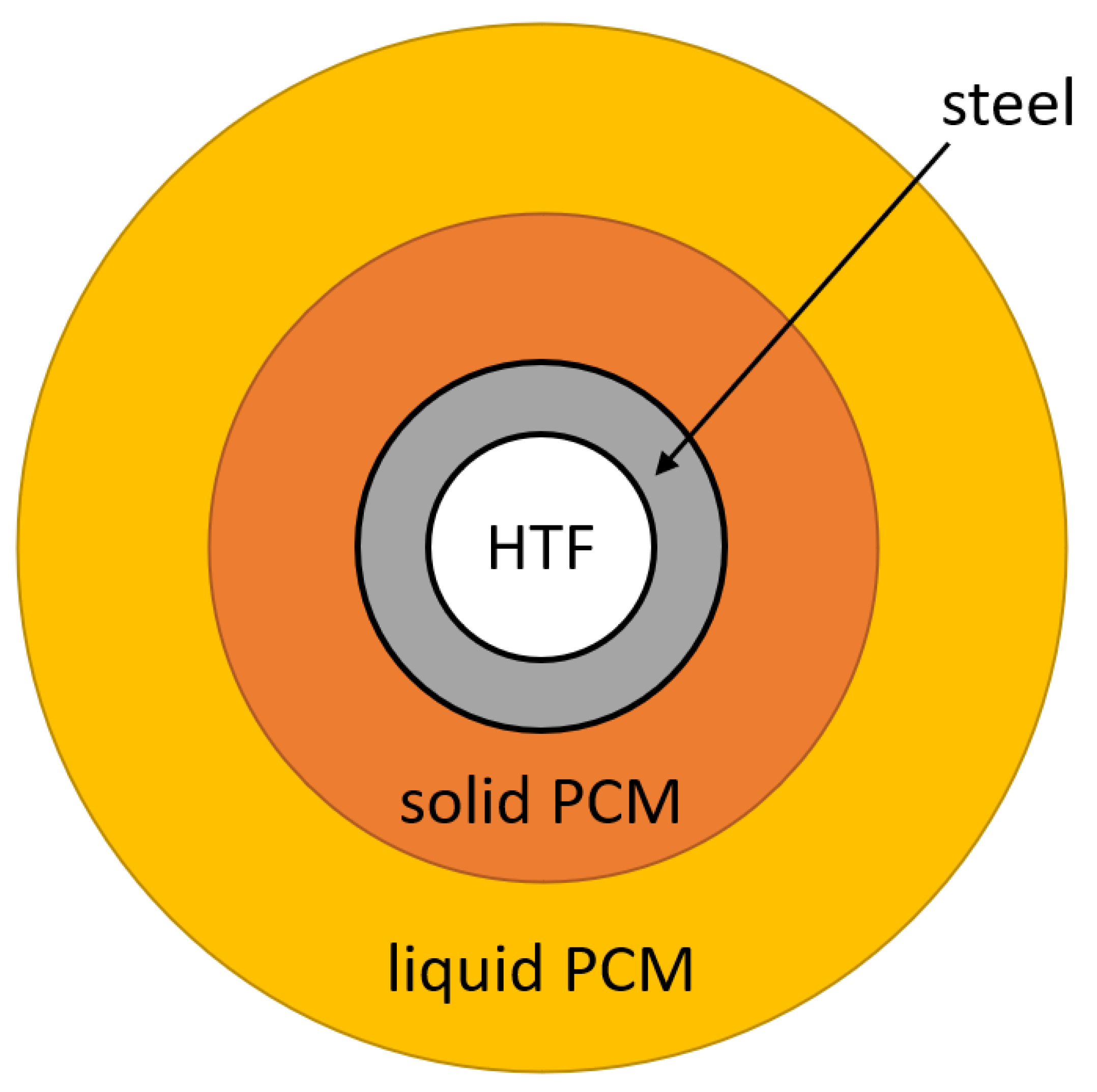
Among thermal-energy storage solutions, this work investigated the latent heat alternative. Latent-heat thermal-energy storage uses the physical state change in the storage medium when storing or releasing thermal energy. In most applications, the phase transition is from solid to liquid or liquid to solid. Phase change materials are relatively inexpensive, but they must be accurately selected for every application [21,22,23] on the basis of very different metrics, such as energy density, cost and operating temperature [24]. Their main disadvantage is low thermal conductivity. For example, the thermal conductivity of sodium nitrate (NaNO3) is /( ). In comparison, low-alloy steel (e.g., an evaporator tube made of 16Mo3) has about 80 times higher thermal conductivity. Low thermal conductivity significantly affects the performance of latent heat storage: during the discharging process (Figure 1), the PCM begins to solidify and a solid layer forms around the pipe (in general, heat transfer in solid materials is lower than in the liquid due to the lack of convection); as the discharge continues, the solid layer increases in thickness, further increasing the thermal resistance. Consequently, the heat flow decreases asymptotically, the discharging power becomes very small and the discharging time unusably long. A latent-heat storage system cannot operate in this condition, especially with small driving temperature differences.
To increase the performance of latent heat storage, many solutions have been identified over last years, aiming to reduce melting and solidification times. This goal can be achieved in two different ways:
- 1.
- By improving the thermal conductivity of the PCM mass;
- 2.
- By increasing the contact area between the exchanger structure and the PCM mass.
The first solution increases thermal conductivity by adding more conductive additives, such as metal matrices [23], metal foams or metal rings. Their use significantly improves thermal conductivity, but they occupy a relatively large volume inside the PCM melt, reducing the storage capacity. Furthermore, they have a non-constant thermal conduction path because there is no defined connection from the evaporator tube to the metal structures. These structures are relatively expensive to manufacture and unsuitable for large-scale use [25].
Further improvements can be made by adding metal dust or carbon-fiber structures [26]. These have some disadvantages: PCM and added materials segregate due to differences in density; and the melting temperature can change with metal dust additions. When using carbon fibers, thermal-conductivity improvement is highly dependent on the spatial arrangement of the fibers. The use of these methods for large-scale industrial production is also unsuitable.
The second solution aims to increase the contact area between PCM mass and the heat conducting structure by encapsulating PCM inside a metal shell or using thermally conductive structures.
Encapsulation significantly increases the heat exchange surface. However, the manufacturing process is complex and, therefore, expensive. In addition, encapsulation must be able to manage the thermal expansion of the PCM. For example, the volumetric expansion of NaNO3 upon melting is 10.7% [27]. Furthermore, an operating medium is required to heat exchange between PCM and HTF if HTF is water: direct water evaporation on the encapsulated PCM requires the storage to be designed and built as a pressure vessel of appropriate size.
A more promising technique is PCM microencapsulation, which increases heat transfer area, reduces PCM reactivity towards the outside environment and prevents PCM from leaking when it is in the liquid state. Microencapsulation is a process that allows for enclosing solid, droplet, liquid or gaseous PCM in a compatible thin solid wall. The material inside the MEPCM (microencapsulated phase change material) is called “core” and the wall is named “shell”. Microencapsulation fabrication methods can generally be categorized into chemical, physico-chemical and physico-mechanical processes [28]. Dong et al. [29] proposed an optimized fabrication method for an MEPCM. A Gallium ingot, used as a PCM, was mixed in a high-speed mixer to form Ga droplets. Then, Ga droplets were added to distilled water in a heated PTFE container. The hydrothermal treatment continued with filtration and drying in order to obtain a precursor shell of GaOOH. Finally, the GaOOH MEPCM was calcined under an oxygen gas flow to form a stable Ga2O3 MEPCM using a thermogravimetry device. Tests on MEPCM showed that the high rate of the heat storage capacity of the raw material was retained after encapsulation, preserving good stability in heat storage after many thermal cycles. Microencapsulation is expected to establish a new foundation for heat storage in the high-temperature region [30,31].
Another good solution to the heat conduction problem is using heat conduction structures connected to the heat transfer tube. They can generally be divided into radial and axial structures. In the first case, the thermal conduction structure consists of many plates arranged transversely to the heat transfer fluid (HTF) pipe at a constant distance. The axial heat conduction structures are arranged along the longitudinal direction of the HTF pipe.
Comparison carried out in [32] showed that, during the melting process, the axial fins were more efficient, enabling free convection, while free convection was largely suppressed in the radial fins. During the solidification process, only heat conduction played a role since the free convection can be ten times lower than in the melting process [33].
Axial fins offer much more design flexibility. They can be unbranched, mono-branched, doubly branched and various other shapes, manufactured (by extrusion) more cost-effectively than the radial structures. Design flexibility causes different PCM volume contents and surface configurations, making it difficult to compare the performance of the structures. For this reason, it is not easy to establish which structure is more efficient and economically more convenient.
Numerical analyses can help to evaluate the performance of different configurations. In this optic, this study had the purpose of comparing three axial heat conduction structures to evaluate the most efficient in terms of maximum average discharging power. The three configurations have different fin shapes but the same radial dimensions to avoid different volume contents in metal and phase change material which would make a proper comparison difficult.
The paper is organized as follows: Section 2 explains how to mathematically model a solidification and melting problem, describing the analytical model and the Newmann solution for the classical two-phase (one-dimensional) Stefan problem, which is analytically solved through Matlab; in Section 3, the same physical problem is numerically simulated using ANSYS FLUENT 2021 R1; the comparison of analytical and numerical results is reported in Section 4 for the validation of the numerical model. Then, Section 5 compares three axial heat conduction structures with different fin shapes to evaluate the most efficient in terms of maximum average discharging power. Finally, Section 6 summarizes the results, and proposes future research activities.
2. Mathematical Modelling of Solidification and Melting Processes
The mathematical modelling of a phase change process aims to find the temperature field in the modeled material (with all the other heat transfer features), when the position over time of the moving frontier that separates the existing phases is known.
During a melting or solidification process, the domain will be subdivided into liquid and solid regions, separated by an interface. The enthalpy of phase change is absorbed (melting) or released (freezing) on the solid/liquid interface, so the moving interface characterizes the phase change process. Such problems have time-dependent boundary conditions and are known as “moving boundary problems” or “free boundary problems”. Very few explicit analytical solutions are available for such problems in the literature. Their analysis requires knowing the initial temperature distribution and the thermal conditions on every exterior surface of the solid and liquid part of the body, also in the moving boundary, to have a well-posed mathematical problem.
The interface is the moving boundary of both the liquid and solid regions, and the following conditions are needed to complete the initial-boundary value problem [34]:
where is the temperature depending on space and time, and is the melting temperature.
The heat conduction equation is satisfied in each region, but a further condition (the interface position over time) is required to predict the temperature inside the liquid and the solid phases, as shown from the boundary limits in Equations (1) and (2). This condition results from a heat balance across the interface and is known as the “Stefan condition”.
2.1. Analytical Solution of the Classical Two-Phase (One-Dimensional) Stefan Problem
Stefan formulated the mathematical problem of finding the temperature field of a melting slab together with its solid/liquid interface history, determined as part of the solution [34]. The classical Stefan problem is considered the prototype of all phase-change models, even if the closed-form explicit solutions (of similarity type) need the following simplifying assumptions: a one-dimensional and semi-infinite geometry, thermophysical properties constant in each region, a constant melting temperature and enthalpy of phase change, a constant density in all the domains, a uniform initial temperature, a constant wall temperature, no internal heating source in the material, a zero-thickness sharp interface and heat transferring isotropically by conduction only (ignoring convection yields a conservative estimate of the melting speed).
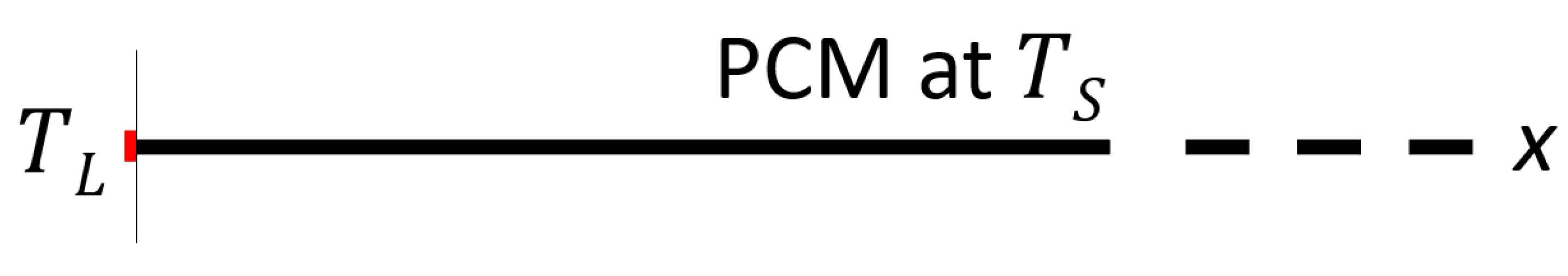
In this work, the classic two-phase Stefan problem was considered in the one-dimensional case (Figure 2): a semi-infinite slab (), initially solid at temperature , is melted from the left () by imposing a hot temperature . The problem statement is to find a temperature distribution and an interface function that satisfy [34]:
- The heat equation in both the liquid and the solid phases:where is the specific heat and is the thermal conductivity;
- The interface condition:
- The Stefan condition for the one-dimensional case:where represents the values of as ;
- The initial conditions:
- The boundary conditions:
The solution is the Neumann similarity solution which leads to the following transcendental equation for [34]:
where:
- is the Stefan number:
- ;
- is the error function;
- is the complementary error function.
The transcendental Equation (11) is a strictly increasing function of ; therefore, it intersects any horizontal line exactly once, which means that the transcendental equation has a unique root (the similarity solution is unique); therefore, if a solution exists, it is the correct solution.
Once is known, it is possible to calculate the solution using the following relationships:
- Interface location:
- Temperature in the liquid region:
- Temperature in the solid region:
2.2. Matlab Implementation of the Analytical Model
The analytical model of the classic two-phase Stefan problem (one-dimensional case) was implemented in Matlab. The main goal was to provide a tool to validate the numerical results obtained later from Ansys Fluent for the same physical problem.
The transcendental Equation (11) is solvable by the Newton–Raphson iterative method, using the value as initial approximation [34]. The Matlab script contains the Newton–Raphson function and the solution script for the two-phase 1-D Stefan problem based on Equations (12)–(14).
The Matlab script was run for a semi-infinite slab of sodium nitrate (its thermo-physical properties are reported in Table 1), initially solid at temperature , then melted from the left () by imposing a hot temperature . This phase change material, of interest to the DLR (Deutsches Zentrum für Luft- und Raumfahrt e.V.—German Aerospace Center) Thermal Process Technology Department in Stuttgart, Germany, was utilized for the numerical simulation on Ansys Fluent, as described in the next Section. It is an inorganic salt with a high phase transition temperature, chosen due to the specific application, power-to-heat-to-power. A higher phase transition temperature means higher temperature energy storage, which allows more efficient power conversion from heat to electricity. There are not many organic salts with so high a phase transition temperature and, in any case, they would have stability problems compared to an inorganic salt with the same phase transition temperature.
The comparison of results obtained from the Matlab analytical model and Ansys Fluent numerical simulation for the same boundary and initial conditions is reported in Section 4.
3. Numerical Simulation for the 1-D Problem
The numerical simulation was performed by ANSYS FLUENT 2021 R1. ANSYS FLUENT is especially suitable for analyzing solidification and melting problems because it uses a dedicated model named solidification and melting.
3.1. Solidification and Melting Model in Ansys Fluent
The solidification and melting model in ANSYS FLUENT uses an enthalpy-porosity technique to solve solidification and/or melting problems instead of tracking the moving frontier explicitly [35]. This method shows the phase change interface as a mushy porous zone where porosity is equal to the liquid fraction. The liquid fraction is associated with each cell in the computed domain and represents the fraction of the cell volume in liquid form. It changes from 0 to 1 during a melting process and from 1 to 0 during a solidification process.
The enthalpy-porosity formulation computes the liquid fraction iteration by iteration based on an enthalpy balance. When in a cell the material solidifies, and the porosity becomes 0.
The energy equation for solidification and/or melting problems is written as [35]:
where H is the enthalpy, the density, the velocity of the fluid and S the source term.
The enthalpy is calculated as:
where
is the sensible enthalpy ( is the reference enthalpy, the reference temperature and the specific heat at constant pressure), instead
represents the enthalpy of phase change ( the liquid fraction and L the enthalpy of the phase change of the material).
The liquid fraction is defined as:
- if ;
- if ;
- if .
The relation between the enthalpy and the energy is given by [36]:
3.2. Numerical Simulation of the Two-Phase 1-D Stefan Problem
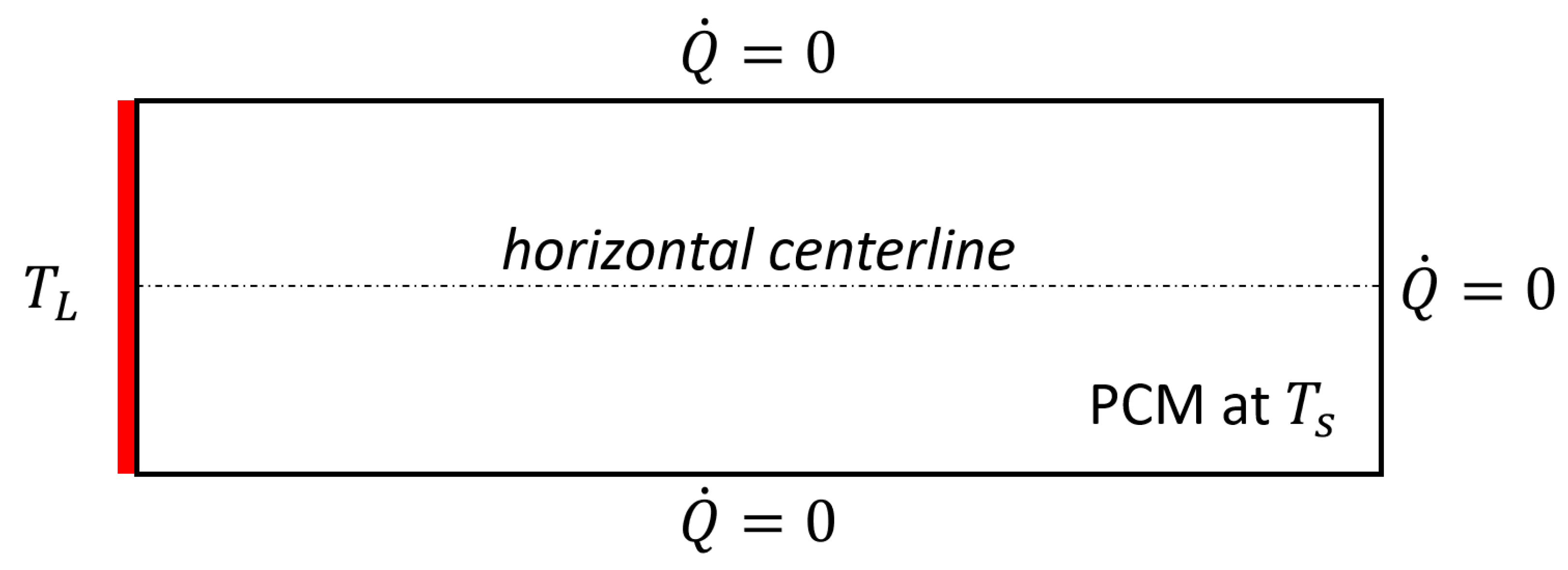
The modelling started creating the geometry with the Design Modeler tool provided by ANSYS. As shown in the schematic diagram in Figure 3, the PCM domain was a rectangle ( 10 × 3 ). The domain length was taken to be seven times as long as the area melted during the simulation to preserve the semi-infinite nature of the model. The domain height was chosen to make the system’s behaviour nearly 1D along the horizontal centerline, where results were used for the comparison with two-phase 1-D Stefan problem analytical model.
The mesh was generated using uniform quadrilaterals with an element size of .
The problem was solved by the finite volume method using ANSYS FLUENT 2021 R1. The procedure followed for the model setup is described in the following:
- In General, the solver was set to time-transient and 2D-planar analyses. The gravity contribution was not considered;
- In Models the solidification and melting model was set to on, automatically enabling the energy model; the viscous flow model was changed from SST k-omega to laminar;
- In Materials, the phase change material (NaNO3) was created, uploading the properties reported in Table 1;
- In Boundary Conditions, the left wall temperature was set to ( 350 ), while the top, right and bottom sides were perfectly insulated (heat flux equal to zero);
- In Solution Methods, pressure and velocity coupling was realized by the SIMPLE algorithm. Momentum and energy equations were discretized using a second-order upwind interpolation scheme, while the pressure equation was solved with the second-order method. The gradient discretization adopted the least-squares-cell-based method. The transient formulation that discretized the governing equations used the implicit first-order Euler method;
- In Solution Controls, all the under-relaxation factors were left to the default values;
- In Solution Initialization, the initial value of was set to ( 300 ).
Calculations were performed using an adaptive CFL-based method for time advancement with incremental time steps. The time step was set to for 18,000 time steps (total flow time: ). The maximum number of iterations per time step was set to 30. Convergence was obtained when the residual of equations was less than 1 × 10.
4. Validation of the Numerical Model
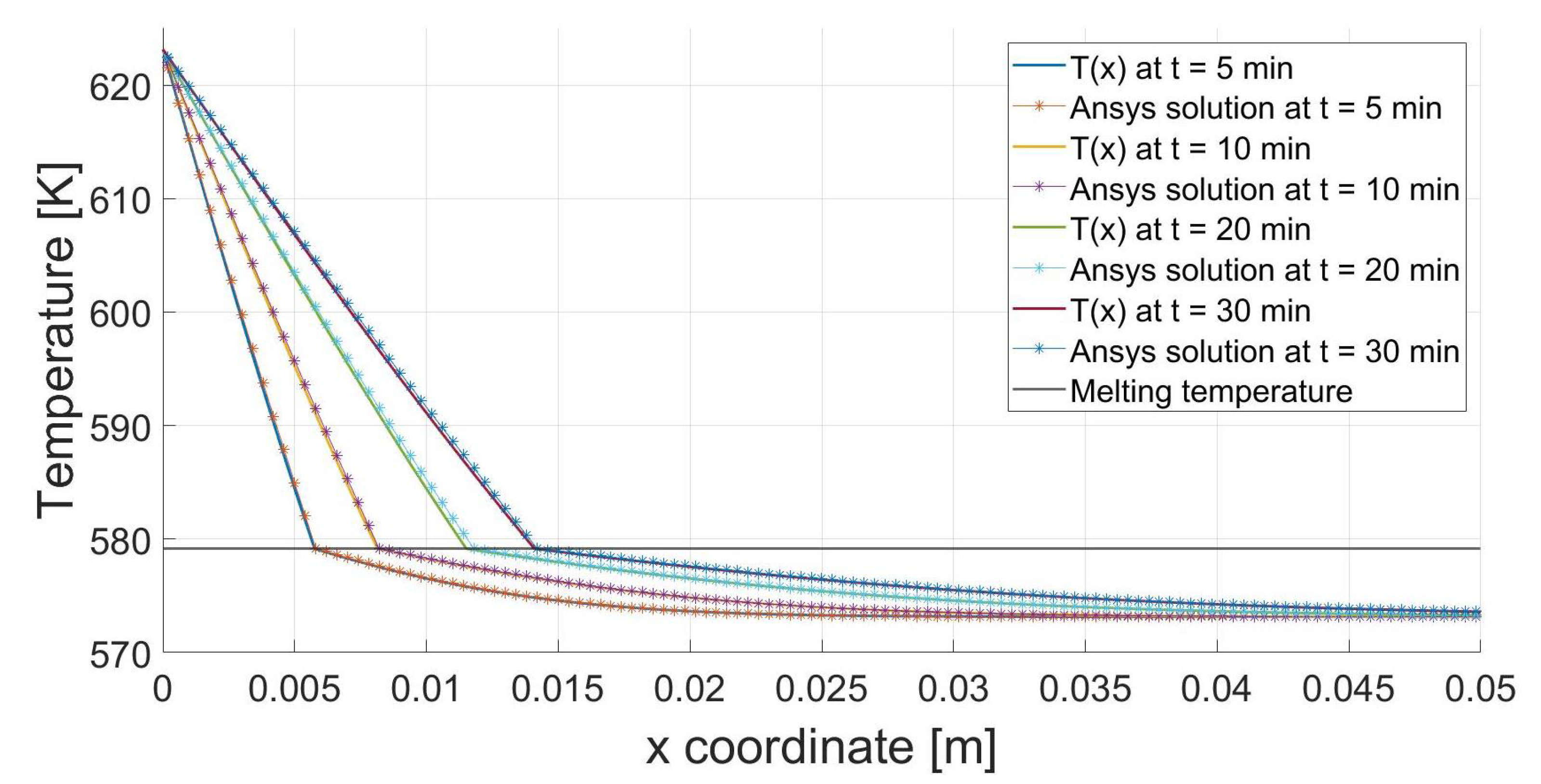
Figure 6 plots the temperature profile along the x coordinate, calculated from both the analytical and numerical models at 5 min, 10 min, 20 min and 30 min.
is the i-th point of the discretized domain along the horizontal centerline, and are the temperature results calculated in the i-th point of the discretized domain at a time , respectively, from the analytical and numerical models.
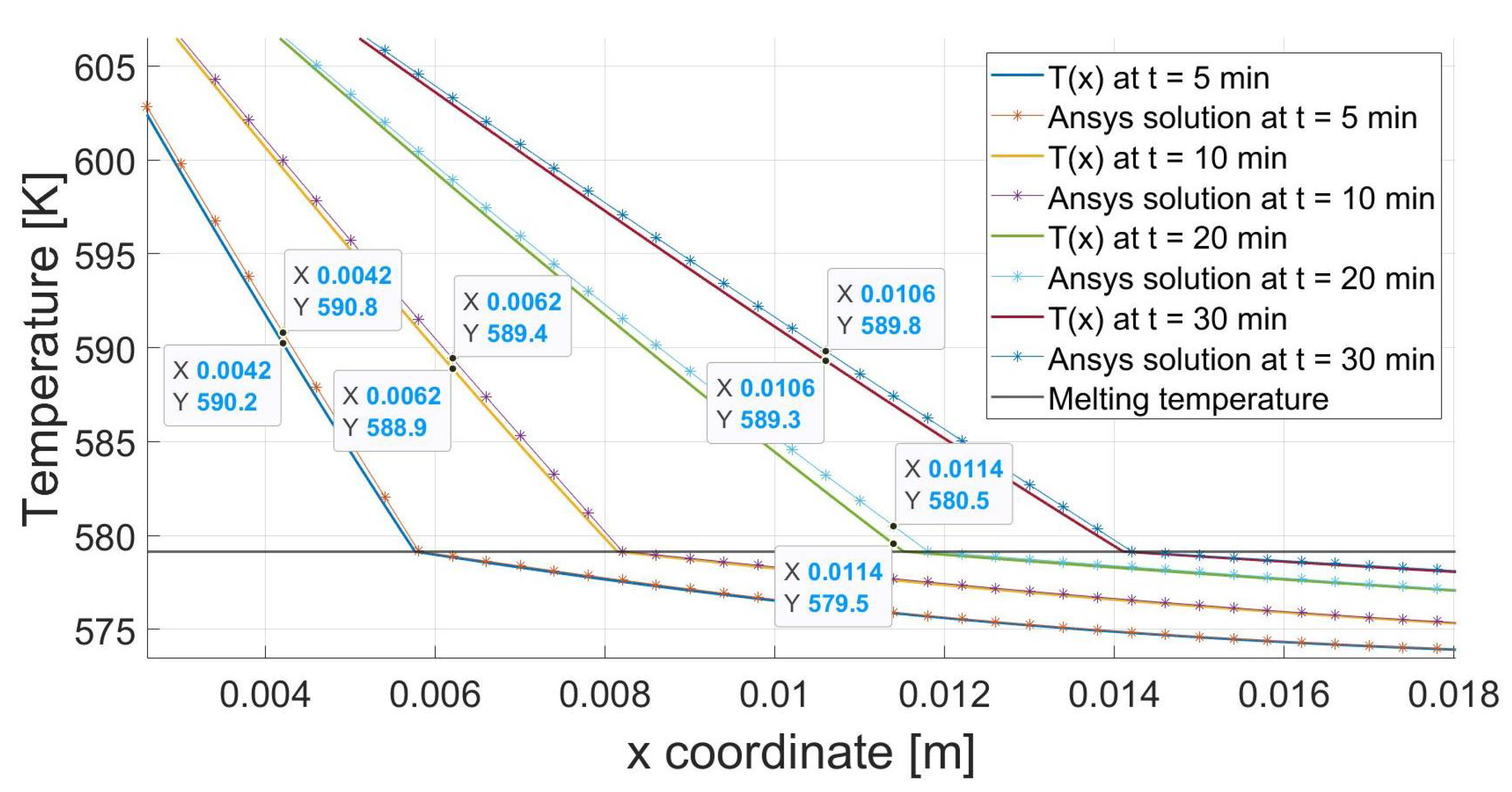
Table 2 shows the maximum computational error on the temperature field at 5 min, 10 min, 20 min and 30 min. The x coordinates and the temperature values corresponding to the calculated maximum errors are reported in Figure 7. All the errors are less than 2%, indicating the goodness of the correspondence between numerical and analytical results.
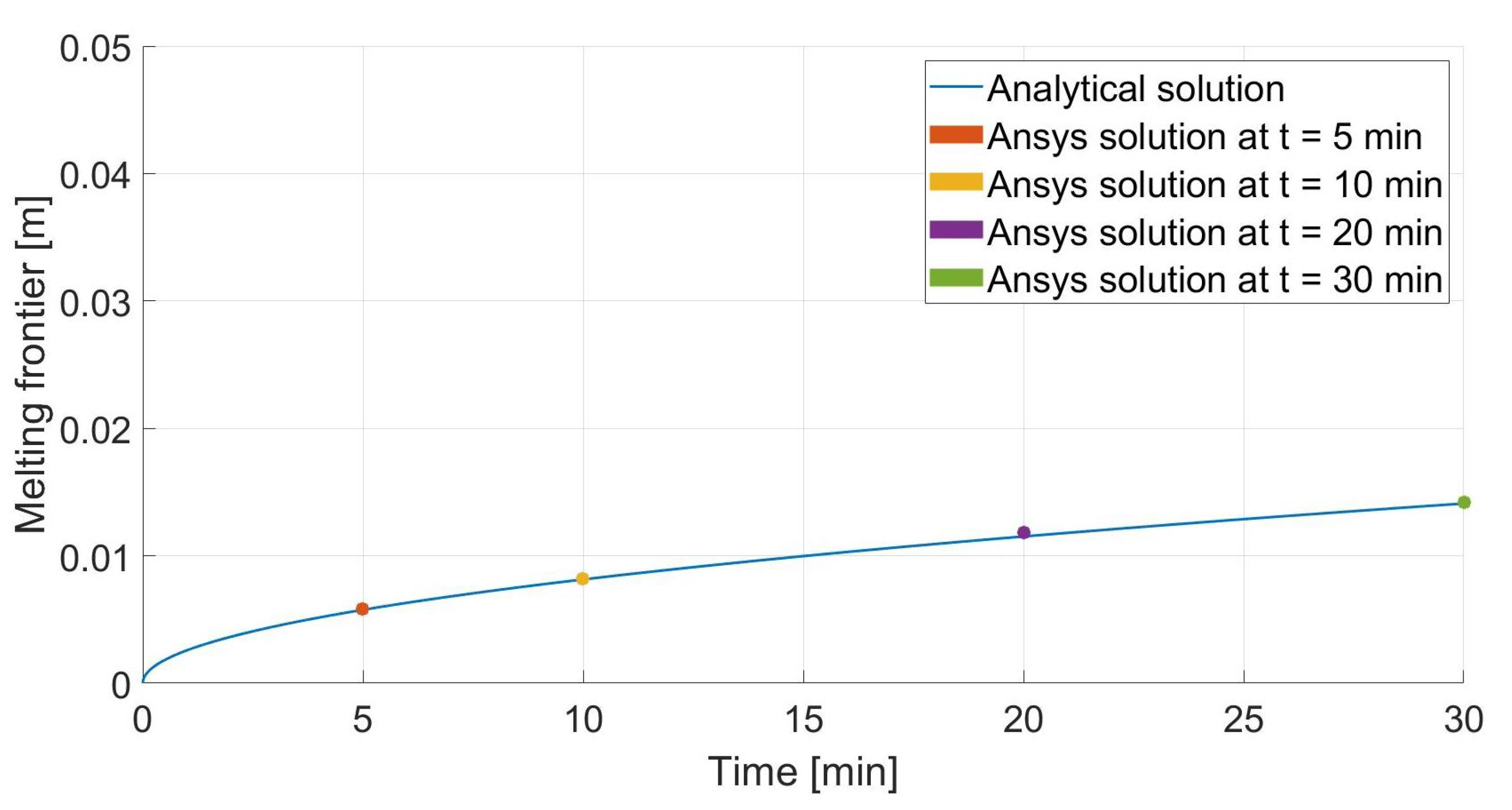
Figure 8 plots the frontier position over time, calculated from both the analytical and numerical models (at 5 min, 10 min, 20 min and 30 min).
is the i-th time of the simulation, and are the interface position calculated at time , respectively, from the analytical and numerical models.
Table 2 shows the computational errors on the interface position at 5 min, 10 min, 20 min and 30 min. In addition, in this case, all the errors are small (the maximum computational error is 2.5%).
The validation of the results obtained from the numerical simulations confirm the correctness of the numerical model settings described in Section 3.2. The same settings can be used for studying a more complicated geometry in a more interesting problem.
5. Numerical Simulations for the Finned Tube
Sure about the numerical model settings described in Section 3.2, the research work aims now to study a more interesting problem, evaluating the performance of different latent heat TES configurations during the discharging process: the system, initially charged (this means all the PCM is liquid), undergoes a sudden decrease in temperature, starting to discharge (solidification process) and release heat to the heat transfer fluid. The work aims to find the most efficient latent heat TES configuration in terms of a maximum average discharging power.
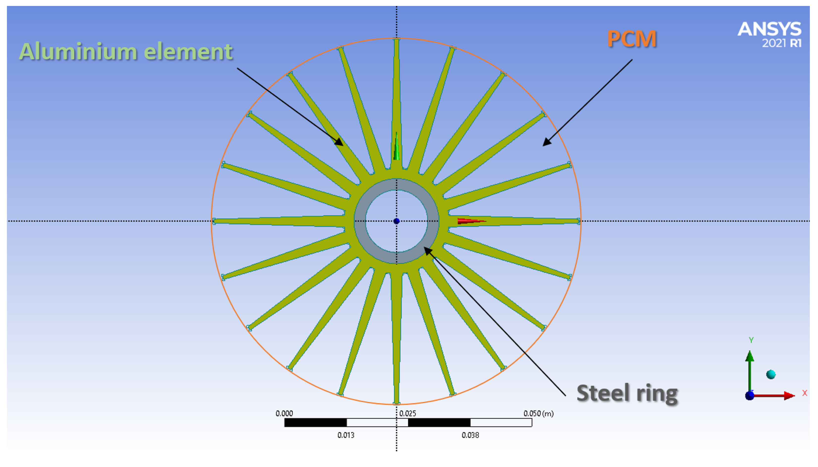
The analysis deals with three different axial structures connected to the heat transfer tube (one of the three two-dimensional geometries is shown in Figure 9). All the geometries consist of:
- A steel inner tube in which the heat transfer fluid flows (it does not change in the comparison);
- An aluminium heat conduction structure connected to the heat transfer tube;
- The PCM all around the aluminium structure up to its outer radius.
Geometries were sized with the following criteria:
- They change only for the fin shape (rectangular, trapezoidal and fractal fins);
- The three different structures connected to the heat transfer tube have the same volume fraction;
- The PCM mass is constant in all the configurations, which means that the PCM volume fraction is also constant.
The volume fraction is calculated as:
where x stands for steel, aluminium and PCM; is the surface area covered by x-material; is the surface area of the cycle that has the distance from the fin tip to the tube centre as radius and L is the length of the TES system (it will be considered equal to 1 m for the calculation of the total discharging power).
As stated before, the volume fractions are kept constant for all the configurations (constant radial dimensions) to perform a proper comparison that evaluates only the shape of the fins. Table 3 reports the constant parameters for the three configurations.
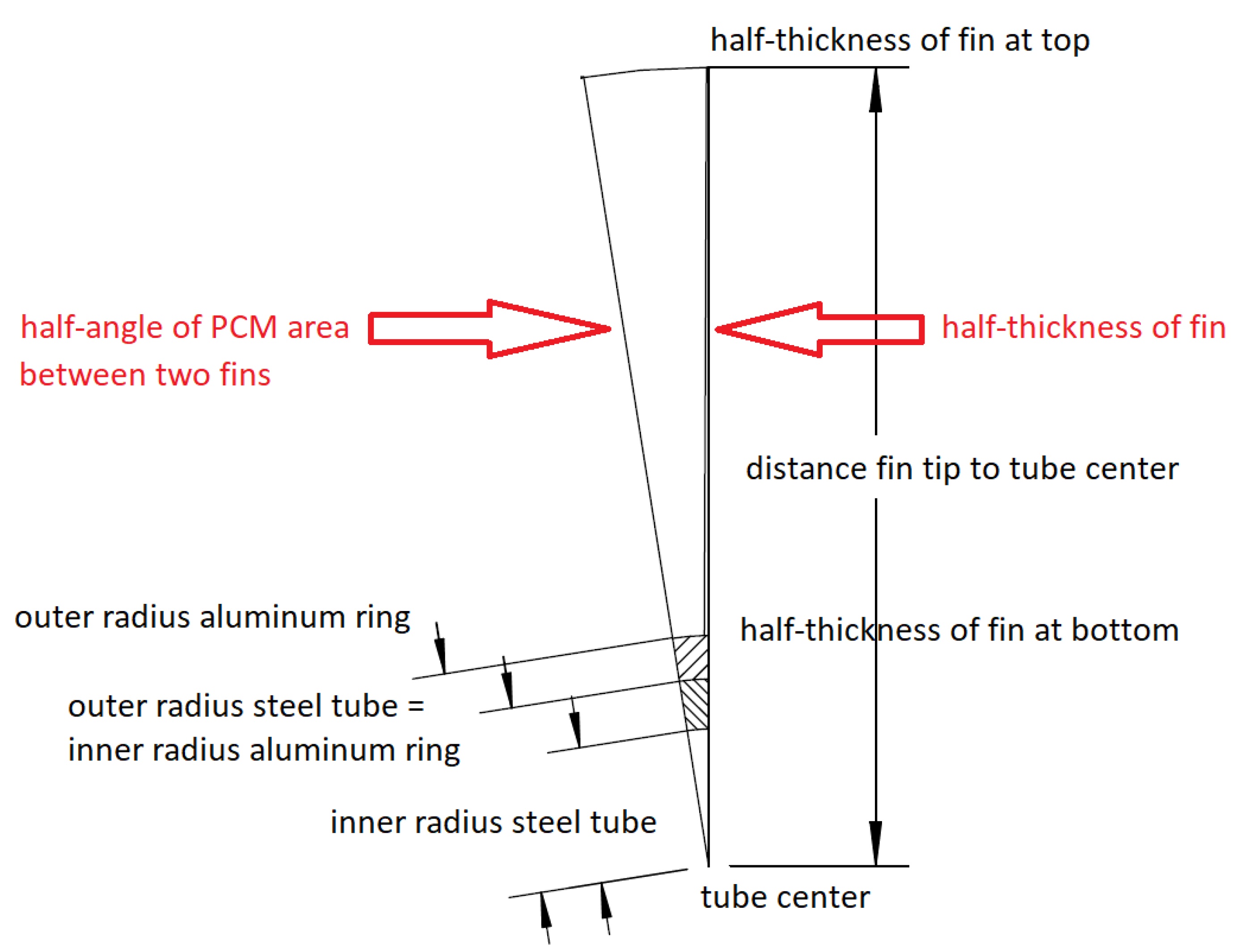
Again, numerical simulations were performed using ANSYS FLUENT 2021 R1. Geometry domains, created with the Design Modeler tool, represent only a section of the total domain, thanks to the symmetry of the model. In particular, the drawn section considers the fin’s half-thickness and the PCM area’s half-angle between two fins, as shown in Figure 10 for one of the three configurations. The angle of the simulated section is 9° as all the models have 20 fins.
Once a drawing in Design Modeler was completed, the three domains (steel aluminium and PCM) were selected to make all into one part; in this way, Ansys Fluent does not solve equations in the contact regions but just considers the thermophysical property changes between domains.
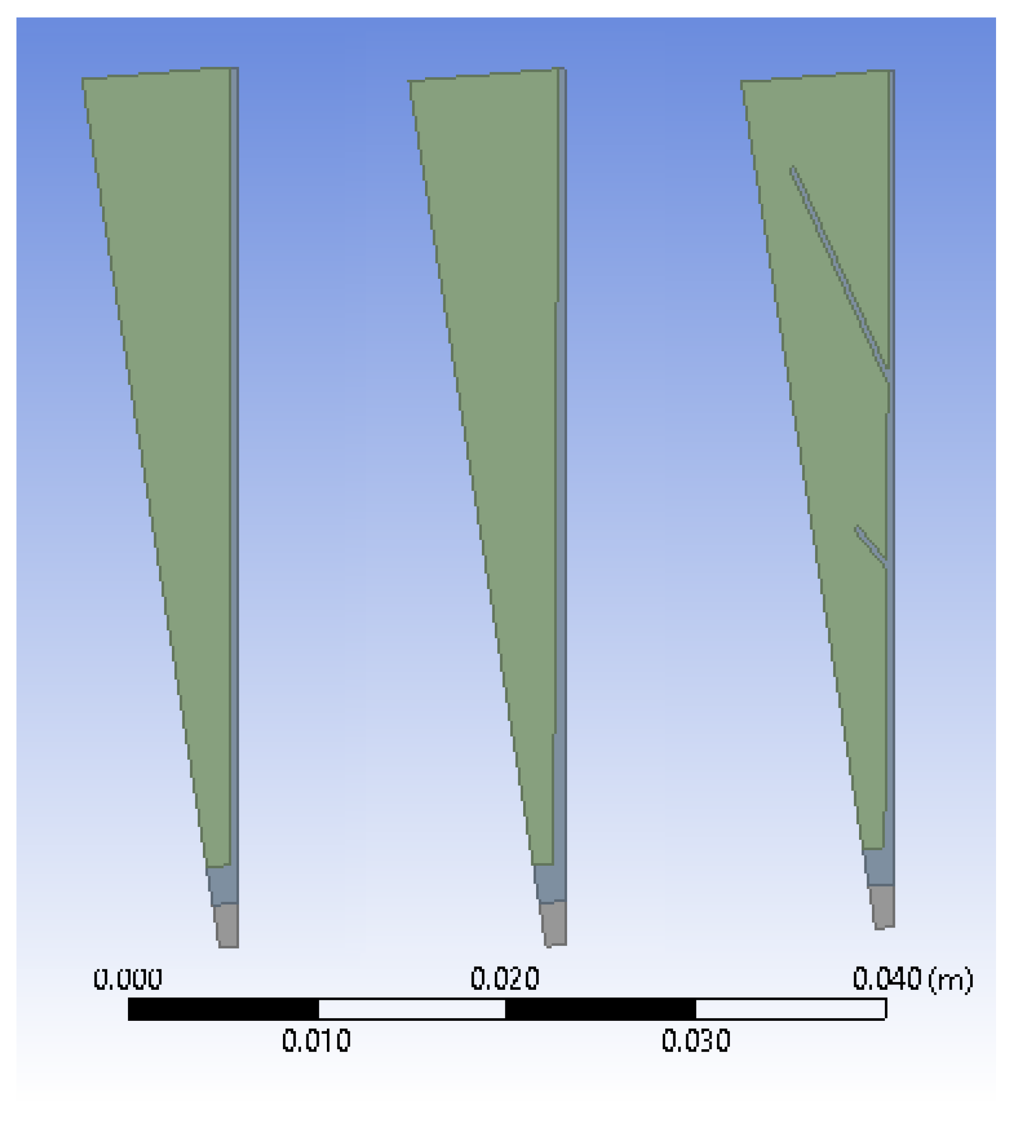
According to all the previous considerations, the simulated domains for the three axial structures are reported in Figure 11.
The meshes were generated using non-regular quadrilaterals elements with an element size of , and have a number of nodes and elements reported in Table 4 for each configuration.
The problem was solved using the finite volume method of ANSYS FLUENT, using the same settings of the 1D model reported in Section 3. In addition, in these simulations, convection is neglected. In the 1D model, the reason for ignoring convection was to perform the comparison with the analytical model of the classical two-phase Stefan problem, in which equations cannot take into account convection (see the simplifying assumptions described in Section 2.1). Here, the system is perfectly insulated (no thermal flow, no heat dispersion, no border effects), except for the wall in which the discharging temperature is applied; furthermore, as the initial condition, the PCM domain is totally liquid but at the same temperature (no thermal gradient). According to these assumptions, it is reasonably possible to neglect convection, considering that this choice yields a conservative estimate of the melting speed.
NaNO3 is the phase change material used for finned tube simulations (its properties are reported in Table 1). It was initially liquid at temperature , more than the melting temperature () in order to have a 100% liquid fraction at time on ANSYS FLUENT simulator.
As boundary conditions, a temperature difference of was imposed at the inner radius of the steel ring while all the other boundaries are perfectly insulated (heat flux equal to zero).
The calculations were performed using an adaptive CFL-based method for time advancement with incremental time steps. The time step was set to for 48,000 time steps (total flow time: ).
Results and Discussion
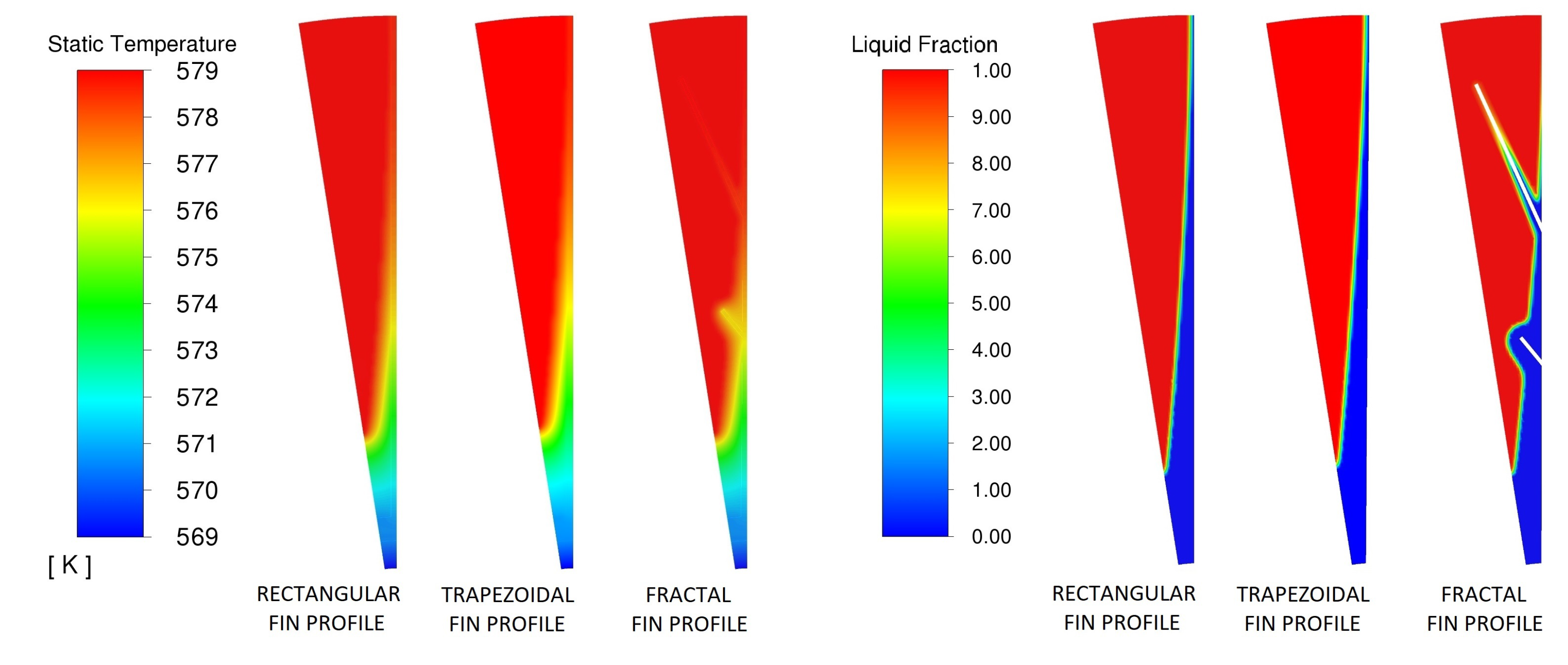
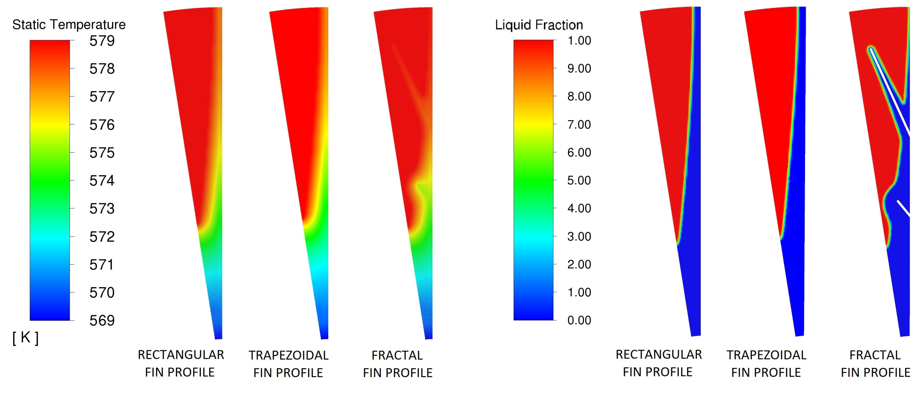
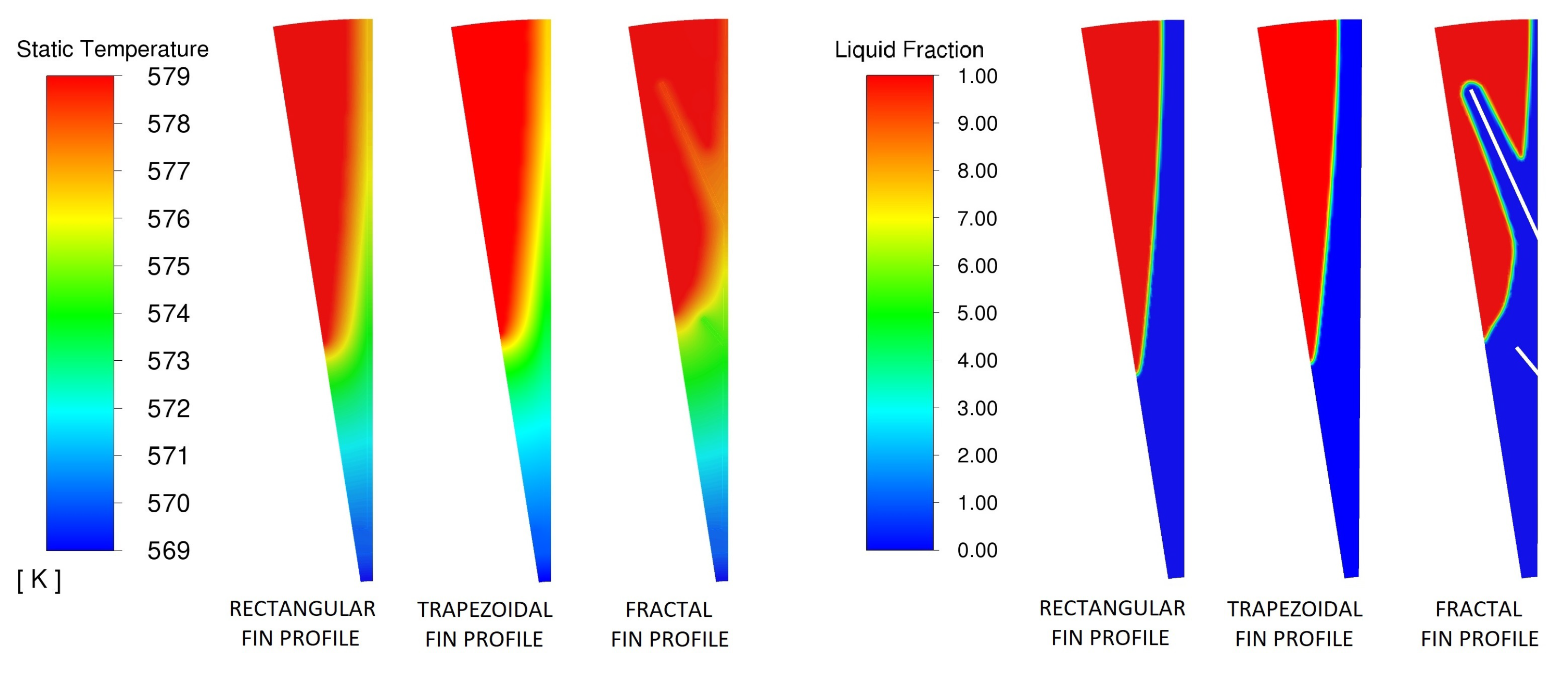
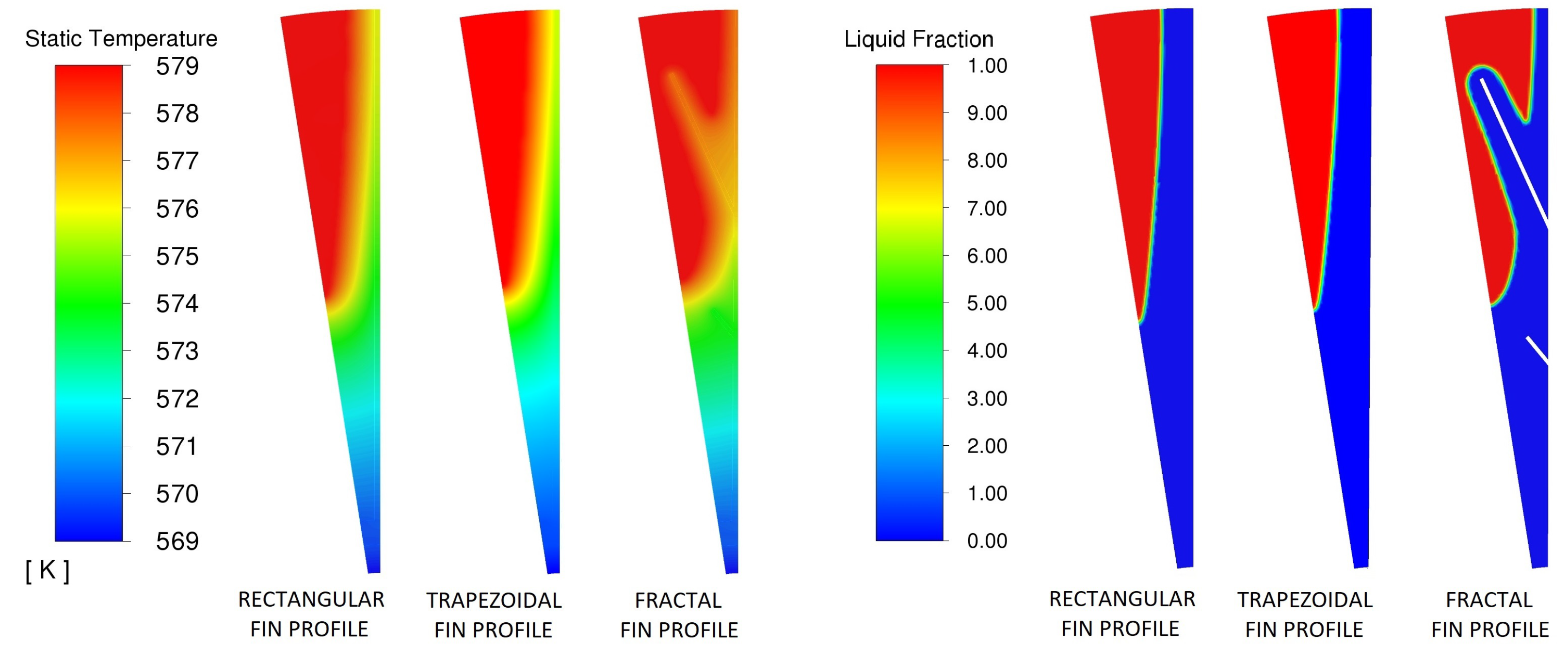
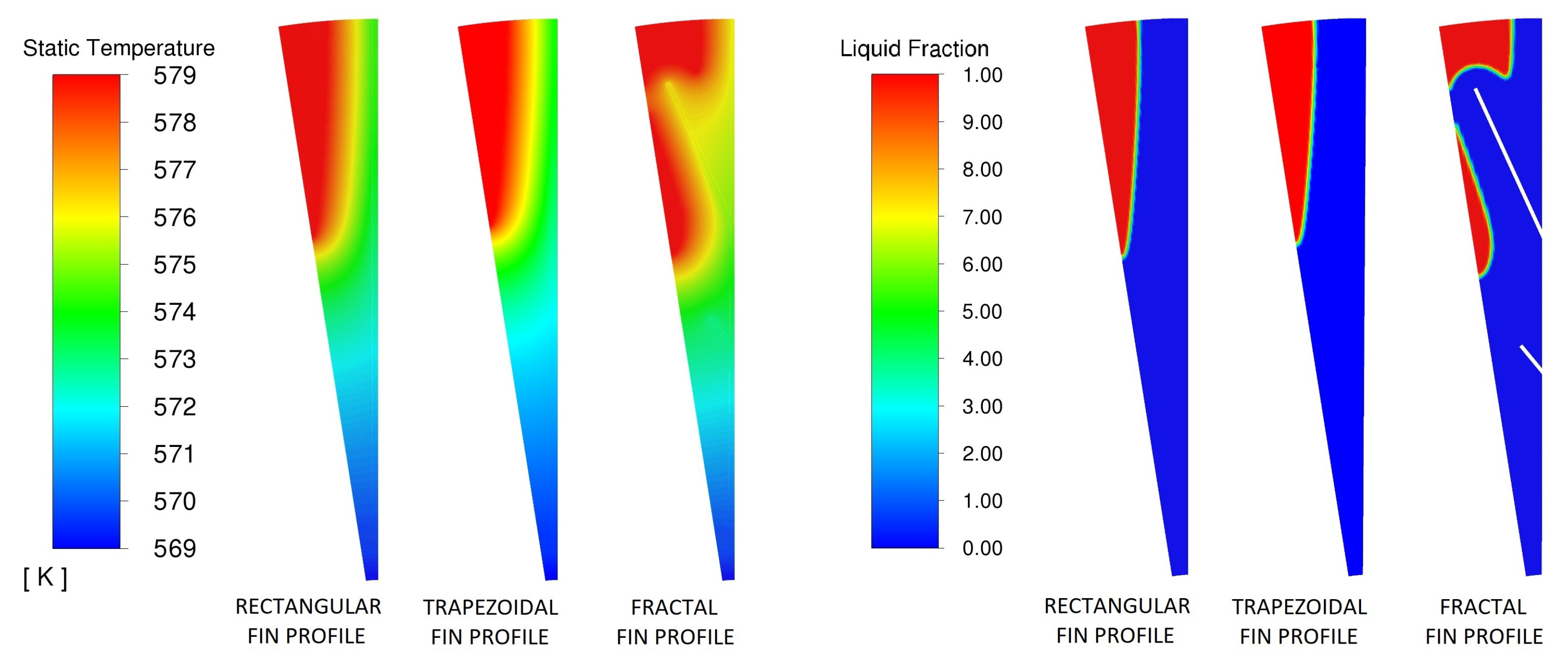
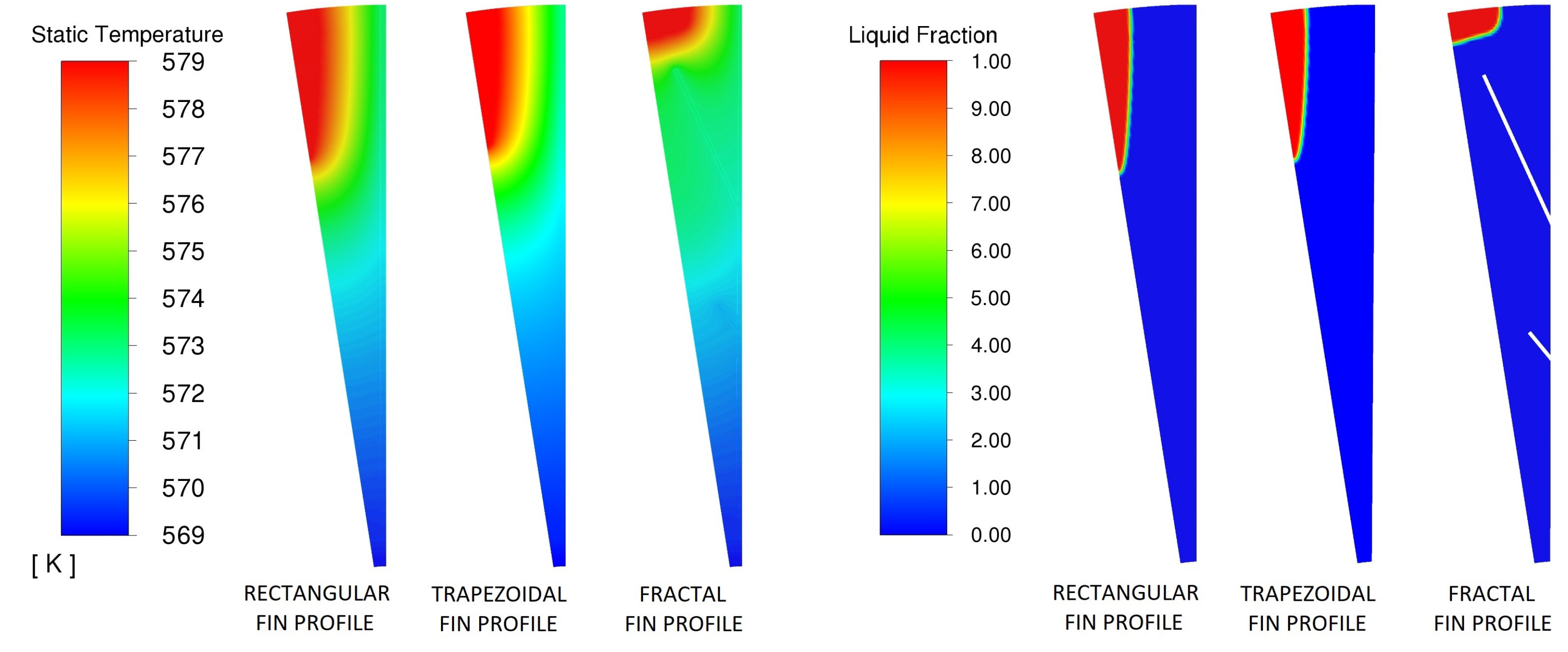
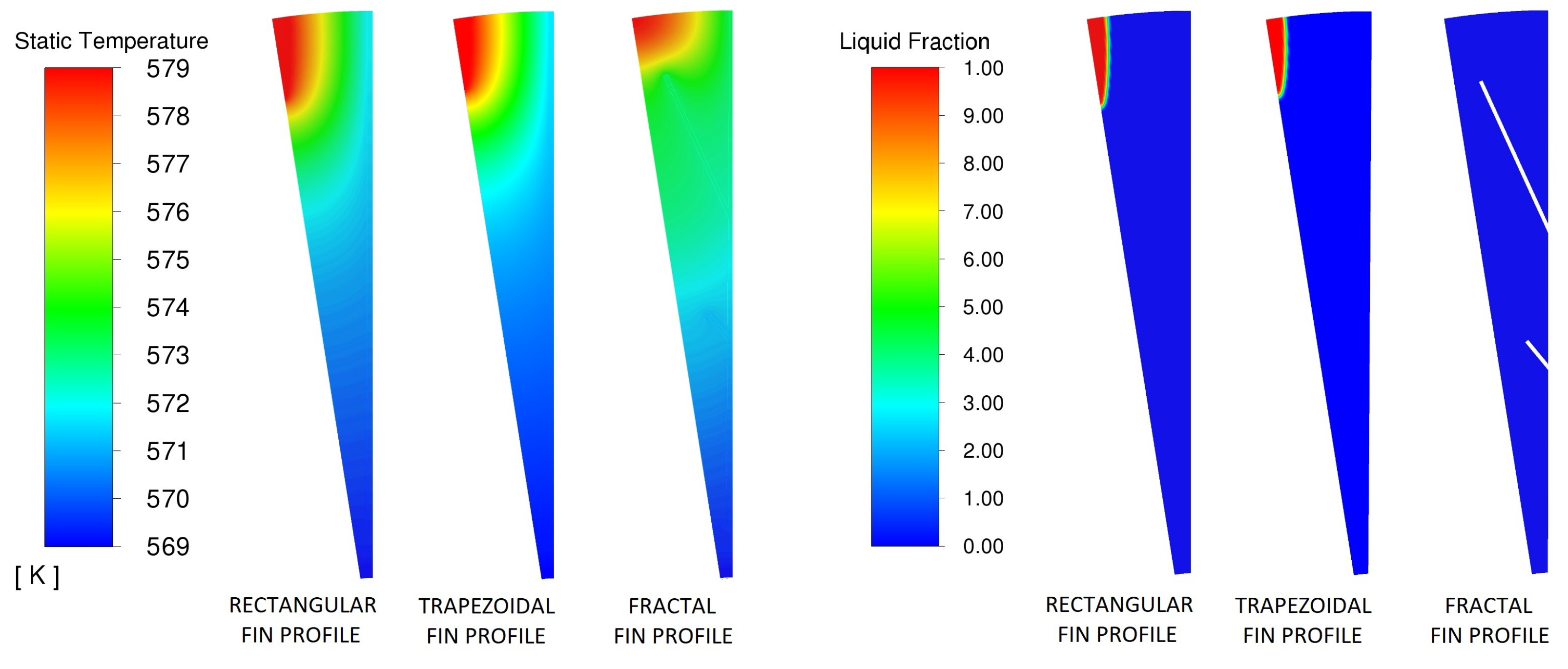
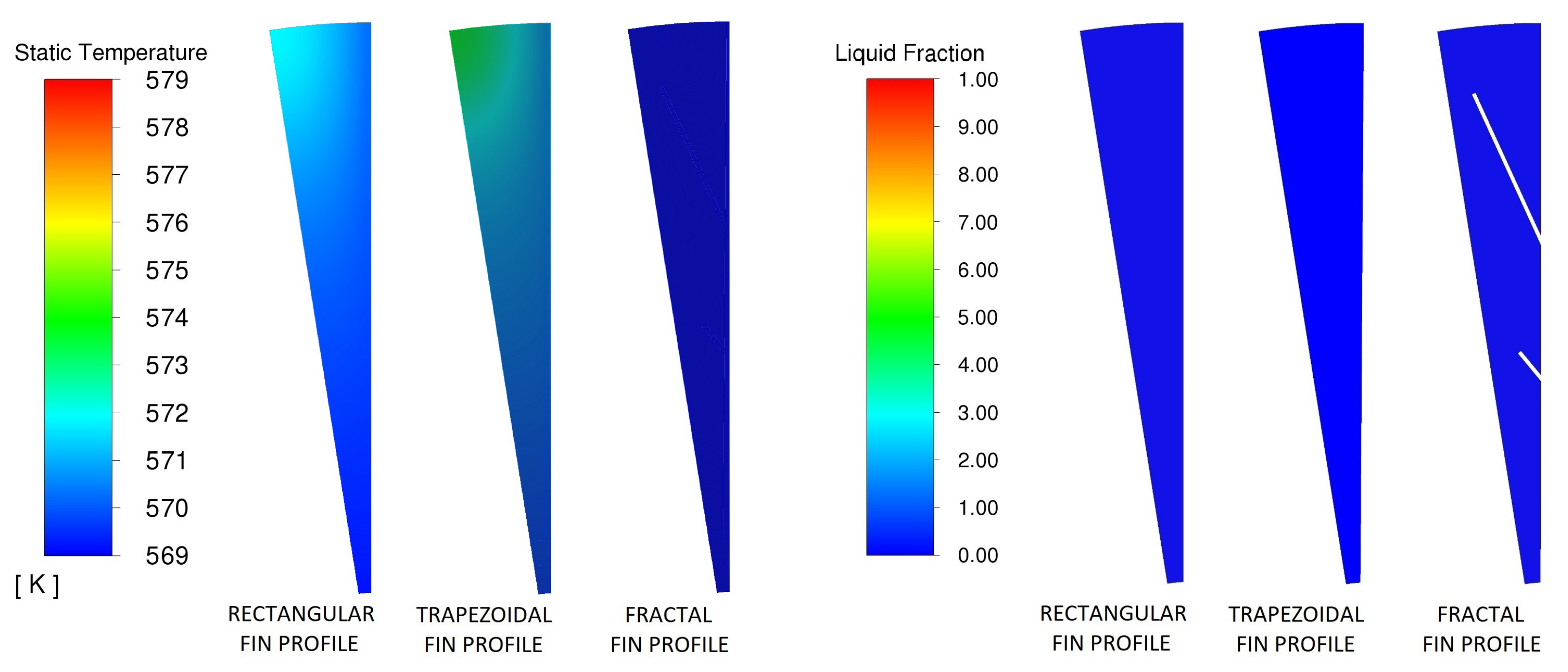
Figure 12, Figure 13, Figure 14, Figure 15, Figure 16, Figure 17, Figure 18 and Figure 19 show temperature and liquid fraction contours for all the configurations at 5 min, 10 min, 15 min, 20 min, 30 min, 40 min, 50 min and 60 min.
In the rectangular fin profile geometry all the PCM was discharged at t = 60 min (liquid fraction equal to 0%, Figure 19, Table 5).
In the trapezoidal fin profile geometry, too, all the PCM was discharged at t = 60 min; furthermore, the liquid fraction was always slightly lower than in the previous case (Table 5). This means that the trapezoidal fin profile performs more than the rectangular one.
In the fractal fin profile geometry, the profile seems to be worse than the previous configurations, but only at the beginning of the discharging process (t < 15 min, Table 5); indeed, from t = 15 min, the performance of the fractal fin profile is the best. This behaviour is due to the different distribution of the aluminium material between configurations: the non-fractal profiles have more aluminium content near the connection with the heat transfer tube where the phase change starts, so the thermal exchange is faster at the beginning of the solidification process. On the contrary, the fractal profile has lower aluminium content at the bottom of the fins because of the branches (the aluminium fraction is constant for all the configurations), but the branches are responsible for faster thermal exchange when the solidifying frontier moves away from the steel ring.
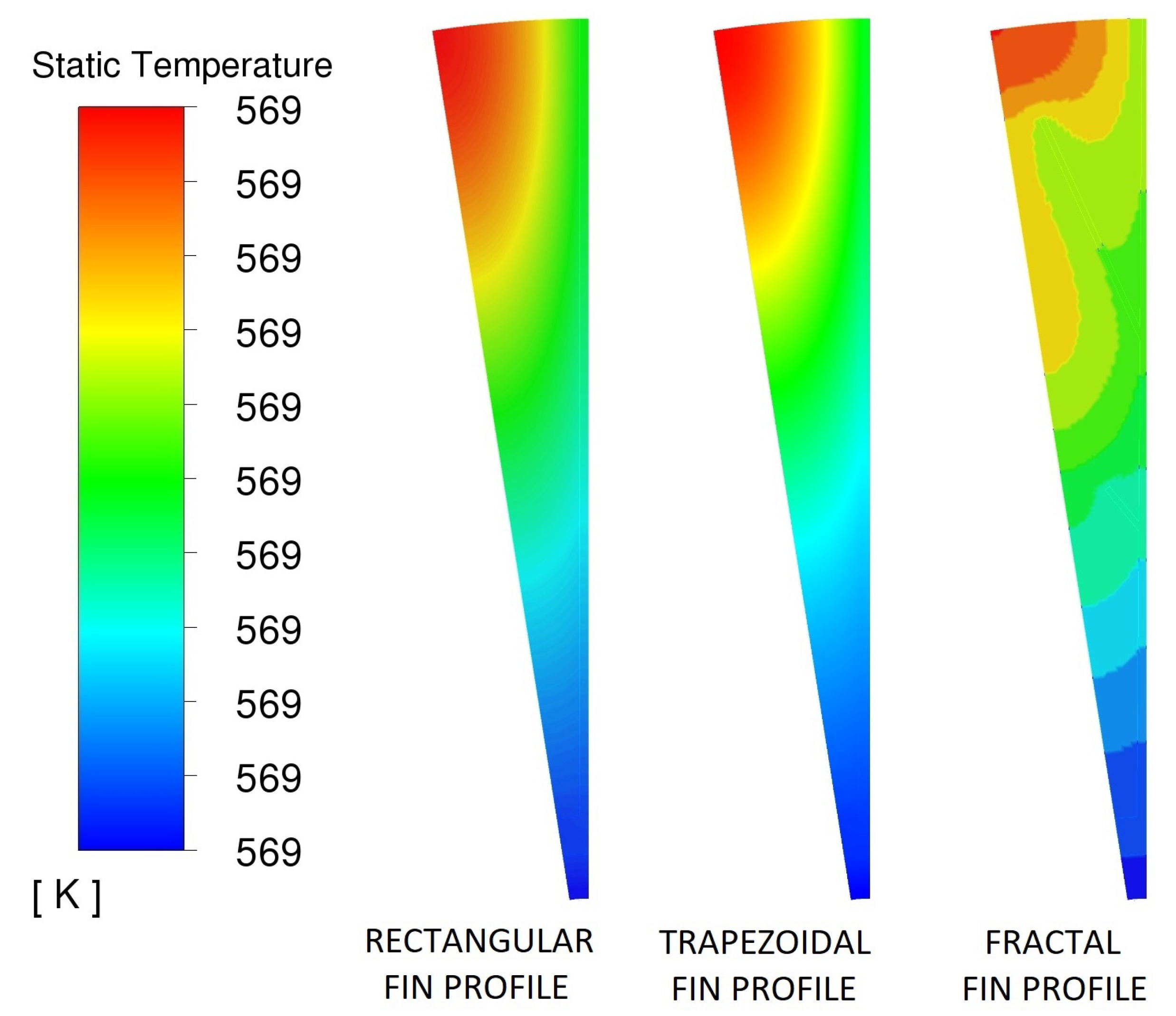
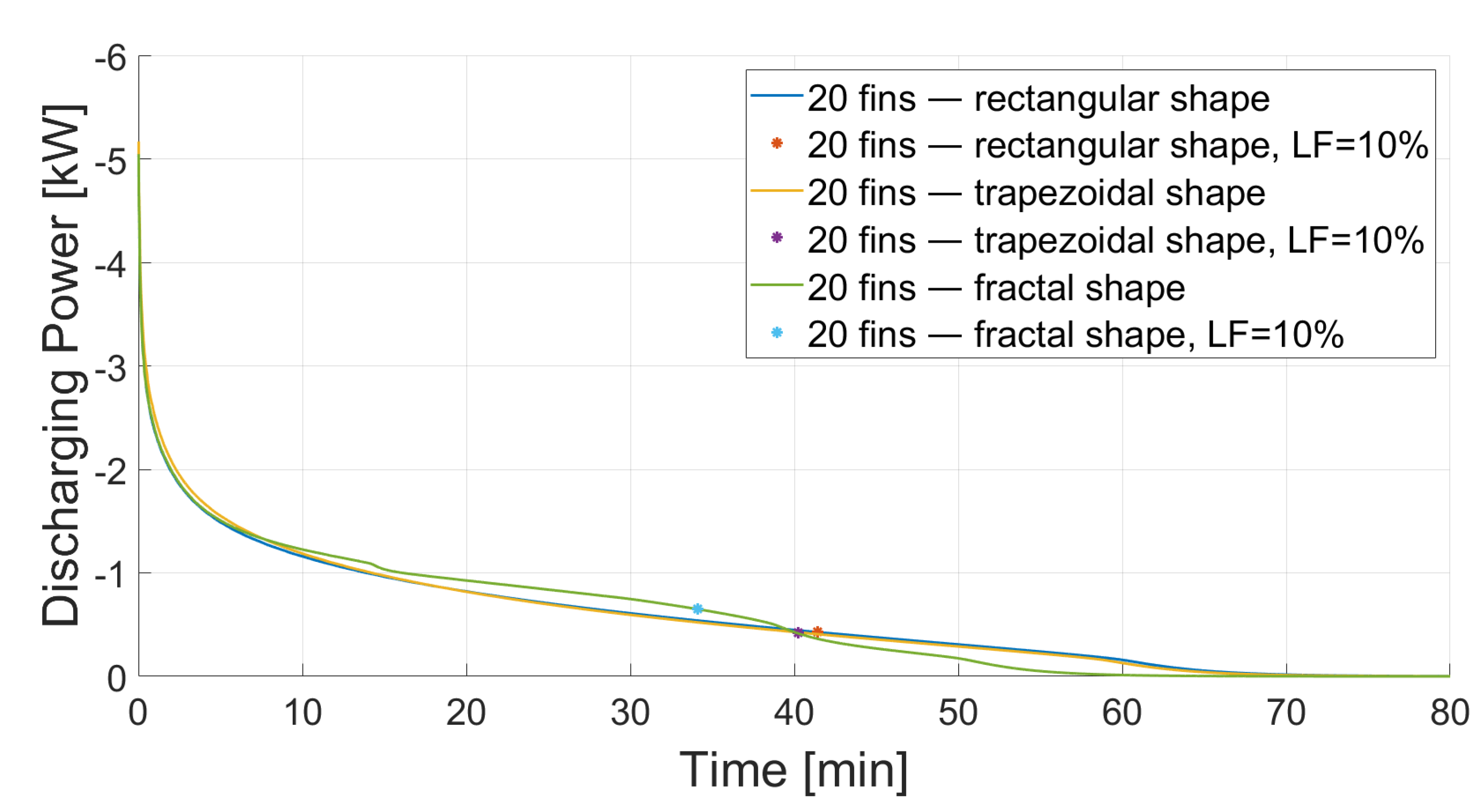
Temperature contours for the three configurations at the end of the simulation time (t = 80 min) are reported in Figure 20. They show that all the energy is released because the temperature field equals the imposed temperature throughout the domain. It can also be seen through the discharging power graph over time, reported in Figure 21, that the power is equal to zero at t = 80 min.
A discharging power graph (Figure 21) was calculated from the total heat flux ( / ) at the inner radius of the steel tube for a 1 length TES system. To perform the comparison between curves, the point where the liquid fraction equals a reference value (10%) is also represented in the graph, showing a faster discharging speed for the fractal geometry.
The fractal fin profile shows an inflection point at 40 min. This is due to the complete solidification of the PCM between the branches which caused the modification of the thermal conduction pattern. This has a direct impact on the discharging power.
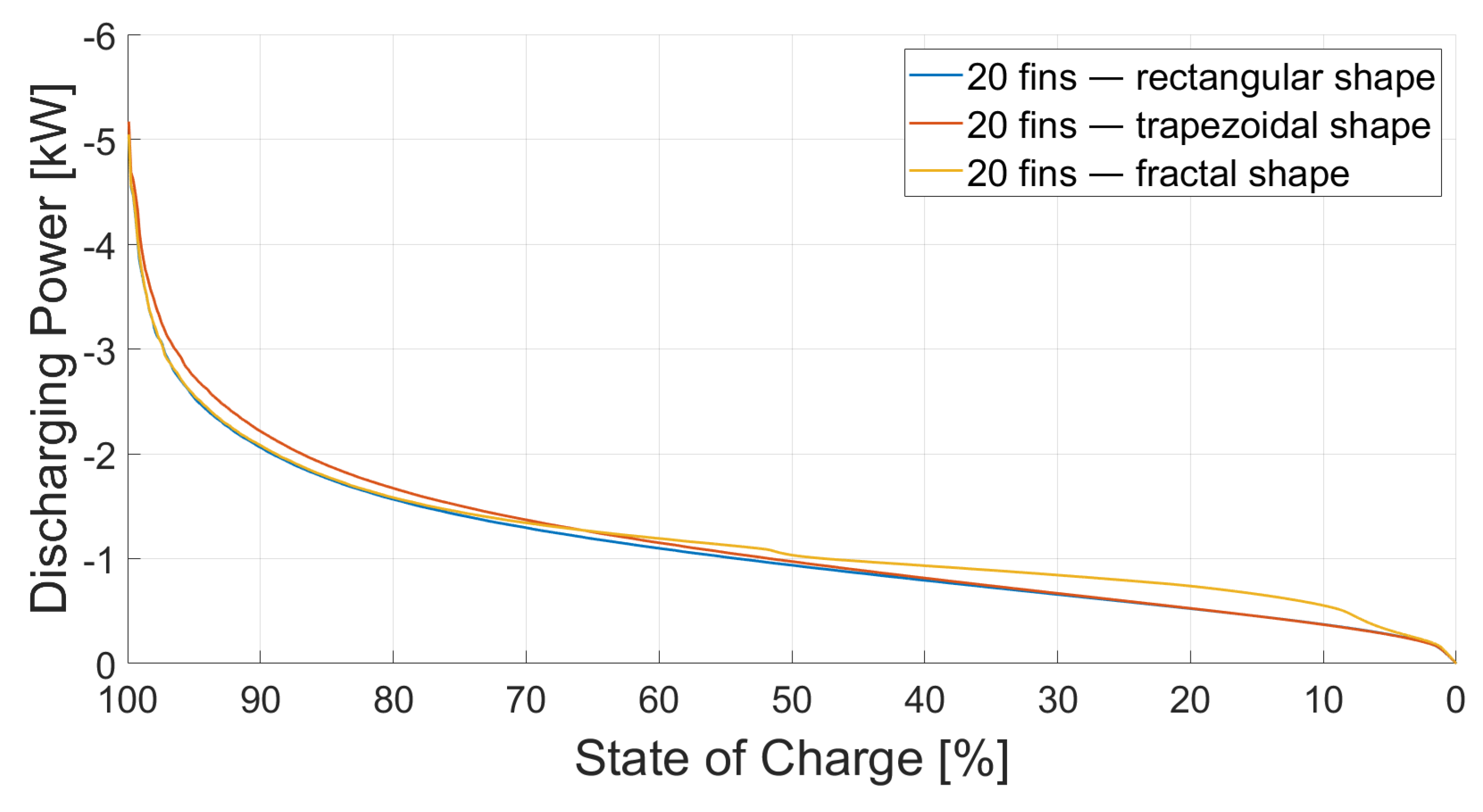
Figure 22 shows the discharging power curve over the state of charge of the thermal battery which varies from 100% (system completely charged, all PCM liquid) to 0% (system completely discharged, all PCM solid). If is the initial time and is the time corresponding to the end of the simulation, the state of charge is calculated as:
where represents the PCM accumulated energy at time t and the total PCM released energy until complete solidification. The energy, calculated by Ansys Fluent according to the Equation (19), is here the average energy calculated over the PCM area at time t, and .
The reference value of 10% liquid fraction, mentioned above, is also used to calculate the average discharging power as:
where:
- is the time corresponding to LF = 10%;
- is the initial time;
- is the time discretization index;
- is the discharging power corresponding to the i-th time step;
- is the time corresponding to the i-th time step.
The average discharging power for the three configurations is reported in Table 6, together with the total energy released during the discharging process up to the end of the simulation. The total energy was calculated:
- Theoretically aswhere [ ] is the PCM total mass of a 1 length TES system and L ( / ) is the PCM enthalpy of phase change;
- From the discharging power curve (at the inner radius of the steel tube) aswhere is the time corresponding to the end of the simulation, is the time discretization index, is the discharging power corresponding to the i-th time step and is the time corresponding to the time step.
represents the storage capacity of the thermal battery as it is calculated from the PCM mass and enthalpy of phase change of the TES system (for this reason, it is a positive value). It is constant for all the configurations (Table 6) as they are created to keep constant the PCM volume fraction.
is a negative value as it represents the total energy released during the discharging process. It slightly changes for the three configurations due to the different domain discretization and its absolute value is higher than because of the energy contributions of aluminium and steel materials.
6. Conclusions and Future Developments
In this study, long-term thermal-energy storage was investigated; in particular, a latent heat alternative among TES solutions.
The classical Stefan problem was considered in the one-dimensional case in order to implement its analytical model in Matlab. The transcendental equation was solved by the Newton–Raphson iterative method. The same boundary and initial conditions were utilized for the numerical simulation on ANSYS FLUENT 2021 R1, then the comparison of results obtained from the Matlab analytical model and Ansys Fluent numerical simulation was carried out. The maximum computational error was less than 2.6%.
The validation of the results allowed us to be confident about the correctness of the numerical model settings, so the same settings were used for studying a more interesting problem, i.e., evaluating the performance of three different latent heat TES configurations during a discharging process. The goal was to find the most efficient latent heat TES configuration in terms of maximum average discharging power. Geometries were sized changing only the fin shape (rectangular, trapezoidal and fractal), keeping constant the volume fractions of steel, aluminium and PCM for all the configurations to perform a proper comparison. Results showed that the trapezoidal fin profile performs better than the rectangular one. The fractal fin profile geometry seemed worse than the others at the beginning of the discharging process due to the different distributions of the aluminium material between configurations. Instead, it was definitively revealed to be the best at the end, as the branches are responsible for faster thermal exchange when the solidifying frontier moves away from the steel ring. The PCM was completely discharged after 50 min (PCM in rectangular fin profile geometry after 59 min and in the trapezoidal fin profile geometry after 58 min). This behaviour was also shown from the discharging power graph over time and over the state of charge. In conclusion, the average discharging power for the three configurations was evaluated, showing the higher performance obtained with the fractal fin profile.
The implemented model can be utilized as a tool for the design of thermal-energy storage systems based on PCM (such as Carnot batteries). A direct application of this tool was used to find a preliminary design of the CHESTER project TES system. The numerical model is also suitable for simulating PCM with conductive additives, requiring only changes in the thermophysical properties of the material. Future developments foresee other simulations with such phase change materials or with the same PCM used in this work but utilizing the thermophysical properties obtained from experimental measurements. The next step will be the experimental validation of the same physical models numerically studied in this work.
Author Contributions
Conceptualization, E.P., R.C., F.M. and S.V.; Investigation, E.P., R.C. and S.V.; Methodology, S.V.; Software, E.P.; Writing—original draft, E.P. All authors have read and agreed to the published version of the manuscript.
Funding
This research was developed and partially funded within the EERA JP ES (European Energy Research Alliance Joint Programme for Energy Storage) mobility scheme.
Data Availability Statement
Not applicable.
Acknowledgments
The authors are thankful for the support given by the DLR (Deutsches Zentrum für Luft- und Raumfahrt e.V.)—German Aerospace Center, in Stuttgart, Germany (in particular to Andrea Lucia Gutierrez Rojas, Wolf-Dieter Steinmann and Larissa Dietz), where this study was carried out within the CHESTER project. An acknowledgment also to the EERA JP ES (European Energy Research Alliance Joint Programme for Energy Storage), which contributed to the research collaboration between the DLR, the CNR and the University of Catania.
Conflicts of Interest
The authors declare no conflict of interest.
References
- Gielen, D.; Boshell, F.; Saygin, D.; Bazilian, M.D.; Wagner, N.; Gorini, R. The role of renewable energy in the global energy transformation. Energy Strategy Rev. 2019, 24, 38–50. [Google Scholar] [CrossRef]
- Ley, M.B.; Jepsen, L.H.; Lee, Y.S.; Cho, Y.W.; Bellosta von Colbe, J.M.; Dornheim, M.; Rokni, M.; Jensen, J.O.; Sloth, M.; Filinchuk, Y.; et al. Complex hydrides for hydrogen storage—New perspectives. Mater. Today 2014, 17, 122–128. [Google Scholar] [CrossRef] [Green Version]
- Mackay, D.J. Sustainable Energy—Without the Hot Air; Uit Cambridge Ltd.: Cambridge, UK, 2009. [Google Scholar]
- Trebilcock, F.; Ramirez Stefanou, M.; Pascual, C.; Weller, T.; Lecompte, S.; Hassan, A. Development of a Compressed Heat Energy Storage System Prototype. In Proceedings of the IIR Rankine 2020 Conference—Advances in Cooling, Heating and Power Generation, Virtual, 27–31 July 2020. [Google Scholar] [CrossRef]
- Katsaprakakis, D.A.; Dakanali, I.; Condaxakis, C.; Christakis, D.G. Comparing electricity storage technologies for small insular grids. Appl. Energy 2019, 251, 113332. [Google Scholar] [CrossRef]
- Arnaoutakis, G.E.; Kefala, G.; Dakanali, E.; Katsaprakakis, D.A. Combined Operation of Wind-Pumped Hydro Storage Plant with a Concentrating Solar Power Plant for Insular Systems: A Case Study for the Island of Rhodes. Energies 2022, 15, 6822. [Google Scholar] [CrossRef]
- Elberry, A.; Thakur, J.; Santasalo-Aarnio, A.; Larmi, M. Large-scale compressed hydrogen storage as part of renewable electricity storage systems. Int. J. Hydrogen Energy 2021, 46, 15671–15690. [Google Scholar] [CrossRef]
- Desi-NADINE. 2022. Available online: https://www.igte.uni-stuttgart.de/en/research/research_hrt/completed-projects/desinadine/ (accessed on 10 September 2022).
- Steinmann, W.D.; Jockenhöfer, H.; Bauer, D. Thermodynamic Analysis of High-Temperature Carnot Battery Concepts. Energy Technol. 2020, 8, 1900895. [Google Scholar] [CrossRef] [Green Version]
- Okazaki, T.; Shirai, Y.; Nakamura, T. Concept study of wind power utilizing direct thermal energy conversion and thermal energy storage. Renew. Energy 2015, 83, 332–338. [Google Scholar] [CrossRef] [Green Version]
- Pelay, U.; Luo, L.; Fan, Y.; Stitou, D.; Rood, M. Thermal energy storage systems for concentrated solar power plants. Renew. Sustain. Energy Rev. 2017, 79, 82–100. [Google Scholar] [CrossRef]
- Arnaoutakis, G.E.; Katsaprakakis, D.A.; Christakis, D.G. Dynamic modeling of combined concentrating solar tower and parabolic trough for increased day-to-day performance. Appl. Energy 2022, 323, 119450. [Google Scholar] [CrossRef]
- Innovation Outlook: Thermal Energy Storage. 2022. Available online: https://www.irena.org/publications/2020/Nov/Innovation-outlook-Thermal-energy-storage (accessed on 10 September 2022).
- Brewing Beer with Solar Heat. 2022. Available online: https://www.solarthermalworld.org/sites/default/files/brewing_beer_with_solar_heat.pdf (accessed on 10 September 2022).
- Ortega-Fernández, I.; Rodríguez-Aseguinolaza, J. Thermal energy storage for waste heat recovery in the steelworks: The case study of the REslag project. Appl. Energy 2019, 237, 708–719. [Google Scholar] [CrossRef]
- Turning Waste from Steel Industry into a Valuable Low Cost Feedstock for Energy Intensive Industry. 2022. Available online: https://cordis.europa.eu/project/id/642067 (accessed on 10 September 2022).
- The Parabolic trough Power Plants Andasol 1 to 3. 2022. Available online: http://large.stanford.edu/publications/power/references/docs/Andasol1-3engl.pdf (accessed on 10 September 2022).
- The Project. 2022. Available online: https://www.chester-project.eu/about-chester/the-project/ (accessed on 10 September 2022).
- Laboratory Preparation and Status of the CHEST Technology. 2022. Available online: https://www.chester-project.eu/news/laboratory-preparation-and-status-of-the-chest-technology/ (accessed on 10 September 2022).
- First Thermal Battery Ordered for Commercial Pilot to Decarbonizing Industrial Heating. 2022. Available online: https://www.kyotogroup.no/news/kyoto-group-orders-first-thermal-battery-for-commercial-pilot-decarbonizing-industrial-heat-usage (accessed on 10 September 2022).
- Zalba, B.; Marìn, J.; Cabeza, L.; Mehling, H. Review on thermal energy storage with phase change: Materials, heat transfer analysis and applications. Appl. Therm. Eng. 2003, 23, 251–283. [Google Scholar] [CrossRef]
- Kenisarin, M.M. High-temperature phase change materials for thermal energy storage. Renew. Sustain. Energy Rev. 2010, 14, 955–970. [Google Scholar] [CrossRef]
- Agyenim, F.; Hewitt, N.; Eames, P.; Smyth, M. A review of materials, heat transfer and phase change problem formulation for latent heat thermal energy storage systems (LHTESS). Renew. Sustain. Energy Rev. 2010, 14, 615–628. [Google Scholar] [CrossRef]
- Arnaoutakis, G.E.; Katsaprakakis, D.A. Concentrating Solar Power Advances in Geometric Optics, Materials and System Integration. Energies 2021, 14, 6229. [Google Scholar] [CrossRef]
- Gunasekara, S.; Barreneche, C.; Fernández, A.; Calderon, A.; Ravotti, R.; Ristic, A.; Weinberger, P.; Paksoy, H.; Kocak, B.; Rathgeber, C.; et al. Thermal Energy Storage Materials (TESMs)—What Does It Take to Make Them Fly? Crystals 2021, 11, 1276. [Google Scholar] [CrossRef]
- Jegadheeswaran, S.; Pohekar, S.D. Performance enhancement in latent heat thermal storage system: A review. Renew. Sustain. Energy Rev. 2009, 13, 2225–2244. [Google Scholar] [CrossRef]
- Tamme, R.; Bauer, T.; Buschle, J.; Laing-Nepustil, D.; Müller-Steinhagen, H.; Steinmann, W.D. Latent heat storage above 120 °C for applications in the industral process heat sector and solar power generation. Int. J. Energy Res. 2008, 32, 264–271. [Google Scholar] [CrossRef]
- Al Shannaq, R.; Farid, M. 10—Microencapsulation of phase change materials (PCMs) for thermal energy storage systems. In Advances in Thermal Energy Storage Systems; Woodhead Publishing Series in Energy; Cabeza, L.F., Ed.; Woodhead Publishing: Sawston, UK, 2015; pp. 247–284. [Google Scholar] [CrossRef]
- Dong, K.; Kawaguchi, T.; Shimizu, Y.; Sakai, H.; Nomura, T. Optimized Preparation of a Low-Working-Temperature Gallium Metal-Based Microencapsulated Phase Change Material. ACS Omega 2022, 7, 28313–28323. [Google Scholar] [CrossRef] [PubMed]
- High-Temperature Latent Heat Storage Microcapsules. 2022. Available online: https://seeds.mcip.hokudai.ac.jp/en/view/208/ (accessed on 10 September 2022).
- Ansari, J.A.; Al-Shannaq, R.; Kurdi, J.; Al-Muhtaseb, S.A.; Ikutegbe, C.A.; Farid, M.M. A Rapid Method for Low Temperature Microencapsulation of Phase Change Materials (PCMs) Using a Coiled Tube Ultraviolet Reactor. Energies 2021, 14, 7867. [Google Scholar] [CrossRef]
- Agyenim, F.; Eames, P.; Smyth, M. A comparison of heat transfer enhancement in a medium temperature thermal energy storage heat exchanger using fins. Solar Energy 2009, 83, 1509–1520. [Google Scholar] [CrossRef]
- Stritih, U. An experimental study of enhanced heat transfer in rectangular PCM thermal storage. Int. J. Heat Mass Transfer 2004, 47, 2841–2847. [Google Scholar] [CrossRef]
- Alexiades, V.; Solomon, A. Mathematical Modeling of Melting and Freezing Processes, 1st ed.; Routledge: London, UK, 1993. [Google Scholar]
- 17. Solidification and Melting. 2022. Available online: https://www.afs.enea.it/project/neptunius/docs/fluent/html/th/node349.htm (accessed on 10 September 2022).
- 5.2.1 Heat Transfer Theory. 2022. Available online: https://www.afs.enea.it/project/neptunius/docs/fluent/html/th/node107.htm (accessed on 10 September 2022).
- Cukrov, A.; Sato, Y.; Boras, I.; Ničeno, B. A Solution to Stefan Problem Using Eulerian Two Fluid Vof Model. Brodogr. Teor. Praksa Brodogr. Pomor. Teh. 2021, 72, 141–164. [Google Scholar] [CrossRef]
Figure 1.
Solid PCM layer around the heat transfer fluid (HTF) pipe.

Figure 2.
A schematic representation of the two-phase 1-D Stefan problem analytical model.

Figure 3.
A schematic representation of the two-phase 1-D Stefan problem numerical model.

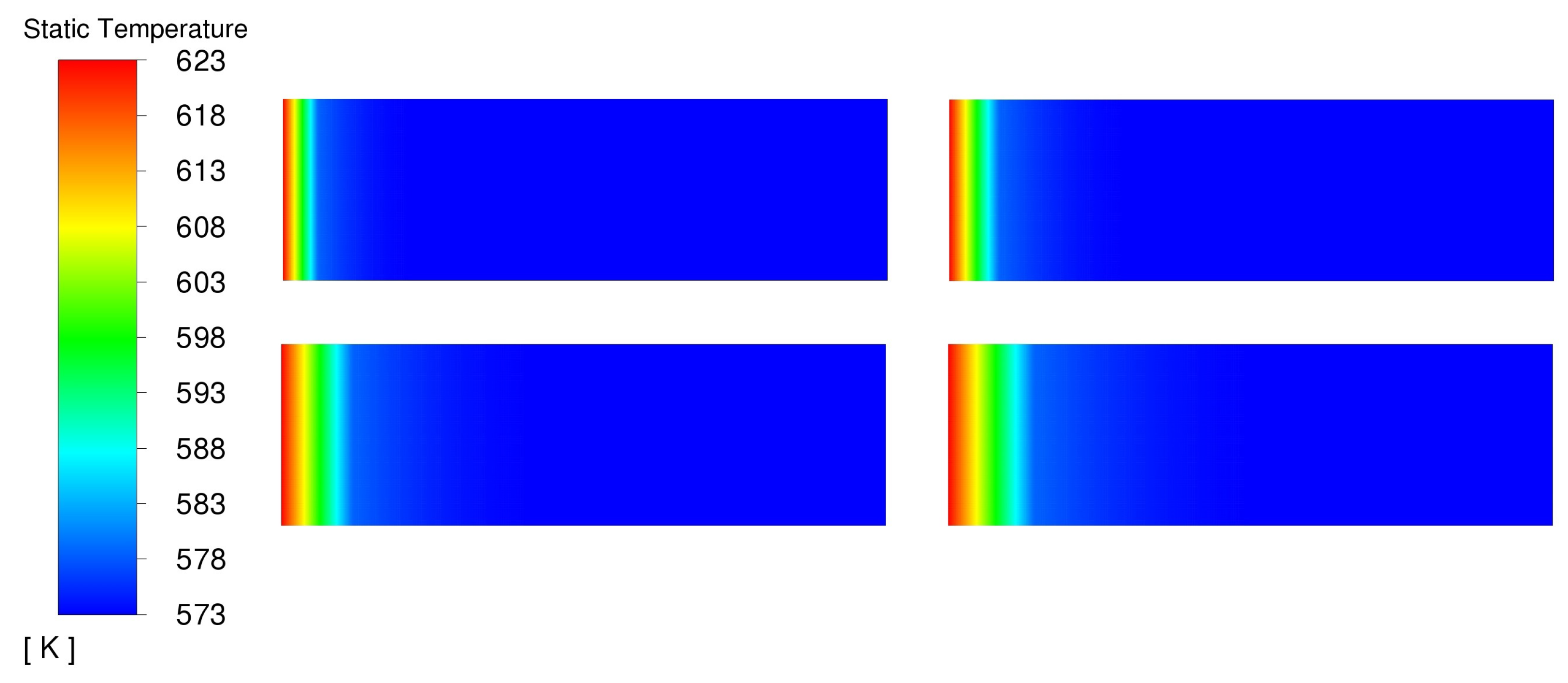
Figure 4.
Temperature contours at 5 min (top-left corner), 10 min (top-right corner), 20 min (bottom-left corner) and 30 min (bottom-right corner).
Figure 4.
Temperature contours at 5 min (top-left corner), 10 min (top-right corner), 20 min (bottom-left corner) and 30 min (bottom-right corner).

Figure 5.
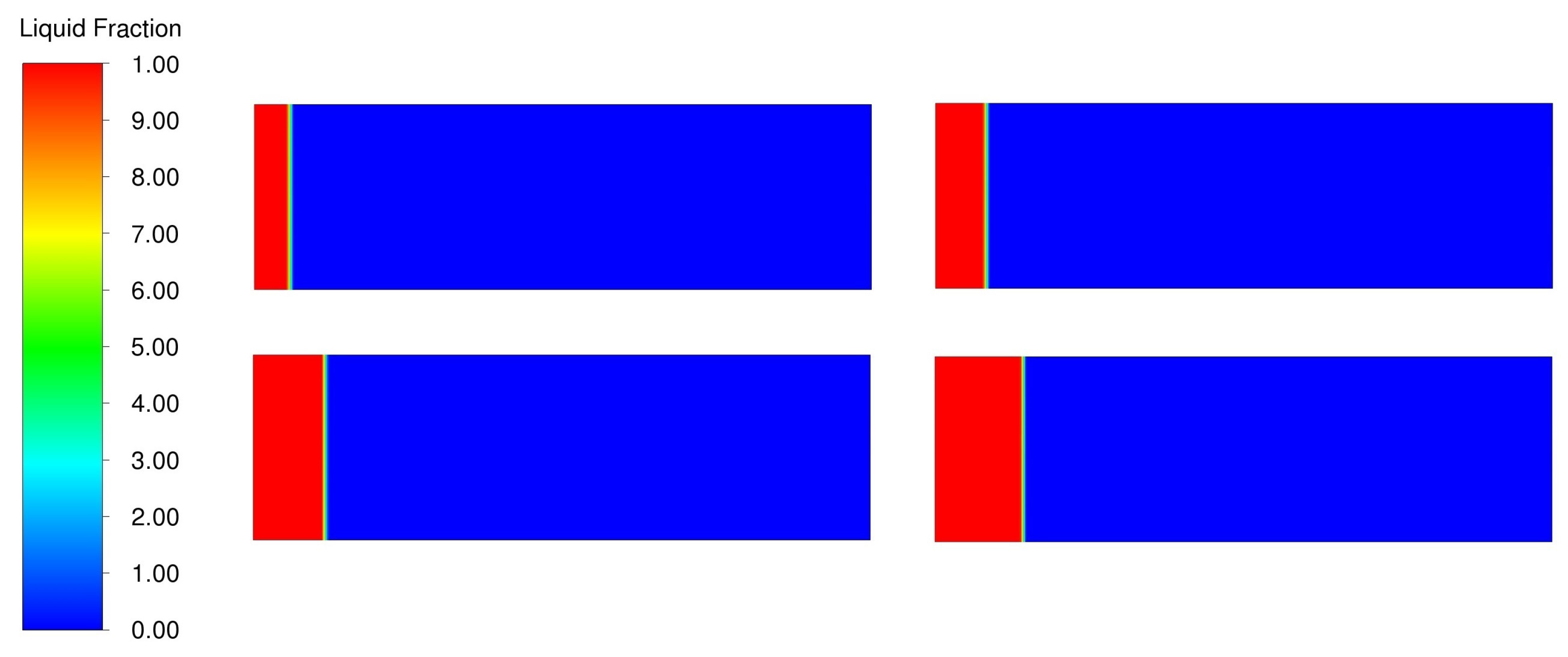
Liquid fraction contours at 5 min (top-left corner), 10 min (top-right corner), 20 min (bottom-left corner) and 30 min (bottom-right corner).
Figure 5.
Liquid fraction contours at 5 min (top-left corner), 10 min (top-right corner), 20 min (bottom-left corner) and 30 min (bottom-right corner).

Figure 6.
Temperature profiles at 5 min, 10 min, 20 min and 30 min.

Figure 7.
Detailed view of the maximum computational errors on the temperature field at 5 min, 10 min, 20 min and 30 min.
Figure 7.
Detailed view of the maximum computational errors on the temperature field at 5 min, 10 min, 20 min and 30 min.

Figure 8.
Melting frontier position over time for two-phase 1D Stefan problem.

Figure 9.
One of the three different geometries studied in the present work. It has a steel inner tube for heat transfer fluid flow (grey element) and an aluminium heat conduction structure connected to the heat transfer tube (green component). The PCM is all around the aluminium structure up to its outer radius.

Figure 10.
Simulated section of 9° for a model with 20 fins. It considers the fin’s half-thickness and the PCM area’s half-angle between two fins.
Figure 10.
Simulated section of 9° for a model with 20 fins. It considers the fin’s half-thickness and the PCM area’s half-angle between two fins.

Figure 11.
Simulated domains for the three axial structures under study: from left to right the rectangular, the trapezoidal and the fractal fin profiles.
Figure 11.
Simulated domains for the three axial structures under study: from left to right the rectangular, the trapezoidal and the fractal fin profiles.

Figure 12.
Temperature and liquid fraction contours for all the configurations at 5 min.

Figure 13.
Temperature and liquid fraction contours for all the configurations at 10 min.

Figure 14.
Temperature and liquid fraction contours for all the configurations at 15 min.

Figure 15.
Temperature and liquid fraction contours for all the configurations at 20 min.

Figure 16.
Temperature and liquid fraction contours for all the configurations at 30 min.

Figure 17.
Temperature and liquid fraction contours for all the configurations at 40 min.

Figure 18.
Temperature and liquid fraction contours for all the configurations at 50 min.

Figure 19.
Temperature and liquid fraction contours for all the configurations at 60 min.

Figure 20.
Temperature contours for the three configurations at the end of simulation time (t = 80 min).
Figure 20.
Temperature contours for the three configurations at the end of simulation time (t = 80 min).

Figure 21.
Total discharging power over time for the three configurations under study.

Figure 22.
Total discharging power over the state of charge for the three configurations under study.
Figure 22.
Total discharging power over the state of charge for the three configurations under study.


Table 1.
Thermo-physical properties of sodium nitrate (NaNO3), provided by the DLR Thermal Process Technology Department: is the density [ / ], c is the specific heat [ /( )], k is the thermal conductivity [ /( )], L is the enthalpy of phase change [ / ], is the melting temperature [ ].
Table 1.
Thermo-physical properties of sodium nitrate (NaNO3), provided by the DLR Thermal Process Technology Department: is the density [ / ], c is the specific heat [ /( )], k is the thermal conductivity [ /( )], L is the enthalpy of phase change [ / ], is the melting temperature [ ].
| NaNO3 | |||
|---|---|---|---|
| Symbol | Property | Solid | Liquid |
| Density | 2010.5 | 2010.5 | |
| c | Specific heat | 1655 | 1655 |
| k | Thermal conductivity | 0.56 | 0.56 |
| L | Enthalpy of phase change | - | 178,000 |
| Melting temperature | 306 | 306 | |
Table 2.
Maximum computational error on the temperature field and on the interface position at 5 min, 10 min, 20 min and 30 min.
Table 2.
Maximum computational error on the temperature field and on the interface position at 5 min, 10 min, 20 min and 30 min.
| Error | t = 5 min | t = 10 min | t = 20 min | t = 30 min |
|---|---|---|---|---|
| 1.16% | 1.09% | 1.93% | 1.03% | |
| 0.76% | 0.73% | 2.5% | 0.71% |
Table 3.
Constant parameters for the three configurations under study.
| Material | Characteristic Dimensions | ||
|---|---|---|---|
| Steel ring | 0.0063 | ||
| 0.0086 | |||
| area | 0.0001076616 | m2 | |
| Aluminium ring | 0.0086 | ||
| 0.0106 | |||
| Aluminium fins | number | 20 | |
| 0.0106 | |||
| 0.0525 | m | ||
| Total aluminium structure | area | 0.00091644 | m2 |
| PCM | 0.0106 | ||
| 0.0525 | |||
| area | 0.00751032 | m2 | |
Table 4.
Number of nodes and elements of the mesh for each configuration.
| Rectangular Fins | Trapezoidal Fins | Fractal Fins | |
|---|---|---|---|
| Nodes | 16,409 | 16,622 | 17,096 |
| Elements | 5308 | 5383 | 5543 |
Table 5.
Liquid fraction evolution over time for the three configurations under study.
| Rectangular Fins | Trapezoidal Fins | Fractal Fins | |
|---|---|---|---|
| 5 min | 76.16% | 75.00% | 75.94% |
| 10 min | 61.02% | 59.41% | 60.09% |
| 15 min | 48.87% | 47.09% | 46.90% |
| 20 min | 38.71% | 36.94% | 35.51% |
| 30 min | 22.74% | 21.26% | 16.21% |
| 40 min | 11.29% | 10.24% | 4.18% |
| 50 min | 3.62% | 3.01% | 0% |
| 60 min | 0% | 0% | 0% |
Table 6.
Average discharging power (for a time corresponding to LF = 10%), total energy from the enthalpy of phase change formula (at the end-of-the-simulation time) and total energy calculated from power (at the end-of-simulation time) for the three configurations under study.
Table 6.
Average discharging power (for a time corresponding to LF = 10%), total energy from the enthalpy of phase change formula (at the end-of-the-simulation time) and total energy calculated from power (at the end-of-simulation time) for the three configurations under study.
| Total Time | Rectangular Fins | Trapezoidal Fins | Fractal Fins | |
|---|---|---|---|---|
| t:LF = 10% | −950.8 W | −979.4 W | −1136.6 W | |
| 80 min | J | J | J | |
| 80 min | J | J | J |
Publisher’s Note: MDPI stays neutral with regard to jurisdictional claims in published maps and institutional affiliations. |
© 2022 by the authors. Licensee MDPI, Basel, Switzerland. This article is an open access article distributed under the terms and conditions of the Creative Commons Attribution (CC BY) license (https://creativecommons.org/licenses/by/4.0/).
Share and Cite
MDPI and ACS Style
Privitera, E.; Caponetto, R.; Matera, F.; Vasta, S. Impact of Geometry on a Thermal-Energy Storage Finned Tube during the Discharging Process. Energies 2022, 15, 7950. https://doi.org/10.3390/en15217950
AMA Style
Privitera E, Caponetto R, Matera F, Vasta S. Impact of Geometry on a Thermal-Energy Storage Finned Tube during the Discharging Process. Energies. 2022; 15(21):7950. https://doi.org/10.3390/en15217950
Chicago/Turabian StylePrivitera, Emanuela, Riccardo Caponetto, Fabio Matera, and Salvatore Vasta. 2022. "Impact of Geometry on a Thermal-Energy Storage Finned Tube during the Discharging Process" Energies 15, no. 21: 7950. https://doi.org/10.3390/en15217950
Note that from the first issue of 2016, this journal uses article numbers instead of page numbers. See further details here.