
High-Resolution Seismic Characterization of Gas Hydrate Reservoir Using Wave-Equation-Based Inversion
1
Key Laboratory of Petroleum Resource Research, Institute of Geology and Geophysics, Chinese Academy of Sciences, Beijing 100029, China
2
Innovation Academy for Earth Science, Chinese Academy of Sciences, Beijing 100029, China
*
Author to whom correspondence should be addressed.
Energies 2022, 15(20), 7652; https://doi.org/10.3390/en15207652
Submission received: 6 September 2022
/
Revised: 5 October 2022
/
Accepted: 12 October 2022
/
Published: 17 October 2022
(This article belongs to the Special Issue Characterization of Conventional and Unconventional Hydrocarbon Reservoirs)
Abstract
:The high-resolution seismic characterization of gas hydrate reservoirs plays an important role in the detection and exploration of gas hydrate. The conventional AVO (amplitude variation with offset) method is based on a linearized Zoeppritz equation and utilizes only the reflected wave for inversion. This reduces the accuracy and resolution of the inversion properties and results in incorrect reservoir interpretation. We have studied a high-resolution wave-equation-based inversion method for gas hydrate reservoirs. The inversion depends on the scattering integral wave equation that describes a nonlinear relationship between the seismic wavefield and the elastic properties of the subsurface medium. In addition to the reflected wave, it considers more wavefields including the multiple scattering and transmission during inversion to improve the subsurface illumination, so as to enhance the accuracy and resolution of the inversion properties. The results of synthetic data from Pearl River Mouth Basin, South China Sea, demonstrate the validity and advantages of the wave-equation-based inversion method. It can effectively improve the resolution of inversion results compared to the conventional AVO method. In addition, it has good performance in the presence of noise, which makes it a promising method for field data.
1. Introduction
Gas hydrate is an ice-like solid formed of water and gas. It is composed of a methane molecule enclosed within a crystalline structure of water molecules [1,2,3,4]. There is abundant methane in gas hydrate. The carbon stored in gas hydrate is about twice the total carbon content of all fossil fuels (including coal, oil, and natural gas) [5]. The advantages of gas hydrate make it a potential energy resource in the future. However, from the environmental aspects, the methane in gas hydrate is a powerful greenhouse gas. It is 20–30 times more potent at trapping heat in the atmosphere than carbon dioxide [6,7]. Climate and ocean warming may reduce the stability of gas hydrates, leading to hydrate dissociation and thus the release of methane into the ocean and overlying sediments. The released methane may eventually reach the atmosphere and aggravate the greenhouse effect [6]. Thus, gas hydrate reservoirs have a possible impact on climate change. The detection and exploration of gas hydrate reservoirs are important from both the energy and environmental perspective.
The occurrence of gas hydrate is controlled by the geological environment. Sufficient concentrations of methane are necessary to form the gas hydrate reservoir. The methane may be generated by biological activities in sediments, and it may also migrate from the organic matter at depth. Therefore, natural gas hydrate is most likely to be formed at locations wherein active upward fluid migration occurs, such as oceanic and lacustrine sediments [8]. In addition, gas hydrate in nature is usually found in areas with high pressure and low temperature, such as the seafloor and permafrost sediments. The pressure and temperature conditions in these areas can keep gas hydrate stable [9]. According to the geological environment and physical properties, the geological gas hydrate deposits can be categorized into five major types [10]. The regionally disseminated low-concentration hydrate is primarily found in mostly impermeable clays. In this case, methane hydrate fills pores and/or displaces sediment grains to form crystals or nodules from a few tens of meters below the seafloor to the base of the gas hydrate stability zone (GHSZ). The saturation of methane hydrate is less than ~10%. The fracture-filling hydrate is usually found in clay-dominated fracture sediments at non-vent sites. This type of hydrate is distributed at a shallow depth (e.g., 50–300 mbsf) below seafloor with a low-to-moderate saturation. In addition, the hydrate may be enriched at the base of the GHSZ in muddy sediments. The saturation of this type of hydrate commonly increases abruptly, with depth from the background value in the muddy sediments, to more than 10% near the base of the GHSZ. The fourth type is concentrated hydrate at vent sites. This type of hydrate may exist from near the seafloor to approximately 50 mbsf, or it may be as deep as ~160 mbsf. The saturation ranges from 40% to >90%. The final type is concentrated hydrate in sandy sediments. It may be found above the base of the GHSZ and is composed of gas hydrate in thin sandy or silty beds bounded by sandy sediments. It may also be found in thick sandy sediments that cross or near the base of the GHSZ.
Seismic technology plays an important role in the detection and exploration of gas hydrate reservoirs. Seismic data have been successfully applied in the identification of gas hydrate reservoirs together with other geophysical methods, including seismic facies analysis. Yoo et al. have studied multichannel seismic reflection and well-log data from the Ulleung Basin, East Sea [11]. These data have revealed several seismic features indicative of gas hydrate occurrence, including the bottom-simulating reflector (BSR), seismic chimneys, acoustic blanking, enhanced reflection below the BSR, and seafloor gas-escape features. The BSR is formed by a strong impedance contrast between the overlying sediments containing gas hydrate and the underlying sediments containing free gas [12,13]. It is usually parallel to the seafloor and has high amplitude and reversed polarity with respect to the seafloor reflection. However, the BSR does not necessarily translate into the existence of gas hydrate because it might be present in the sediments without gas hydrate [14]. Seismic chimneys are characterized by low-to-high, upward-bending internal reflections. The velocity inside the chimney is higher than that in the surrounding sediments, which is caused by the active migration of fluid gas into the GHSZ. The acoustic blanking in the seismic profile may be attributed to the energy attenuation due to the presence of free gas or the poor seismic energy penetration due to the strong reflection from a layer of gas hydrate. The enhanced reflection below the BSR is correlated with the strong impedance contrasts due to free gas accumulation below the BSR. When the upward-migrating gas escapes into the water column through the seafloor pockmarks and mud mounds, gas seepage at the seafloor can be found [15]. Riedel et al. have added an additional element into a regional assessment strategy of gas hydrate occurrence by including the depositional environment defined through seismic facies classes [16]. The seismic facies classification is attempted using regional 2D seismic data and a 3D seismic volume, as well as core and log data from two gas hydrate drilling expeditions carried out in the Ulleung Basin, East Sea, to conduct a fully integrated gas hydrate assessment. Wu et al. have analyzed the drilling results in the Shenhu Area, South China Sea [17]. In the case that free gas exists beneath hydrate deposits, the frequency of the hydrate deposits will be noticeably attenuated, with the attenuation degree mainly affected by pore development and free gas content. Thus, frequency can be used as an important seismic attribute to identify hydrate reservoirs. These parameters could indicate the occurrence of gas hydrate; however, they fail to quantify it.
Amplitude variation with offset (AVO) is a conventional technique for quantitative reservoir characterization [18,19]. It can predict the elastic parameters of formation (P-wave velocity, S-wave velocity, and density) from the seismic data. Then, the rock and fluid properties of the reservoir (lithology, porosity, permeability, and saturation) can be estimated from the predicted elastic parameters based on rock physics models. Chen et al. applied AVO inversion to calculate the P- and S-wave velocities and density and then to estimate the gas hydrate and free-gas concentrations above and below the BSR interface. The estimated gas hydrate and free-gas concentrations are at a 90% credibility level. The results indicate that this method cannot provide enough accuracy for resolving the gas hydrate and free-gas concentrations independently [20]. Ojha and Sain performed an amplitude versus angle (AVA) modeling of seismic data from a BSR to calculate the P- and S-wave velocities and then derived the saturation of gas hydrate with rock physics modeling. The results can help to understand the origin of BSR [21]. Zhang et al. performed AVO forward modeling and AVO attribute inversion to the seismic data from the Shenhu area [22]. Their results confirmed that the AVO attributes depend on the content of gas hydrate and free gas. However, most of the current AVO method only considers the reflected wave for inversion. It is built based on the approximation of the Zoeppritz equation [23,24]. The simplified equation indicates a linear relationship between the reflected wavefield and the contrast variables of P- and S-wave velocities and density (i.e., , , and ). In fact, the seismic wavefield is usually non-linear with respect to the elastic properties of the subsurface medium. Therefore, the conventional AVO method based on the linearized Zoeppritz equation reduces the accuracy and resolution of the inversion properties, resulting in incorrect reservoir interpretation.
Different methods have been proposed to improve the accuracy and resolution of the conventional seismic inversion method. Alemie and Sacchi proposed a high-resolution three-term AVO inversion by introducing a Trivariate Cauchy probability distribution. This distribution can model the prior distribution of the AVO parameters with sparsity, thus leading to a high-resolution estimate of subsurface models [25]. Zhang et al. introduced low-frequency information to improve the resolution [26]. Niu et al. proposed a data-driven method to improve the linear approximation of the conventional AVO inversion method. Well-logging data were used to correct the inaccurate linearized AVO operators. The results of synthetic and field data demonstrated that the accuracy and resolution of the inverted results were improved using the proposed method [24]. Yi et al. proposed a new method using stepwise seismic inversion and 3D seismic datasets with two different resolutions [27]. The proposed method can track a thin gas hydrate-bearing sand layer compared with the conventional seismic inversion method with a maximum resolution of ~10 m. The gas hydrate distribution around the UBGH2-6 well in Ulleung Basin was estimated successfully using their method.
In this study, we have studied a high-resolution seismic characterization of a gas hydrate reservoir using a wave-equation-based method. Besides the reflected wave, more wavefields including multiple scattering and transmission are considered in the inversion process. We first present theories of the wave-equation-based inversion method. Then, a synthetic model from Pearl River Mouth Basin, South China Sea, is used to demonstrate the performance of this method in the high-resolution seismic characterization of the gas hydrate reservoir. Finally, we discuss the obtained results and the advantages of this method and provide the conclusions.
2. Methods
2.1. The AVO Inversion Method
The conventional AVO (amplitude variation with offset) inversion method is based on the approximation of the Zoeppritz equation, which describes the change of reflected amplitude with incident angle. The Zoeppritz equation is derived for the case of two half-space media separated by a horizontal interface [28]. As we know, the half-space media can be characterized by three elastic properties, namely P-wave velocity (), S-wave velocity (), and density (). When an incident P-wave hits the interface, it is split into the reflected P- and S- waves and transmitted to the P- and S- waves. According to the Zoeppritz equation, the reflection and transmission coefficients are functions of the incident angle and the three elastic properties. Therefore, the elastic properties can be inverted from the observed reflection coefficient, which is the basis of the AVO inversion method. Considering the complexity of the Zoeppritz equation, some approximations are usually used to simplify the Zoeppritz equation and provide an intuitive understanding of the relationship between reflection amplitude and elastic properties. One of the commonly used approximations, the Aki and Richards approximation [28], is shown in Equation (1). It assumes that the perturbation in the elastic properties is small.
where , , , and represent the average , , , and incident angle, respectively, across the interface. , , and represent the change of , , and , respectively, across the interface. represents the ratio of to .
Equation (1) can be expressed in the following matrix form.
where represents the number of incident angles. As seen from Equation (2), it describes a linear relationship between the reflection coefficient and elastic properties. It can be rewritten as
where is the linear operator defined by Equation (2), the unknown elastic properties, and the input seismic data.
The objective function of the conventional AVO inversion method is built based on Equation (3) and is shown as follows:
The elastic properties are easily obtained by solving Equation (4) using the least squares algorithm.
As seen from Equation (2), the conventional AVO method is built based on the approximation of the Zoeppritz equation [23,24]. The simplified equation considers only the reflected wave for inversion. It indicates a linear relationship between the reflected wavefield and the contrast variables of P- and S-wave velocities and density (i.e., , , and , respectively). In fact, the seismic wavefield is usually non-linear with respect to the elastic properties of the subsurface medium. Therefore, the conventional AVO method based on the linearized Zoeppritz equation reduces the accuracy and resolution of the inversion properties, resulting in incorrect reservoir interpretation.
2.2. The Wave-Equation-Based Inversion Method
The wave-equation-based inversion is employed to realize the high-resolution seismic characterization of the gas hydrate reservoir [29]. Given an initial subsurface model, the wave-equation-based inversion method first simulates the seismic wavefields using the given model and updates the model from the differences between the simulated wavefields and real data. The seismic wavefields are simulated based on the scattering integral equation for elastic waves [30,31]. As we know, the three elastic properties, namely , , and , can be expressed in terms of the elastic moduli as follows:
where the compressibility is related to the bulk modulus as , and the shear compliance is related to the shear modulus as . Assuming that the smooth background medium (, , ) is known, the contrasts against the background (, , and ) are formulated as
Therefore, the scattering integral equation for elastic waves in the frequency domain is expressed by the contrast functions as
where represents the total seismic wavefield propagating in the true medium, and the incident wavefield propagating in the background medium. They are excited by a source at and recorded at each depth in the subsurface medium. The second term on the right of the equal sign in Equation (10) represents the scattered wavefield field. is the Green’s function. defines the objective domain of interest. and are pre-calculated using the known background medium. As seen from Equation (10), the relationship between the total seismic wavefield and the elastic properties of the subsurface medium is nonlinear. This nonlinearity indicates that multiple scattering and transmission are considered for the inversion of medium properties, not only the reflected wavefield. Therefore, the inversion method based on Equation (10) can improve the accuracy and resolution of the inversion properties compared with the conventional AVO method based on Equation (2). However, it has a higher computational cost.
According to Equation (10), the total wavefield is obtained once the contrast function is known. After the total wavefield is calculated, the seismic data recorded at the receiver are given as follows:
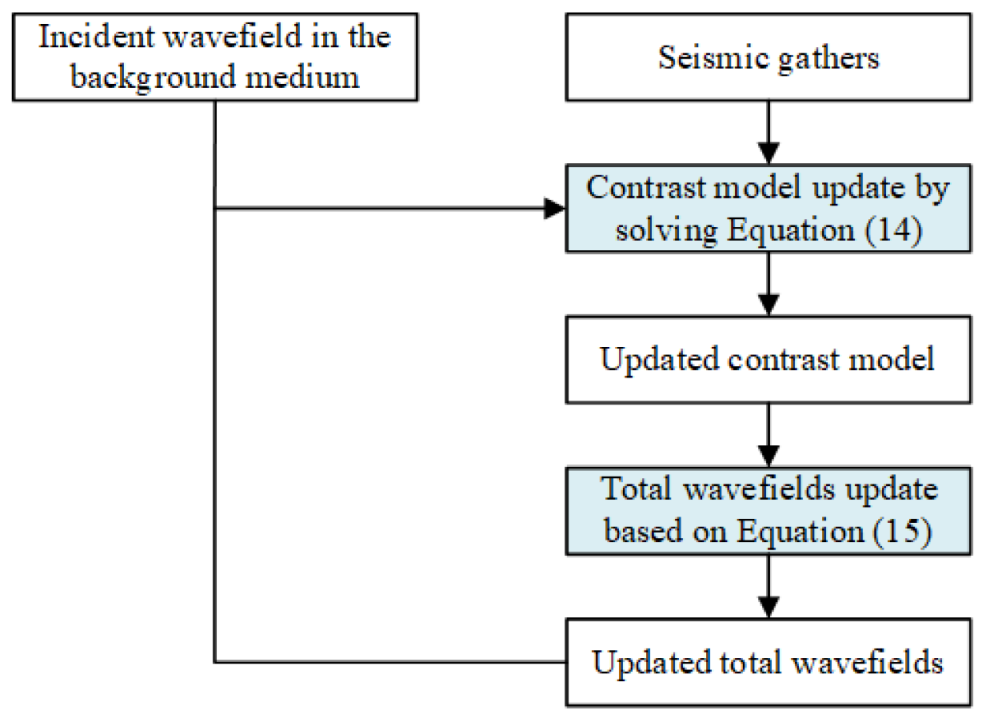
The wave-equation-based inversion scheme is built based on the above Equations (10) and (11), and is implemented in an iterative manner by alternately updating the contrast models with a current best knowledge of the total wavefield and then updating the total wavefield with a current contrast model. The objective function of the contrast model update is based on the misfit between actual and synthetic data and is shown as follows:
where is actual seismic data and is synthetic data calculated by Equation (11). The total wavefield in Equation (11) is the incident wavefield at the first iteration and fixed at the current best estimate in the subsequent iterations.
The inversion process defined by the objective function in Equation (12) is unstable because there are always some forms of noise in the actual seismic data. Therefore, a regularization term is introduced to stabilize the inversion process. There are many different regularization methods, such as Tikhonov regularization [32,33] and total variation (TV) regularization [34] et al. We use a Sobolev norm-based regularization [35,36] which is shown as follows:
Equation (13) becomes TV regularization when . It becomes Tikhonov regularization when . Therefore, the Sobolev norm-based regularization is a blend of the Tikhonov regularization and the TV regularization. In this study, we set to decrease gradually from 2 to 1 in a logarithmic decreasing manner during the inversion process. This can ensure the smoothness of the inverted models in the early iteration of inversion and preserve the boundary of the models in the later iteration.
The regularization term can be added in an additive and multiplicative manner. Compared with additive regularization, multiplicative regularization can avoid the selection of a regularization parameter that balances the data misfit and regularization term. Therefore, we select multiplicative regularization in this study. The final objective function is defined as:
Once the contrast model is updated, the total wavefield is updated based on Equation (10) by fixing the updated contrast model. However, the update of the total wavefield is not realized at one time. Instead, it is updated iteratively by a Krylov subspace method in Equation (15):
where is the weighting coefficient, and is the number of iterations. is the difference between two successive wavefields and is defined as follows [29]:
The weighing coefficients are solved when the calculated wavefields by Equations (10) and (16) fit well. One more order of scattering is added in each iteration of the wavefield update. All orders of scattering are considered until the last iteration in the inversion process.
After the total wavefields are updated, they are substituted into Equations (11) and (12) again to obtain an improved estimate of the contrast models. This process is iterated until the synthetic data fits well with the real data. Finally, characteristics (, , and ) of the subsurface media are obtained by substituting the inversion models into Equations (5) and (6). Figure 1 summarizes the workflow of the wave-equation-based inversion method. As shown in Figure 1, the models and total wavefield are updated iteratively in an alternating manner during the inversion process. The subsurface models are first updated given the initial background models. Then, the wavefield is updated based on the updated models. The two processes are repeated until the misfit between the real and synthetic seismic wavefield is small. The total wavefield is regarded as the summation of the background wavefield and scattering wavefield. One more order of scattering is considered at each iteration. As more order scattering fields are included, the inversion models become closer to the real models. Finally, the total wavefields used for inversion include all multiple scattering and transmission.
3. Synthetic Model and Data
A synthetic model from Pearl River Mouth Basin, South China Sea, is used to verify the wave-equation-based inversion method. In this section, we first present the geological setting in the studied area and introduce how the synthetic model and data were derived.
3.1. Geological Setting
The Pearl River Mouth Basin is located in the northern part of the South China Sea. The Baiyun Sag, located in the southern Pearl River Mouth basin, is the largest and deepest subbasin in the Pearl River Mouth Basin (Figure 2). It has a water depth of 200~2000 m and an area of more than 20,000 km2 [37,38,39]. The Baiyun Sag has experienced complex tectonic evolution, including rifting, depression, and fault block rise and fall. The depositional environment in the Baiyun Sag evolved gradually from continental into shallow marine and continental slope deep water facies and finally, substantial deep-water sediments were developed [40]. The formations from the base to top are the Wenchang Formation of Eocene, the Enping Formation and Zhuhai Formation of Oligocene, the Zhujiang Formation, the Hanjiang Formation, the Yuehai Formation of Miocene, the Wanshan Formation of Pliocene, and the Quaternary sediment [41,42,43]. The Wenchang Formation and the Enping Formation are the high-quality source rock that provide gas for the shallow gas hydrate deposits. The former is lacustrine sediment during the rifting period. The latter is lacustrine sediment during the fault-depression period. The Zhuhai Formation is a transitional deltaic deposit. It is composed of littoral sandy mudstone. The Zhujiang, Hanjiang, Yuehai, and Wanshan formations are shelf edge delta to slope-deep water deposits. They are composed of littoral mudstone, marine mudstone, and neritic sandstone and mudstone. These strata develop three sets of reservoir-cap assemblage. A large number of faults are developed in the study area. They migrate the deep gas to the shallow gas hydrate stable zones. Some thin gas hydrate reservoirs have been found in the shallow layer. They are distributed tens to hundreds of meters below the seabed.
3.2. Synthetic Model and Data
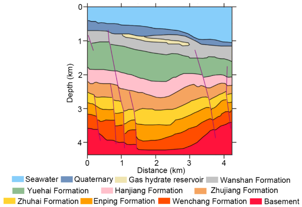
The geological structure of the Pearl River Mouth Basin has been investigated in detail [37,38,39,40,41,42,43] in previous studies. Several geological models have been published. We used a geological model (in Figure 3) [44] built based on the study of a 2D seismic line indicated by the red line in Figure 1. The horizontal and vertical intervals of the model are both 5 m. The seawater depth at this location is about 400~1000 m. As mentioned above, there are nine different strata below the sea floor defined by their sedimentary environment. A large number of faults are developed in the study area, indicated by the red lines in Figure 3. The gas hydrate reservoir was formed in the Wanshan Formation and lies at a depth of 800 m according to a bottom-simulating reflector in the seismic profile. The thickness of the gas hydrate reservoir is about 15 m.
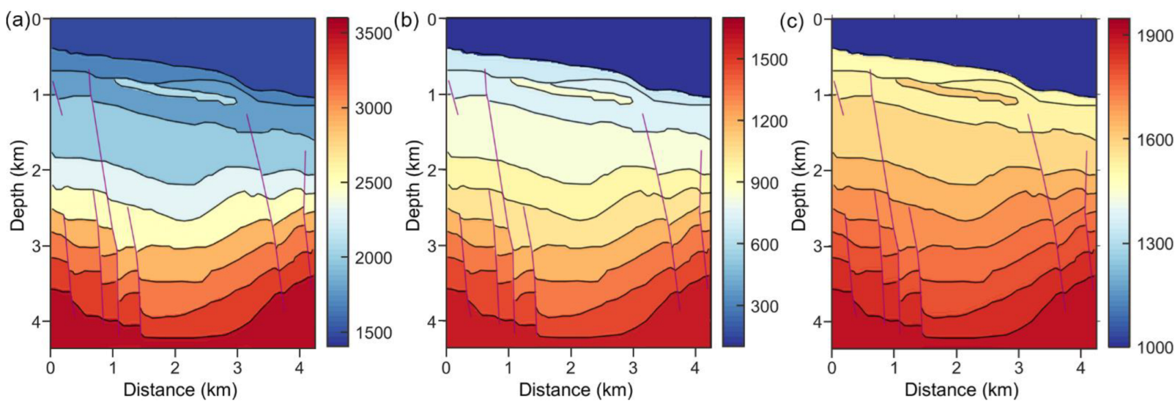
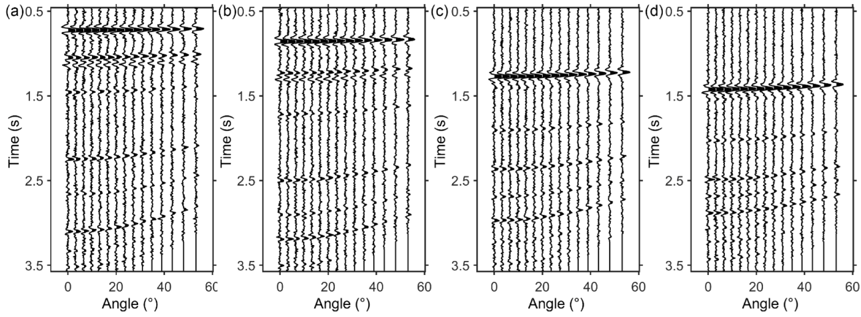
Based on the well log information and fine velocity modeling in the study area [45,46], the P-wave velocity (), S-wave velocity (), and density () are assigned to the geological model to simulate seismic wavefields, as shown in Figure 4. Then, seismic wavefields are modeled using the reflectivity method [47,48]. A total of 850 angle gathers are simulated. Figure 5 shows examples of obtained seismic angle gathers at 1.25 km, 2.25 km, 3.25 km, and 4.25 km.
4. Results
4.1. Inversion of the Synthetic Gas Hydrate Reservoir Model
To compare with the wave-equation-based inversion method, the conventional AVO inversion method is first applied to all the input gathers to invert the P-wave velocity, S-wave velocity, and density models. Then, the wave-equation-based inversion method is performed. The background models used in the conventional AVO inversion and the wave-equation-based inversion method are obtained by applying Gaussian smoothing to the real models in Figure 4. The stratigraphic horizons in the background models are almost unrecognizable, as shown in Figure 6.
Figure 7 shows the inverted P-wave velocity, S-wave velocity, and density models using the conventional AVO method. The stratigraphic horizons and faults indicated by the black and red lines in Figure 2 are added to the inverted models to compare with the true models in Figure 2. The black lines indicate the horizons and the red lines indicate the faults. As shown in Figure 7, the obtained models using the conventional AVO method are smooth and have a low resolution. The gas hydrate reservoir cannot be well identified from the inversion results. The inverted stratigraphic horizons indicated by the black arrows do not agree well with the real ones. Figure 8 compares the true models (red lines) with the inverted models (blue lines) at 2.25 km. As shown by the black arrows, it is difficult to identify the boundary of the gas hydrate reservoir, especially for the S-wave velocity and density models. The synthetic seismic angle gather after the final inversion at 2.25 km is shown in Figure 9a. It has a large error with the real seismic gather in Figure 5b, as shown in Figure 9b. This is because the conventional AVO inversion method only considers the reflected wavefield and a linear relationship between the reflected wavefield and the elastic properties of the subsurface medium, thus leading to lower accuracy and resolution.
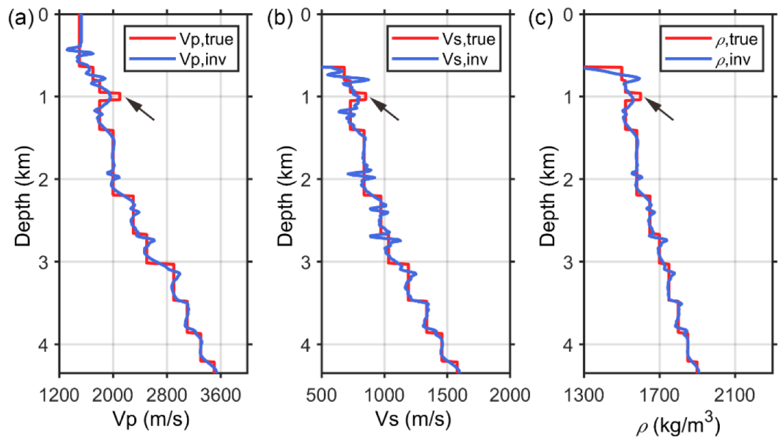
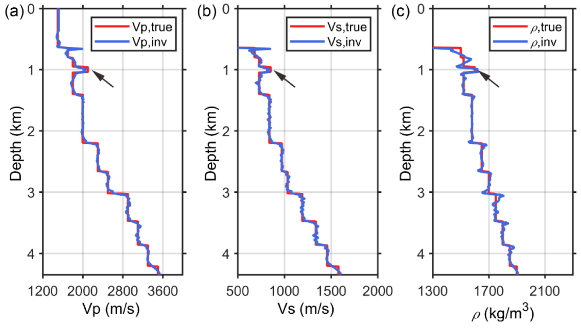
The inverted models using the wave-equation-based inversion method are shown in Figure 10. The gas hydrate reservoir is clearly reconstructed with high accuracy and resolution. More details are shown in the inverted models than in the conventional AVO inversion results in Figure 7. The inverted stratigraphic horizons agree well with the real ones. Figure 11 compares the true models (red lines) with the inverted models (blue lines) at 2.25 km. The inversion results are almost the same as the true models (red lines). The synthetic seismic angle gather for the final inverted models in Figure 12a exhibits a good agreement with the real seismic gather in Figure 5b. The error between the two gathers is small, as shown in Figure 12b. As described in the theory of the wave-equation-based method, the total wavefields including all multiple scattering and transmission are used for inversion. This contributes to improving the subsurface illumination by considering more wavefields. Therefore, the accuracy and resolution of the inversion results are improved.
4.2. Reliability Analysis for the Noisy Data
Due to the sensitivity to noise of inversion methods, the reliability analysis for the noisy data is studied to test the influence of noise on the inversion. The noisy seismic gathers are generated by adding Gaussian random noise. The signal-to-noise ratio of noisy gathers in Figure 13 is of 10 dB. Then, the wave-equation-based inversion method is applied to the noisy data. Figure 14 shows the final inverted 2D models. As seen from the results, the models are still well inverted in the presence of noise. The gas hydrate reservoir is easy to identify from the inverted models. The inverted stratigraphic horizons still agree well with the real ones. Figure 15 shows the true (red lines) and inverted (blue lines) models for the seismic angle gather at 2.25 km. The boundary of the gas hydrate reservoir is clearly characterized. The synthetic seismic angle gathers after the final inversion in Figure 16a are similar to the real seismic angle gather in Figure 5b. The noise in the input angle gather is not fitted, as shown in Figure 16b.
5. Conclusions
The high-resolution seismic characterization of gas hydrate reservoirs is important for the accurate evaluation of gas hydrate resources, especially for thin gas hydrate reservoirs. We have studied a wave-equation-based inversion method for gas hydrate reservoirs in this work. It is based on the scattering integral wave equation, and a Sobolev norm-based regularization is considered during the inversion. Compared to the conventional AVO method, the wave-equation-based inversion method can characterize the gas hydrate reservoir with high resolution by taking into account all the multiple scattering and transmission. The advantages of this method are validated by a synthetic model from Pearl River Mouth Basin, South China Sea. Thin gas hydrate reservoirs are distributed in the studied area. They are buried shallowly and distributed tens to hundreds of meters below the seabed. The results demonstrate that the wave-equation-based inversion method can provide a higher resolution and accuracy than the conventional AVO inversion method. It shows good performance in the presence of noise. This makes it a promising method for the accurate evaluation of gas hydrate resources, especially for thin gas hydrate reservoirs.
Author Contributions
Conceptualization, J.S. and Y.W. (Yibo Wang); methodology, J.S. and Y.W. (Yibo Wang); software, J.S. and Y.W. (Yibo Wang); validation, J.S. and Y.W. (Yibo Wang); data curation, H.Y.; writing—original draft preparation, J.S. and Y.W. (Yibo Wang); writing—review and editing, J.S., Y.W. (Yibo Wang), Y.W. (Yanfei Wang) and H.Y.; project administration, Y.W. (Yibo Wang); funding acquisition, Y.W. (Yibo Wang). All authors have read and agreed to the published version of the manuscript.
Funding
This research was funded by The Key Research Program of the Institute of Geology and Geophysics, CAS: IGGCAS-201903109.
Data Availability Statement
Not applicable.
Conflicts of Interest
The authors declare no conflict of interest.
References
- Hassanpouryouzband, A.; Joonaki, E.; Farahani, M.V.; Takeya, S.; Ruppel, C.; Yang, J.; English, N.J.; Schicks, J.M.; Edlmann, K.; Mehrabian, H.; et al. Gas hydrates in sustainable chemistry. Chem. Soc. Rev. 2020, 49, 5225–5309. [Google Scholar] [CrossRef]
- Demirbas, A. Methane from gas hydrates in the black sea. Energy Sources Part A Recovery Util. Environ. Eff. 2009, 32, 165–171. [Google Scholar] [CrossRef]
- Aregbe, A.G. Gas hydrate—Properties, formation and benefits. Open J. Yangtze Oil Gas 2017, 2, 27–44. [Google Scholar] [CrossRef] [Green Version]
- Chazallon, B.; Rodriguez, C.T.; Ruffine, L.; Carpentier, Y.; Donval, J.P.; Ker, S.; Riboulot, V. Characterizing the variability of natural gas hydrate composition from a selected site of the Western Black Sea, off Romania. Mar. Pet. Geol. 2021, 124, 104785. [Google Scholar] [CrossRef]
- Park, Y.; Kim, D.Y.; Lee, J.W.; Huh, D.G.; Park, K.P.; Lee, J.; Lee, H. Sequestering carbon dioxide into complex structures of naturally occurring gas hydrates. Proc. Natl. Acad. Sci. USA 2006, 103, 12690–12694. [Google Scholar] [CrossRef] [PubMed] [Green Version]
- Farahani, M.V.; Hassanpouryouzband, A.; Yang, J.; Tohidi, B. Insights into the climate-driven evolution of gas hydrate-bearing permafrost sediments: Implications for prediction of environmental impacts and security of energy in cold regions. RSC Adv. 2021, 11, 14334–14346. [Google Scholar] [CrossRef] [PubMed]
- Farahani, M.V.; Hassanpouryouzband, A.; Yang, J.; Tohidi, B. Development of a coupled geophysical–geothermal scheme for quantification of hydrates in gas hydrate-bearing permafrost sediments. Phys. Chem. Chem. Phys. 2021, 23, 24249–24264. [Google Scholar] [CrossRef]
- Hovland, M.; Gallagher, J.W.; Clennell, M.B.; Lekvam, K. Gas hydrate and free gas volumes in marine sediments: Example from the Niger Delta front. Mar. Pet. Geol. 1997, 14, 245–255. [Google Scholar] [CrossRef]
- Schicks, J.M. Gas hydrates in nature and in the laboratory: Necessary requirements for formation and properties of the resulting hydrate phase. ChemTexts 2022, 8, 13. [Google Scholar] [CrossRef]
- You, K.; Flemings, P.B.; Malinverno, A.; Collett, T.S.; Darnell, K. Mechanisms of methane hydrate formation in geological systems. Rev. Geophys. 2019, 57, 1146–1196. [Google Scholar] [CrossRef]
- Yoo, D.G.; Kang, N.K.; Yi, B.Y.; Kim, G.Y.; Ryu, B.J.; Lee, K.; Lee, G.H.; Riedel, M. Occurrence and seismic characteristics of gas hydrate in the Ulleung Basin, East Sea. Mar. Pet. Geol. 2013, 47, 236–247. [Google Scholar] [CrossRef]
- Mosher, D.C. A margin-wide BSR gas hydrate assessment: Canada’s Atlantic margin. Mar. Pet. Geol. 2011, 28, 1540–1553. [Google Scholar] [CrossRef]
- Madrussani, G.; Rossi, G.; Camerlenghi, A. Gas hydrates, free gas distribution and fault pattern on the west Svalbard continental margin. Geophys. J. Int. 2010, 180, 666–684. [Google Scholar] [CrossRef]
- Ker, S.; Thomas, Y.; Riboulot, V.; Sultan, N.; Bernard, C.; Scalabrin, C.; Ion, G.; Marsset, B. Anomalously deep BSR related to a transient state of the gas hydrate system in the western Black Sea. Geochem. Geophys. Geosyst. 2019, 20, 442–459. [Google Scholar] [CrossRef] [Green Version]
- Hovland, M.; Svensen, H. Submarine pingoes: Indicators of shallow gas hydrates in a pockmark at Nyegga, Norwegian Sea. Mar. Geol. 2006, 228, 15–23. [Google Scholar] [CrossRef]
- Riedel, M.; Bahk, J.J.; Kim, H.S.; Yoo, D.G.; Kim, W.S.; Ryu, B.J. Seismic facies analyses as aid in regional gas hydrate assessments. Part-I: Classification analyses. Mar. Pet. Geol. 2013, 47, 248–268. [Google Scholar] [CrossRef]
- Wu, S.Y.; Liu, J.; Xu, H.N.; Liu, C.L.; Ning, F.L.; Chu, H.X.; Wu, H.R.; Wang, K. Application of frequency division inversion in the prediction of heterogeneous natural gas hydrates reservoirs in the Shenhu Area, South China Sea. China Geol. 2022, 5, 251–266. [Google Scholar] [CrossRef]
- Hampson, D. AVO inversion, theory and practice. Lead. Edge 1991, 10, 39–42. [Google Scholar] [CrossRef]
- Buland, A.; Omre, H. Bayesian linearized AVO inversion. Geophysics 2003, 68, 185–198. [Google Scholar] [CrossRef] [Green Version]
- Chen MA, P.; Riedel, M.; Hyndman, R.D.; Dosso, S.E. AVO inversion of BSRs in marine gas hydrate studies. Geophysics 2007, 72, C31–C43. [Google Scholar] [CrossRef]
- Ojha, M.; Sain, K. Seismic velocities and quantification of gas-hydrates from AVA modeling in the western continental margin of India. Mar. Geophys. Res. 2007, 28, 101–107. [Google Scholar] [CrossRef]
- Zhang, X.; Yin, C.; Zhang, G. Confirmation of AVO Attribute Inversion Methods for Gas Hydrate Characteristics Using Drilling Results from the Shenhu Area, South China Sea. Pure Appl. Geophys. 2021, 178, 477–490. [Google Scholar] [CrossRef]
- Wang, Y. Approximations to the Zoeppritz equations and their use in AVO analysis. Geophysics 1999, 64, 1920–1927. [Google Scholar] [CrossRef] [Green Version]
- Niu, L.; Geng, J.; Wu, X.; Zhao, L.X.; Zhang, H. Data-driven method for an improved linearised AVO inversion. J. Geophys. Eng. 2021, 18, 1–22. [Google Scholar] [CrossRef]
- Alemie, W.; Sacchi, M.D. High-resolution three-term AVO inversion by means of a Trivariate Cauchy probability distribution. Geophysics 2011, 76, R43–R55. [Google Scholar] [CrossRef]
- Zhang, Y.P.; Zhou, H.; Zhang, M.Z.; Yu, B.; Wang, L.Q. High-resolution AVO inversion based on low-frequency information constraint. In SEG Technical Program Expanded Abstracts 2019; Society of Exploration Geophysicists: Houston, TX, USA, 2019; pp. 714–718. [Google Scholar]
- Yi, B.Y.; Yoon, Y.H.; Kim, Y.J.; Kim, G.Y.; Joo, Y.H.; Kang, N.K.; Kim, J.K.; Chun, J.H.; Yoo, D.G. Characterization of thin gas hydrate reservoir in ulleung basin with stepwise seismic inversion. Energies 2021, 14, 4077. [Google Scholar] [CrossRef]
- Aki, K.; Richards, P.G. Quantitative Seismology: Theory and Methods; WH Freeman and Co.: New York, NY, USA, 1980. [Google Scholar]
- Gisolf, D.; Haffinger, P.R.; Doulgeris, P. Reservoir-oriented wave-equation-based seismic amplitude variation with offset inversion. Interpretation 2017, 5, SL43–SL56. [Google Scholar] [CrossRef]
- Yang, J.Q.; Abubakar, A.; van den Berg, P.M.; Habashy, T.M.; Reitich, F. A CG-FFT approach to the solution of a stress-velocity formulation of three-dimensional elastic scattering problems. J. Comput. Phys. 2008, 227, 10018–10039. [Google Scholar] [CrossRef]
- Noor, M.A.; Noor, K.I.; Al-Said, E. New iterative methods for solving integral equations. Int. J. Mod. Phys. B 2011, 25, 4655–4660. [Google Scholar] [CrossRef]
- Golub, G.H.; Hansen, P.C.; O’Leary, D.P. Tikhonov regularization and total least squares. SIAM J. Matrix Anal. Appl. 1999, 21, 185–194. [Google Scholar] [CrossRef]
- Borsdorff, T.; Hasekamp, O.P.; Wassmann, A.; Landgraf, J. Insights into Tikhonov regularization: Application to trace gas column retrieval and the efficient calculation of total column averaging kernels. Atmos. Meas. Tech. 2014, 7, 523–535. [Google Scholar] [CrossRef] [Green Version]
- Strong, D.; Chan, T. Edge-preserving and scale-dependent properties of total variation regularization. Inverse Probl. 2003, 19, S165. [Google Scholar] [CrossRef]
- Hu, W.; Abubakar, A.; Habashy, T.M. Simultaneous multifrequency inversion of full-waveform seismic data. Geophysics 2009, 74, R1–R14. [Google Scholar] [CrossRef]
- Brezis, H.; Van Schaftingen, J.; Yung, P.L. A surprising formula for Sobolev norms. Proc. Natl. Acad. Sci. USA 2021, 118, e2025254118. [Google Scholar] [CrossRef]
- Wu, N.Y.; Zhang, H.Q.; Yang, S.X.; Zhang, G.X.; Liang, J.Q.; Lu, J.A.; Su, X.; Schultheiss, P.; Holland, M.; Zhu, Y.H. Gas Hydrate System of Shenhu Area, Northern South China Sea: Geochemical Results. J. Geol. Res. 2011, 2011, 370298. [Google Scholar] [CrossRef] [Green Version]
- Liu, C.L.; Ye, Y.G.; Meng, Q.G.; He, X.G.; Lu, H.L.; Zhang, J.; Liu, J.; Yang, S.X. The characteristics of gas hydrates recovered from Shenhu Area in the South China Sea. Mar. Geol. 2012, 307, 22–27. [Google Scholar] [CrossRef]
- Liang, J.; Meng, M.M.; Liang, J.Q.; Ren, J.F.; He, Y.L.; Li, T.W.; Xu, M.J.; Wang, X.X. Drilling Cores and Geophysical Characteristics of Gas Hydrate-Bearing Sediments in the Production Test Region in the Shenhu sea, South China sea. Front. Earth Sci. 2022, 10, 911123. [Google Scholar] [CrossRef]
- Pang, X.; Ren, J.Y.; Zheng, J.Y.; Liu, J.; Peng, Y.; Liu, B.J. Petroleum geology controlled by extensive detachment thinning of continental margin crust: A case study of Baiyun sag in the deep-water area of northern South China Sea. Pet. Explor. Dev. 2018, 45, 29–42. [Google Scholar] [CrossRef]
- Chen, D.X.; Wu, S.G.; Dong, D.D.; Mi, L.J.; Fu, S.Y.; Shi, H.S. Focused fluid flow in the Baiyun Sag, northern South China Sea: Implications for the source of gas in hydrate reservoirs. Chin. J. Oceanol. Limnol. 2013, 31, 178–189. [Google Scholar] [CrossRef]
- Lin, H.; Shi, H. Hydrocarbon accumulation conditions and exploration direction of Baiyun–Liwan deep water areas in the Pearl River Mouth Basin. Nat. Gas Ind. B 2014, 1, 150–158. [Google Scholar] [CrossRef]
- Gao, G.; Gang, W.; Zhang, G.; He, W.; Cui, X.; Shen, H.; Miao, S. Physical simulation of gas reservoir formation in the Liwan 3-1 deep-water gas field in the Baiyun sag, Pearl River Mouth Basin. Nat. Gas Ind. B 2015, 2, 77–87. [Google Scholar] [CrossRef]
- Su, P.B.; Liang, J.Q.; Sha, Z.B.; Fu, S.Y.; Lei, H.Y.; Gong, Y.H. Dynamic simulation of gas hydrate reservoirs in the Shenhu area, the northern South China Sea. Acta Pet. Sin. 2011, 32, 226. [Google Scholar]
- Liang, J.; Wang, M.J.; Lu, J.A.; Liang, J.Q.; Wang, H.B.; Kuang, Z.G. Characteristics of sonic and seismic velocities of gas hydrate bearing sediments in the Shenhu area, northern South China Sea. Nat. Gas Ind. 2013, 33, 29–35. [Google Scholar]
- Xue, H.; Du, M.; Wen, P.F.; Zhang, R.W.; Xu, Y.X.; Chen, X. Research and application of fine velocity modeling to gas hydrate testing development in the Shenhu area of South China Sea. Mar. Geol. Front. 2019, 35, 8–17. [Google Scholar]
- Kennett, B.L.N. Seismic Wave Propagation in Stratified Media; Cambridge University Press: Cambridge, UK, 1983. [Google Scholar]
- Mavko, G.; Mukerji, T.; Dvorkin, J. The Rock Physics Handbook; Cambridge University Press: Cambridge, UK, 1998. [Google Scholar]
Figure 1.
Workflow of the wave-equation-based inversion method.

Figure 2.
Location of the studied area. The red line indicates the location of the 2D seismic line that was used to build the geological model in Figure 3.
Figure 2.
Location of the studied area. The red line indicates the location of the 2D seismic line that was used to build the geological model in Figure 3.

Figure 3.
The geological model for synthetic data analysis. The black lines indicate the stratigraphic horizons and the red lines indicate the faults.
Figure 3.
The geological model for synthetic data analysis. The black lines indicate the stratigraphic horizons and the red lines indicate the faults.

Figure 4.
The true models for the synthetic data: (a) P-wave velocity, (b) S-wave velocity, and (c) density. The black lines indicate the stratigraphic horizons and the red lines indicate the faults.
Figure 4.
The true models for the synthetic data: (a) P-wave velocity, (b) S-wave velocity, and (c) density. The black lines indicate the stratigraphic horizons and the red lines indicate the faults.

Figure 5.
The noise-free seismic angle gathers at (a) 1.25 km, (b) 2.25 km, (c) 3.25 km, and (d) 4.25 km of the model.
Figure 5.
The noise-free seismic angle gathers at (a) 1.25 km, (b) 2.25 km, (c) 3.25 km, and (d) 4.25 km of the model.

Figure 6.
The background models used in the inversion method: (a) P-wave velocity, (b) S-wave velocity, and (c) density. The black lines indicate the stratigraphic horizons and the red lines indicate the faults.
Figure 6.
The background models used in the inversion method: (a) P-wave velocity, (b) S-wave velocity, and (c) density. The black lines indicate the stratigraphic horizons and the red lines indicate the faults.

Figure 7.
The inverted models from the noise-free data using the conventional AVO method: (a) P-wave velocity, (b) S-wave velocity, and (c) density. The black lines indicate the stratigraphic horizons and the red lines indicate the faults. The inverted stratigraphic horizons indicated by the black arrows do not agree well with the real ones.

Figure 8.
Comparison between the true model at 2.25 km and the inverted model from the noise-free data using the conventional AVO method: (a) P-wave velocity, (b) S-wave velocity, and (c) density. The black arrow indicates the location of the gas hydrate reservoir.
Figure 8.
Comparison between the true model at 2.25 km and the inverted model from the noise-free data using the conventional AVO method: (a) P-wave velocity, (b) S-wave velocity, and (c) density. The black arrow indicates the location of the gas hydrate reservoir.

Figure 9.
(a) Synthetic seismic angle gather at 2.25 km after the conventional AVO method, (b) difference between the real seismic gather in Figure 5b and synthetic seismic gather in (a).
Figure 9.
(a) Synthetic seismic angle gather at 2.25 km after the conventional AVO method, (b) difference between the real seismic gather in Figure 5b and synthetic seismic gather in (a).

Figure 10.
The inverted models from the noise-free data using the wave-equation-based inversion method: (a) P-wave velocity, (b) S-wave velocity, and (c) density. The black lines indicate the stratigraphic horizons and the red lines indicate the faults.
Figure 10.
The inverted models from the noise-free data using the wave-equation-based inversion method: (a) P-wave velocity, (b) S-wave velocity, and (c) density. The black lines indicate the stratigraphic horizons and the red lines indicate the faults.

Figure 11.
Comparison between the true model at 2.25 km and the inverted model from the noise-free data using the wave-equation-based inversion method: (a) P-wave velocity, (b) S-wave velocity, and (c) density. The black arrow indicates the location of the gas hydrate reservoir.
Figure 11.
Comparison between the true model at 2.25 km and the inverted model from the noise-free data using the wave-equation-based inversion method: (a) P-wave velocity, (b) S-wave velocity, and (c) density. The black arrow indicates the location of the gas hydrate reservoir.

Figure 12.
(a) Synthetic seismic angle gathers at 2.25 km after the wave-equation-based inversion method, (b) difference between the real seismic gather in Figure 3b and synthetic seismic gather in (a).
Figure 12.
(a) Synthetic seismic angle gathers at 2.25 km after the wave-equation-based inversion method, (b) difference between the real seismic gather in Figure 3b and synthetic seismic gather in (a).

Figure 13.
The noisy seismic angle gathers at (a) 1.25 km, (b) 2.25 km, (c) 3.25 km, and (d) 4.25 km of the model.
Figure 13.
The noisy seismic angle gathers at (a) 1.25 km, (b) 2.25 km, (c) 3.25 km, and (d) 4.25 km of the model.

Figure 14.
The inverted models from the noisy data using the wave-equation-based inversion method: (a) P-wave velocity, (b) S-wave velocity, and (c) density. The black lines indicate the stratigraphic horizons and the red lines indicate the faults.
Figure 14.
The inverted models from the noisy data using the wave-equation-based inversion method: (a) P-wave velocity, (b) S-wave velocity, and (c) density. The black lines indicate the stratigraphic horizons and the red lines indicate the faults.

Figure 15.
Comparison between the true model at 2.25 km and the inverted model from the noisy data using the wave-equation-based inversion method: (a) P-wave velocity, (b) S-wave velocity, and (c) density. The black arrow indicates the location of the gas hydrate reservoir.
Figure 15.
Comparison between the true model at 2.25 km and the inverted model from the noisy data using the wave-equation-based inversion method: (a) P-wave velocity, (b) S-wave velocity, and (c) density. The black arrow indicates the location of the gas hydrate reservoir.

Figure 16.
(a) Synthetic seismic angle gathers at 2.25 km after the wave-equation-based inversion method, (b) difference between the real seismic gather in Figure 10b and synthetic seismic gather in (a).
Figure 16.
(a) Synthetic seismic angle gathers at 2.25 km after the wave-equation-based inversion method, (b) difference between the real seismic gather in Figure 10b and synthetic seismic gather in (a).

Publisher’s Note: MDPI stays neutral with regard to jurisdictional claims in published maps and institutional affiliations. |
© 2022 by the authors. Licensee MDPI, Basel, Switzerland. This article is an open access article distributed under the terms and conditions of the Creative Commons Attribution (CC BY) license (https://creativecommons.org/licenses/by/4.0/).
Share and Cite
MDPI and ACS Style
Shao, J.; Wang, Y.; Wang, Y.; Yan, H. High-Resolution Seismic Characterization of Gas Hydrate Reservoir Using Wave-Equation-Based Inversion. Energies 2022, 15, 7652. https://doi.org/10.3390/en15207652
AMA Style
Shao J, Wang Y, Wang Y, Yan H. High-Resolution Seismic Characterization of Gas Hydrate Reservoir Using Wave-Equation-Based Inversion. Energies. 2022; 15(20):7652. https://doi.org/10.3390/en15207652
Chicago/Turabian StyleShao, Jie, Yibo Wang, Yanfei Wang, and Hongyong Yan. 2022. "High-Resolution Seismic Characterization of Gas Hydrate Reservoir Using Wave-Equation-Based Inversion" Energies 15, no. 20: 7652. https://doi.org/10.3390/en15207652
Note that from the first issue of 2016, this journal uses article numbers instead of page numbers. See further details here.