Simulation of Two-Phase Flow and Syngas Generation in Biomass Gasifier Based on Two-Fluid Model

Abstract

The efficient use of renewable energy is receiving more and more attention in the context of “carbon neutrality” and “carbon peaking”. For a long time, biomass has been used less efficiently as a renewable energy source, but with the development of fluidized biomass gasification technology, it can play an increasing role in industrial production. A fluidized bed biomass gasifier has a strong nonstationary process due to its complex energy–mass exchange, and analysis of its complex reaction process and products has relied on experiments for a long time. This paper uses a Euler–Euler two-fluid model to establish a three-dimensional CFD model of the fluidized bed biomass gasifier, on which factors affecting syngas generation are analyzed. The simulation shows that increasing the initial bed temperature can effectively improve syngas production, while increasing the air equivalent is not beneficial for syngas production.

1. Introduction

With the development of China’s economy and society, as a responsible major country in the international community, China has taken the initiative to commit to peak carbon emissions in 2035, which poses a huge challenge to China’s long-term energy supply situation, with coal currently the main energy source [1]. For a long time, the burning of coal has severely tested the environment, especially air quality. With the increasing attention on renewable energy, renewable clean energy sources such as solar, wind, tidal, and biomass have attracted more and more attention. In addition, the biomass produced in the process of agricultural and forestry production has been used by direct combustion for a long time, resulting in high pollution and low energy utilization efficiency. With the development of pyrolysis gasification technology, the efficient utilization of biomass energy can play an increasingly important role in energy supply.

Biomass gasification can use a spouted bed reactor, fluidized bed reactor, auger reactor, cyclone reactor, or rotating cone reactor. In these reactors, fluidized bed gasification technology has been widely used in biomass gasification because of its advantages of large capacity, high carbon conversion, and high syngas efficiency. Whereas fluidized bed gasifiers have a strong nonstationary process due to their complex energy–mass exchange and complex reaction process, syngas generation in gasifiers is affected by many factors. Only by studying their internal process deeply and understanding the process mechanism can gasification efficiency be further improved and energy consumption reduced. In order to study the flow and reactions of different substances in different types of gasifiers, a large number of experiments have been carried out [2,3,4,5,6]. However, the cost of running experiments is high, and experimental conditions are difficult to adjust accurately. For sensitivity analysis of some operating parameters, it takes a lot of time to carry out a series of experiments. Numerical simulation plays an important role in the study of gasifiers. There are two numerical simulation methods for gas–solid flow reactions in fluidized bed reactors: the Euler–Euler model and Euler–Lagrange model. The Euler–Lagrange model, in which each solid particle is tracked separately, requires a large amount of computation and is mainly used to calculate laboratory-scale fluidized bed reactors. The Euler–Euler model, on the other hand, considers solid particles as fluid and has a relatively small amount of calculation. Since Ding and Gidaspow [7] successfully applied particle dynamics (KTGF) theory to gas–solid flow in a bubbling fluidized bed in 1990, this method has become an important means to study dense gas–solid flow. Lathouwers and Bellan introduced chemical reactions and heat and mass transfer into this method and studied biomass pyrolysis in fluidized beds [8,9]. In recent years, application of the two-fluid model (TFM) based on particle dynamics theory in the coupling of dense gas–solid fluidization and chemical reaction has been widely studied [10,11,12,13].

An accurate CFD model is of great significance for optimization research of gasifiers. By changing the operating conditions and carrying out a series of simulation calculations, experimental cost can be greatly reduced and optimal operating conditions can be obtained. Ahmad et al. [14] used two different simulation softwares to parametrically analyze the factors that affect gasifier efficiency. Tang et al. [15] simulated the thermal characteristics of natural coke gasification in a fluidized bed. Their numerical results were in good agreement with the experimental results reported in the literature, which makes the developed models applicable for the design, optimization, and enlargement of gasifiers. Loha et al. [16] evaluated and compared the Euler–Euler and Euler–Lagrange models for a fluidized bed gasifier. Yang [17,18] used the core–annulus chamber model and the Lagrangian-based MP-PIC method to study the flow and reaction characteristics in a fluidized bed reaction system. Tamer [19] studied a pilot-scale gasifier in an oxygen-enriched environment and analyzed the syngas components under different conditions using a homemade CFD model; through comparison with experimental results, the model was proven to have good prediction ability.

Although there have been a lot of simulation studies on fluidized bed gasifiers, they mainly focus on the formation of syngas in gasifier. Research on gas–solid two-phase flow characteristics in gasifiers lacks adequate detail, and the complex gas–solid two-phase flow heat transfer in fluidized beds has great influence on the reaction. In this paper, a gas–solid flow reaction model based on Euler–Euler was established to describe the distribution of the gas–solid flow field and complex chemical reaction in the gasifier reactor. The bed material and biomass fuel particles were considered as a continuous medium for calculations. The change of flow heat transfer and chemical reaction components in gasifiers under different temperatures and excess air coefficient was simulated to analyze the influence of each factor on the syngas component of gasifiers.

2. Gas–Solid Flow and Reaction

2.1. Gas–Solid Flow Model

The continuity equations of two phases are as follows:

$$\frac{\partial }{\partial t}\left({\alpha }_g{\rho }_g\right)+\nabla \cdot \left({\alpha }_g{\rho }_g{u}_g\right)=S_{msg}$$

(1)

$$\frac{\partial }{\partial t}\left({\alpha }_s{\rho }_s\right)+\nabla \cdot \left({\alpha }_s{\rho }_s{u}_s\right)=S_{mgs}$$

(2)

where $\alpha$, $\rho$, and $u$ are the volume fraction, density, and velocity vectors of the gas–solid phase, respectively, with subscripts g for the gas phase and s for the solid phase.

$S_{mgs}=-S_{msg}$ represents the mass change of the gas–solid phase due to chemical reaction.

In this paper, the Mach number of the gas is far less than 1, and the gas phase pressure changes very little, so it can be simplified as an incompressible ideal gas.

In gas–solid flow, the forces of the particle phase include gravity, buoyancy, gas–solid drag, and pressure gradient between particle phases. In this paper, the buoyancy of the granular phase is ignored, and only interphase drag force, gravity, and pressure gradient are considered. The momentum equation of the gas–solid phase is:

$$\frac{\partial }{\partial t}\left({\alpha }_g{\rho }_g{u}_g\right)+\nabla \cdot \left({\alpha }_g{\rho }_g{u}_g{u}_g\right)=-{\alpha }_g\nabla p+{\alpha }_g{\rho }_{g}g+\nabla \cdot {\tau }_g-\beta \left(u_g-u_s\right)+{\mathrm{S}}_{vsg}$$

(3)

$$\frac{\partial }{\partial t}\left({\alpha }_s{\rho }_s{u}_s\right)+\nabla \cdot \left({\alpha }_s{\rho }_s{u}_s{u}_s\right)=-{\alpha }_s\nabla p+{\alpha }_s{\rho }_{s}g+\nabla \cdot {\tau }_s+\beta \left(u_g-u_s\right)+{\mathrm{S}}_{vgs}$$

(4)

where ${\tau }_g$ and ${\tau }_s$ are the corresponding force tensors of the two phases, $\beta$ is the drag coefficient, and $S_{vgs}$ is the momentum change caused by the mass change.

$${\tau }_g={\mu }_g\left[\nabla u_g+{\left(\nabla u_g\right)}^{\mathrm{T}}\right]-2{\mu }_g\left(\nabla \cdot u_g\right)I/3$$

(5)

$${\mu }_g={\mu }_{gt}+{\mu }_{gl}$$

(6)

$${\mu }_{gt}={\rho }_g{C}_{\mu }\frac{k_g^2}{{\epsilon }_g}$$

(7)

In this paper, the classical $k-\epsilon$ model is used to calculate turbulence. In order to simulate the dense gas–solid flow in a fluidized bed in detail, gas–solid two-phase flow is calculated using an individual phase-turbulence model. Both gas and solid phases are treated as quasi-fluids, and the governing equations are the same. The related physical quantities of solid particles described by fluid are obtained by KTGF theory. Chapman, Jenkins, Syamlal, Ding, and others promoted the development of KTGF [7,20,21,22]. Referring to relevant theories of molecular dynamics, they introduced the concept of the particle collision recovery coefficient and dense-gas Boltzmann transport equation, and modified the treatment of particle collision mechanics by classical molecular dynamics theory.

Under the turbulence framework based on the two-fluid model, since both gas and solid phases are treated as pseudo-fluids, the governing equations have the same form, in which the transport equation of the gas phase is:

$$\begin{array}{l}\frac{\partial }{\partial t}\left({\alpha }_g{\rho }_{g}k\right)+\nabla \cdot \left({\alpha }_g{\rho }_g{U}_{g}k\right)=\nabla \cdot {\alpha }_g\left({\mu }_{gl}+\frac{{\mu }_{gt}}{{\sigma }_k}\nabla \cdot k\right)+\left({\alpha }_g{G}_k-{\alpha }_g{\rho }_g\epsilon \right)\\ +\beta \left(C_{sg}{k}_s-C_{gs}{k}_g\right)-\beta \left(U_s-U_g\right)\frac{{\mu }_{t,s}}{{\sigma }_s{\alpha }_s}\nabla {\alpha }_s+\beta \left(U_s-U_g\right)\frac{{\mu }_{t,s}}{{\sigma }_g{\alpha }_g}\nabla {\alpha }_g+{\displaystyle \prod k_g}\end{array}$$

(8)

$$\begin{array}{l}\frac{\partial }{\partial t}\left({\alpha }_g{\rho }_g\epsilon \right)+\nabla \cdot \left({\alpha }_g{\rho }_g{U}_g\epsilon \right)=\nabla \cdot {\alpha }_g\left({\mu }_{gl}+\frac{{\mu }_{gt}}{{\sigma }_k}\nabla \cdot \epsilon \right)+\frac{{\alpha }_g\epsilon }{k}\left(C_{1\epsilon }{G}_k-C_{2\epsilon }{\rho }_g\epsilon \right)\\ +C_{3\epsilon }\frac{{\epsilon }_g}{k_g}\left[\beta \left(C_{sg}{k}_s-C_{gs}{k}_g\right)-\beta \left(U_s-U_g\right)\frac{{\mu }_{t,s}}{{\sigma }_s{\alpha }_s}\nabla {\alpha }_s+\beta \left(U_s-U_g\right)\frac{{\mu }_{t,s}}{{\sigma }_g{\alpha }_g}\nabla {\alpha }_g\right]+{\displaystyle \prod {\epsilon }_g}\end{array}$$

(9)

The relevant submodels of the turbulence model are shown as follows, the selected constants are shown in

Table 1. Constants in turbulence model.

$C_{\mu }$	$C_{1\epsilon }$	$C_{2\epsilon }$	$C_{3\epsilon }$	$C_V$	${\sigma }_k$	${\sigma }_{\epsilon }$	${\sigma }_{sg}$
0.09	1.44	1.92	1.3	0.5	1.0	1.3	0.75

.

$$G_k=-{\rho }_g\overline{{u^{\prime }}_{g,i}{u^{\prime }}_{g,j}}\frac{\partial u_{g,j}}{\partial x_i}$$

$$C_{gs}=2$$

$$C_{sg}=2\frac{{\eta }_{gs}}{1+{\eta }_{gs}}$$

$${\eta }_{gs}=\frac{{\tau }_{t.gs}}{{\tau }_{F.gs}}$$

$${\tau }_{t.gs}=\frac{{\tau }_{t.g}}{\sqrt{1+C_{\beta }{\xi }^2}}$$

$${\tau }_{F.gs}=\frac{{\alpha }_g{\rho }_s}{\beta }\left(\frac{{\rho }_s}{{\rho }_g}+C_V\right)$$

$${\tau }_{t.g}=\frac{3}{2}{C}_{\mu }\frac{k_g}{{\epsilon }_g}$$

$$C_{\beta }=1.8-1.35{\cos }^2\theta$$

$$\xi =\frac{\left|v_{gs}\right|{\tau }_{t.g}}{L_{t.g}}$$

$$L_{t.g}=\sqrt{\frac{3}{2}}{C}_{\mu }\frac{k_g^{3/2}}{{\epsilon }_g}$$

$${\displaystyle \prod k_g}=\beta \left(u_s-u_g\right)=\beta \left(U_s-U_g\right)-\beta v_{dr}$$

$${\displaystyle \prod {\epsilon }_g=C_{3\epsilon }\frac{{\epsilon }_g}{k_g}{\displaystyle \prod k_g}}$$

$$v_{dr}=-\left(\frac{D_s}{{\sigma }_{sg}{\alpha }_s}\nabla {\alpha }_s-\frac{D_g}{{\sigma }_{sg}{\alpha }_g}\nabla {\alpha }_g\right)$$

$$D_g=D_{t,gs}+\left(\frac{2}{3}{k}_g-\frac{1}{3}b{k}_{gs}\right){\tau }_{F,gs}$$

$$D_{t,gs}=\frac{1}{3}k{}_{gs}\tau {}_{t,gs}$$

$$k{}_g=k_s\frac{b^2+{\eta }_{gs}}{1+{\eta }_{gs}}$$

$$k{}_{gs}=2k_s\frac{b+{\eta }_{gs}}{1+{\eta }_{gs}}$$

Energy exchange between gas and solid phases includes heat conduction, convective heat transfer, radiating heat, and chemical reaction heat.

$$\frac{\partial }{\partial t}\left({\alpha }_g{\rho }_g{H}_g\right)+\nabla \cdot \left({\alpha }_g{\rho }_g{u}_g{H}_g\right)=\nabla \left({\lambda }_g\nabla T_g\right)+Q_{gs}+S_{gr}+S_{gh}$$

(10)

$$\frac{\partial }{\partial t}\left({\alpha }_s{\rho }_s{H}_s\right)+\nabla \cdot \left({\alpha }_s{\rho }_s{u}_s{H}_s\right)=\nabla \left({\lambda }_s\nabla T_s\right)+Q_{sg}+S_{sr}+S_{sh}$$

(11)

where $H$ is specific enthalpy, $\lambda$ is thermal conductivity, $Q_{gs}$ is interphase convective heat transfer, $S_r$ is radiation heat transfer, and $S_h$ is heat generation by chemical reaction.

2.2. Chemical Reaction Model

For the numerical simulation of gas–solid reaction systems, the establishment of a chemical reaction model and the coupling of gas–solid flow and chemical reaction play an important role. Biomass gasification includes complex chemical reactions such as pyrolysis of fuel particles, homogeneous reactions between gas and gas, heterogeneous reactions between gas and solid, etc. The transfer of mass, momentum, and energy resulting from these reactions is achieved by setting the source terms of the conservation equation.

Component transport equation:

$$\frac{\partial }{\partial t}\left({\alpha }_g{\rho }_g{Y}_{i,g}\right)+\nabla \cdot \left({\alpha }_g{\rho }_g{u}_g{Y}_{i,g}\right)=-\nabla \cdot {\alpha }_g{J}_{i,g}+R_{i,g}+S_{i,g}$$

(12)

$$\frac{\partial }{\partial t}\left({\alpha }_s{\rho }_s{Y}_{i,s}\right)+\nabla \cdot \left({\alpha }_s{\rho }_s{u}_s{Y}_{i,s}\right)=-\nabla \cdot {\alpha }_s{J}_{i,s}+R_{i,s}+S_{i,s}$$

(13)

where Y_i is the mass fraction of each component, R_i is the mass change of component i generated by homogeneous reactions, and S_i is the mass change of component i resulting from heterogeneous gas–solid reactions.

For homogeneous reactions, the mass source term is the difference between the generated term and the reaction consumption term [23].

$$R_i={\displaystyle \sum _R\left[r_R\left({{\gamma }^{″}}_{r,i}-{{\gamma }^{\prime }}_{r,i}\right)M{w}_i\right]}$$

(14)

where ${{\gamma }^{\prime }}_{r,i}$ ${{\gamma }^{″}}_{r,i}$ are consumption and production of the reaction, respectively, and Mw_i is the mole mass of component i.

2.3. Main Reactions in the Simulation

In the fluidized bed gasifiers, gas–solid heterogeneous reactions and gas-phase homogeneous reactions are the main factors. The solid phase is biomass fuel particles and bed material, respectively. The fuel is composed of fixed carbon, volatile matter, water, and ash. The bed material is composed of ash, and ash does not participate in the reaction. The gas phase has 11 components: O₂, CO₂, CO, CH₄, H₂, H₂O, N₂, H₂S, NH₃, tar, and fly ash. The main reactions in the simulation are shown in the

Table 2. Main reactions in the simulation.

Fuel → Char + Ash + Moisture (H2O) +Volatile Matter	Srinivas [24], Li [25]
H2O (l) → H2O (g)	$R_1=1.1\times {10}^5\exp (-\frac{21200}{{\mathrm{RT}}_b}){\epsilon }_s{\rho }_s{x}_{H_{2}O}$ [26]
olatile → α1CO + α2CO2 + α3CH4 + α4H2 + α5H2S + α6NH3 + α7H2O + α8Tar	$R_2=75000\exp (-\frac{18700}{{\mathrm{RT}}_s}){\epsilon }_s{\rho }_s{x}_{vm}$ [26]
C + O2 → CO2	$R_3=\left(\frac{1}{1/k+1/k_d}\right)C_{O_2}$ [27,28,29] $k=1.04\times {10}^5\times T_b\exp (-11200/T_b)$[30] $k_d=Sh\times \frac{D_g{w}_c}{R{T}_s{d}_{p,b}}$
C + CO2 →2 CO	$R_4=342T_b\exp (-\frac{15600}{R{T}_s})C_{C{O}_2}$ [30]
C + H2O → CO + H2	$R_5=342T_b\exp (-\frac{15600}{R{T}_s})C_{H_{2}O}$ [31]
C +2 H2  → CH4	$R_6=3.24\times {10}^{-3}\exp (-\frac{15600}{T_s})C_{H_2}$
Tar → β1CO + β2C + β3CH4	$R_7=9\times {10}^7\exp (-\frac{27750}{R{T}_g})C_{Tar}$ [31,32]
Tar + γ1O2 → γ2CO2 + γ3H2O	$R_8=3.8\times {10}^{11}\exp (-\frac{30000}{R{T}_g})C_{O_2}^{1.5}{C}_{Tar}^{0.25}$
CO + 0.5O2 → CO2	$R_9=1.0\times {10}^{15}\exp (-\frac{133024}{R{T}_g})C_{CO}{C}_{O_2}^{0.5}$ [31,32]
H2 + 0.5O2 → H2O	$R_{10}=5.159\times {10}^{15}\exp (-\frac{3430}{R{T}_g})T_g{}^{-1.5}{C}_{O_2}{C}_{H_2}^{1.5}$ [31,32]
CH4 + 2O2 → CO2 + 2H2O	$R_{11}=3.552\times {10}^{14}\exp (-\frac{15700}{R{T}_g})T_g{}^{-1}{C}_{O_2}{C}_{C{H}_4}^{1.5}$ [31,32]
CO + H2O ↔ CO2+ H2	$R_{12}=2.87\exp (-\frac{1510}{R{T}_s})\left\{C_{CO}{C}_{H_{2}O}-\left[\frac{C_{C{O}_2}{C}_{H_2}}{0.0265\exp \left(\frac{3958}{T_g}\right)}\right]\right\}$ [31,32]

.

3. The Research Object

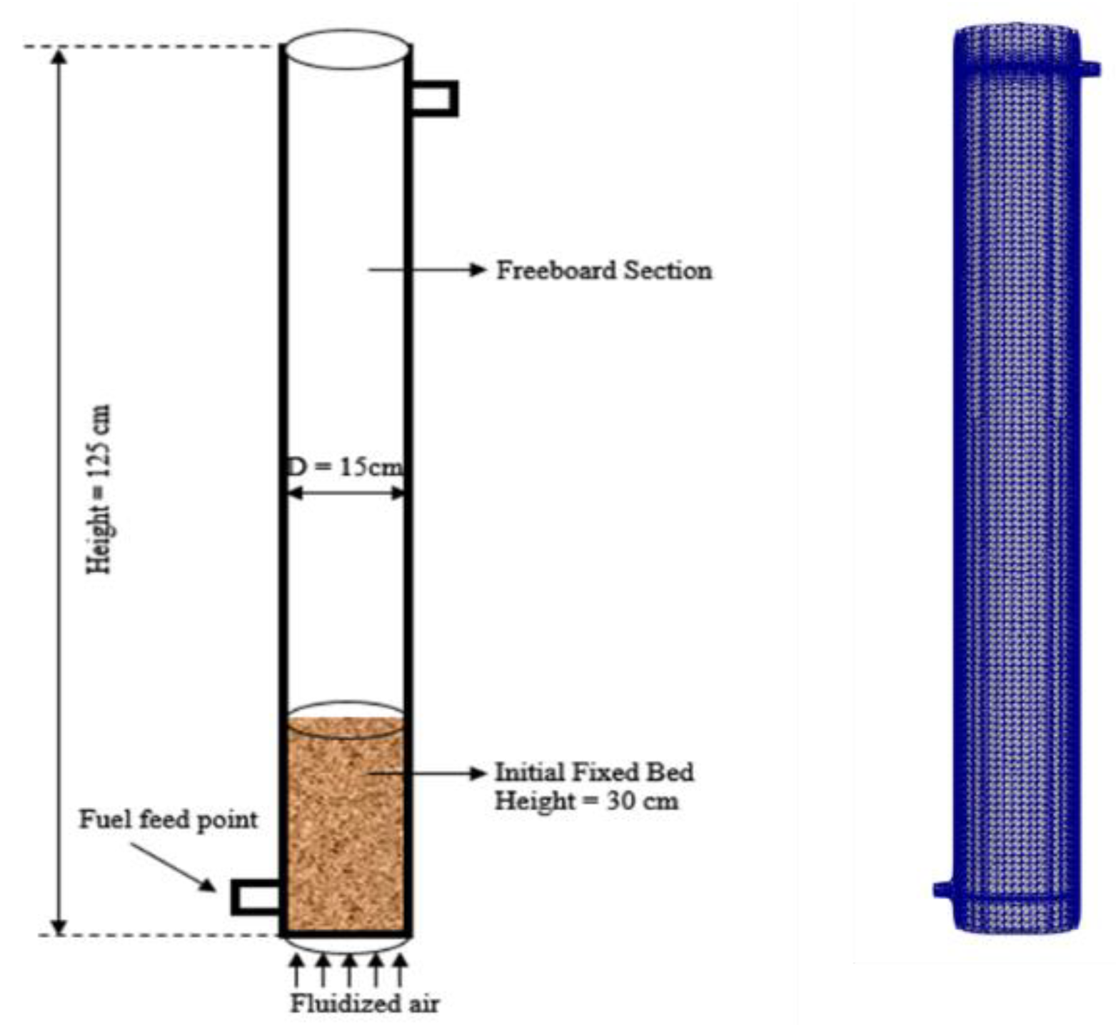
The fluidized gasifier selected for simulation is located at the University of Northern California and is shown (with a test stand) in Figure 1 [33]. The gasification reactor is 125 cm high with an inner diameter of 15 cm and an outer diameter of 20 cm. The outer wall of the reactor is wrapped with high-temperature-resistant insulation material and can be regarded as an adiabatic wall. The bed material in the fluidization reactor is quartz sand with a particle size of 200 μm and a density of 2648 kg/m³. In the initial state, it was deposited at the bottom of the reactor with a height of 30 cm and a porosity of 0.43. The reactor is in a pure nitrogen environment. The fluidized air temperature at the bottom of the reactor is 950 K, and fuel enters from the left inlet at the bottom of the reactor. After entering the reactor, the fuel is mixed with the bed material for the gasification reaction. The average particle size of biomass fuel particles is 600 μm, and the density is 1126.8 kg/m³. The industrial analysis and elemental analysis of the biomass fuel particles are shown in

Table 3. Industrial analysis and elemental analysis of biomass particles.

Components	Unit	Value
Moisture	%	10.1
Ash	%	6.4
Volatile	%	67.2
Fixed carbon	%	16.3
C	%	49.4
H	%	43.6
O	%	6.1
N	%	0.7
S	%	0.17

.

In simulations, the quality of the mesh has a huge impact on the calculation results. Too sparse of a grid will lead to an inaccurate reduction of the detailed flow field inside the gasifier, while too dense of a grid will significantly increase calculation cost. Meanwhile, if the grid size is smaller than the particle size, it will lead to the absence of solid-phase calculations in the simulation. As shown in Figure 1, Cartesian grids are used for simulation objects, and the grids are refined at the bottom dense phase area and near the exit so as to simulate the complex flow and reaction process inside the actual system as much as possible. The MFIX developed by NETL is used to calculate the gas–solid two-phase flow in the gasifier. On the basis of the flow calculation, chemical reaction models are added and recompiledto simulate the complex gas–solid flow reaction in the gasifier.

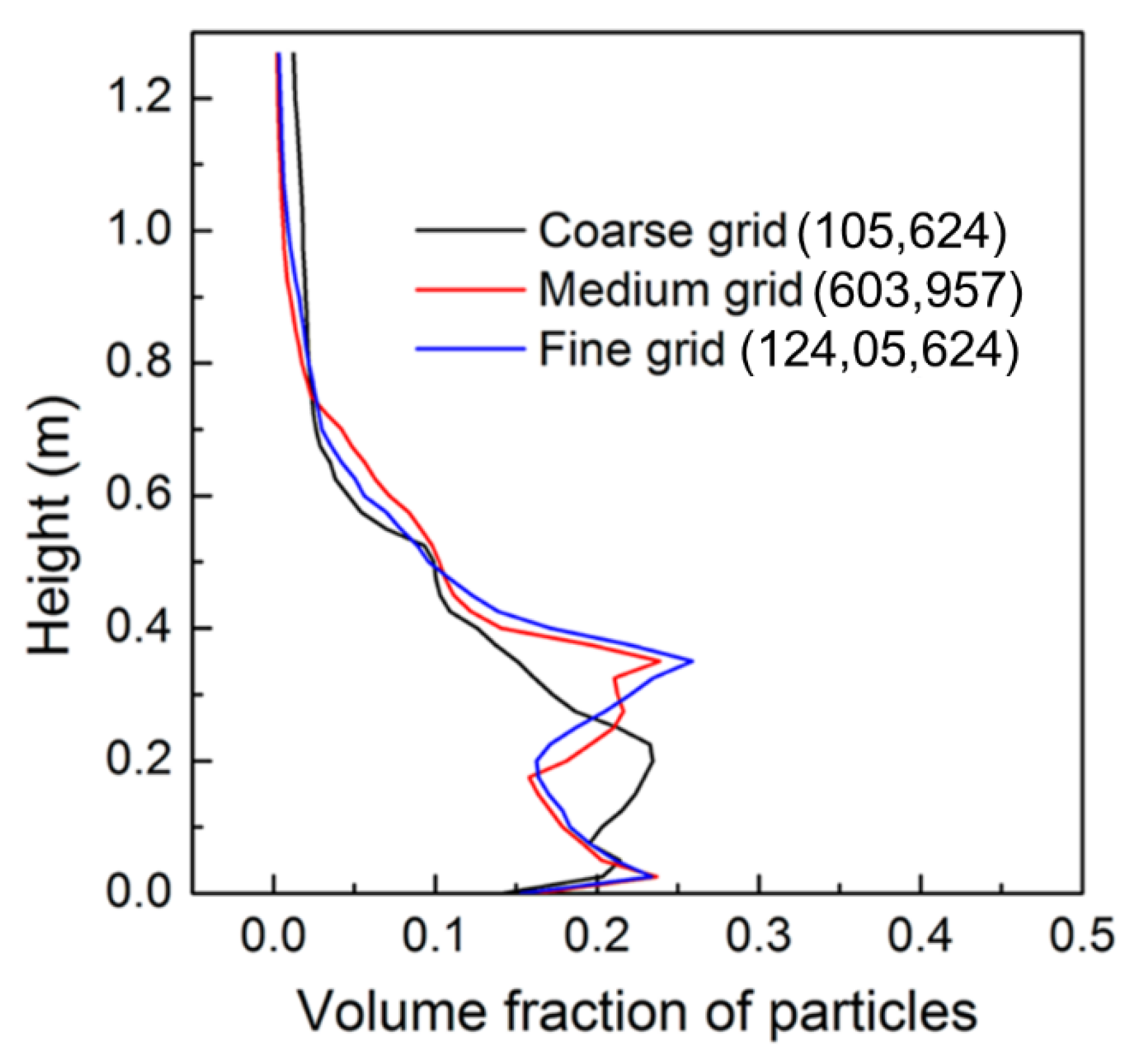
Grid resolution has a great influence on the calculation results. Three different grid resolutions are used for testing. It can be seen from Figure 2 that there is a big difference between the coarse grid and the two external grids in the bottom dense phase area, whereas the calculation results of the medium grid and the fine grid have little difference; the medium grid is chosen as the calculation grid. After grid independence verification, the grid number in this calculation is about 60 w.

4. Simulation Conditions

The generation of gasification products of biomass fuel is closely related to reaction temperature and equivalence ratio. The equivalence ratio is defined as the ratio of the actual fuel/air ratio to the stoichiometric fuel/air ratio.

$$ER=\frac{{\left({\dot{M}}_{O_2}/{\dot{M}}_{fuel}\right)}_{actual}}{{\left({\dot{M}}_{O_2}/{\dot{M}}_{fuel}\right)}_{stoic}}=\frac{{\left({\dot{\eta }}_{O_2}/{\dot{\eta }}_{fuel}\right)}_{actual}}{{\left({\dot{\eta }}_{O_2}/{\dot{\eta }}_{fuel}\right)}_{stoic}}$$

(15)

For gasification reactors, if the equivalent ratio is too large, part of the syngas will participate in the combustion reaction, which is not conducive to the generation of syngas at the final reactor outlet. Conversely, if the equivalent ratio is too small, the reaction heat source may not be enough to hold the temperature in the fluidized bed. Initial bed temperature also has a significant impact on syngas generation. Fuel and air are quickly mixed with the bed after entering the reactor and heated to the reaction temperature. After that, the whole system is in a self-sustaining and sustainable reaction state, so choosing the right initial bed temperature is also critical. To further study the factors influencing the syngas generation of the gasifier, different initial bed temperatures and equivalent ratio ER are selected in the simulation process.

In the simulation, the mass flowrate of biomass fuel entering the reactor is 68.04 kg/h, the fuel temperature is 298.15 K, and the inlet air temperature is 950 K. The initial static stacking height of the bed material is 30 cm. According to the different equivalence ratios, the inlet air mass flowrate is divided into three groups: 81 Nm³/h, 121.68 Nm³/h, and 162 Nm³/h. Initial bed temperature in gasification is divided into 1000 K, 1050 K, and 1100 K. The Euler–Euler model was selected to simulate gas–solid flow in the fluidized reactor during reaction. The main simulation conditions are shown in

Table 4. The main simulation conditions.

ER	Initial Bed Temperature (K)	Flowrate of Air (Nm3/h)
0.2	1000	81
0.2	1050	81
0.2	1100	81
0.3	1000	121.68
0.3	1050	121.68
0.3	1100	121.68
0.4	1000	162
0.4	1050	162
0.4	1100	162

below.

Table 5. Boundary conditions.

	Gas Phase	Solid Phase
Inlet	$u_g$	$u_{s,in}={\mathrm{G}}_s/\left({\alpha }_s{\rho }_s\right)$
	$k_{in}=0.004u_{g,in}^2$ ${\epsilon }_{in}=2k_{in}^{0.75}/(\kappa d)$$,\kappa =0.4187$
Wall	$u=v=0$$,k=0$$,\frac{\partial \epsilon }{\partial r}=0$	$u=0$$,k=0$$,\frac{\partial \epsilon }{\partial r}=0$$e_w=0.8$
Outlet	$\frac{\partial \phi }{\partial x}=0$$,\phi =u,v,k,\epsilon$

shows the boundary conditions used in simulation. In order to ensure the stability of numerical calculation, the Courant number should be less than 1 in the calculation process. At the same time, in order to ensure convergence and efficiency of calculation, the calculated time step is 5 × 10⁻⁴ s. The total simulation time is 20 s.

5. Results and Discussion

The distribution of the gas–solid flow field is very important for the reaction calculation in the gasification reaction system. The distribution of the gas–solid flow field and component field in the system closely affects the chemical reaction. Therefore, it is necessary to verify the reliability of the calculation of the internal flow field before studying the factors influencing gasifier gas production. Before calculation of these nine working conditions, the gas–solid flow field calculation results in the Euler–Euler model are firstly calculated and analyzed. On this basis, the reaction process is added to the simulation to analyze the change of gas components in the furnace and the main factors affecting the synthesis of gas generation.

5.1. Gas–Solid Flow in Fluidized Bed Gasifier

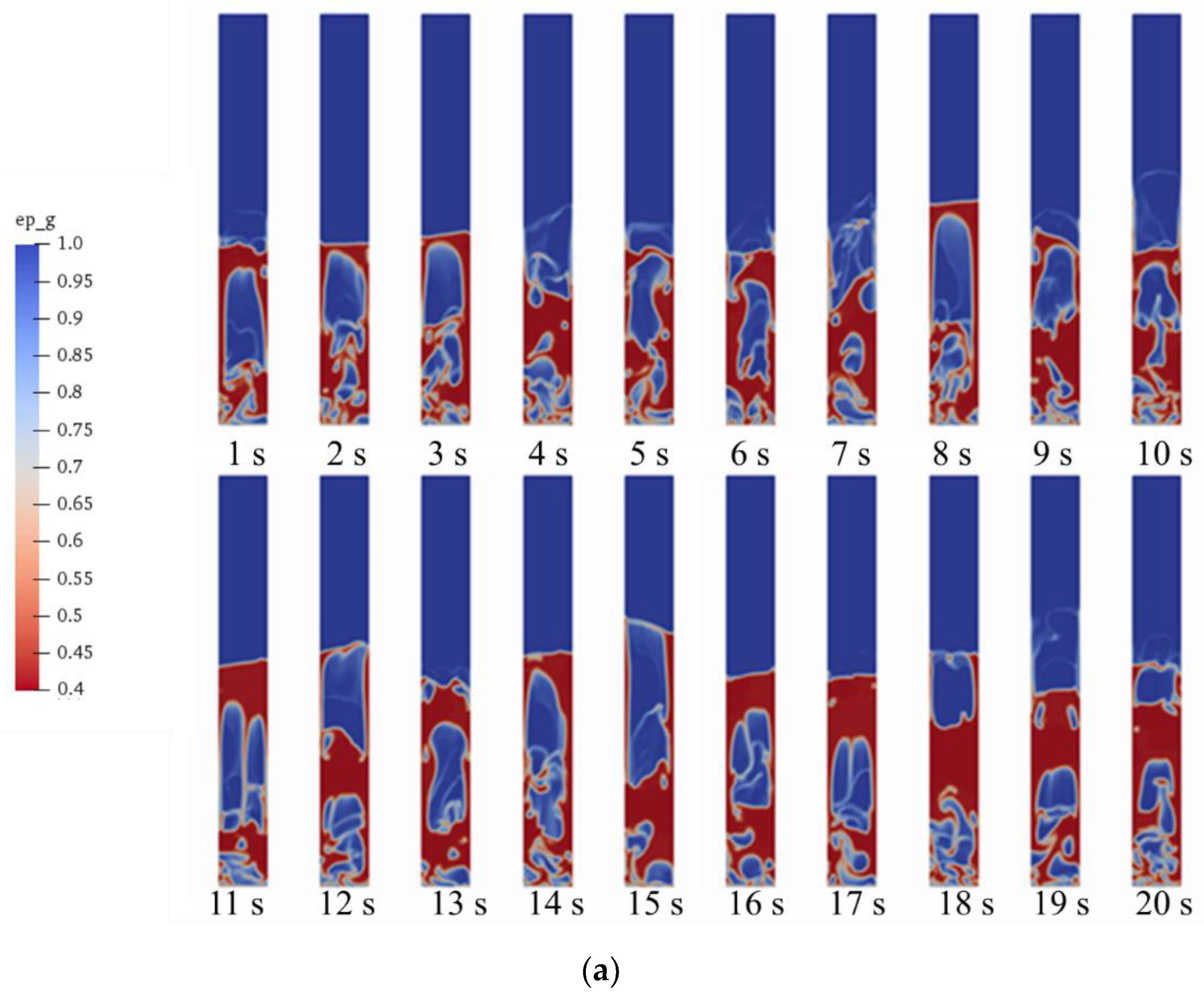
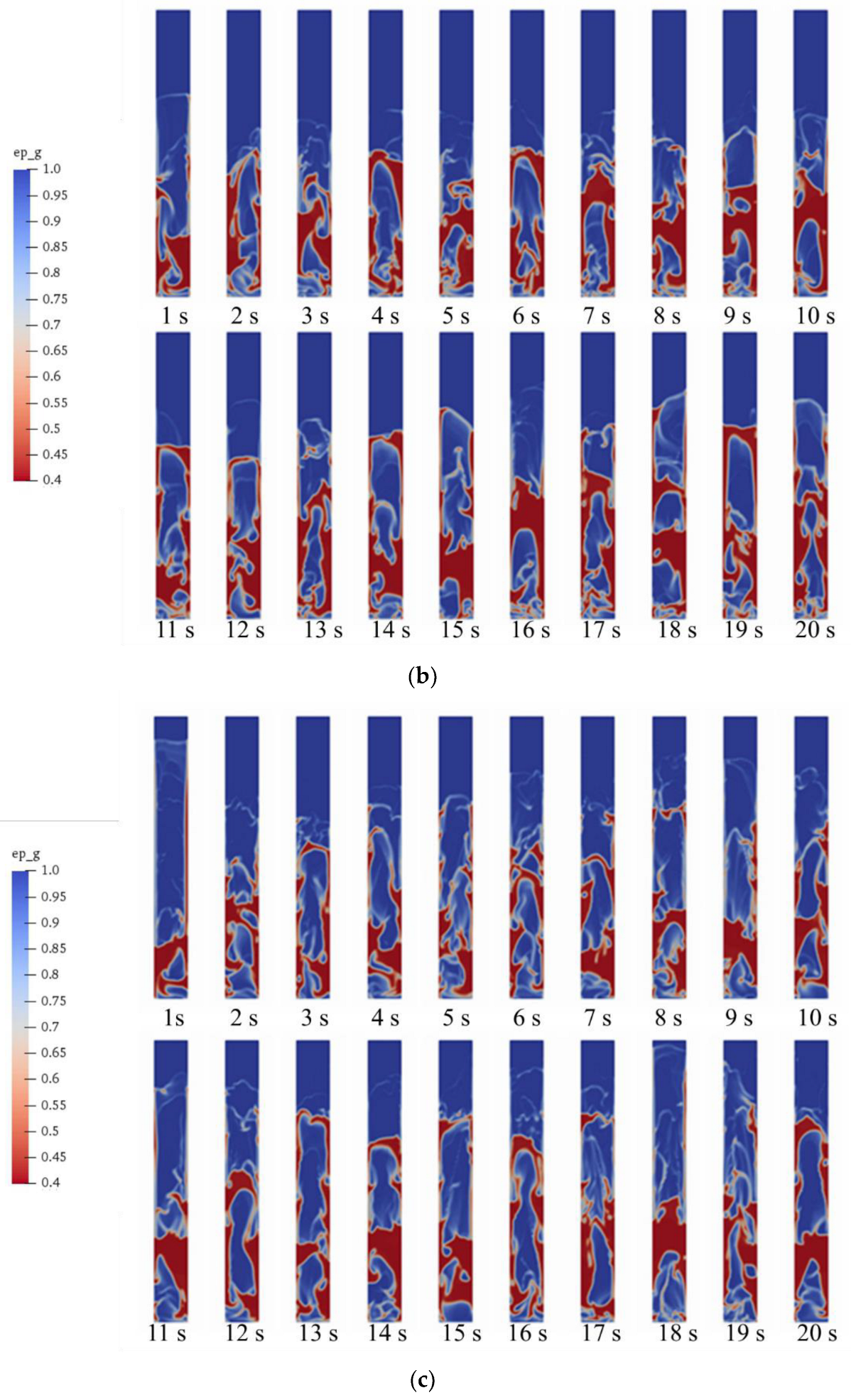
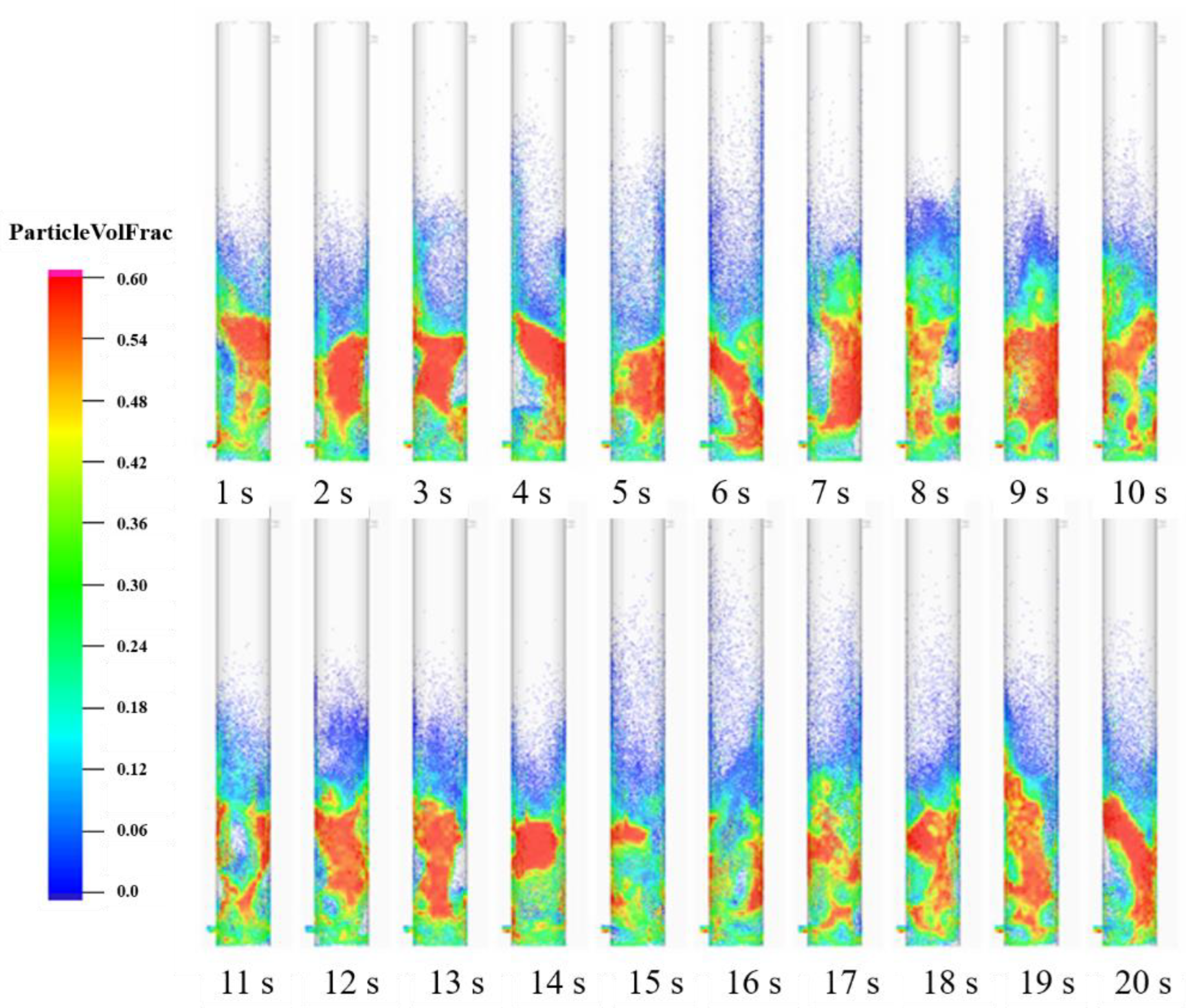
Before the coupling reaction, the initial bed temperature of 1050 K and equivalence ratios of 0.2, 0.3, and 0.4 are selected to simulate the gas–solid flow in the fluidized bed, and the reaction in the reactor is not considered in this process. Figure 3a–c show the changes in the gas–solid flow field simulated by the Euler–Euler model over time when the initial bed temperature is 1050 K and the equivalence ratio is 0.2, 0.3, and 0.4, respectively. Red represents the particle phase, darker color represents a larger volume share of the particle phase, and blue represents the gas phase. It can be seen from the three groups of pictures that bubbles are generated and broken in the bubbling gasification bed. With the increase in the equivalence ratio, the flow of air volume into the bottom of the reactor increases, and the average height of the bubbling bed also increases. After 4–5 s, the gasifier is basically in a stable bubbling fluidized state.

To verify the accuracy of gas–solid flow calculations, results are compared with previous studies using the Euler–Lagrange method. Figure 4 below is the calculation result obtained by using MP-PIC. The stable bed height calculated by the two methods is about 55 cm, and a similar cavitation structure is formed in the solid phase region. The formation and breaking of cavitation bubbles is similar. The size and shape of cavitation in the dense phase region is not much different, and the diameter of cavitation can reach 10–15 cm before crushing. At the same time, it can be seen from the two figures that the volume fraction of solid particles has certain similarity in the whole fluidized bed area. Through comparison, the accuracy of the two-fluid model based on KTGF was verified, and application of this subsequent chemical reaction model laid a baseline.

5.2. Chemical Reaction Model Validation

For the simulation of a fluidized bed gasifier accompanied by a homogeneous reaction of gas–solid two-phase flow, the heterogeneous reaction’s influence on the result is very big, so choosing the appropriate chemical reaction model is essential. The experimental data [34] are compared with the calculated results to verify the accuracy of the model. As can be seen from

Table 6. Compared Simulation Results with Experimental Results.

	Experiment	Simulation
Biomass feed rate (kg/h)	74.8	75
Air (Nm3/h)	84.5	81
ER	0.22	0.2
Gasification Temperature (°C)	815	800
Gas Composition (dry vol. %)
H2	14.7	17.71
CO2	11.8	5.94
O2	0.00	0.00
CO	20.2	20.1
CH4	4.4	3.77
N2	49.0	52.48

at the same gasification temperature and ER, the main components of biomass fuel gasification are the same, and the molar share of each major gas component is not much different, which proves that the model has a fairly high accuracy for the simulation of the gasification reaction.

5.3. Distribution of Syngas Components in the Gasifier

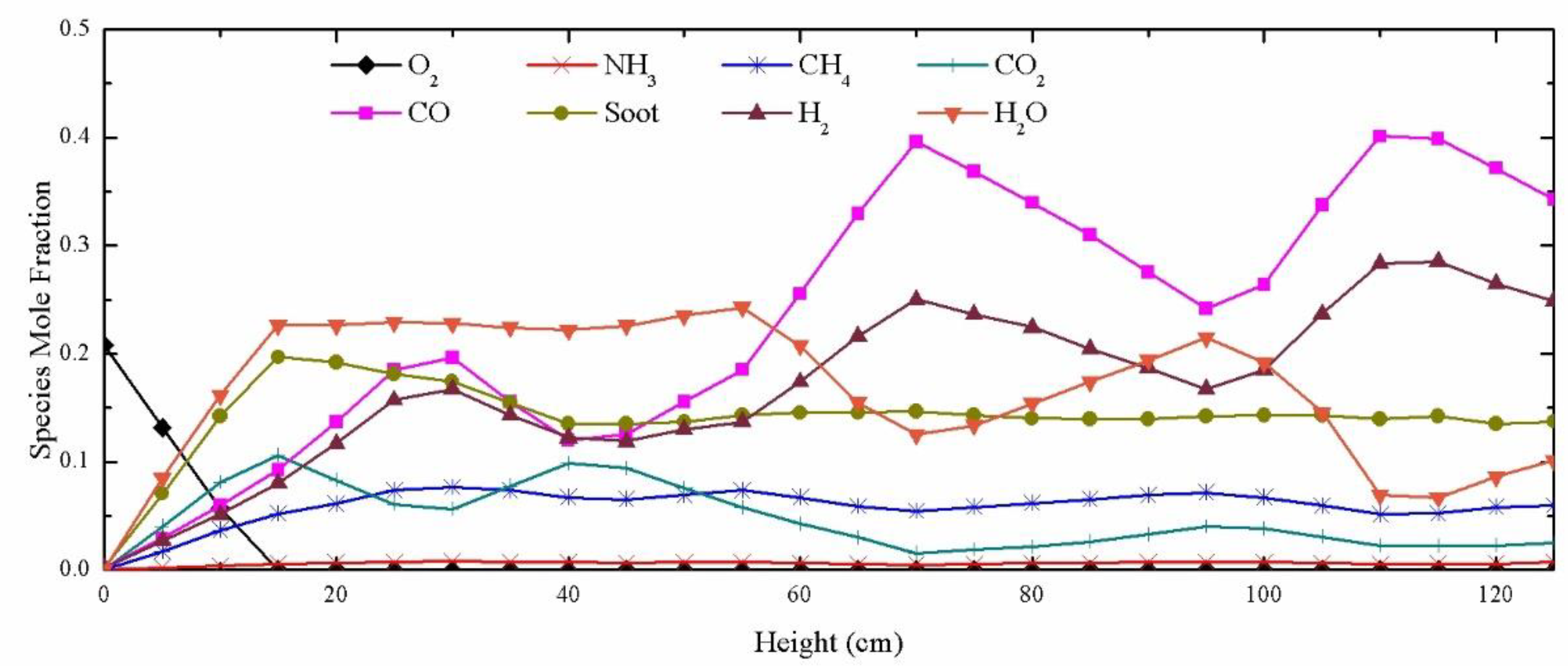
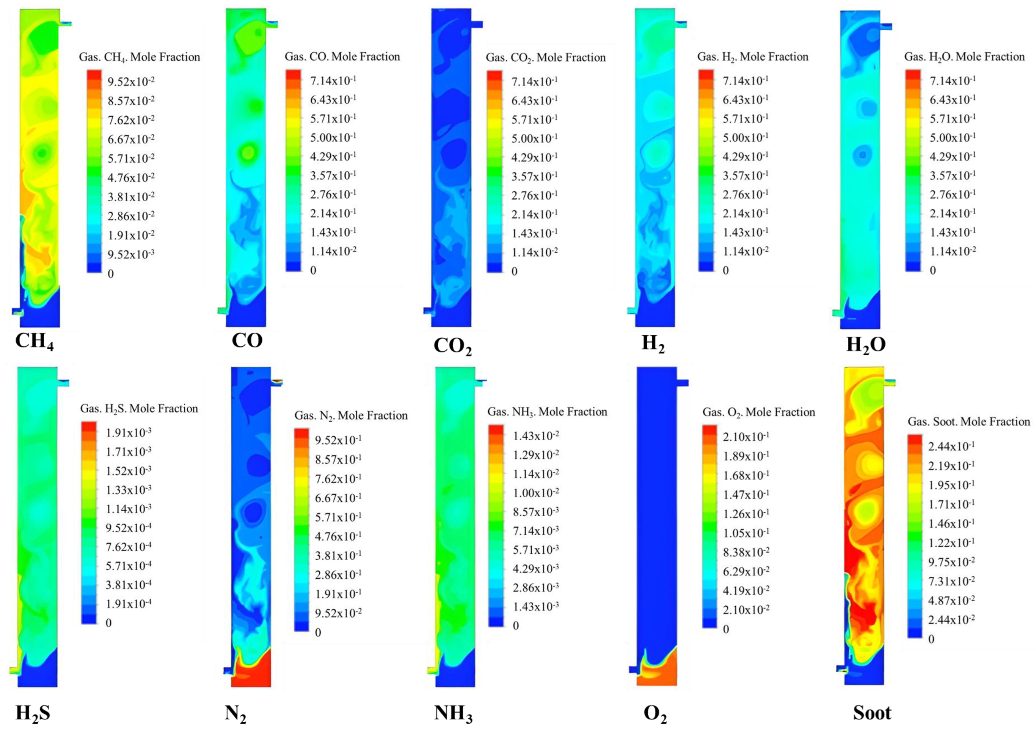
A coupling gas–solid flow reaction simulation is carried out for each working condition in Table 4. The results of 5–20 s after gas–solid flow stabilization in the gasifier were averaged to obtain the distribution of gases of each component in the furnace reactor. Figure 5 shows the distribution of each gas component along with the height of the reactor under the first group of working conditions, and Figure 6 shows the distribution of each gas component in the middle section of the reactor.

When oxygen enters the reactor, it reacts with combustible gas or coke to release heat, and its concentration decreases as height increases. Since the equivalence ratio entering the reactor is generally less than 1 in the gasification reaction, oxygen is gradually consumed in the reactor until it is negligible in the upper region.

As one of the main components of the syngas produced by the gasifier, the concentration of carbon monoxide increases briefly at first, then decreases slightly and increases again. This suggests that the rate of carbon monoxide generation at different heights varies: in the bottom of the reactor, the rise of carbon monoxide concentration is mainly due to volatile thermolysis and water–gas reaction; with increasing height, volatile matter and water vapor is consumed, dominating the combustion process and decreasing the carbon monoxide concentration; after the oxygen in the reactor has been used up, carbon monoxide is produced by reduction of carbon dioxide, which increases concentration with increasing height.

As another major component of syngas, the concentration of hydrogen does not vary as much as that of carbon monoxide, and its molar concentration increases with height. Hydrogen concentration increases continuously because of the water–gas displacement reaction. Oxygen is mainly consumed by other gas components—the hydrogen oxidation reaction is relatively slow.

5.4. Analysis of Factors Influencing Syngas Generation

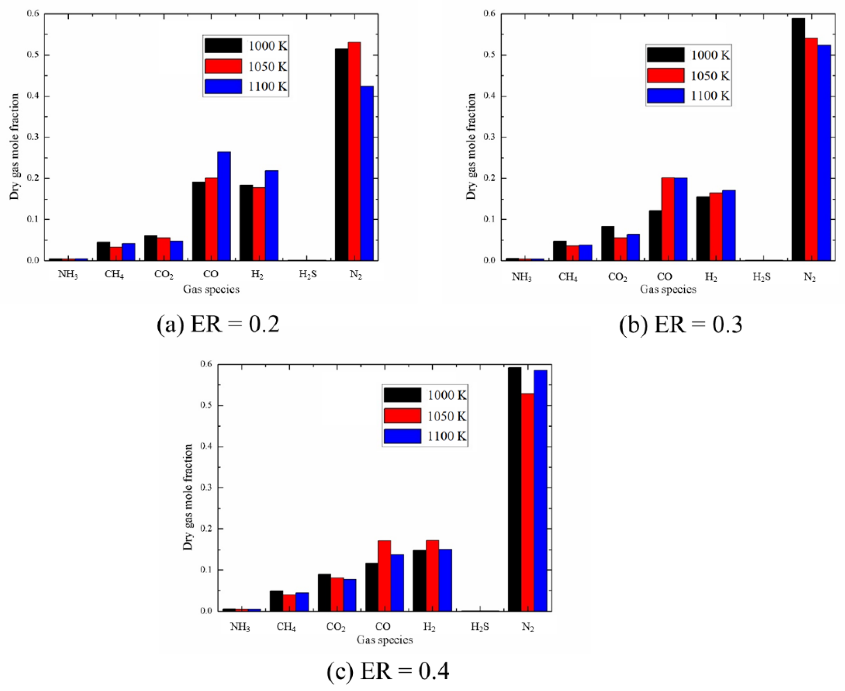
Figure 7a–c shows the influence of initial bed temperature (1000 K, 1050 K, and 1100 K) on gasification products at different equivalence ratios (ER = 0.2, 0.3, and 0.4). The ordinate is the average molar concentration of each gas component at the reactor outlet from 5–15 s. Because higher temperature is more conducive to gas–solid phase heterogeneous reactions [29,30], especially water evaporation and water–gas replacement reactions, the molar concentrations of CO and H₂ at the outlet of the reactor increase with increased initial bed temperature. With the increase in temperature, the CO₂ reduction reaction rate accelerates, which decreases CO₂ concentration at the outlet. Higher temperatures are more favorable for gasification reactors, resulting in higher concentrations of CO and H₂ in syngas at the outlet.

The equivalence ratio for syngas depends mainly on the effects of O₂. The equivalence ratio increases with increased O₂ volume in the inlet air. This can lead to oxidation and combustion of part of the synthesized CO and H₂ in the reactor.

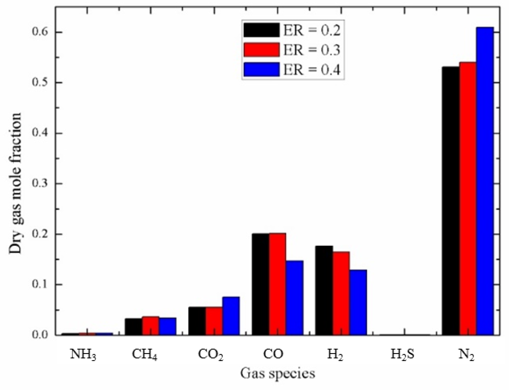
Figure 8 shows the effect of different equivalence ratios (0.2, 0.3, and 0.4) on gasification products at an initial bed temperature of 1050 K. As can be seen from the Figure, with the increase in equivalence ratio, the concentration of CO₂ at the outlet keeps increasing, which is mainly due to the increase of oxygen in the reactor, which accelerates the coke combustion reaction. As the equivalence ratio increases, the concentration of H₂ and CO in the syngas decreases, which is also due to the increased O₂ concentration. When the initial bed temperature is 1050 K and the equivalence ratio increases from 0.2 to 0.4, the molar concentration of CO in syngas decreases from about 20% to 15.1%, H₂ decreases from 16.82% to 11.43%, and CO₂ increases from 6.48% to 8.22%.

6. Conclusions

In this paper, a three-dimensional Euler–Euler two-fluid model of a bubbled fluidized gasifier is established. Based on the calculation results, the factors influencing syngas generation in a gasifier were analyzed. According to the different equivalence ratios and initial bed temperatures, the simulation was divided into nine working conditions. It was found that the initial bed temperature has a great influence on the generation of syngas. With the increase of temperature, the molar concentration of CO and H₂ in syngas increases. Although the gasification reaction in gasifier reactors is a self-sustaining and sustainable reaction under certain conditions, the initial bed temperature can significantly affect volatilization and pyrolysis of the fuel after entering the reactor, resulting in a new balance between endothermic and exothermic reactions. The research on equivalence ratios shows that with the increase of equivalence ratio, the oxygen entering the furnace increases, and the syngas generated in the gasification process is oxidized and consumed in the oxygenated environment, decreasing syngas output. Although the research object in this paper was a laboratory-scale fluidized bed gasifier, the Euler–Euler two-fluid model proved to be an effective analytical method for simulating a fluidized bed gasifier. The model in this paper can be extended to a larger industrial scale to provide strong support for efficient and clean utilization of biomass energy.

References

- Odgaard, O.; Delman, J. China’s energy security and its challenges towards 2035. Energy Policy 2014, 71, 107–117. [Google Scholar] [CrossRef]
- Guo, X.; Xiao, B.; Zhang, X.; Luo, S.; He, M. Experimental study on air-stream gasification of biomass micron fuel (BMF) in a cyclone gasifier. Bioresour. Technol. 2009, 100, 1003–1006. [Google Scholar] [CrossRef] [PubMed]
- Ngusale, G.K.; Luo, Y.; Zhang, R.-z.; Yin, R.-h.; Zhao, W.-l. Gasification of wood pellets in a bench-scale updraft gasifier. Energy Sources Part A Recovery Util. Environ. Eff. 2016, 38, 1875–1881. [Google Scholar] [CrossRef]
- Wu, K.; Ren, T.; Chen, H.; Zhu, Y. Experimental investigation of whole tires and biomass mixed firing in reverse burning fixed-bed gasifier. Energy Procedia 2017, 105, 583–589. [Google Scholar] [CrossRef]
- You, Z.; You, S.; Ma, X. Studies on Biomass Char Gasification and Dynamics; IOP Conference Series: Earth and Environmental Science; IOP Publishing: Bristol, UK, 2018; p. 052032. [Google Scholar]
- Zhang, Z.; Pang, S. Experimental investigation of biomass devolatilization in steam gasification in a dual fluidised bed gasifier. Fuel 2017, 188, 628–635. [Google Scholar] [CrossRef]
- Ding, J.; Gidaspow, D. A bubbling fluidization model using kinetic theory of granular flow. AIChE J. 1990, 36, 523–538. [Google Scholar] [CrossRef]
- Lathouwers, D.; Bellan, J. Modeling of dense gas–solid reactive mixtures applied to biomass pyrolysis in a fluidized bed. Int. J. Multiph. Flow 2001, 27, 2155–2187. [Google Scholar] [CrossRef]
- Lathouwers, D.; Bellan, J. Yield optimization and scaling of fluidized beds for tar production from biomass. Energy Fuels 2001, 15, 1247–1262. [Google Scholar] [CrossRef]
- Zhang, H.; Yu, C.; Luo, Z.; Li, Y.A. Investigation of Ash Deposition Dynamic Process in an Industrial Biomass CFB Boiler Burning High-Alkali and Low-Chlorine Fuel. Energies 2020, 13, 1092. [Google Scholar] [CrossRef] [Green Version]
- Yu, X.; Blanco, P.H.; Makkawi, Y.; Bridgwater, A.V. CFD and experimental studies on a circulating fluidised bed reactor for biomass gasification. Chem. Eng. Process.-Process Intensif. 2018, 130, 284–295. [Google Scholar] [CrossRef] [Green Version]
- Xu, Y.; Liu, X.; Qi, J.; Zhang, T.; Xu, M.; Fei, F.; Li, D. Compositional and structural study of ash deposits spatially distributed in superheaters of a large biomass-fired CFB boiler. Front. Energy 2021, 15, 449–459. [Google Scholar] [CrossRef]
- Unchaisri, T.; Fukuda, S.; Phongphipat, A.; Saetia, S.; Sajjakulnukit, B. Experimental study on combustion characteristics in a CFB during Co-firing of coal with biomass pellets in Thailand. Int. Energy J. 2019, 19, 101–114. [Google Scholar]
- Ahmad, A.A.; Zawawi, N.A.; Kasim, F.H.; Inayat, A.; Khasri, A. Assessing the gasification performance of biomass: A review on biomass gasification process conditions, optimization and economic evaluation. Renew. Sustain. Energy Rev. 2016, 53, 1333–1347. [Google Scholar] [CrossRef]
- Tang, Y.-l.; Liu, D.-j.; Liu, Y.-h.; Luo, Q. 3D computational fluid dynamics simulation of natural coke steam gasification in general and improved fluidized beds. Energy Fuels 2010, 24, 5602–5610. [Google Scholar] [CrossRef]
- Loha, C.; Gu, S.; De Wilde, J.; Mahanta, P.; Chatterjee, P.K. Advances in mathematical modeling of fluidized bed gasification. Renew. Sustain. Energy Rev. 2014, 40, 688–715. [Google Scholar] [CrossRef]
- Wu, H.; Yang, C.; He, H.; Huang, S.; Chen, H. A hybrid simulation of a 600 MW supercritical circulating fluidized bed boiler system. Appl. Therm. Eng. 2018, 143, 977–987. [Google Scholar] [CrossRef]
- Yang, C.; Wu, H.; Deng, K.; He, H.; Sun, L. Study on Powder Coke Combustion and Pollution Emission Characteristics of Fluidized Bed Boilers. Energies 2019, 12, 1424. [Google Scholar] [CrossRef] [Green Version]
- Ismail, T.M.; Ramos, A.; Monteiro, E.; Abd El-Salam, M.; Rouboa, A. Parametric studies in the gasification agent and fluidization velocity during oxygen-enriched gasification of biomass in a pilot-scale fluidized bed: Experimental and numerical assessment. Renew. Energy 2020, 147, 2429–2439. [Google Scholar] [CrossRef]
- Chapman, S.; Cowling, T.G. The Mathematical Theory of Non-Uniform Gases: An Account of the Kinetic Theory of Viscosity, Thermal Conduction and Diffusion in Gases; Cambridge University Press: Cambridge, UK, 1990. [Google Scholar]
- Jenkins, J.T.; Savage, S.B. A theory for the rapid flow of identical, smooth, nearly elastic, spherical particles. J. Fluid Mech. 1983, 130, 187–202. [Google Scholar] [CrossRef]
- Syamlal, M.; O’Brien, T.J. Computer simulation of bubbles in a fluidized bed. AIChE Symp. Ser. 1989, 85, 22–31. [Google Scholar]
- Snider, D.M.; Clark, S.M.; O’Rourke, P.J. Eulerian–Lagrangian method for three-dimensional thermal reacting flow with application to coal gasifiers. Chem. Eng. Sci. 2011, 66, 1285–1295. [Google Scholar] [CrossRef]
- Srinivas, S.; Field, R.P.; Herzog, H.J. Modeling tar handling options in biomass gasification. Energy Fuel 2013, 27, 2859–2873. [Google Scholar] [CrossRef]
- Li, C.; Suzuki, K. Tar property, analysis, reforming mechanism and model for biomass gasification—An overview. Renew. Sustain. Energy Rev. 2009, 13, 594–604. [Google Scholar] [CrossRef]
- Syamlal, M.; Bissett, L.A. METC Gasifier Advanced Simulation (MGAS) Model; USDOE Morgantown Energy Technology Center: Morgantown, WV, USA, 1992.
- Hobbs, M.L.; Radulovic, P.T.; Smoot, L.D. Modeling fixed-bed coal gasifiers. Aiche J. 1992, 38, 681–702. [Google Scholar] [CrossRef]
- Armstrong, L.-M.; Gu, S.; Luo, K.H. Effects of limestone calcination on the gasification processes in a BFB coal gasifier. Chem. Eng. J. 2011, 168, 848–860. [Google Scholar] [CrossRef] [Green Version]
- Armstrong, L.; Gu, S.; Luo, K. Parametric study of gasification processes in a BFB coal gasifier. Ind. Eng. Chem. Res. 2011, 50, 5959–5974. [Google Scholar] [CrossRef]
- He, P.-w.; Luo, S.-y.; Cheng, G.; Xiao, B.; Cai, L.; Wang, J.-b. Gasification of biomass char with air-steam in a cyclone furnace. Renewable Energy 2012, 37, 398–402. [Google Scholar] [CrossRef]
- Gerber, S.; Behrendt, F.; Oevermann, M. An Eulerian modeling approach of wood gasification in a bubbling fluidized bed reactor using char as bed material. Fuel 2010, 89, 2903–2917. [Google Scholar] [CrossRef]
- Xiao, R.; Zhang, M.; Jin, B.; Huang, Y.; Zhou, H. High-temperature air/steam-blown gasification of coal in a pressurized spout-fluid bed. Energy Fuels 2006, 20, 715–720. [Google Scholar] [CrossRef]
- Liu, H.; Elkamel, A.; Lohi, A.; Biglari, M. Computational fluid dynamics modeling of biomass gasification in circulating fluidized-bed reactor using the Eulerian–Eulerian approach. Ind. Eng. Chem. Res. 2013, 52, 18162–18174. [Google Scholar] [CrossRef]
- Radmanesh, R.; Chaouki, J.; Guy, C. Biomass gasification in a bubbling fluidized bed reactor: Experiments and modeling. AIChE J. 2006, 52, 4258–4272. [Google Scholar] [CrossRef]
Figure 1.
Schematic of fluidized bed gasifier.
Figure 2.
Profiles of solid concentrations with different grid sizes.
Figure 3.
(a) Gas–solid flow field in gasifier (ER 0.2); (b) gas–solid flow field in gasifier (ER 0.3); (c) gas–solid flow field in gasifier (ER 0.4).
Figure 4.
The gas–solid flow field in gasifier based on MP-PIC (ER 0.2).
Figure 5.
Distribution of molarity concentration of each component along with height (ER = 0.2; T = 1000 K).
Figure 6.
Mole fraction distributions of different gases in the middle section of the gasifier (ER = 0.2; T = 1000 K).
Figure 7.
Molar concentrations of syngas components at different initial bed temperatures (ER = 0.2).
Figure 8.
Molar concentrations of syngas components at different ERs (1050 K).