
Energy Consumption Estimation for Electric Buses Based on a Physical and Data-Driven Fusion Model


1
College of Physics and Optoelectronic Engineering, Shenzhen University, Shenzhen 518060, China
2
National Engineering Laboratory for Electric Vehicles, School of Mechanical Engineering, Beijing Institute of Technology, Beijing 100081, China
3
Guangdong Laboratory of Artificial Intelligence and Digital Economy (SZ), Shenzhen University, Shenzhen 518060, China
*
Author to whom correspondence should be addressed.
Energies 2022, 15(11), 4160; https://doi.org/10.3390/en15114160
Submission received: 18 March 2022
/
Revised: 23 May 2022
/
Accepted: 2 June 2022
/
Published: 6 June 2022
(This article belongs to the Topic Energy Storage and Conversion Systems)
Abstract
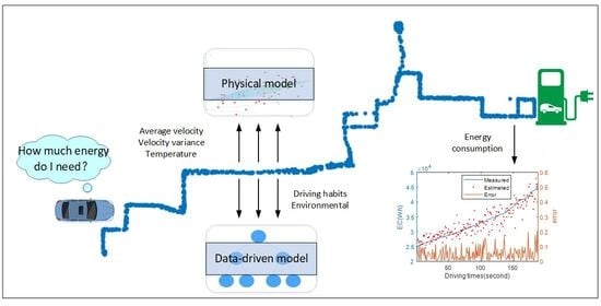
:The energy consumption of electric vehicles is closely related to the problems of charging station planning and vehicle route optimization. However, due to various factors, such as vehicle performance, driving habits and environmental conditions, it is difficult to estimate vehicle energy consumption accurately. In this work, a physical and data-driven fusion model was designed for electric bus energy consumption estimation. The basic energy consumption of the electric bus was modeled by a simplified physical model. The effects of rolling drag, brake consumption and air-conditioning consumption are considered in the model. Taking into account the fluctuation in energy consumption caused by multiple factors, a CatBoost decision tree model was constructed. Finally, a fusion model was built. Based on the analysis of electric bus data on the big data platform, the performance of the energy consumption model was verified. The results show that the model has high accuracy with an average relative error of 6.1%. The fusion model provides a powerful tool for the optimization of the energy consumption of electric buses, vehicle scheduling and the rational layout of charging facilities.
1. Introduction
With energy shortages and environmental pollution problems becoming more pronounced, the global energy structure is gradually undergoing a transformation. Countries around the world are taking steps to achieve sustainable, green and efficient energy systems. New energy vehicles, especially electric vehicles, are gaining widespread attention due to their low pollution and high energy efficiency. By the end of 2021, the number of new energy vehicles worldwide had exceeded 10 million. In the Chinese urban bus system, many diesel buses have been replaced by energy-efficient and environmentally friendly electric buses [1]. Compared to traditional diesel buses, electric buses have more advantages in the public transport system. However, there are still some problems, such as difficulties in charging demand evaluation, vehicle route planning and battery energy storage system design. These issues are closely related to the range of electric buses and the energy consumption of vehicles under specific operating conditions [2]. Therefore, the study of an accurate vehicle energy consumption estimation model can solve the above problems, which is of great significance to the popularization of electric buses. The driving energy consumption of electric buses is affected by drivers’ habits and working conditions. For electric buses on the same route, the difference in driving energy consumption under different working conditions can reach 40%. Therefore, information such as the temperature and departure time under current operating conditions need to be considered so as to accurately estimate the energy consumption of the vehicle.
The energy consumption of an electric vehicle is related to the vehicle powertrain dynamic performance, such as the windproof area of the vehicle, vehicle charging efficiency, etc. It is also influenced by the habits of drivers and environmental factors. As a result, it is difficult to achieve an accurate estimation of the energy consumption of a vehicle [3]. However, the national monitoring and management platform for new energy vehicles (NEVS) in China has enabled the aggregation of massive amounts of data on new energy vehicles. The platform can provide a large amount of vehicle driving data for the analysis and modeling of vehicle energy consumption.
Many related studies have been performed in this area. Yuan et al. [4] modeled vehicle powertrain dynamics by simulating driving data on a computer. An energy consumption model for electric vehicles was achieved. In the model, the energy of an electric vehicle is mainly consumed by rolling drag, air resistance and kinetic energy, and the error of the model is about 3%. However, the model only considers energy consumption under laboratory conditions and does not further consider possible congestion and air-conditioning factors in the actual driving process. Bracco et al. [5] used a simulation model to analyze the effects of different variables on energy consumption and the battery charging state. The results show that the number of passengers has the greatest impact on the energy consumption of electric vehicles. Qi et al. [6] used positive kinetic energy and negative kinetic energy to decompose the energy consumption under actual traffic congestion. Based on this decomposition, a data-driven model was established. The model is used to estimate the energy consumption of electric vehicles on the road, and the actual traffic conditions are taken into account. The model needs a lot of data input to obtain the accurate positive and negative kinetic energy of the vehicle. After simplifying the input to the average speed, the model error is 7%. Hao et al. [7] analyzed the energy consumption of electric buses, minibuses and taxis in Beijing. Through statistical analysis, vehicle energy consumption in different seasons and driving conditions was obtained. It was found that the energy consumption of electric vehicles per kilometer is lower than that at 5 °C. This shows that the energy transmission efficiency of the battery will change at different temperatures. Miraftabzadeh et al. [8] considered the driving route and weather conditions in the modeling process. Using a data-driven modeling method, the energy consumption prediction model of an electric taxi was established. In addition, by calculating the energy consumption of taxis on weekdays and weekends, the author compiled a taxi energy consumption table. The table shows that the month with the highest energy consumption of taxis in New York City is April, while July is the month with the lowest energy consumption. Al-Wreikat et al. [9] analyzed the effect of ambient temperature on the energy consumption of electric vehicles. They found that vehicles consumed 28% more energy at low temperatures of 0–15 degrees than at medium temperatures of 15–25 degrees. Björnsson et al. [10] designed a physical model of powertrain dynamics. The energy recovery performance in the braking process was analyzed. The research shows that under urban conditions, the energy regeneration potential per kilometer is higher under the condition of low average speed and multiple starts and stops. It lays a foundation for the study of the urban bus recovery coefficient. The energy consumption of electric vehicles has been modeled by many approaches.
According to the literature review, previous studies have considered physical modeling methods or artificial intelligence algorithms to obtain vehicle energy consumption models. However, vehicle energy consumption is the result of multiple factors. The energy consumption estimation results obtained by a single method or a single type of model are less reliable. Moreover, in practical applications, there is a lack of an energy consumption estimation model with limited input features for driving decision making. It is necessary to design a more reliable energy consumption estimation model with few input features. To address these issues, a physical and data-driven fusion model for vehicle energy consumption is proposed in this paper. Part of the energy consumed by the vehicle during driving can be expressed by physical formulas, such as the energy consumed by rolling resistance and air resistance [11]. The direct application of formula modeling will reduce the complexity of the model. Other driving factors also affect the driving energy consumption of vehicles, such as the vehicle departure time, the ambient temperature, etc. For these factors that cannot be expressed by the formula, the data-driven model is selected. Finally, the two models are fused to estimate vehicle energy consumption.
The content of each section is as follows: In Section 2, the statistical analysis of electric bus data is performed. The original data are preprocessed and reconstructed to obtain continuous data in the vehicle charging and driving cycle process. In Section 3, the energy consumption estimation model is designed. A physical vehicle energy consumption model is developed based on the powertrain dynamic performance of the electric bus. Model parameters are initially calibrated using the least-squares method. In addition, the factors affecting fluctuations in vehicle energy consumption, such as driving habits and environmental factors, are summarized and analyzed. The CatBoost decision tree model is used to characterize the effects. Finally, the two models are fused to obtain the final estimation result of vehicle energy consumption. In Section 4, the energy consumption estimation model is analyzed and validated. Some conclusions are presented in Section 5.
2. Data Statistics and Analysis
The electric bus data came from the National Monitoring and Management Platform for NEVS. The original data were collected by on-board terminals on electric buses and uploaded to the data platform. The dataset includes 38 items, such as the sampling time, battery management system (BMS) number, battery pack voltage, battery current, state of charge (SOC), minimum cell voltage, maximum cell voltage, minimum temperature, maximum temperature, etc. A detailed description of the items used in this paper is shown in Table 1. The data cover ten electric buses on the same bus route in one year. The travel distance is approximately 34 km. There are 24 stops along the route. After one round trip, the buses will be charged at the starting point of the bus stations. The purpose of this section is to process the original data and obtain the data on vehicle speed, data acquisition time, temperature, accelerator pedal value and deceleration pedal value. The data will be further processed for vehicle energy consumption modeling.
Data Processing and Analysis
The quality of the original electric bus data on the platform was not flawless. The acquired data often appeared to have outliers and missing values due to the influence of electromagnetic radiation and the unreliability of the circuit system. As a result, preprocessing of the original data was needed. During the process, data interpolation, outlier removal and data segmentation were performed.
The two main types of missing data are missing multiple rows and missing single features. For the first case, the data exhibit a discontinuity in specific intervals. Missing data were interpolated using the mean value [12]. For the latter case, the Lagrangian interpolation method was used to interpolate the data. Considering the outliers, the first quartile and the third quartile of the data were calculated by constructing a box plot. Values exceeding the upper and lower edges of the box plot were defined as outliers.
To facilitate the extraction of data features, the data were divided into short segments according to the state of charge in the dataset. The electric bus data transmission process and data preprocessing results are shown in Figure 1.
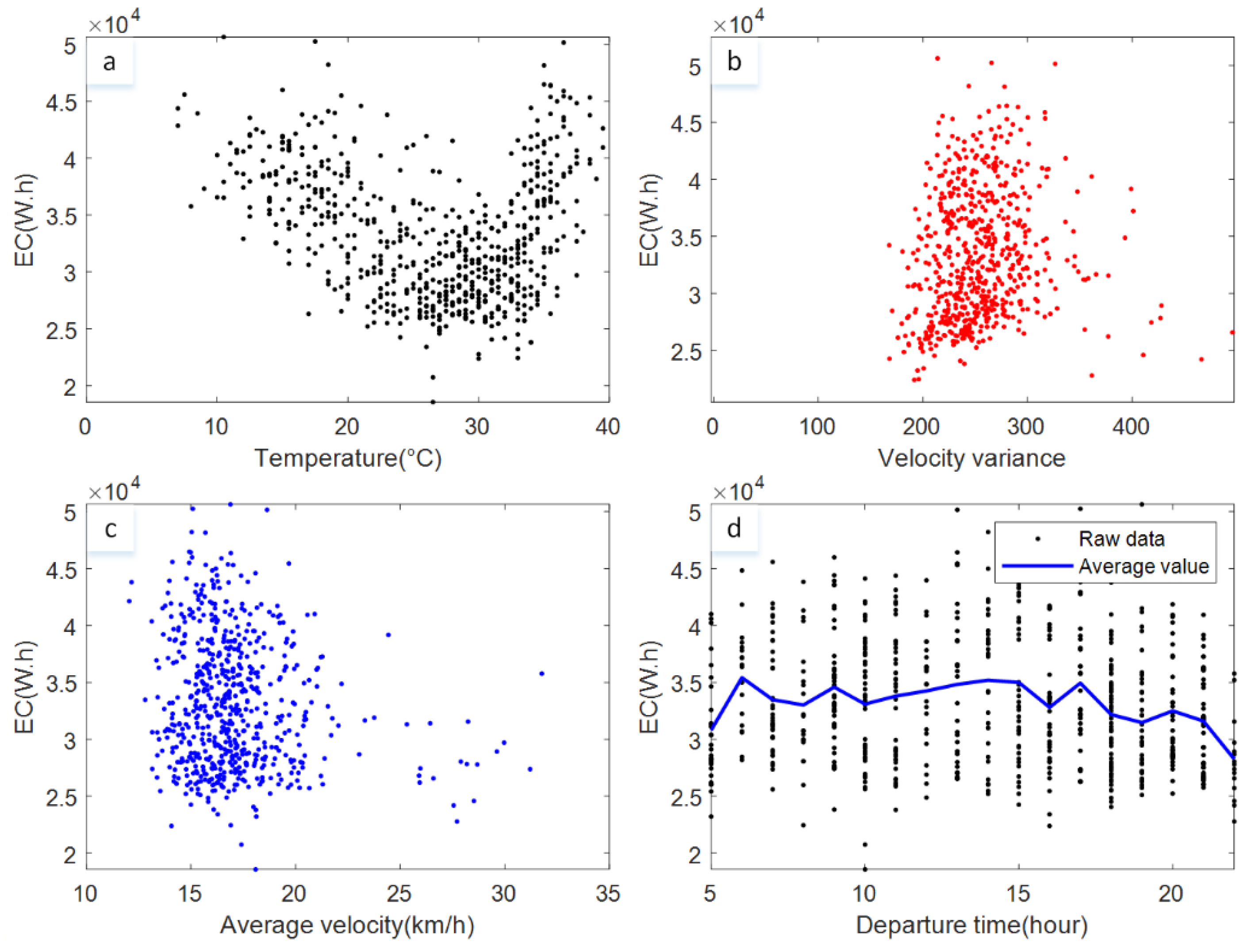
After preprocessing the original data, the data were reconstructed according to the timestamp, vehicle velocity, etc. The vehicle driving season, departure time and velocity-related features were obtained. The statistics of the vehicle energy consumption under different operating conditions are shown in Figure 2. In the figure, the heading of the ordinate is the energy consumption. For brevity, it is abbreviated as EC. For electric vehicles, the operating temperature is related to the use of air conditioning, energy efficiency, etc. Figure 2a shows the relationship between energy consumption and operating temperature. It can be seen that the relationship can be approximated by a parabolic function. The minimum energy consumption occurs at a temperature of approximately 25 degrees. This phenomenon coincides with the fact that air conditioning and high energy transfer efficiency are rarely used [6]. Figure 2b shows the relationship between the variance of velocity and energy consumption. It can be seen that there is an approximately linear relationship between them. The higher the variance, the higher the energy consumption. As shown in Figure 2c, there is no obvious linear relationship between average speed and energy consumption, and this part of the analysis is described in detail later. Figure 2d shows the relationship between departure time and energy consumption. Departure times are related to road congestion and vehicle passenger weight. Specifically, vehicles consume more energy between 6 a.m. and 8 p.m. Vehicle energy consumption values differ by more than 20%.
3. Vehicle Energy Consumption Modeling
According to the powertrain dynamics of the vehicle, the energy consumption of the vehicle is mainly influenced by air resistance, rolling drag and kinetic energy changes during the driving process. Additionally, the energy consumption of the air-conditioning system in the electric bus should be taken into account [13]. The influence of these factors can be modeled with physics-based functions. However, the influences of driving habits and environmental factors are somewhat random and cannot be directly described by physical modeling. Therefore, the fluctuating energy consumption resulting from these factors is more suitable to be modeled by data-driven approaches. Data-driven modeling methods such as decision trees, support vector machines and neural networks are commonly used in many fields. The approaches have a good ability to solve complex, non-linear problems [14]. Based on the analysis, a fusion of the physical modeling and the data-driven modeling is proposed in this paper to achieve an accurate estimation of vehicle energy consumption.
3.1. The Physical Energy Consumption Model
As the energy source of the electric vehicle is attributed to charging stations, charging energy is regarded as the original energy of the vehicle in this paper. The charging efficiency of the battery pack is represented by . Due to the existence of the battery internal resistance, the value of the efficiency is less than 1. Additionally, the parameter fluctuates with the operating temperature. During the vehicle driving process, the discharging efficiency of the battery pack is also influenced by the battery internal resistance. Depending on the powertrain dynamics of the vehicle, the chemical energy of the battery pack is converted into electrical energy, which is further converted into mechanical energy to drive the vehicle. Meanwhile, vehicle energy is also consumed by the air-conditioning system. Therefore, vehicle energy consumption can be expressed by:
As shown in Equation (1), the energy consumption consists of four main components: energy consumption from rolling drag , energy consumption from air resistance , braking consumption and energy consumption from air conditioning . Energy transmission is also accompanied by motor efficiency . Energy recovery efficiency shows that the change in kinetic energy during braking will reverse-charge the vehicle. Assuming that the energy recovery coefficient is , the kinetic energy consumption lost during braking should be . Battery discharge efficiency is .
The energy consumption from rolling drag is influenced by the vehicle mass, velocity and other factors, and the equation is expressed as:
where is the vehicle mass, is the gravitational acceleration, is the rolling drag coefficient, is the speed at that time, and is the sampling interval.
Considering the practicability of the energy consumption model, the number of model inputs should be as small as possible. Therefore, the parameters in Equation (1) need to be simplified and approximated. Herein, the velocity is approximated as the average velocity, which is simplified as:
where is the total time of travel, and is the average velocity.
Energy consumption from air resistance is influenced by the vehicle velocity and windproof area of the vehicle. The energy consumption can be expressed by:
where is the air density, is the air resistance coefficient, and is the windproof area of the vehicle. However, according to the literature [8], there is a negative correlation between vehicle speed and energy consumption when the vehicle speed is lower than 45 km/h. With the increase in vehicle speed, the energy consumption should decrease slightly, which is inconsistent with Equation (4). As the average velocity of the electric bus used in this paper is very low, the energy consumed by air resistance was ignored in the energy consumption modeling process.
For the kinetic energy consumption of the vehicle, as the initial and end velocities of the vehicle in a driving cycle are both zero, it can be concluded that the deceleration kinetic energy and acceleration kinetic energy are roughly equal. As a result, an energy efficiency coefficient was added to the kinetic energy consumption to characterize the energy recovery performance during the driving cycle. Vehicle kinetic energy consumption can be expressed by Equation (5). In practical application scenarios, the velocity at each time point is unknown. For simplification, the variance of velocity is correlated with the change in kinetic energy, so the variance of velocity is used to replace the change in kinetic energy.
Due to the existence of a large passenger space, the energy consumption of air conditioning should be accounted for. According to the literature [15], the energy consumption of air conditioning during driving is directly proportional to the square of the temperature difference inside and outside the vehicle. Therefore, the energy consumption can be expressed as:
where is the air-conditioning coefficient, and is the temperature.
Substituting Equations (3), (5) and (6) into Equation (1), the physical model can be obtained:
where , , and .
In the physical energy consumption model, the parameters related to the energy transmission efficiency are influenced by environmental factors. However, the model can be simplified by considering all energy efficiencies as fixed values. are constants and can be obtained using the least-squares fitting method based on statistical vehicle data [4].
3.2. The Data-Driven Energy Consumption Model
3.2.1. Analysis of Influencing Factors
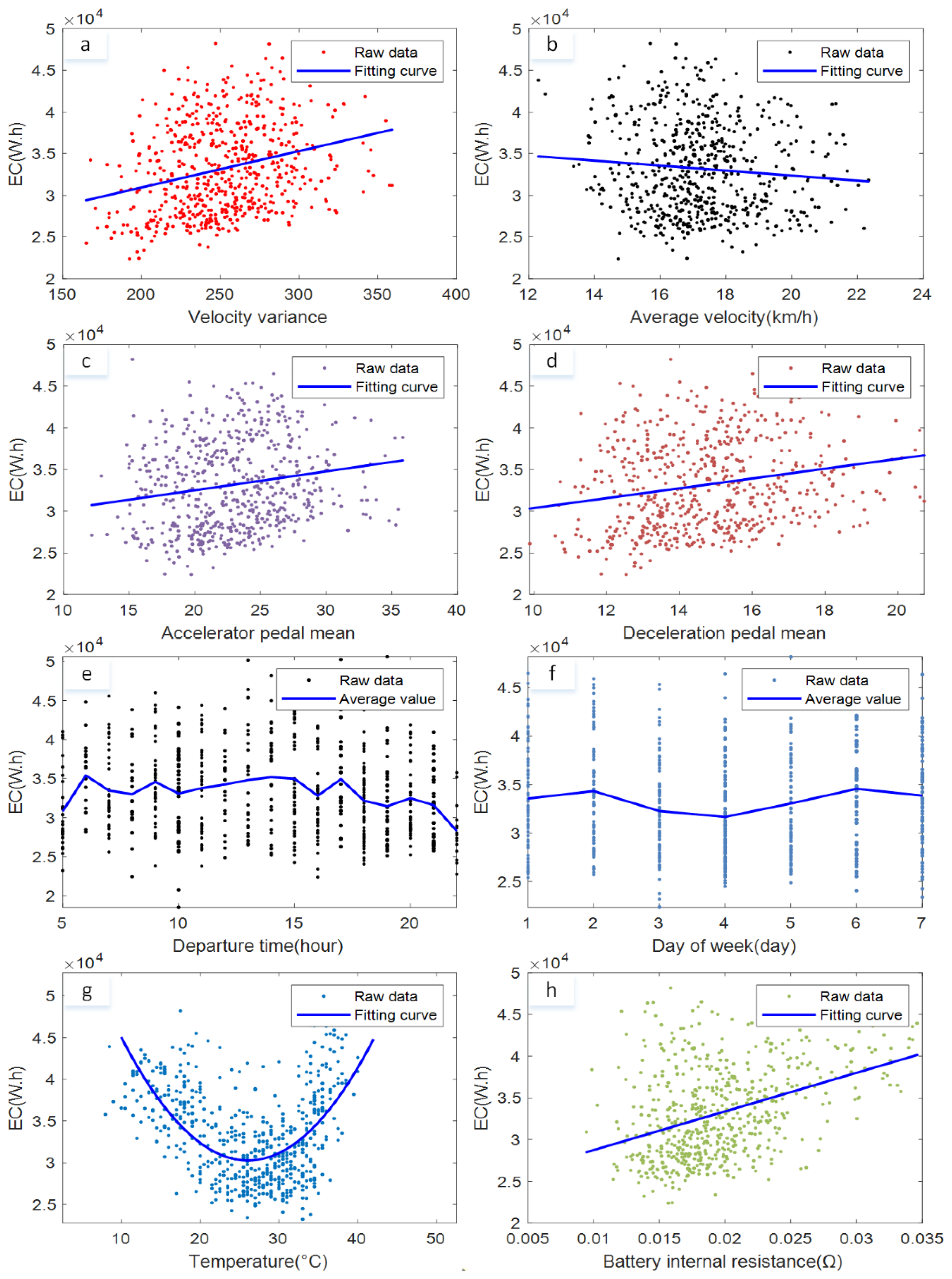
The factors that cause energy consumption fluctuations can be summarized into three aspects, including driving habits, environmental factors and vehicle performance [16]. In terms of driving habits, vehicle velocity, acceleration and deceleration conditions can cause fluctuations in vehicle energy consumption. The conditions can be quantified accordingly as the average vehicle velocity, vehicle velocity variance and number of accelerator pedal presses. In terms of the environmental factors, temperature, which is related to the energy transfer efficiency and air-conditioning usage, is the main factor causing fluctuations in vehicle energy consumption. In addition, the road conditions can also cause fluctuations in energy consumption, such as whether the departure time is congested and whether the departure date is on the weekend [17]. In terms of vehicle performance, the energy efficiency of the battery storage system during the charging and discharging process can also cause energy consumption fluctuations. The energy efficiency is mainly affected by the internal resistance of the battery system and is directly related to the ambient temperature and battery aging. Based on the analysis, the statistical results of the impact of various energy consumption fluctuation factors on vehicle energy consumption are shown in Figure 3. In the figure, it should be noted that the fitting curves were obtained by fitting experimental data with polynomial functions.
It can be seen in Figure 3a,c,d that there are positive correlations between the velocity variance, acceleration pedal statistical parameter, deceleration pedal statistical parameter and vehicle energy consumption. In Figure 3b, there is no clear correlation between the average velocity and the change in vehicle energy consumption. According to a study in the literature [8], a negative correlation between vehicle speed and energy consumption is found when the vehicle speed is below 45 km/h. Due to the large number of stopping and idling situations during the driving of electric buses, when the speed is low, the energy consumption at low speed is greater than that at high speed. Figure 3e shows that the effect of temperature on vehicle energy consumption is relatively large, and the relationship can be approximated by a quadratic function. In Figure 3f,g, the difference in departure time and departure date affects vehicle energy consumption; however, at the same point in time, vehicle energy consumption fluctuates greatly. In Figure 3h, a positive correlation is shown between the internal resistance of the battery system and the energy consumption of the vehicle. Through further analysis of the internal resistance, it was found that there is a strong correlation between the internal resistance and the battery temperature. During the driving cycle, the battery internal resistance series data have great fluctuations. As a result, the internal resistance is not taken as an input feature.
Based on the statistical analysis of the fluctuation factors of vehicle energy consumption, the main influencing features of vehicle energy consumption fluctuation are: velocity variance, average velocity, accelerator pedal parameter, deceleration pedal parameter, temperature and battery internal resistance. Considering that the internal resistance of the battery is mainly affected by the ambient temperature, the influencing features, except the internal resistance of the battery, are regarded as input features in the data-driven model.
3.2.2. Principle of CatBoost Modeling
In this paper, the CatBoost modeling approach is used to model fluctuations in vehicle energy consumption. CatBoost is an improvement of the gradient boosting decision tree (GBDT) model [18]. The approach has the ability to improve the estimation accuracy with weak learners. Moreover, it has significant advantages in extracting important features and processing categorical features. In addition, the problem of poor model accuracy and overfitting can be avoided when the dataset is uneven. The main principle of this method is to construct many weak learners for training. The weights of the training samples are adjusted to focus on samples with large estimation errors and train the weak learners in turn. Finally, the weak learners are combined into a stronger learner model [19]. In the following content, the gradient boosting decision tree algorithm is introduced. Then, the optimization strategy of the CatBoost modeling approach is given. On the basis of the modeling approach, the vehicle’s fluctuating energy consumption results can be obtained.
1. Gradient boosting decision tree
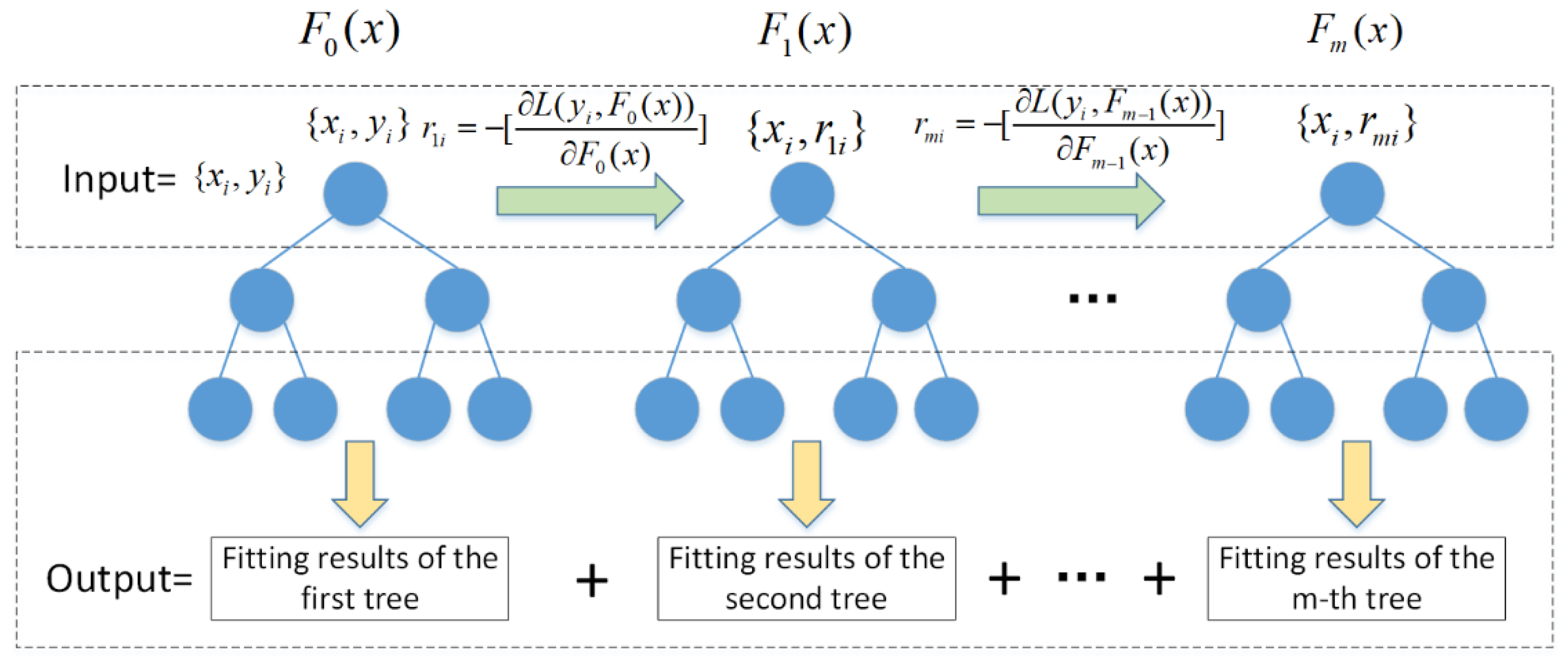
Gradient boosting decision tree is an iterative decision tree algorithm. The algorithm is composed of multiple decision trees, and the results of all trees are accumulated to obtain the final result [20]. Given a training dataset , is the characteristic affecting energy consumption, and is the predicted energy consumption of output. The goal of GBDT is to find a function that minimizes the given loss function . is accumulated by a series of decision trees . Each decision tree is optimized as:
where is the decision tree function. is the weight of the decision tree function . The initial value of can be obtained by:
Subsequently, the optimization process of the model is achieved by minimizing the loss functions:
The gradient descent method is used to solve the above optimization problems. For each model , a new dataset is constructed and trained to obtain . can be obtained by:
The value of is subsequently computed by solving a line search optimization problem. Its training process is shown in Figure 4.
2. The CatBoost modeling approach
CatBoost is a kind of gradient-enhanced decision tree algorithm, which can handle category features well [21]. The variables extracted in this paper have certain category features. Therefore, CatBoost was selected for energy consumption modeling. This method differs from GBDT in the following ways [22]:
(1) CatBoost can process features during training [23]. First, the sample data are randomly sorted to generate multiple groups of random sequences. Then, for each random sequence, the average value of the same sample is calculated. When the sequence is , it can be calculated by:
where is an a priori value. For regression tasks, the prior value is the average value in the label. is the weight of .
(2) Feature combination. The numerical features calculated by Equation (12) may lose some information. Combining features can solve this problem and produce a more effective feature. CatBoost uses a greedy approach to consider feature combinations. The first segmentation does not consider the combination of category features, and the subsequent segmentation considers all feature combinations. CatBoost takes both groups of values after segmentation as category features to participate in the following combination.
In the previous sections, the fluctuation factors of vehicle energy consumption are analyzed. Seven features can be obtained that are related to vehicle energy consumption. Based on a full understanding of the factors and the CatBoost modeling approach, features such as average vehicle velocity, vehicle velocity variance, number of accelerator pedal presses, number of brake pedal presses, departure time, day of the week and temperature, mentioned in Section 3.2.1, are taken as the input features of the CatBoost decision tree model. The statistical range of input vehicle features is a round trip of the vehicle. After model parameter optimization, the data-driven model of energy consumption can be obtained.
3.3. A Fusion of Physical and Data-Driven Models
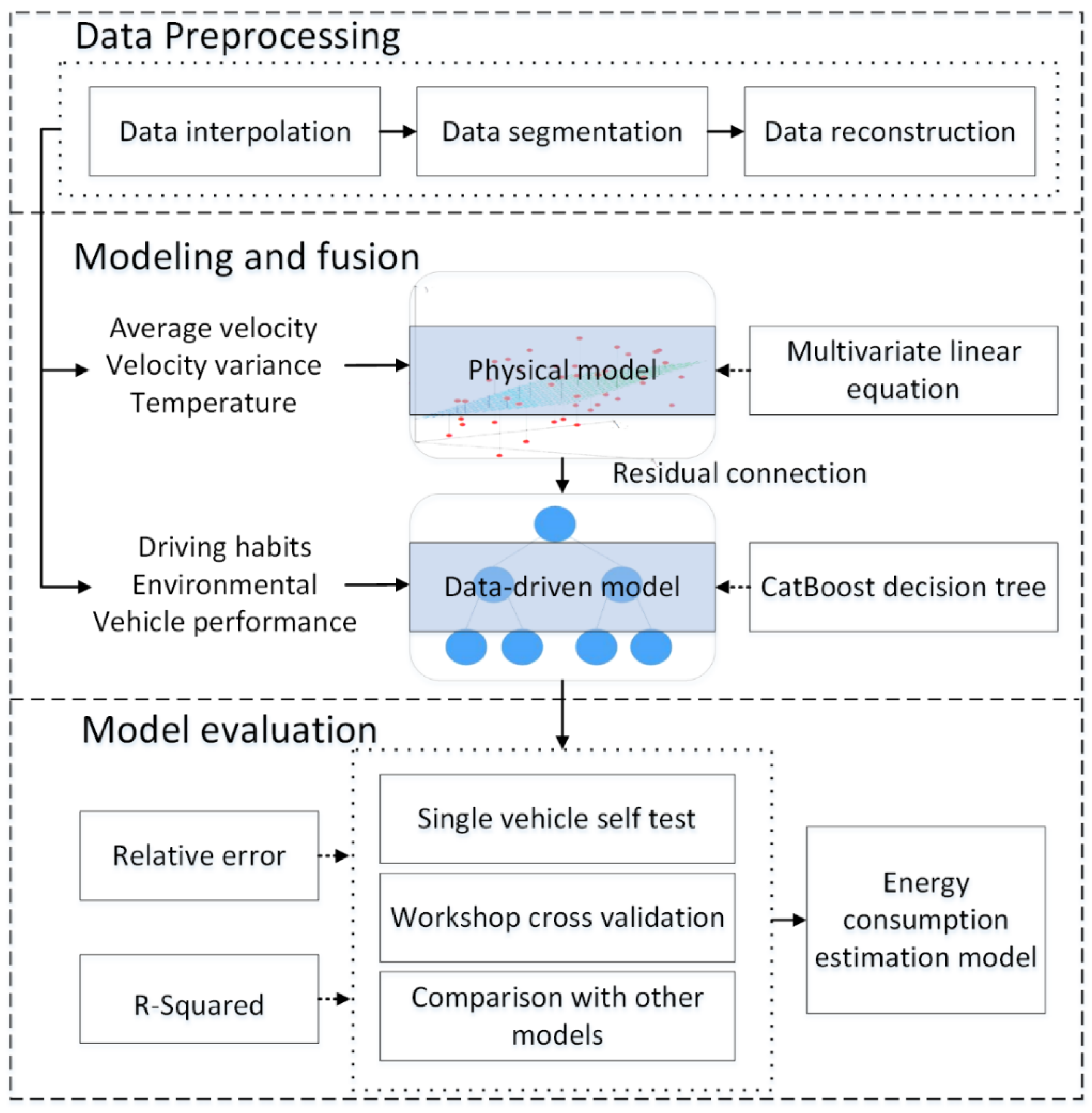
After physical and data-driven modeling of the basic energy consumption and fluctuating energy consumption of electric buses, the two parts needed to be fused to obtain a vehicle energy consumption model. In this study, the integrated learning approach in machine learning theory was used for model fusion. The reconstructed electric bus data were used to train the physical energy consumption model. The residual of the basic model was retrained as the training label of the data-driven model [24]. The flow chart of the energy consumption fusion modeling approach is shown in Figure 5.
The modeling approach can be divided into three steps:
(1) Data processing. In this process, the original data are interpolated. For different missing data types, the methods of average interpolation and Lagrange interpolation are adopted. For outliers in the data, the method of constructing quartile positions with a box plot is used to remove them. Then, the data are segmented according to the state of charge. After the specific driving segments are divided, data such as vehicle speed, data acquisition time, temperature, accelerator pedal value and deceleration pedal value can be obtained. The data are further processed for energy consumption modeling.
(2) Modeling and fusion. The original features obtained from the data processing step include vehicle speed, data acquisition time, temperature, accelerator pedal value and deceleration pedal value. These features need to be processed separately and input into the model. For the physical model, the vehicle driving distance, speed variance and the square of the difference between the temperature in the vehicle and the standard temperature are calculated as inputs. For the data-driven model, the departure time of the vehicle, whether it is a weekend, the temperature in the vehicle, the value of acceleration and deceleration pedal, the average speed and the speed variance are extracted and input into the CatBoost model. In engineering applications, many specific data in vehicle operation are unknown. Therefore, the input of the model needs to meet the following conditions: (1) The input parameters of the model can be obtained before the vehicle is driven. (2) The input parameters of the model need to include parameters that reflect the working condition information. This paper simplifies the input parameters according to this criterion and obtains the following input parameters: the mileage of the current route, the average speed, the speed variance, the temperature, the air-conditioning condition, the departure time, the departure day of the week and the average values of the accelerator pedal and the deceleration pedal. These parameters can be planned before driving. The aim of the fusion step of the model is to train the physical model to obtain the preliminary estimation results of energy consumption. Then, the residual of the physical model is retrained as the training label of the data-driven model to minimize the residual. The final energy consumption result is the sum of the results of the two models.
(3) Model evaluation. Two indicators are selected for the verification of model results, namely, the average relative error and the R-squared parameter. The verification is divided into a single vehicle division training set and a test set for verification. In order to test the robustness of the model, different vehicles are selected for verification.
4. Results and Discussions
4.1. Analysis of the Results of the Physical Model
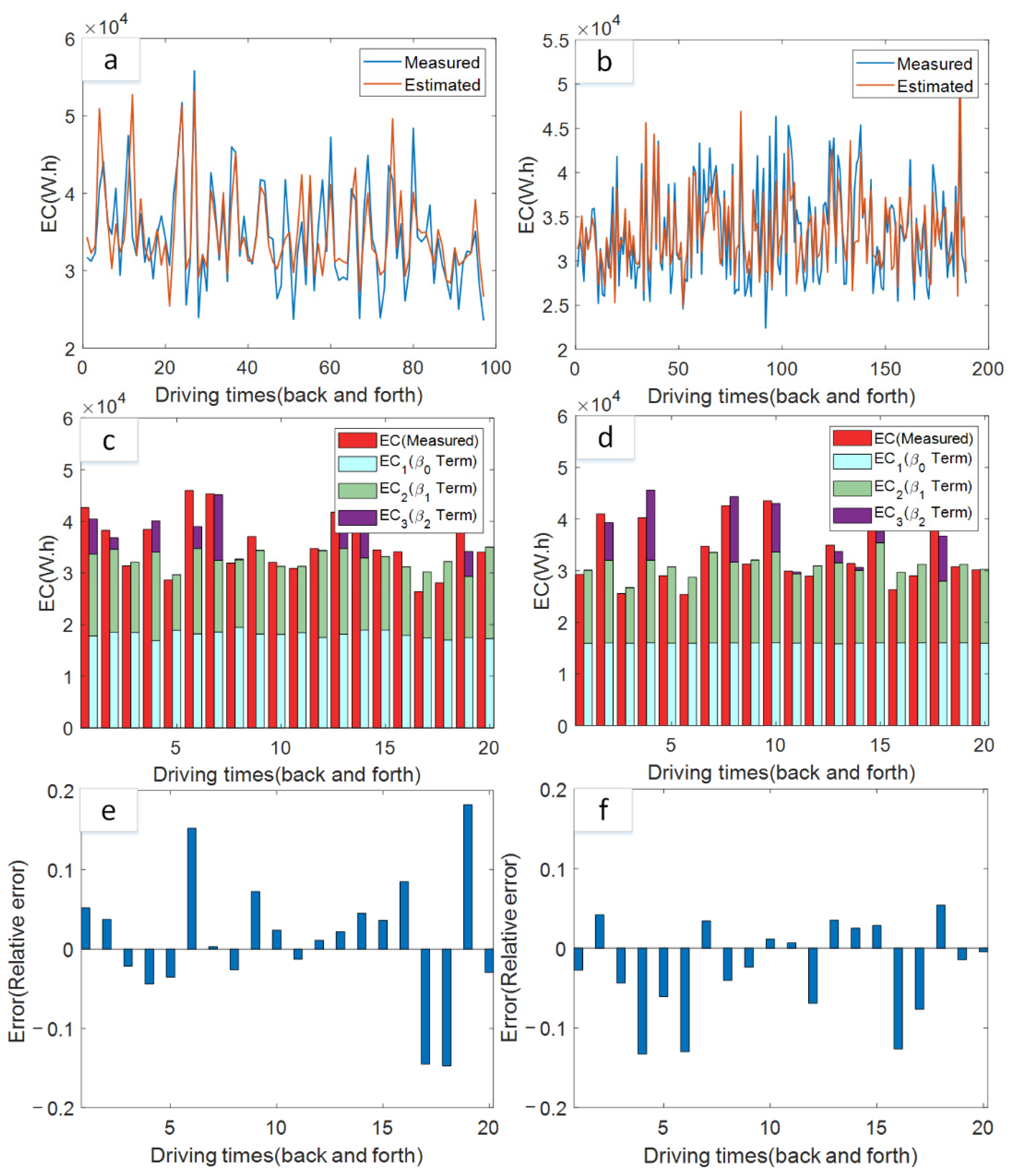
The physical model to obtain the basic energy consumption was analyzed. In this work, data provided by the new energy vehicle big data platform were used for model training. The parameters of the physics-based basic energy consumption model of six electric buses were estimated. The results are shown in Table 2. Figure 6 shows the basic energy consumption estimation results of two electric buses (Bus 1 and Bus 2). As a large number of data points can cause the bar chart to be too small, only 20 points in Figure 6a,b were used to draw Figure 6c–f.
It can be seen that the vehicle’s rolling drag energy consumption coefficient is the largest. This shows that the main energy consumption of the vehicle during driving is consumed by the rolling drag. In the figure, Figure 6a,b compare the fitted values of the model with the real values of vehicle energy consumption. In the figure, the x-axis represents the number of vehicle round trips, and the y-axis represents the energy consumption. The model-fitting results are close to the values in terms of vehicle energy consumption data. Figure 6c,d show the proportion of the energy consumption of each component in the total energy consumption as a histogram. It is obvious that rolling drag and kinetic energy change dominate the energy consumption. Since the use of an air conditioner is closely related to the temperature difference between inside and outside the vehicle, the energy consumption data of the air conditioner fluctuate greatly. The errors of the basic energy consumption model are shown in Figure 6e,f. It can be seen that the average error of the estimation results is 7%. Since the model does not consider the influence of energy consumption fluctuations, there are large errors in the estimation of vehicle energy consumption.
4.2. Analysis of the Results of the Fusion Model
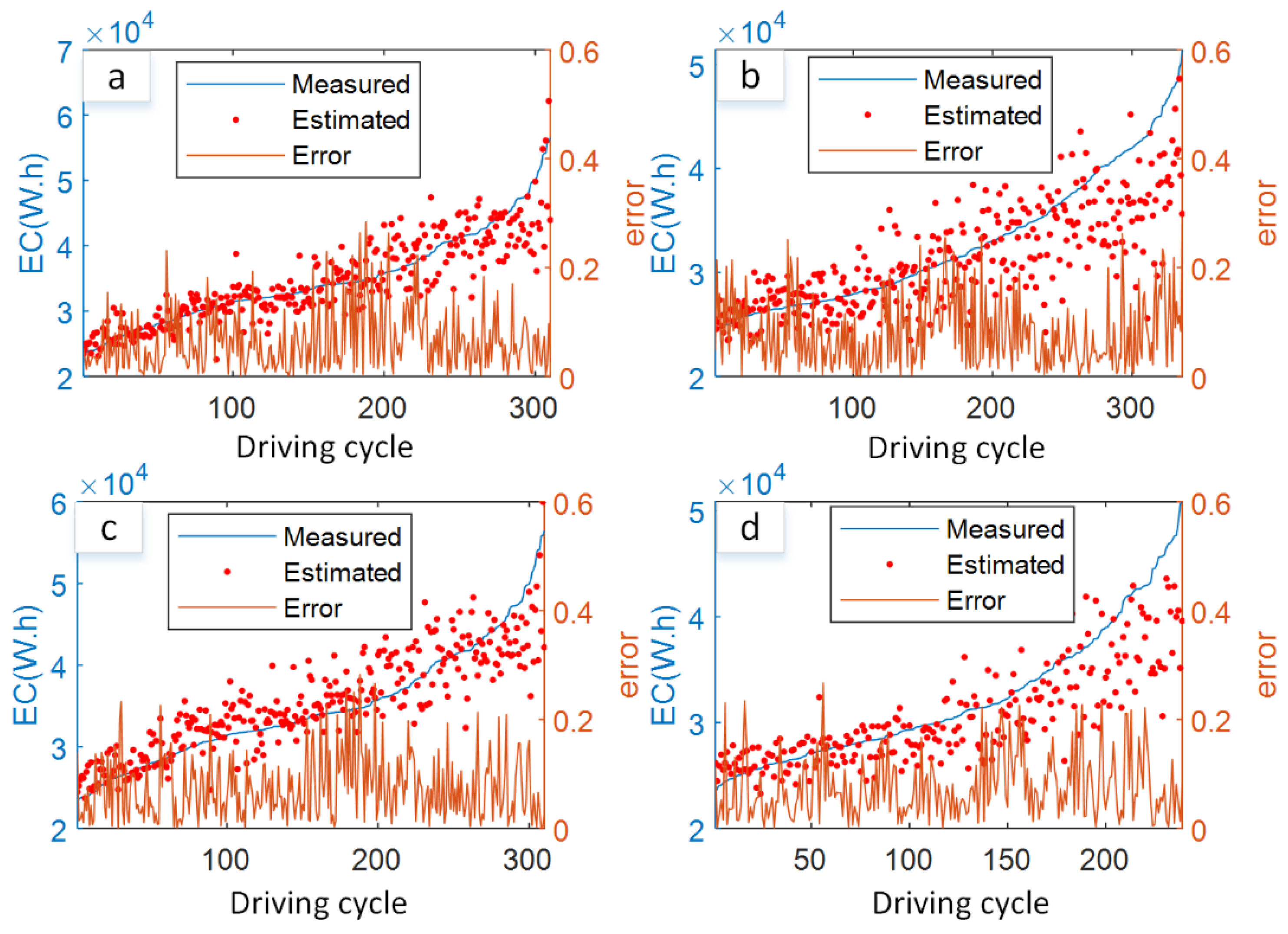
The energy consumption estimation results obtained from the physical energy consumption model only take into account energy consumption in ideal conditions. The model does not account for the influence of driving habits and environmental factors. In this context, the physical model and the data-driven model are fused to estimate vehicle energy consumption. The results of the vehicle energy consumption estimation of the fusion model are shown in Figure 7.
In Figure 7, the blue line represents the vehicle energy consumption obtained using the platform data, which can be considered a reference value for the vehicle energy consumption. The red points are the vehicle energy consumption obtained by the fusion model. It is clear that the estimation results of vehicle energy consumption are able to track changes in the real energy consumption of the vehicle with small estimation errors. The relative error of the fusion model on the Bus 1 dataset is 4.8%. However, not all results performed well. In some cases, the error reaches 15%. When the data were analyzed separately, it can be found that the larger errors occurred mainly during morning peaks and severe weather periods. Modeling these situations is complex and beyond the scope of this paper. To verify the generalizability capability of the model, two buses (Bus 1 and Bus 2) were selected as training samples, and other vehicle data were used as test data.
The energy consumption estimation results with multi-vehicle data and the fusion model are shown in Figure 8. The results show that the energy consumption estimation errors for multiple vehicles are within 8.1%. The statistics of the estimation results for the energy consumption of the fusion model are shown in Table 3. The average error of the vehicle energy consumption estimation results is 7.5%.
4.3. Method Comparison and Verification
To further validate the effectiveness of the fusion model, several other vehicle energy consumption estimation models are introduced for comparison with the model proposed in this paper. The algorithms for comparison include the physical model, CatBoost decision tree model and fusion models with different approaches. In terms of validity assessment, the average relative error and the coefficient of determination are regarded as indicators for evaluation. The coefficient of determination is a correlation index that measures how well the data trend fits. Herein, the coefficient of determination is obtained using the R-squared method. The assessment indicators can be calculated by:
where and represent the real value and the estimated value, respectively. is the number of samples.
The results of the different energy consumption estimation models are shown in Table 4. These models were used to calculate the vehicle energy consumption in this paper. It can be seen that the physical model gives the worst energy consumption estimation results. In contrast, the CatBoost decision tree modeling approach has better estimation results. Ultimately, the physical-CatBoost decision tree model gives the best estimation results, with relative errors and coefficients of determination of 6.1% and 0.79, respectively.
The complexity of the Physics-CatBoost fusion model was tested. One million pieces of data were processed on a computer with Intel® core™ i5-10400 CPU @ 2.90 GHz running memory of 32 GB (Santa Clara, CA, USA). The data processing time was 6 s, and the model training time was only 0.9 s. It can be seen that the complexity of the model is low.
5. Conclusions
This research focused on the energy consumption estimation of electric buses based on a physical and data-driven fusion model. In terms of physical modeling, a basic energy consumption model was constructed. Rolling drag, kinetic energy consumption and air-conditioning factors were considered. In terms of data-driven modeling, the main factors affecting the fluctuation of vehicle energy consumption were studied. The input characteristics of the model were simplified so that the input of the model can be built before vehicle driving. A CatBoost decision tree modeling approach was employed to construct the model for estimating fluctuating energy consumption. In the model training process, the idea of integrated learning was utilized to optimize the model in a hierarchical iteration. The results show that the average relative error of the vehicle energy consumption estimation result is 6.1%. The coefficient of determination is 0.79. Compared with other energy consumption modeling methods, the fusion model performs best with the two indicators. The fusion model proposed in this paper has better accuracy and generalization ability than other models. It provides a reference basis for the optimization of the energy consumption of electric buses, vehicle scheduling and the rational layout of charging stations.
Based on the results, most of the points with large errors are concentrated in bad weather. In order to further improve the accuracy of the model, weather factors can be added to the model in the future. In addition, vehicle mass is regarded as a constant value in the driving process, which is also a reason for the model error. Therefore, the establishment of the dynamic estimation of vehicle mass in a follow-up work can improve the accuracy of the model.
Author Contributions
Conceptualization, X.L. and T.W.; methodology, X.L.; software, T.W.; validation, T.W. and J.L.; formal analysis, X.L. and T.W.; investigation, T.W. and J.L.; resources, Y.T. and J.T.; data curation, J.T.; writing—original draft preparation, X.L. and T.W.; writing—review and editing, X.L. and J.T.; visualization, T.W.; supervision, Y.T. and J.T.; project administration, J.T.; funding acquisition, X.L. All authors have read and agreed to the published version of the manuscript.
Funding
This work was supported by the National Natural Science Foundation of China (No. 52177219) and the Natural Science Foundation of Guangdong Province (2021A1515010525).
Data Availability Statement
The National Big Data Alliance of New Energy Vehicles (NDAEV) provided research data. The source of the data is the China National New Energy Vehicle Monitoring and Management Platform.
Conflicts of Interest
The authors declare no conflict of interest. The funders had no role in the design of the study; in the collection, analyses or interpretation of data; in the writing of the manuscript; or in the decision to publish the results.
References
- Docherty, I.; Marsden, G.; Anable, J. The governance of smart mobility. Transp. Res. Part A Policy Pract. 2018, 115, 114–125. [Google Scholar] [CrossRef]
- Babu, N. Review of the Estimation Methods of Energy Consumption for Battery Electric Buses. Energies 2021, 14, 7578. [Google Scholar] [CrossRef]
- Pamuła, T.; Pamuła, W. Estimation of the energy consumption of battery electric buses for public transport networks using real-world data and deep learning. Energies 2020, 13, 2340. [Google Scholar] [CrossRef]
- Yuan, X.; Zhang, C.; Hong, G.; Huang, X.; Li, L. Method for evaluating the real-world driving energy consumptions of electric vehicles. Energy 2017, 141, 1955–1968. [Google Scholar] [CrossRef]
- Bracco, S.; Bianco, G.; Siri, S.; Barbagelata, C.; Casati, C.; Siri, E. Simulation Models for the Evaluation of Energy Consumptions of Electric Buses in Different Urban Traffic Scenarios. In Proceedings of the 2021 Sixteenth International Conference on Ecological Vehicles and Renewable Energies (EVER), Monte-Carlo, Monaco, 5–7 May 2021; pp. 1–6. [Google Scholar] [CrossRef]
- Qi, X.; Wu, G.; Boriboonsomsin, K.; Barth, M.J. Data-driven decomposition analysis and estimation of link-level electric vehicle energy consumption under real-world traffic conditions. Transp. Res. Part D Transp. Environ. 2018, 64, 36–52. [Google Scholar] [CrossRef] [Green Version]
- Hao, X.; Wang, H.; Lin, Z.; Ouyang, M. Seasonal effects on electric vehicle energy consumption and driving range: A case study on personal, taxi, and ridesharing vehicles. J. Clean. Prod. 2020, 249, 119403. [Google Scholar] [CrossRef]
- Miraftabzadeh, S.M.; Longo, M.; Foiadelli, F. Estimation Model of Total Energy Consumptions of Electrical Vehicles under Different Driving Conditions. Energies 2021, 14, 854. [Google Scholar] [CrossRef]
- Al-Wreikat, Y.; Serrano, C.; Sodré, J.R. Effects of ambient temperature and trip characteristics on the energy consumption of an electric vehicle. Energy 2022, 238, 122028. [Google Scholar] [CrossRef]
- Björnsson, L.H.; Karlsson, S. The potential for brake energy regeneration under Swedish conditions. Appl. Energy 2016, 168, 75–84. [Google Scholar] [CrossRef] [Green Version]
- Ritari, A.; Tammi, K.; Laitinen, H. Energy Consumption and Lifecycle Cost Analysis of Electric City Buses with Multispeed Gearboxes. Energies 2020, 13, 2117. [Google Scholar] [CrossRef]
- Li, X.; Wang, T.; Wu, C.; Tian, J.; Tian, Y. Battery Pack State of Health Prediction Based on the Electric Vehicle Management Platform Data. World Electr. Veh. J. 2021, 12, 204. [Google Scholar] [CrossRef]
- De Cauwer, C.; Van Mierlo, J.; Coosemans, T. Energy consumption prediction for electric vehicles based on real-world data. Energies 2015, 8, 8573–8593. [Google Scholar] [CrossRef]
- Kanarachos, S.; Mathew, J.; Fitzpatrick, M.E. Instantaneous vehicle fuel consumption estimation using smartphones and recurrent neural networks. Expert Syst. Appl. 2019, 120, 436–447. [Google Scholar] [CrossRef]
- Li, W. Modeling and Energy Consumption Proportion Analysis of Pure Electric Vehicle Air Conditioning System; Jilin University: Changchu, China, 2020. [Google Scholar] [CrossRef]
- Vepsäläinen, J.; Otto, K.; Lajunen, A.; Tammi, K. Computationally efficient model for energy demand prediction of electric city bus in varying operating conditions. Energy 2019, 169, 433–443. [Google Scholar] [CrossRef]
- Qin, W.; Wang, L.; Liu, Y.; Xu, C. Energy Consumption Estimation of the Electric Bus Based on Grey Wolf Optimization Algorithm and Support Vector Machine Regression. Sustainability 2021, 13, 4689. [Google Scholar] [CrossRef]
- Truong, V.H.; Vu, Q.V.; Thai, H.T.; Ha, M.H. A robust method for safety evaluation of steel trusses using Gradient Tree Boosting algorithm. Adv. Eng. Softw. 2020, 147, 102825. [Google Scholar] [CrossRef]
- Zhang, T.; He, W.; Zheng, H.; Cui, Y.; Song, H.; Fu, S. Satellite-based ground PM2.5 estimation using a gradient boosting decision tree. Chemosphere 2021, 268, 128801. [Google Scholar] [CrossRef] [PubMed]
- Bentéjac, C.; Csörgő, A.; Martínez-Muñoz, G. A comparative analysis of gradient boosting algorithms. Artif. Intell. Rev. 2020, 54, 1937–1967. [Google Scholar] [CrossRef]
- Jabeur, S.B.; Gharib, C.; Mefteh-Wali, S.; Arfi, W.B. CatBoost model and artificial intelligence techniques for corporate failure prediction. Technol. Forecast. Soc. Chang. 2021, 166, 120658. [Google Scholar] [CrossRef]
- Huang, G.; Wu, L.; Ma, X.; Zhang, W.; Fan, J.; Yu, X.; Zhou, H. Evaluation of CatBoost method for prediction of reference evapotranspiration in humid regions. J. Hydrol. 2019, 574, 1029–1041. [Google Scholar] [CrossRef]
- Prokhorenkova, L.; Gusev, G.; Vorobev, A.; Dorogush, A.V.; Gulin, A. CatBoost: Unbiased boosting with categorical features. Adv. Neural Inf. Process. Syst. 2018, 31, 1–11. Available online: https://proceedings.neurips.cc/paper/2018/file/14491b756b3a51daac41c24863285549-Paper.pdf (accessed on 1 December 2018).
- Sivadas, N.; Okamoto, S.; Xu, X.; Fennie, C.J.; Xiao, D. Stacking-dependent magnetism in bilayer CrI3. Nano Lett. 2018, 18, 7658–7664. [Google Scholar] [CrossRef] [PubMed] [Green Version]
Figure 1.
Electric bus operation data transmission and preprocessing results. (a) Driving route, (b) electric vehicle big data cloud platform and (c) preprocessing results of battery SOC.
Figure 1.
Electric bus operation data transmission and preprocessing results. (a) Driving route, (b) electric vehicle big data cloud platform and (c) preprocessing results of battery SOC.

Figure 2.
Statistical results of vehicle energy consumption after reconstruction. The relationships of (a) temperature, (b) vehicle velocity variance, (c) average velocity and (d) departure time with vehicle energy consumption.
Figure 2.
Statistical results of vehicle energy consumption after reconstruction. The relationships of (a) temperature, (b) vehicle velocity variance, (c) average velocity and (d) departure time with vehicle energy consumption.

Figure 3.
The statistical results of the impact of various energy consumption fluctuation factors on vehicle energy consumption. (a–h) The relationships between the velocity variance, average velocity, number of accelerator pedal presses, number of deceleration pedal presses, departure time, departure date, ambient temperature, internal resistance of the battery pack and energy consumption, respectively.

Figure 4.
The training process of the gradient boosting decision tree modeling approach.

Figure 5.
Flow chart of the energy consumption fusion modeling approach.

Figure 6.
The basic energy consumption estimation results. (a,b) The fitting curves of two electric buses. (c,d) The energy consumption fitting results for each part. (e,f) The fitting errors.
Figure 6.
The basic energy consumption estimation results. (a,b) The fitting curves of two electric buses. (c,d) The energy consumption fitting results for each part. (e,f) The fitting errors.

Figure 7.
Energy consumption estimation results with the fusion model. (a–d) Bus 1 to Bus 4.

Figure 8.
Energy consumption estimation results with multi-vehicle data and the fusion model. (a–d) Bus 1 to Bus 4.
Figure 8.
Energy consumption estimation results with multi-vehicle data and the fusion model. (a–d) Bus 1 to Bus 4.


Table 1.
A detailed description of the items used in this paper.
| Item | Type | Explain |
|---|---|---|
| VIN | STRING | Vehicle identification number |
| State of charge | INT | Parking charging, driving charging, not charging, charging completed, abnormal, invalid |
| Speed | FLOAT | 0~220 (km/h), abnormal |
| Cumulative travel | FLOAT | 0~999,999.9 (km), abnormal |
| Total voltage | FLOAT | 0~1000 (V), abnormal |
| Total current | FLOAT | −1000~1000 (A), abnormal |
| SOC | INT | 0~100(%), abnormal |
| Temperature | INT | −40~210 (°C), abnormal |
| Accelerator pedal | INT | 0~100, abnormal |
| Deceleration pedal | INT | 0~100, abnormal |
| Data acquisition time | STRING | Time of each data acquisition |
Table 2.
Parameters of the physical model.
| Vehicle Number | β0 | β1 | β2 |
|---|---|---|---|
| Bus 1 | 884.5 | 14.2 | 47.1 |
| Bus 2 | 869.3 | 11.3 | 64.3 |
| Bus 3 | 810.0 | 11.7 | 71.1 |
| Bus 4 | 855.7 | 11.3 | 76.2 |
| Bus 5 | 775.4 | 16.6 | 59.5 |
| Bus 6 | 866.3 | 2.3 | 88.5 |
| Average | 843.6 | 11.2 | 67.7 |
Table 3.
The statistics of the estimation results for energy consumption of the fusion model.
| Vehicle Number | Relative Error of Vehicle Self-Test | R-Squared of Vehicle Self-Test | Relative Error of Other Vehicles | R-Squared of Other Vehicles |
|---|---|---|---|---|
| Bus 1 | 4.8% | 0.83 | Training vehicle | Training vehicle |
| Bus 2 | 5.5% | 0.82 | Training vehicle | Training vehicle |
| Bus 3 | 6.6% | 0.75 | 7.5% | 0.67 |
| Bus 4 | 6.9% | 0.76 | 7.7% | 0.63 |
| Bus 5 | 5.9% | 0.77 | 7.0% | 0.74 |
| Bus 6 | 7.0% | 0.78 | 8.1% | 0.61 |
| Average | 6.1% | 0.79 | 7.5% | 0.66 |
Table 4.
Vehicle energy consumption estimation results with different models.
| Model | Average Relative Error of Vehicle | Average R-Squared of Vehicle |
|---|---|---|
| Physical model | 8.4% | 0.66 |
| CatBoost model | 7.0% | 0.72 |
| Physics-Neural network model | 6.8% | 0.72 |
| Physics-Random forest model | 6.8% | 0.73 |
| Physics-XGBoost model | 6.9% | 0.73 |
| Physics-CatBoost fusion model | 6.1% | 0.79 |
Publisher’s Note: MDPI stays neutral with regard to jurisdictional claims in published maps and institutional affiliations. |
© 2022 by the authors. Licensee MDPI, Basel, Switzerland. This article is an open access article distributed under the terms and conditions of the Creative Commons Attribution (CC BY) license (https://creativecommons.org/licenses/by/4.0/).
Share and Cite
MDPI and ACS Style
Li, X.; Wang, T.; Li, J.; Tian, Y.; Tian, J. Energy Consumption Estimation for Electric Buses Based on a Physical and Data-Driven Fusion Model. Energies 2022, 15, 4160. https://doi.org/10.3390/en15114160
AMA Style
Li X, Wang T, Li J, Tian Y, Tian J. Energy Consumption Estimation for Electric Buses Based on a Physical and Data-Driven Fusion Model. Energies. 2022; 15(11):4160. https://doi.org/10.3390/en15114160
Chicago/Turabian StyleLi, Xiaoyu, Tengyuan Wang, Jiaxu Li, Yong Tian, and Jindong Tian. 2022. "Energy Consumption Estimation for Electric Buses Based on a Physical and Data-Driven Fusion Model" Energies 15, no. 11: 4160. https://doi.org/10.3390/en15114160
Note that from the first issue of 2016, this journal uses article numbers instead of page numbers. See further details here.