
Analyzing Intersectoral Benefits of District Heating in an Integrated Generation and Transmission Expansion Planning Model

 , , , ,
  , ,
, ,
Abstract
:
1. Introduction
1.1. Motivation
1.2. State of the Art
1.3. Contribution and Aim of this Study
2. Materials and Methods
2.1. Model
2.1.1. Generation and Transmission Expansion Planning Model
2.1.2. Enhancements for Modeling Thermal Demand
2.1.3. Heat Pumps and Electric Boilers
2.1.4. Thermal Energy Storage
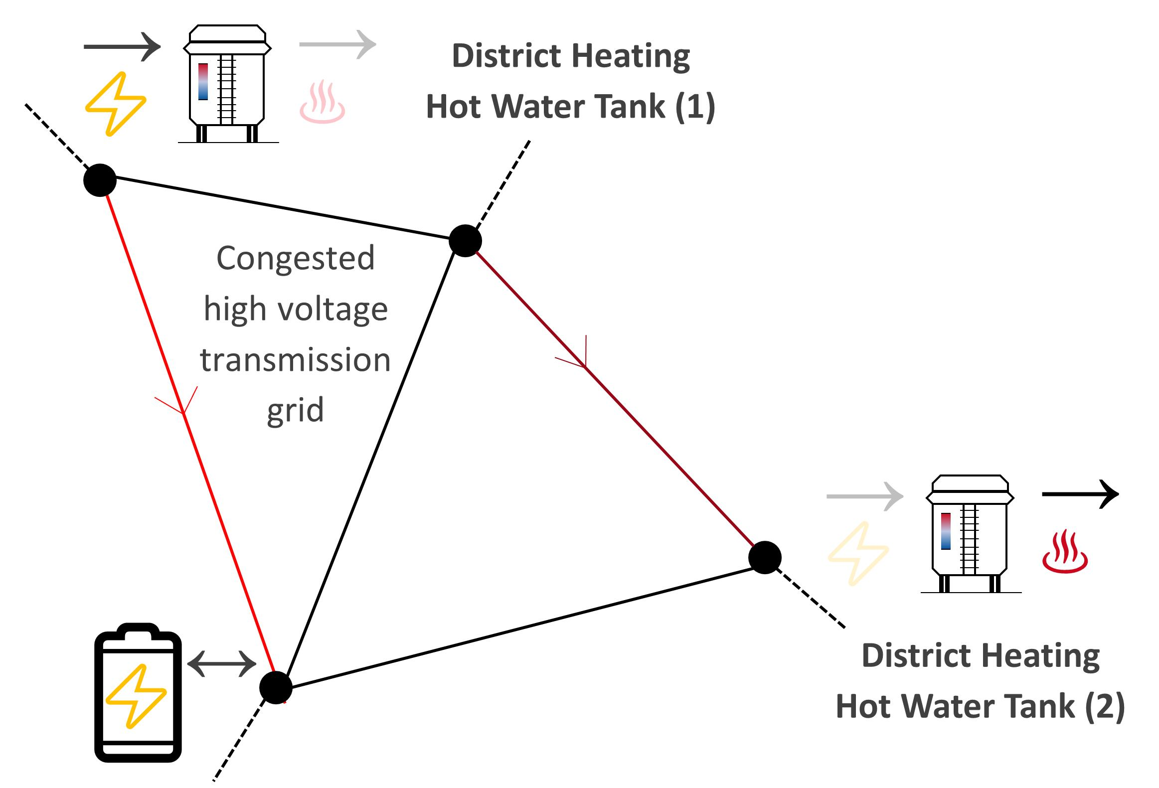
2.1.5. Combined Heat and Power
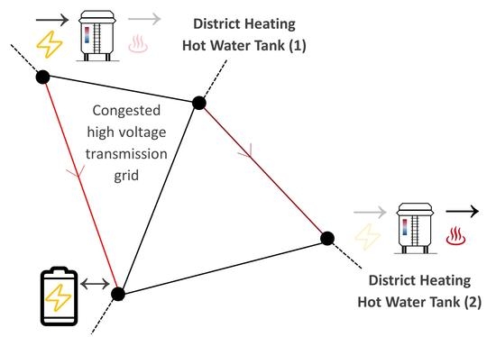
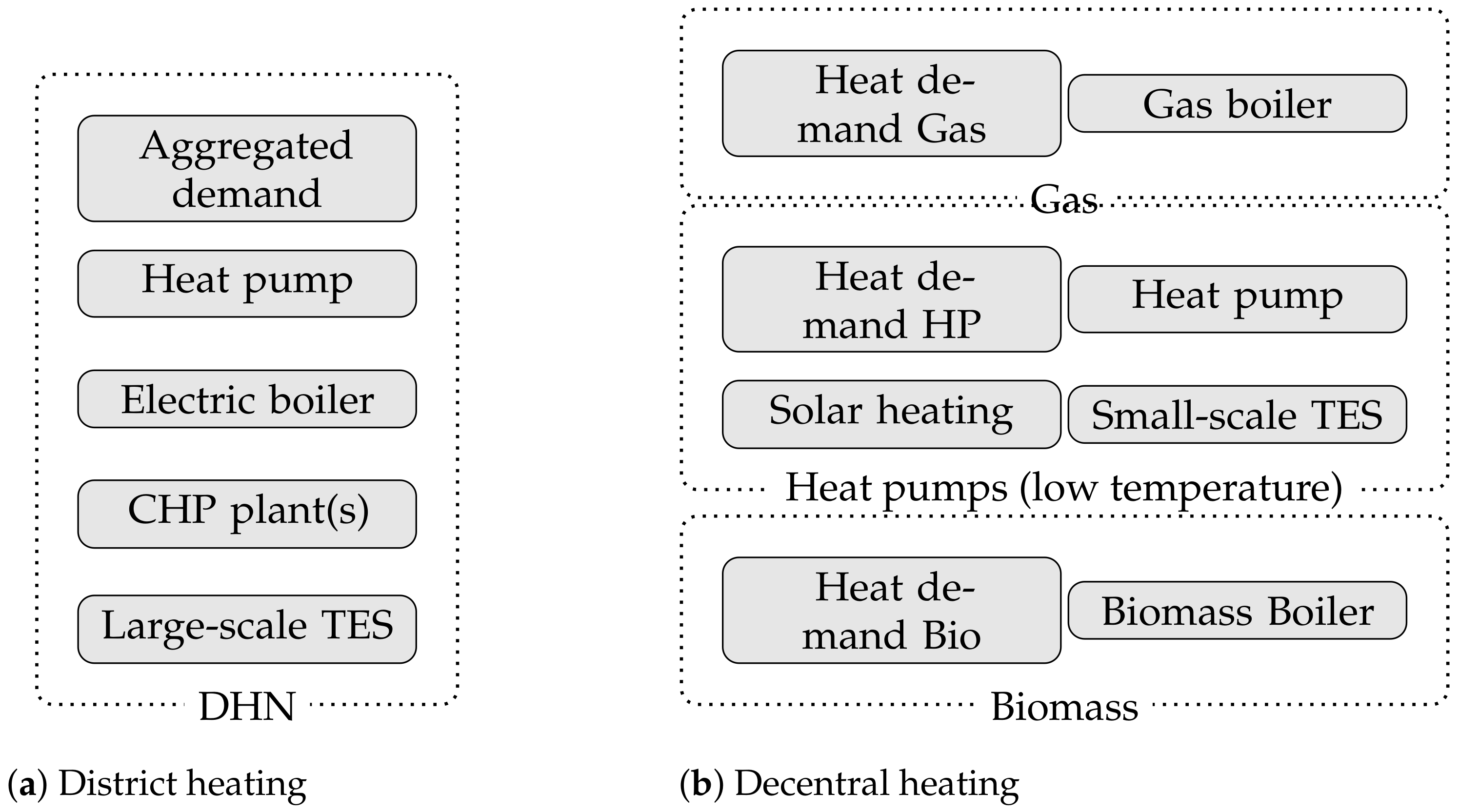
2.1.6. Modeling District Heating
2.1.7. Modeling Decentral Heating
2.2. Data
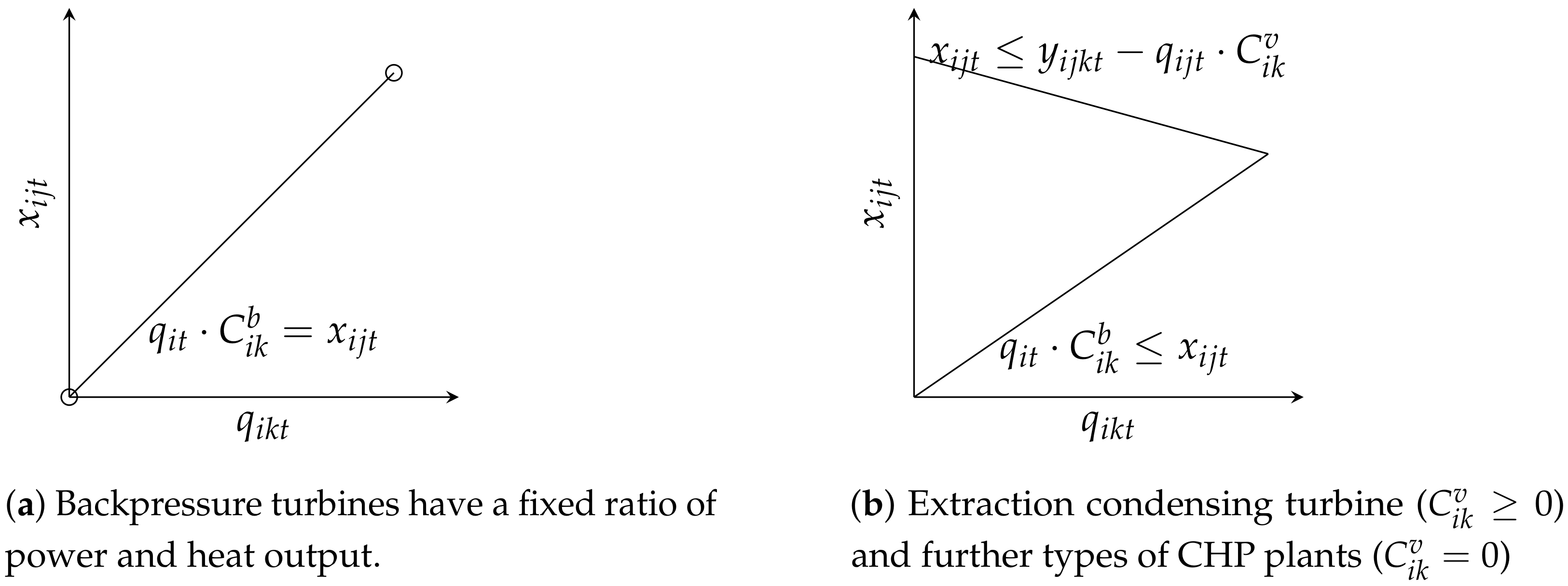
2.2.1. Focus of Investigation
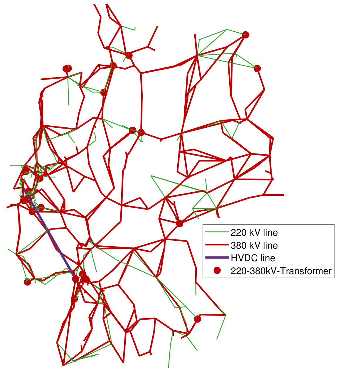
2.2.2. Network Data
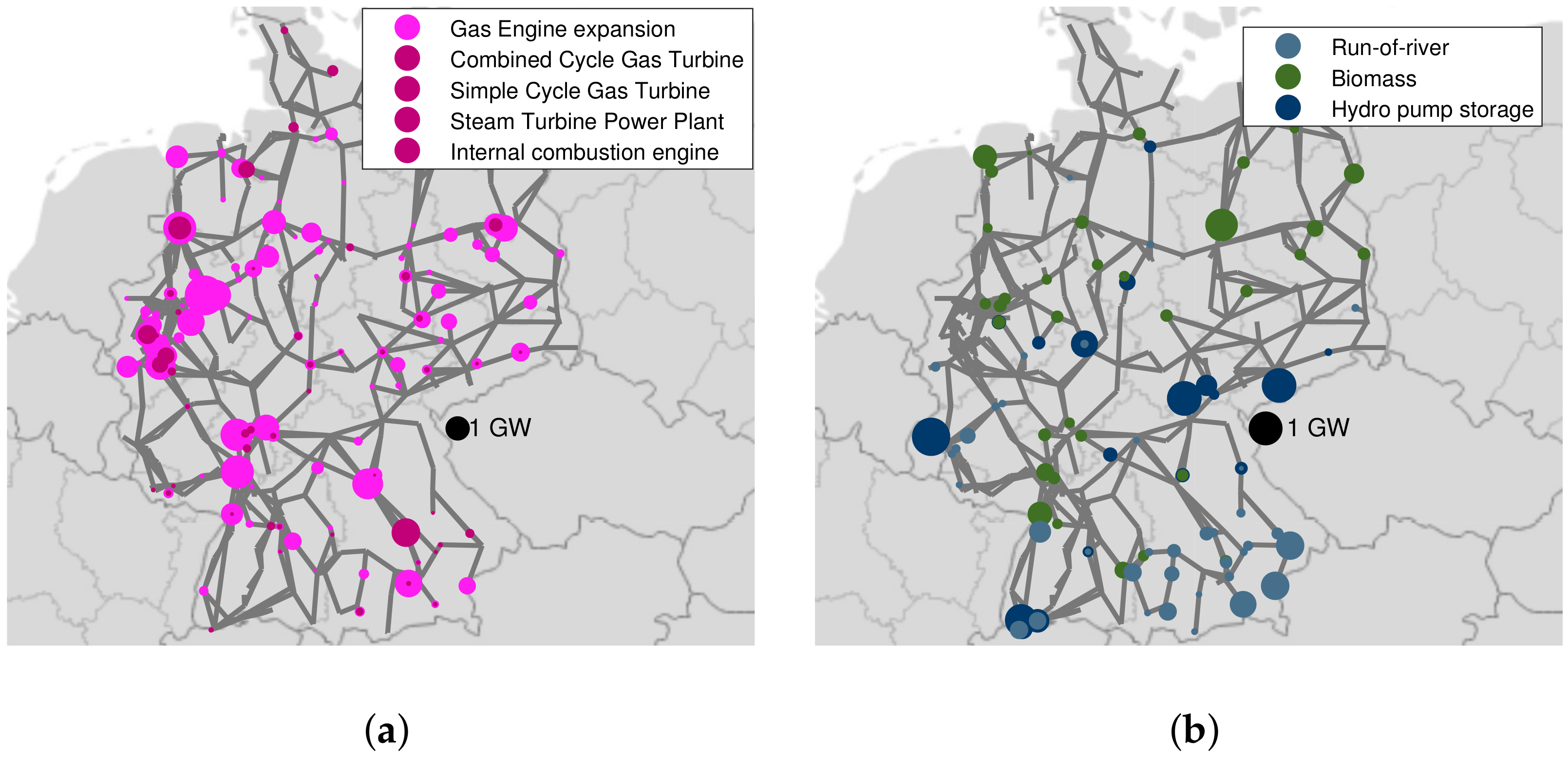
2.2.3. Conventional Power Plants
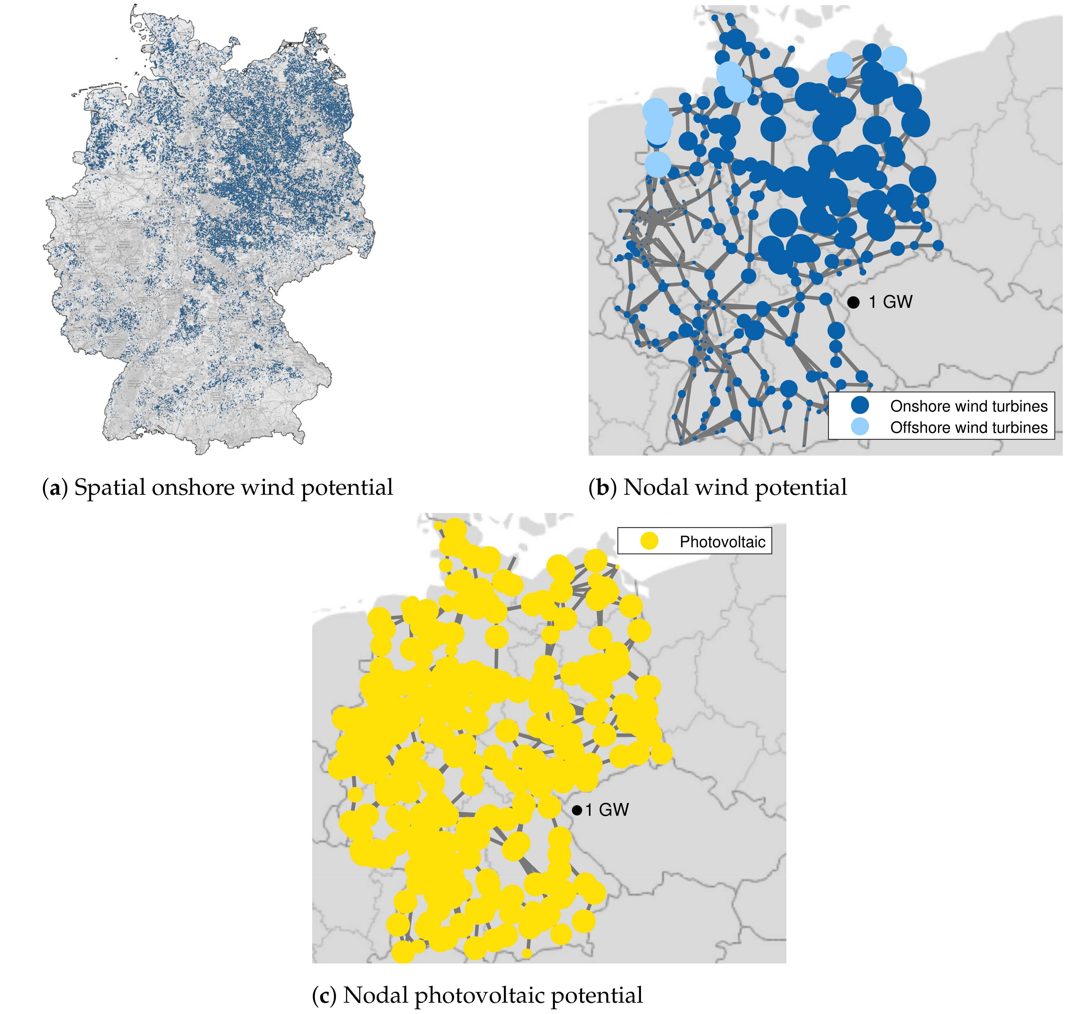
2.2.4. Renewable Feed-in Profiles and Potentials
2.2.5. New Technologies
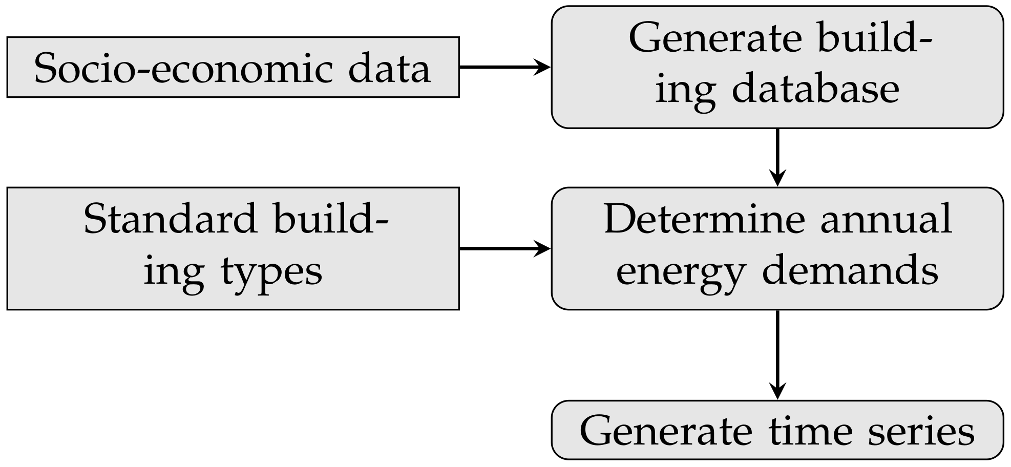
2.2.6. Bottom-Up Regionalization of Demand Data
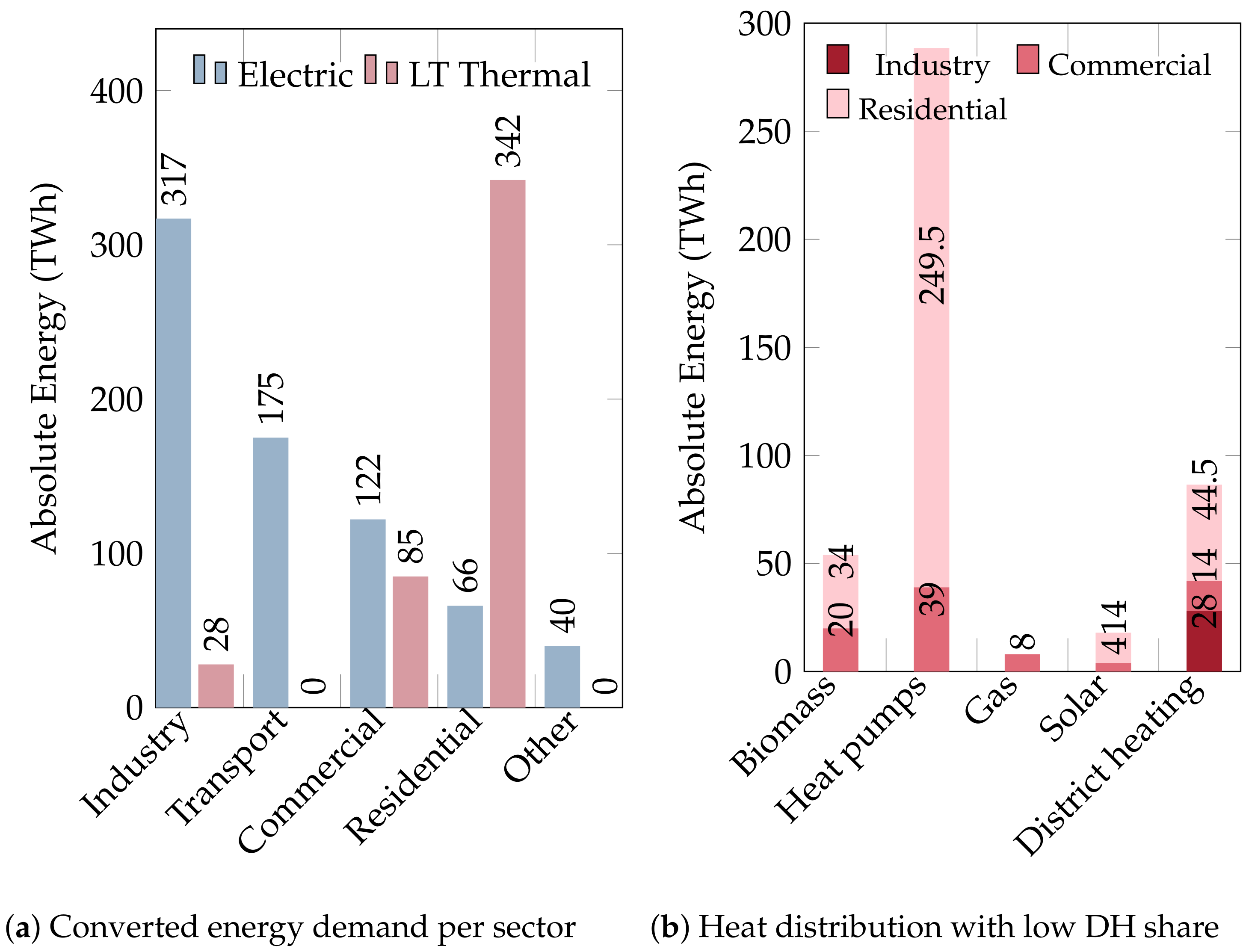
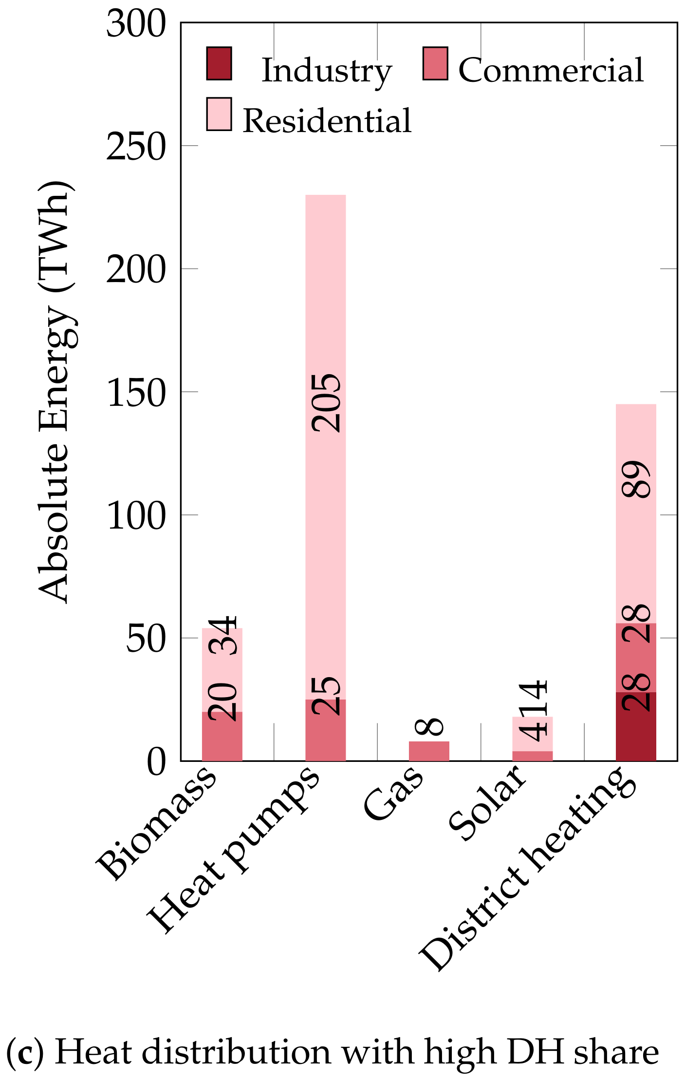
2.2.7. Energy Demand, and Sensitivities
3. Results
3.1. Calculation
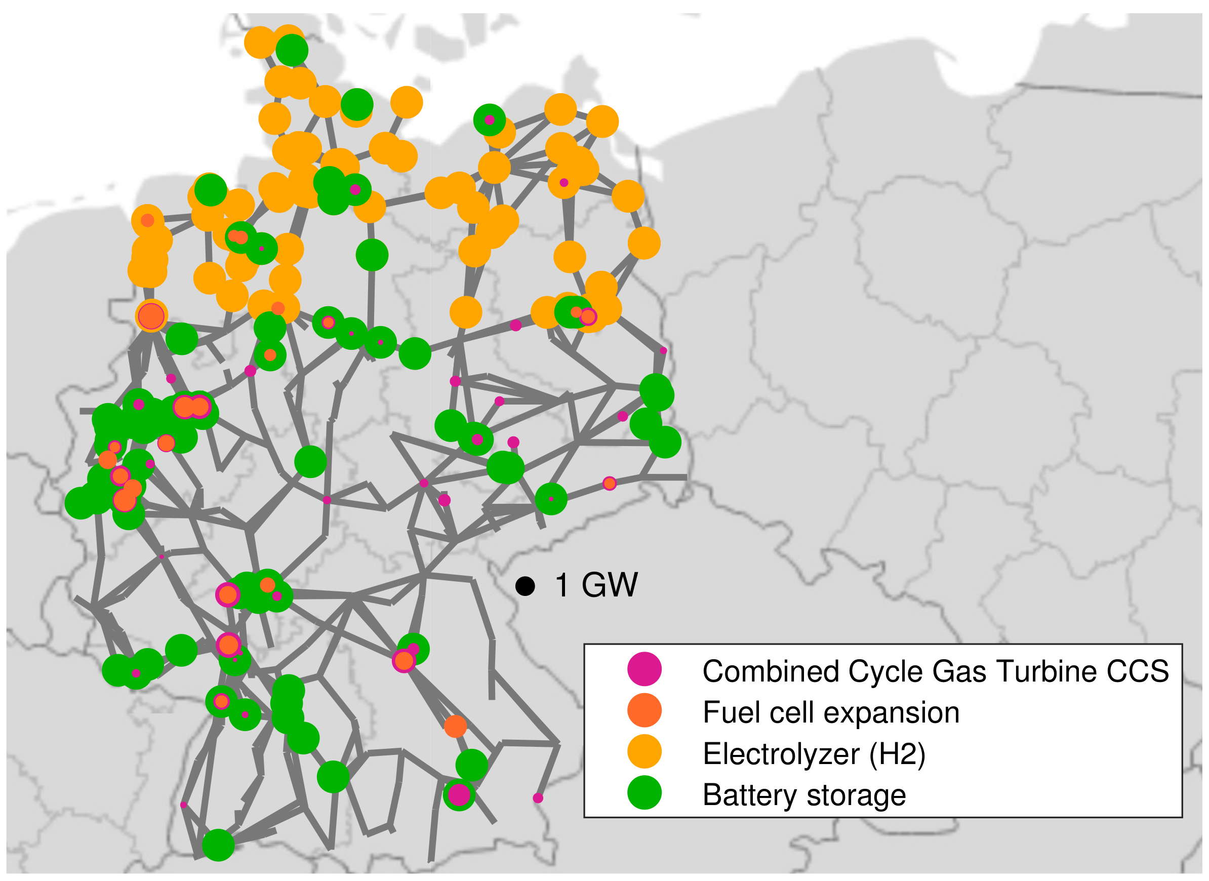
3.2. Expansion of Technologies Connected to the Power Transmission Grid
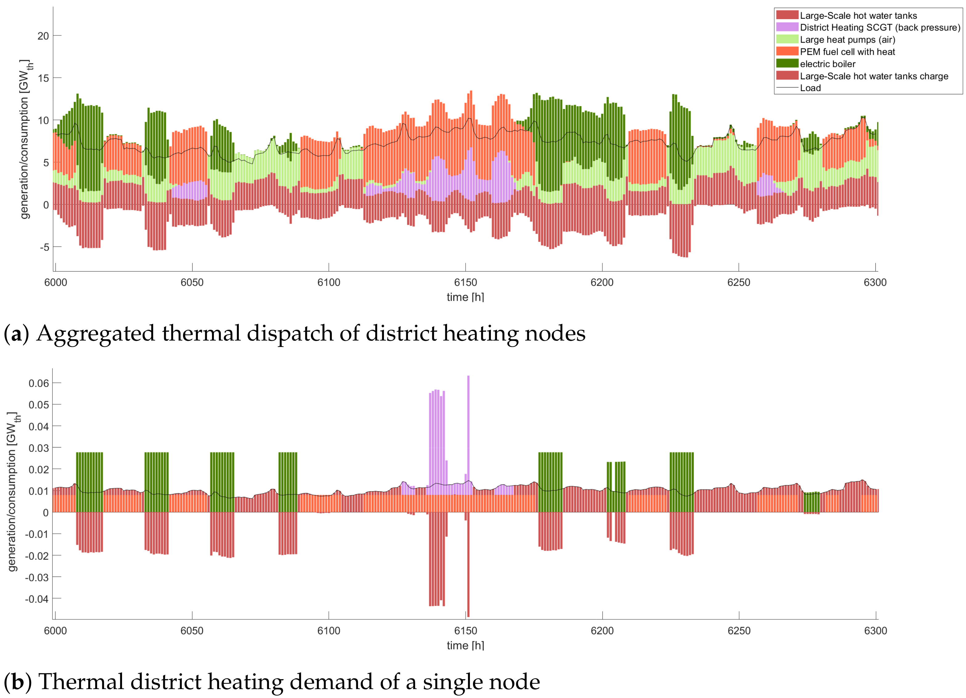
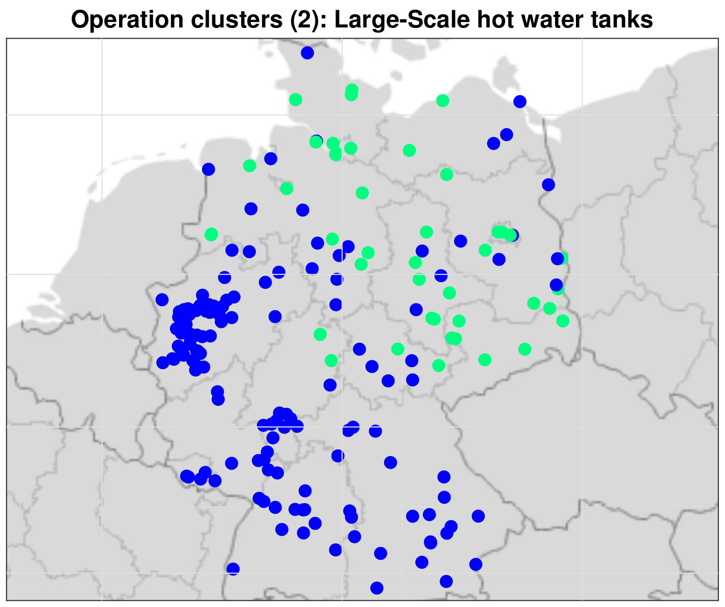
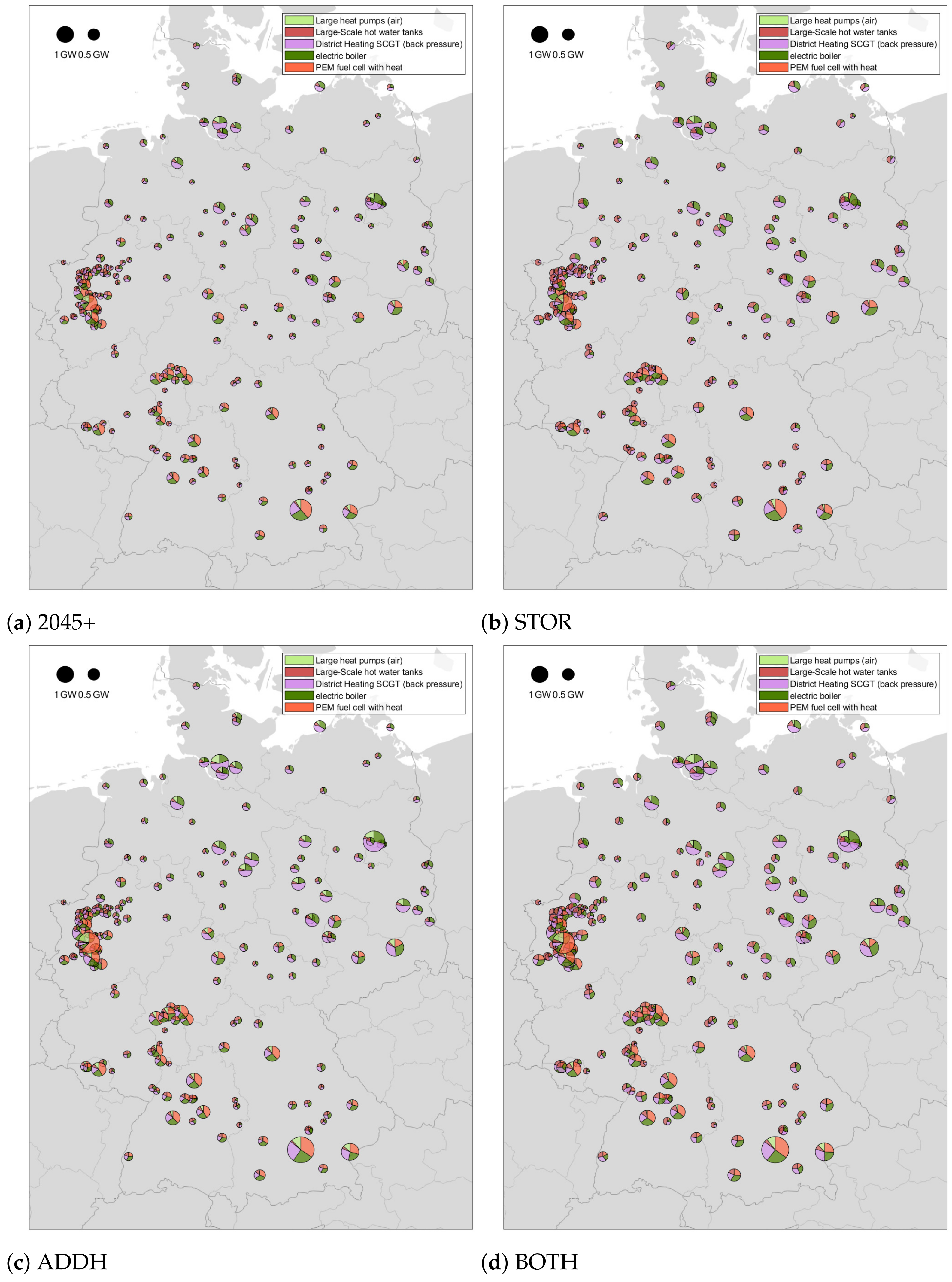
3.3. Expansion and Operation of District Heating Technologies
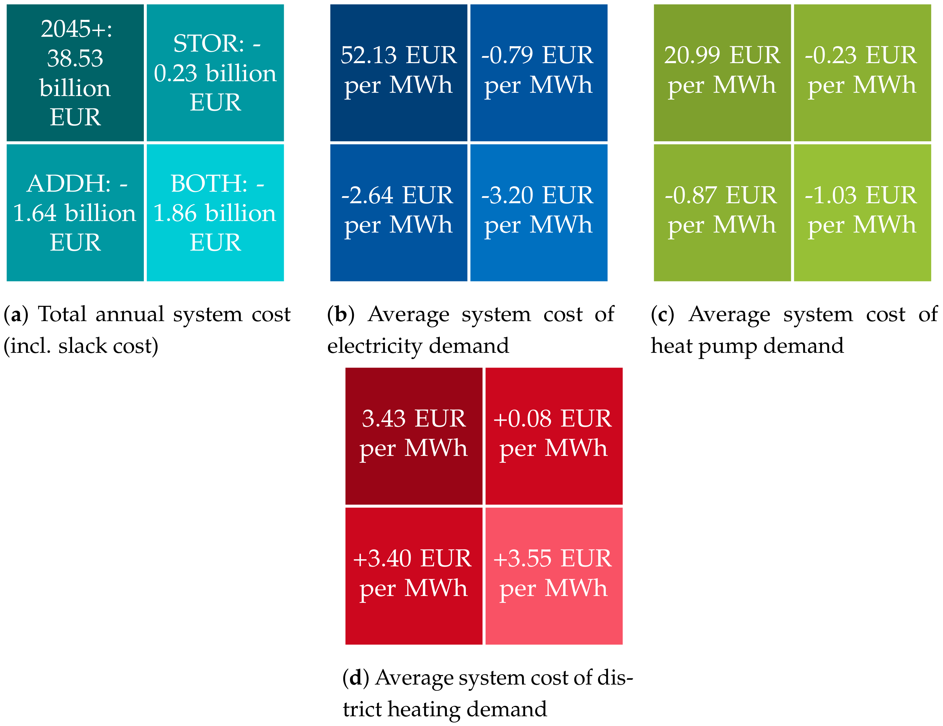
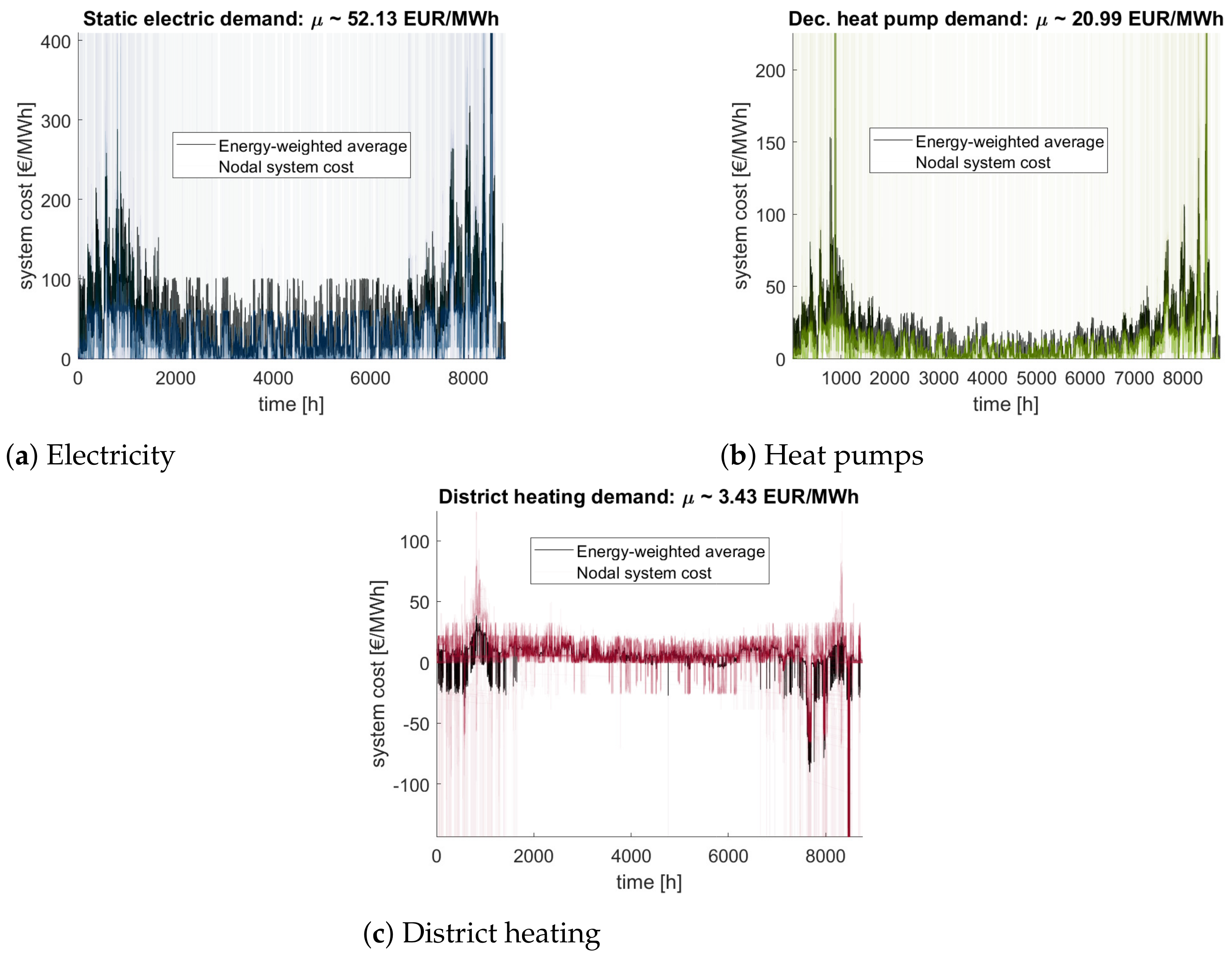
3.4. Quantifying Potential Benefits of District Heating
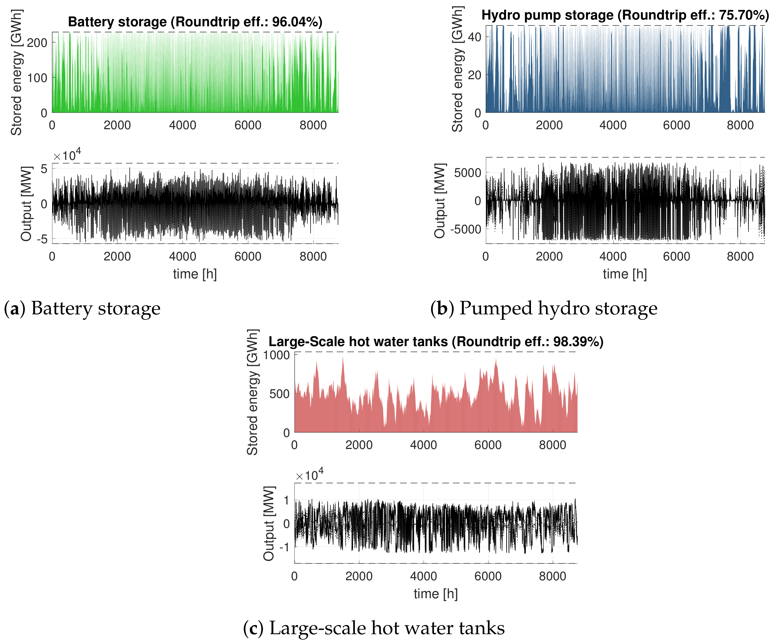
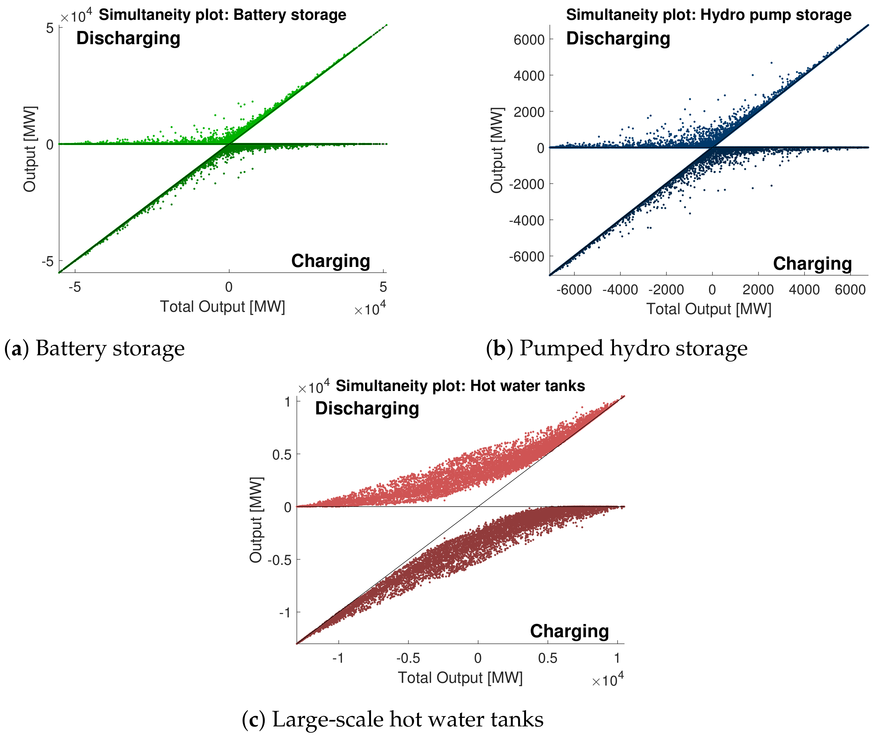
3.5. Comparison of Different Storage Operations
4. Discussion
- It does not make sense to model the cost of DHN expansion at the chosen model scale. First modeling attempts indicated that district heating is the preferred heating option and was always expanded to the maximum due to immense cost savings and increased flexibility—at least if expansion was allowed in sufficiently dense areas (compare Section 2.1.6). Apart from sensitivity studies, the informative value of model-endogenous DHN expansion is probably negligible without further knowledge.
- DH offers strong cost reduction and flexibility potential from the electric point of view. This does not yet take into account other effects, such as the integration of excess heat to reduce emissions.
- At least within the given sensitivities, the solution, apart from DH, changed only slightly. Although the total system cost is reduced, the rest of the energy system does not need to be specially adapted for this purpose. In other words: district heating can be integrated smoothly.
- Under the right circumstances, large-scale heat storage in district heating enables better RES integration which reduces cost and adds flexibility to the coupled electric system.
- Enhancing district heating networks (and thus implicitly their demand) simultaneously increases the potential of large-scale heat storage.
- At least within the parameter space of the sensitivity study, DHN expansion does not significantly reduce the need for high-voltage grid expansion and should rather be understood as an element to provide short-term flexibility.
Author Contributions
Funding
Acknowledgments
Conflicts of Interest
Abbreviations
| a | annum (per year) |
| CHP | Combined heat and power |
| CO2 | Carbon dioxide |
| CO2eq | Carbon dioxide equivalent |
| COP | Coefficient of performance |
| d | Day |
| el | Electric |
| DH | District heat(ing) |
| DHN | District heating network |
| G&TEP | Generation and transmission expansion |
| GHG | Greenhouse gas emissions |
| GW | Gigawatt |
| GWh | Gigawatt hour |
| HP | Heat pump |
| MW | Megawatt |
| MWh | Megawatt hour |
| RES | Renewable energy sources |
| RoR | Run-of-river |
| TES | Thermal energy storage |
| TW | Terrawatt |
| TWh | Terrawatthour |
| t | (metric) ton |
| th | thermal |
Appendix A. List of Used Parameters

| Heating Inputs | ||||
|---|---|---|---|---|
| Name | C | Capacity/Volume | Count | Parameters |
| Heat load DH | 86.5 TWh/145 TWh | 182 nodes | Section 2.2.7 [39] | |
| DH SCGT (backpressure) | [0 .. 84.5] GW | 182 | el: 0.5, : 1.0, CAPEX: 38.8k EUR/MW/a, OPEX (excl. fuel): 4 EUR/MWhel [3] | |
| DH water tanks | [0 .. 9] GWth/[0 .. 18] GWth | 182 | Section 2.2.7 [39], (dis)charge eff.: 100%, standing losses: 0.3 %/d, energy-to-power-ratio: 60.35, CAPEX: 972 EUR/MWth/a, OPEX: 0.1 EUR/MWhth, discharged [44], 0.5 tCO2/MW/a | |
| PEM fuel cell with heat | [0 .. 84.5] GW | 182 | el: 0.5, : 1.25, CAPEX: 120k EUR/MW/a [3], 6 tCO2/MW/a | |
| Large HP (air) | [0 .. 10.8] GWel | 182 | CAPEX: 32.4k EUR/MWel/a [3], OPEX (excl. el.): 1.7 EUR/MWh/el, Supply: 100 °C, Return: 50 °C, 10 tCO2/MWel/a | |
| Electric boiler | [0 .. Inf] | 182 | : 0.99, CAPEX: 3.9k EUR/MW/a, OPEX (excl. fuel): 0.4 EUR/MWhel [3], 2 tCO2/MW/a | |
| Heat load HP & Solar | 306.5 TWh/248 TWh | 508 nodes | Section 2.2.7 [39] | |
| Local HP | [0 .. Inf] | 508 | CAPEX: 101 EUR/kW/ael/a, 12.5 kgCO2/kW/a [67], Supply: 55 °C, Return: 25 °C | |
| Decentral water tanks | [0 .. Inf] | 508 | (dis)charge eff.: 100%, standing losses: 39%/d, energy-to-power-ratio: 0.15, CAPEX: 6.8 EUR/kW/ath/a, OPEX: 1.2 EUR/MWhth, discharged [67], 1 tCO2/MW/a | |
| Solarthermal | [0 .. 5.3] GWth | 508 | : 0.5, CAPEX: 29k EUR/MW/a [3], 1 tCO2/MW/a | |
| Heat load Gas | 8 TWh | 508 nodes | Section 2.2.7 [39] | |
| Gas boiler | [0 .. Inf] | 508 | : 1.0, CAPEX: 3.6k EUR/MW/a [67], 2 tCO2/MW/a | |
| Heat load Biomass | 54 TWh | 508 nodes | Section 2.2.7 [39] | |
| Biomass heating | [0 .. Inf] | 508 | : 0.9, CAPEX: 27k EUR/MW/a [67], 2 tCO2/MW/a | |
| Other Inputs | ||||
|---|---|---|---|---|
| Name | C | Capacity/Volume | Count | Parameters |
| Electric load | 720 TWh | 575 nodes | Section 2.2.7 [39] | |
| CCGT (gas) | 4538 MW | 16 | : 0.56, OPEX (excl. fuel): 4.4 EUR/MWh [3] | |
| SCGT (gas) | 145 MW | 3 | : 0.40, OPEX (excl. fuel): 4.4 EUR/MWh [3] | |
| STPP (gas) | 2027 MW | 34 | : 0.40, OPEX (excl. fuel): 4.4 EUR/MWh [3] | |
| ICE (gas) | 33 MW | 2 | : 0.44, OPEX (excl. fuel): 5.4 EUR/MWh [3] | |
| PP expansion (gas) | [0 .. 42] GW | 125 | : 0.48, CAPEX: 42.5k EUR/MW/a, OPEX (excl. fuel): 4.9 EUR/MWh, 4.8 tCO2/MW/a [3] | |
| CCGT CCS (gas) | [0 .. 25] GW | 50 | : 0.55, CAPEX: 34.8k EUR/MW/a, OPEX (excl. fuel): 75 EUR/MWh, 4 tCO2/MW/a | |
| Biomass PP (el.) | 6 GW [40] | 36 | : 0.375 | |
| Fuel cells (H2) | [0 .. 16] GW | 24 | : 0.5, CAPEX: 120k EUR/MW/a, 6 tCO2/MW/a | |
| Electrolyzer (H2) | [0 .. 366] GW | 122 | : 0.705, CAPEX: 28k EUR/MW/a, 4 tCO2/MW/a | |
| Onshore wind | [55 .. 401] GW | 418 | CAPEX: 38.4k EUR/MW/a [3], 11.2 tCO2/MW/a [47] | |
| Offshore wind | [7.8 .. 80] GW | 8 | CAPEX: 59.3k EUR/MW/a [3], 10.9 tCO2/MW/a [68] | |
| Photovoltaic | [54 .. 3138] GW | 477 | CAPEX: 15k EUR/MW/a, [3], 5 tCO2/MW/a [47] | |
| Run-of-river | 5.6 GW | 42 | 28 TWh [40], Locations [49] | |
| Hydro pump storage | 7.6 GW | 21 | Locations [49], energy-to-power-ratio: 6, roundtrip: 0.76 | |
| Battery storage | [0 .. 240] GW | 80 | CAPEX: 35k EUR/MW, OPEX: 1 EUR/MWhdischarge, roundtrip: 0.96, energy-to-power-ratio 4, (SDI E3-R135) [69], 5 tCO2/MW/a | |
| General Inputs | ||||
|---|---|---|---|---|
| Name | C | Capacity/Volume | Count | Parameters |
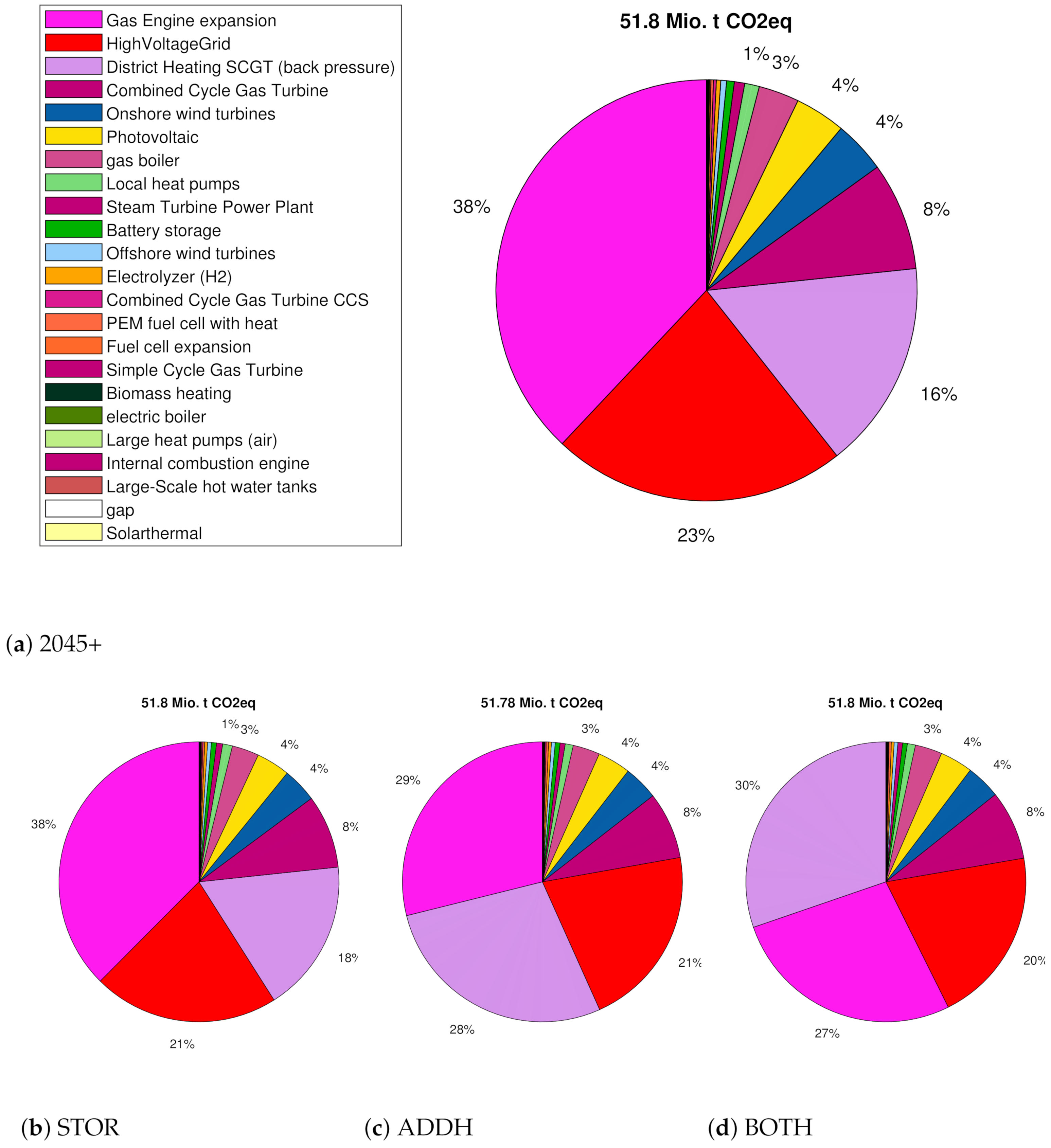
| CO2 | 1 | 51.8 Mio. t CO2eq (5% of Germany’s energy related emissions of 1990) | ||
| Natural gas | Inf | 1 | 26.30 EUR/MWhth [70], 0.2 kgCO2/MWhth | |
| Hydrogen (H2) | Inf | 1 | 51.29 EUR/MWhth, 0 kgCO2/MWhth | |
| Biomass | 193 TWh | 1 | 48.40 EUR/MWhth, 0 kgCO2/MWhth | |
| Transmission grid | 802 lines, 72 transformers | 575 nodes | New line: 88k EUR/km/a, 4 tCO2/km/a; Transformer: 1228 EUR/a/MW, 4 tCO2/MW/a (adapted from [33,71,72]) | |
Appendix B. Distribution of CO2 Emissions per Technology

Appendix C. District Heating Technology Expansion

References
- Werner, S. International review of district heating and cooling. Energy 2017, 137, 617–631. [Google Scholar] [CrossRef]
- David, A.; Mathiesen, B.V.; Averfalk, H.; Werner, S.; Lund, H. Heat Roadmap Europe: Large-Scale Electric Heat Pumps in District Heating Systems. Energies 2017, 10, 578. [Google Scholar] [CrossRef] [Green Version]
- Danish Energy Agency and Energinet. Technology Data: Generation of Electricity and District Heating; Danish Energy Agency and Energinet: Copenhagen, Denmark. Available online: https://ens.dk/sites/ens.dk/files/Statistik/technology_data_catalogue_for_el_and_dh_-_0009.pdf (accessed on 4 April 2021).
- Talebi, B.; Mirzaei, P.A.; Bastani, A.; Haghighat, F. A Review of District Heating Systems: Modeling and Optimization. Front. Built Environ. 2016, 2, 7839. [Google Scholar] [CrossRef] [Green Version]
- Wang, J.; You, S.; Zong, Y.; Cai, H.; Træholt, C.; Dong, Z.Y. Investigation of real-time flexibility of combined heat and power plants in district heating applications. Appl. Energy 2019, 237, 196–209. [Google Scholar] [CrossRef]
- Xu, X.; Lyu, Q.; Qadrdan, M.; Wu, J. Quantification of Flexibility of a District Heating System for the Power Grid. IEEE Trans. Sustain. Energy 2020, 11, 2617–2630. [Google Scholar] [CrossRef]
- Yifan, Z.; Wei, H.; Le, Z.; Yong, M.; Lei, C.; Zongxiang, L.; Ling, D. Power and energy flexibility of district heating system and its application in wide-area power and heat dispatch. Energy 2020, 190, 116426. [Google Scholar] [CrossRef]
- Kavviadas, K.; Jimenez Navarro, J.; Zucker, A.; Quoilin, S. Case Study on The Impact of Cogeneration and Thermal Storage on the Flexibility of the Power System; Publication Office of the European Commission: Petten, The Netherlands, 2018. [Google Scholar] [CrossRef]
- Lu, S.; Gu, W.; Zhou, J.; Zhang, X.; Wu, C. Coordinated dispatch of multi-energy system with district heating network: Modeling and solution strategy. Energy 2018, 152, 358–370. [Google Scholar] [CrossRef] [Green Version]
- Lund, H. Electric grid stability and the design of sustainable energy systems. Int. J. Sustain. Energy 2005, 24, 45–54. [Google Scholar] [CrossRef]
- Lund, H.; Möller, B.; Mathiesen, B.V.; Dyrelund, A. The role of district heating in future renewable energy systems. Energy 2010, 35, 1381–1390. [Google Scholar] [CrossRef]
- Gils, H.C. Balancing of Intermittent Renewable Power Generation by Demand Response and Thermal Energy Storage; Universität Stuttgart: Stuttgart, Germany, 2015. [Google Scholar] [CrossRef]
- Askeland, K.; Bozhkova, K.N.; Sorknæs, P. Balancing Europe: Can district heating affect the flexibility potential of Norwegian hydropower resources? Renew. Energy 2019, 141, 646–656. [Google Scholar] [CrossRef]
- Bernath, C.; Deac, G.; Sensfuß, F. Impact of sector coupling on the market value of renewable energies—A model-based scenario analysis. Appl. Energy 2021, 281, 115985. [Google Scholar] [CrossRef]
- Brown, T.; Schlachtberger, D.; Kies, A.; Schramm, S.; Greiner, M. Synergies of sector coupling and transmission reinforcement in a cost-optimised, highly renewable European energy system. Energy 2018, 160, 720–739. [Google Scholar] [CrossRef] [Green Version]
- Frysztacki, M.M.; Hörsch, J.; Hagenmeyer, V.; Brown, T. The strong effect of network resolution on electricity system models with high shares of wind and solar. Appl. Energy 2021, 291, 116726. [Google Scholar] [CrossRef]
- Neumann, F.; Brown, T. The near-optimal feasible space of a renewable power system model. Electr. Power Syst. Res. 2021, 190, 106690. [Google Scholar] [CrossRef]
- Müller, C.; Falke, T.; Hoffrichter, A.; Wyrwoll, L.; Schmitt, C.; Trageser, M.; Schnettler, A.; Metzger, M.; Huber, M.; Küppers, M.; et al. Integrated Planning and Evaluation of Multi-Modal Energy Systems for Decarbonization of Germany. Energy Procedia 2019, 158, 3482–3487. [Google Scholar] [CrossRef]
- Müller, C.; Hoffrichter, A.; Wyrwoll, L.; Schmitt, C.; Trageser, M.; Kulms, T.; Beulertz, D.; Metzger, M.; Duckheim, M.; Huber, M.; et al. Modeling framework for planning and operation of multi-modal energy systems in the case of Germany. Appl. Energy 2019, 250, 1132–1146. [Google Scholar] [CrossRef]
- Metzger, M.; Duckheim, M.; Franken, M.; Heger, H.J.; Huber, M.; Knittel, M.; Kolster, T.; Kueppers, M.; Meier, C.; Most, D.; et al. Pathways toward a Decarbonized Future—Impact on Security of Supply and System Stability in a Sustainable German Energy System. Energies 2021, 14, 560. [Google Scholar] [CrossRef]
- Li, Z.; Wu, W.; Wang, J.; Zhang, B.; Zheng, T. Transmission-Constrained Unit Commitment Considering Combined Electricity and District Heating Networks. IEEE Trans. Sustain. Energy 2016, 7, 480–492. [Google Scholar] [CrossRef]
- Schwaeppe, H.; Moser, A.; Paronuzzi, P.; Monaci, M. Generation and Transmission Expansion Planning with Respect to Global Warming Potential. In Proceedings of the 2021 IEEE Madrid PowerTech, Madrid, Spain, 28 June–2 July 2021; pp. 1–6. [Google Scholar] [CrossRef]
- Schwaeppe, H.; Böttcher, L.R.; Franken, M.S.; Schumann, K.; Monaci, M.; Punzo, A.; Paronuzzi, P. Mathematical Formulation of the Model: Deliverable 2.2; Version 1.0; IEEE, RWTH Aachen University: Aachen, Germany, 2020. [Google Scholar] [CrossRef]
- Rahmani, M.; Hug, G.; Kargarian, A. Comprehensive power transfer distribution factor model for large-scale transmission expansion planning. IET Gener. Transm. Distrib. 2016, 10, 2981–2989. [Google Scholar] [CrossRef]
- Horsch, J.; Brown, T. The role of spatial scale in joint optimisations of generation and transmission for European highly renewable scenarios. In Proceedings of the IEEE 2017 14th International Conference on the European Energy Market (EEM), Dresden, Germany, 6–9 June 2017; pp. 1–7. [Google Scholar] [CrossRef] [Green Version]
- Kavvadias, K.C.; Quoilin, S. Exploiting waste heat potential by long distance heat transmission: Design considerations and techno-economic assessment. Appl. Energy 2018, 216, 452–465. [Google Scholar] [CrossRef]
- Reinholdt, L.; Kristofferson, J.; Zühlsdorf, B.; Elmegaard, B.; Jensen, J.; Ommen, T.; Jørgensen, P.H. Heat Pump COP, Part 1: Generalized Method for Screening of System Integration Potentials. In Proceedings of the 13th IIR-Gustav Lorentzen Conference on Natural Refrigerants, Valencia, Spain, 18–20 June 2018; International Institute of Refrigeration: Paris, France, 2018; Volume 2, pp. 1097–1104. [Google Scholar] [CrossRef]
- Guelpa, E.; Verda, V. Thermal energy storage in district heating and cooling systems: A review. Appl. Energy 2019, 252, 113474. [Google Scholar] [CrossRef]
- Cao, K.K.; Von Krbek, K.; Wetzel, M.; Cebulla, F.; Schreck, S. Classification and Evaluation of Concepts for Improving the Performance of Applied Energy System Optimization Models. Energies 2019, 12, 4656. [Google Scholar] [CrossRef] [Green Version]
- Kiviluoma, J.; Meibom, P. Influence of wind power, plug-in electric vehicles, and heat storages on power system investments. Energy 2010, 35, 1244–1255. [Google Scholar] [CrossRef]
- Lythcke-Jørgensen, C.E.; Münster, M.; Ensinas, A.V.; Haglind, F. A method for aggregating external operating conditions in multi-generation system optimization models. Appl. Energy 2016, 166, 59–75. [Google Scholar] [CrossRef] [Green Version]
- Ketov, M. Marktsimulationen unter Berücksichtigung der Strom-Wärme-Sektorenkopplung [Market Simulations Considering Electricity-Heat-Sector Coupling. Ph.D. Thesis, RWTH Aachen and Print Production M. Wolff GmbH, Aachen, Germany, 2018. [Google Scholar]
- Barrios, H.; Roehder, A.; Natemeyer, H.; Schnettler, A. A benchmark case for network expansion methods. In Proceedings of the 2015 IEEE Eindhoven PowerTech, Eindhoven, The Netherlands, 29 June–2 July 2015; pp. 1–6. [Google Scholar] [CrossRef]
- Jalil-Vega, F.; Hawkes, A.D. The effect of spatial resolution on outcomes from energy systems modelling of heat decarbonisation. Energy 2018, 155, 339–350. [Google Scholar] [CrossRef]
- DDS Digital Data Services GmbH. PLZ8 GERMANY XXL: Infrastructure Data for Microregions. 2014. Available online: https://ddsgeo.de/daten/datenpakete/plz8-deutschland-xxl (accessed on 20 May 2021).
- Dochev, I.; Peters, I.; Seller, H.; Schuchardt, G.K. Analysing district heating potential with linear heat density. A case study from Hamburg. Energy Procedia 2018, 149, 410–419. [Google Scholar] [CrossRef]
- Möller, B.; Werner, S. Quantifying the Potential for District Heating and Cooling in EU Member States: Deliverable No. D 2.2: Public Document; University of Flensburg: Flensburg, Germany, 2016; Available online: https://heatroadmap.eu/wp-content/uploads/2018/09/STRATEGO-WP2-Background-Report-6-Mapping-Potenital-for-DHC.pdf (accessed on 26 October 2021).
- Chicherin, S.; Mašatin, V.; Siirde, A.; Volkova, A. Method for Assessing Heat Loss in A District Heating Network with A Focus on the State of Insulation and Actual Demand for Useful Energy. Energies 2020, 13, 4505. [Google Scholar] [CrossRef]
- Prognos, Öko-Institut, Wuppertal-Institut. Klimaneutrales Deutschland 2045: Wie Deutschland Seine Klimaziele Schon vor 2050 Erreichen Kann: Langfassung im Auftrag von Stiftung Klimaneutralität, Agora Energiewende und Agora Verkehrswende [Towards a Climate-Neutral Germany by 2045: How Germany Can Reach Its Climate Targets before 2050: Long Version Commissioned by the Stiftung Klimaneutralität, Agora Energiewende and Agora Verkehrswende]. Executive Summary Available in English. Available online: https://www.agora-energiewende.de/en/publications/towards-a-climate-neutral-germany-2045-executive-summary/ (accessed on 16 November 2021).
- Bundesnetzagentur für Elektrizität, Gas, Telekommunikation, Post und Eisenbahnen. Bedarfsermittlung 2021–2035: Bestätigung Netzentwicklungsplan Strom [Assessment of Needs 2021–2035: Confirmation of Grid Development Plan Electricity]. 2022. Available online: https://www.netzentwicklungsplan.de/de/netzentwicklungsplaene/netzentwicklungsplan-2035-2021 (accessed on 30 January 2022).
- Thie, N.; Franken, M.; Schwaeppe, H.; Bottcher, L.; Muller, C.; Moser, A.; Schumann, K.; Vigo, D.; Monaci, M.; Paronuzzi, P.; et al. Requirements for Integrated Planning of Multi-Energy Systems. In Proceedings of the 2020 6th IEEE International Energy Conference (ENERGYCon), Gammarth, Tunis, Tunisia, 28 September–1 October 2020; pp. 696–701. [Google Scholar] [CrossRef]
- Schumann, K.; Schwaeppe, H.; Böttcher, L.R.; Franken, M.S.; Thie, N.; Bischi, A.; Gordini, A.; Ferrari, L.; Taştan, İ.; Monaci, M. Definition of Common Scenario Framework, Data/Modelling Requirements and Use Cases: Deliverable 2.1; Version 2.0; RWTH Aachen University: Aachen, Germany, 2020. [Google Scholar] [CrossRef]
- Schumann, K.; Schwaeppe, H.; Böttcher, L.R.; Hein, L.; Hälsig, P. Description of Workflow Coordination: Deliverable 3.1; Version 1.0. Available online: https://publications.rwth-aachen.de/record/834498 (accessed on 26 November 2021). [CrossRef]
- Danish Energy Agency and Energinet. Technology Data: Energy Storage. Available online: https://ens.dk/en/our-services/projections-and-models/technology-data (accessed on 26 November 2021).
- Weisser, D. A guide to life-cycle greenhouse gas (GHG) emissions from electric supply technologies. Energy 2007, 32, 1543–1559. [Google Scholar] [CrossRef]
- Kaldellis, J.K.; Apostolou, D. Life cycle energy and carbon footprint of offshore wind energy. Comparison with onshore counterpart. Renew. Energy 2017, 108, 72–84. [Google Scholar] [CrossRef]
- Pehl, M.; Arvesen, A.; Humpenöder, F.; Popp, A.; Hertwich, E.G.; Luderer, G. Understanding future emissions from low-carbon power systems by integration of life-cycle assessment and integrated energy modelling. Nat. Energy 2017, 2, 939–945. [Google Scholar] [CrossRef]
- Krishnan, R.; Nair, K.R.M. Carbon Footprint of Transformer and the Potential for Reduction of CO2 Emissions. In Proceedings of the 2019 IEEE 4th International Conference on Technology, Informatics, Management, Engineering & Environment (TIME-E), Bali, Indonesia, 13–15 November 2019; pp. 138–143. [Google Scholar] [CrossRef]
- Weibezahn, J.; Weinhold, R.; Gerbaulet, C.; Kunz, F. Open Power System Data. 2020. Data Package Conventional Power Plants. Version 2020-10-01. (Primary Data from Various Sources, for a Complete List See URL). Available online: https://data.open-power-system-data.org/conventional_power_plants/ (accessed on 26 November 2021). [CrossRef]
- Hersbach, H.; Bell, B.; Berrisford, P.; Biavati, G.; Horányi, A.; Muñoz Sabater, J.; Nicolas, J.; Peubey, C.; Radu, R.; Rozum, I.; et al. ERA5 Hourly Data on Single Levels from 1979 to Present. 2018. Available online: https://cds.climate.copernicus.eu/cdsapp#!/dataset/reanalysis-era5-single-levels?tab=overview (accessed on 26 October 2021). [CrossRef]
- Uwe, K.; Guido, P.; Stephan, G.; Birgit, S.; Stephen, B.; Cord, K. Feedinlib (Oemof)—Creating Feed-in Time Series—v0.0.12. 2019. Available online: https://zenodo.org/record/2554102#.YjmjITURU2w (accessed on 26 November 2021). [CrossRef]
- Sabine, H.; Uwe, K.; Birgit, S.; Stickler, B.; Kyri, P.; Velibor, Z.; Kumar, S. Wind-Python/Windpowerlib: Silent Improvements. 2021. Available online: https://zenodo.org/record/4591809#.YjmjMDURU2w (accessed on 26 November 2021). [CrossRef]
- Raths, S. International ETG Congress 2015: Die Energiewende—Blueprints for the New Energy Age; IEEE: Piscataway, NJ, USA, 2015. [Google Scholar]
- Cramer, W.; Schumann, K.; Andres, M.; Vertgewall, C.; Monti, A.; Schreck, S.; Metzger, M.; Jessenberger, S.; Klaus, J.; Brunner, C.; et al. A simulative framework for a multi-regional assessment of local energy markets—A case of large-scale electric vehicle deployment in Germany. Appl. Energy 2021, 299, 117249. [Google Scholar] [CrossRef]
- Federal Office of Statistics Germany. Living and Working in Germany–Microcensus; Statistische Bundesamt: Wiesbaden, Germany, 2016.
- Fraunhofer ISI. Energieverbrauch des Sektors Gewerbe, Handel, Dienstleistungen (GHD) in Deutschland für die Jahre 2011 bis 2013 [Energy Consumption of the Trade, Commerce and Services Sector in Germany for the Years 2011 to 2013]; Fraunhofer Institute for Systems and Innovation Research ISI: Karlsruhe, Germany; München, Germany; Nürnberg, Germany, 2015. [Google Scholar]
- Loga, T.; Stein, B.; Diefenbach, N. TABULA building typologies in 20 European countries—Making energy-related features of residential building stocks comparable. Energy Build. 2016, 132, 4–12. [Google Scholar] [CrossRef]
- Falke, T.; Krengel, S.; Meinerzhagen, A.K.; Schnettler, A. Multi-objective optimization and simulation model for the design of distributed energy systems. Appl. Energy 2016, 184, 1508–1516. [Google Scholar] [CrossRef]
- Smolka, T.; Dederichs, T.; Gödde, M.; Schnettler, A. Potentiale und Rahmenbedinungen für Einen Flächendeckenden Einsatz von Smart Metering für Stadtwerke [Potentials and Conditions for the Widespread Use of Smart Metering for Municipal Utilities]. ETG-Fachbericht, Band 130. 2011. Available online: https://www.vde-verlag.de/proceedings-en/453376050.html (accessed on 11 October 2021).
- VDEW. Repräsentative VDEW-Lastprofile [Representative VDEW Load Profiles]. VDEW Mater., M-32. 1999. Available online: https://www.bdew.de/media/documents/1999_Repraesentative-VDEW-Lastprofile.pdf (accessed on 11 November 2021).
- BDEW Bundesverband der Energie- und Wasserwirtschaft e.V. Abwicklung von Standardlastprofilen Gas: BDEW/VKU/GEODE-Leitfaden [Processing of Standard Load Profiles Gas: BDEW/VKU/GEODE Guideline]. 2014. Available online: https://www.gvp-netz.de/fileadmin/Dateien/dokumente/14-06-30_KOV_VII_LF_Abwicklung_von_SLP_Gas.pdf (accessed on 11 November 2021).
- Fraunhofer IWES. Interaktion EE-Strom, Wärme und Verkehr: Endbericht; Fraunhofer-Institut für Windenergie und Energiesystemtechnik: Kassel, Germany, 2015; Available online: https://www.iee.fraunhofer.de/content/dam/iee/energiesystemtechnik/de/Dokumente/Veroeffentlichungen/2015/Interaktion_EEStrom_Waerme_Verkehr_Endbericht.pdf (accessed on 26 November 2021).
- Konstantin, P. Praxisbuch der FernwäRmeversorgung: Systeme, Netzaufbauvarianten, Kraft-Wärme-Kopplung, Kostenstrukturen und Preisbildung [Practice Book on District Heating Supply: Systems, Network Design Variants, Cogeneration, Cost Structures and Pricing], 1. Aufl. 2018 ed.; Springer: Berlin/Heidelberg, Germany, 2018. [Google Scholar]
- Trutnevyte, E. Does cost optimization approximate the real-world energy transition? Energy 2016, 106, 182–193. [Google Scholar] [CrossRef]
- Hawker, G.S.; Bell, K.R.W. Making energy system models useful: Good practice in the modelling of multiple vectors. WIREs Energy Environ. 2020, 9, 347. [Google Scholar] [CrossRef]
- Lund, H.; Østergaard, P.A.; Nielsen, T.B.; Werner, S.; Thorsen, J.E.; Gudmundsson, O.; Arabkoohsar, A.; Mathiesen, B.V. Perspectives on fourth and fifth generation district heating. Energy 2021, 227, 120520. [Google Scholar] [CrossRef]
- Danish Energy Agency and Energinet. Technology Data. Heating installations. In Technology Descriptions and Projections for Long-Term Energy System Planning: Individual Heating; Danish Energy Agency: Copenhagen, Denmark, 2021. Available online: https://ens.dk/sites/ens.dk/files/Analyser/technology_data_catalogue_for_individual_heating_installations.pdf (accessed on 12 March 2022).
- Arvesen, A.; Nes, R.N.; Huertas-Hernando, D.; Hertwich, E.G. Life cycle assessment of an offshore grid interconnecting wind farms and customers across the North Sea. Int. J. Life Cycle Assess. 2014, 19, 826–837. [Google Scholar] [CrossRef] [Green Version]
- Danish Energy Agency and Energinet. Technology Data. In Energy Storage: Technology Descriptions and Projections for Long-Term Energy System Planning; Danish Energy Agency: Copenhagen, Denmark, 2018. Available online: https://ens.dk/sites/ens.dk/files/Analyser/technology_data_catalogue_for_energy_storage.pdf (accessed on 12 March 2022).
- Bundesnetzagentur für Elektrizität, Gas, Telekommunikation, Post und Eisenbahnen. Genehmigung des Szenariorahmens 2021–2035 [Approval of the 2021–2035 Scenario Framework]. 2020. Available online: https://www.netzentwicklungsplan.de/sites/default/files/paragraphs-files/Szenariorahmen_2035_Genehmigung_1.pdf (accessed on 30 January 2022).
- Harrison, G.P.; Maclean, E.J.; Karamanlis, S.; Ochoa, L.F. Life cycle assessment of the transmission network in Great Britain. Energy Policy 2010, 38, 3622–3631. [Google Scholar] [CrossRef] [Green Version]
- Wei, W.; Wu, X.; Li, J.; Jiang, X.; Zhang, P.; Zhou, S.; Zhu, H.; Liu, H.; Chen, H.; Guo, J.; et al. Ultra-high voltage network induced energy cost and carbon emissions. J. Clean. Prod. 2018, 178, 276–292. [Google Scholar] [CrossRef]


| Large-Scale Hot Water Tanks | Pit Thermal Energy Storage | Lithium-ion NMC Battery (Ulitity-scale) | |
|---|---|---|---|
| Energy capacity | 175 MWhth | 4500 MWhth | 8 MWhel |
| Cost (EUR/MWh) | 3000 | 470 | 255,000 |
| Roundtrip Efficiency | 0.98 | 0.70 | 0.92 |
Publisher’s Note: MDPI stays neutral with regard to jurisdictional claims in published maps and institutional affiliations. |
© 2022 by the authors. Licensee MDPI, Basel, Switzerland. This article is an open access article distributed under the terms and conditions of the Creative Commons Attribution (CC BY) license (https://creativecommons.org/licenses/by/4.0/).
Share and Cite
Schwaeppe, H.; Böttcher, L.; Schumann, K.; Hein, L.; Hälsig, P.; Thams, S.; Baquero Lozano, P.; Moser, A. Analyzing Intersectoral Benefits of District Heating in an Integrated Generation and Transmission Expansion Planning Model. Energies 2022, 15, 2314. https://doi.org/10.3390/en15072314
Schwaeppe H, Böttcher L, Schumann K, Hein L, Hälsig P, Thams S, Baquero Lozano P, Moser A. Analyzing Intersectoral Benefits of District Heating in an Integrated Generation and Transmission Expansion Planning Model. Energies. 2022; 15(7):2314. https://doi.org/10.3390/en15072314
Chicago/Turabian StyleSchwaeppe, Henrik, Luis Böttcher, Klemens Schumann, Lukas Hein, Philipp Hälsig, Simon Thams, Paula Baquero Lozano, and Albert Moser. 2022. "Analyzing Intersectoral Benefits of District Heating in an Integrated Generation and Transmission Expansion Planning Model" Energies 15, no. 7: 2314. https://doi.org/10.3390/en15072314