
Machine Learning-Enhanced Play Fairway Analysis for Uncertainty Characterization and Decision Support in Geothermal Exploration


Earth Resources Laboratory, Massachusetts Institute of Technology, Cambridge, MA 02139, USA
*
Author to whom correspondence should be addressed.
†
Current address: Chevron Technical Center, Houston, TX 77002, USA.
Energies 2022, 15(5), 1929; https://doi.org/10.3390/en15051929
Submission received: 4 January 2022
/
Revised: 18 February 2022
/
Accepted: 28 February 2022
/
Published: 7 March 2022
(This article belongs to the Special Issue Machine Learning Applications in Petroleum Industries and Geothermal Systems)
Abstract
:Geothermal exploration has traditionally relied on geological, geochemical, or geophysical surveys for evidence of adequate enthalpy, fluids, and permeability in the subsurface prior to drilling. The recent adoption of play fairway analysis (PFA), a method used in oil and gas exploration, has progressed to include machine learning (ML) for predicting geothermal drill site favorability. This study introduces a novel approach that extends ML PFA predictions with uncertainty characterization. Four ML algorithms—logistic regression, a decision tree, a gradient-boosted forest, and a neural network—are used to evaluate the subsurface enthalpy resource potential for conventional or EGS prospecting. Normalized Shannon entropy is calculated to assess three spatially variable sources of uncertainty in the analysis: model representation, model parameterization, and feature interpolation. When applied to southwest New Mexico, this approach reveals consistent enthalpy trends embedded in a high-dimensional feature set and detected by multiple algorithms. The uncertainty analysis highlights spatial regions where ML models disagree, highly parameterized models are poorly constrained, and predictions show sensitivity to errors in important features. Rapid insights from this analysis enable exploration teams to optimize allocation decisions of limited financial and human resources during the early stages of a geothermal exploration campaign.
1. Introduction
The identification of geothermal sites has historically depended on field evidence of hot fluids circulating at depth, including the presence of geysers, fumaroles, mud pots, and diagnostic mineral deposits [1]. However, surface manifestations such as these are absent for blind geothermal systems, which require more advanced methods for discovery. With the support of the United States Department of Energy, researchers recently pivoted to play fairway analysis (PFA) as a method adopted from the oil and gas industry for regional exploration opportunity identification and risk assessments [2]. Conceptually, PFA decomposes risk into the constituent elements of a successful play, e.g., reservoir, source, seal, and trap geometry for hydrocarbons [3]. Maps are generated for each risk element based on available data, including published research, field observations, and modeling results. Taking the collective evidence as input, subject matter experts define a chance of success for each element and then use statistical approaches to combine multiple risk element maps into a single view of play favorability [4]. Geothermal PFA studies typically divide the geothermal system into enthalpy (heat), permeability, and fluids risk elements, which are then combined by weighted average based on data confidence or expert opinion [5,6,7]. The resulting maps reveal geothermal fairways inclusive of both surface-visible and blind geothermal systems.
Following the ongoing trend of digital transformation in the earth sciences [8], both unsupervised and supervised machine learning techniques are now being incorporated into geothermal exploration workflows. Unsupervised methods learn directly from the structure of geologic, geochemical, geophysical, and other relevant data sets. One such approach applies dimensionality-reduction techniques such as principal component analysis or non-negative matrix factorization to consolidate meaningful signals within the input data sets (or “features”), producing a smaller number of derived features useful for identifying data clusters [9,10,11]. However, the physical significance of these clusters is not unequivocally clear. Alternatively, supervised algorithms require labeled example data for training before providing predictive values. When applied to field data, advanced supervised methods such as artificial neural networks (ANN) have shown promise in predicting geothermal favorability [12]. Still, selecting which supervised algorithm to use for prediction either relies on an a priori decision or competitive ranking of several algorithms by some metric of predictive success [13,14]. This study considers how the combined insights from more than one model can define both robust trends and areas of disagreement, thereby revealing a relative measure of uncertainty in the prediction system.
Uncertainty derives from many sources in subsurface resource exploration, be it for water, hydrocarbons, minerals, or enthalpy [15]. To build an integrated understanding of the spatial variation in earth properties, data spanning multiple scales and sensitivities must be combined, including detailed point samples, well log records, and coarser potential field measurements [13]. The decisions made as these data are incorporated into models become important sources of uncertainty that have downstream impacts on prospect selection, appraisal, and development choices made by a firm. The following sections introduce a novel methodology that extends the use of ML for PFA predictions to also incorporate uncertainty estimation with normalized Shannon entropy as the uncertainty metric. Specifically, this study characterizes three varieties of uncertainty: those associated with the choice of machine learning model architecture; those in the learned parameters within a single model; and those in the input feature data and their preparation. This approach is applied to a region of New Mexico with known geothermal resource areas (KGRAs) to illustrate how the methodology provides comprehensive predictions of resource presence, unique insights on prediction confidence, and the opportunity for data-driven early-stage resource allocations and decision making in geothermal projects.
2. Materials and Methods
2.1. Data Sources
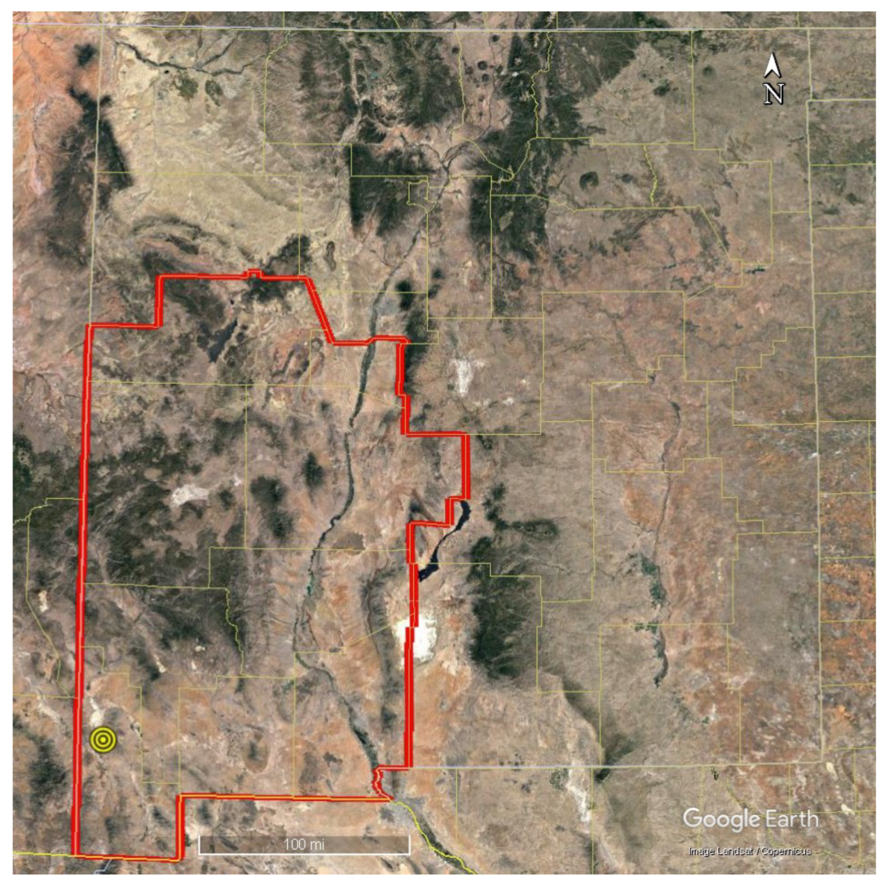
This investigation brings together twenty-five (25) public sets of data, hereafter referred to as “features,” that spatially cover a 37,600 square mile area of interest (AOI) in southwest New Mexico (Figure 1). The original feature data format varied between pre-gridded raster files, point sets with overlapping measurements, non-overlapping point sets, and line data. Fourteen features were retrieved from the Geothermal Data Repository archival submission for a PFA led by the Los Alamos National Lab [16,17]. Additional features were collected from published works, open-access databases, or derived from the original sources as secondary products. Table 1 lists the features by measurement, original format, and the source reference where appropriate. One or more exploration risk elements are associated with each feature based on their known sensitivities: fluids (F), heat (H), and/or permeability (P). These assignments help illustrate the variety and breadth of features included in the study, but they play no role in the ML PFA workflow to avoid introducing cognitive bias on the final results.
The models developed here remain agnostic on the specific geothermal system that a firm might intend on developing within the area being explored. In particular, we focus solely on the enthalpy risk element, since it uniquely contributes to favorability across hydrothermal, advanced closed loop (ACL), and enhanced geothermal systems (EGS). For hydrothermal, separate modeling of subsurface permeability and fluids favorability could follow the same methodology but would necessarily require different response variables for the prediction.
Well data within the study area are available from the Southern Methodist University (SMU) Heat Flow Database, which was accessed via the SMU node of the National Geothermal Data System [31]. Heat-flow values in the database derive from geothermal-gradient and thermal-conductivity values published in journal articles, books, official reports, and other sources [32]. Geothermal gradients are defined from direct downhole wireline readings or approximated based on corrected bottom-hole temperatures [33]. By contrast, thermal conductivity values rely on average regional stratigraphy, which introduces uncertainty associated with underrepresented subsurface heterogeneity [14]. Rather than incorporate thermal conductivity estimation as an additional source of uncertainty in this study, the geothermal gradient was selected over heat flow as the response variable and proxy for heat presence. The final collection of ground-truth geothermal gradient values amount to 599 measurements focused primarily on the shallow subsurface since over 80% of the wells do not exceed 500 m in depth (Figure A26).
2.2. Data Conditioning Workflow
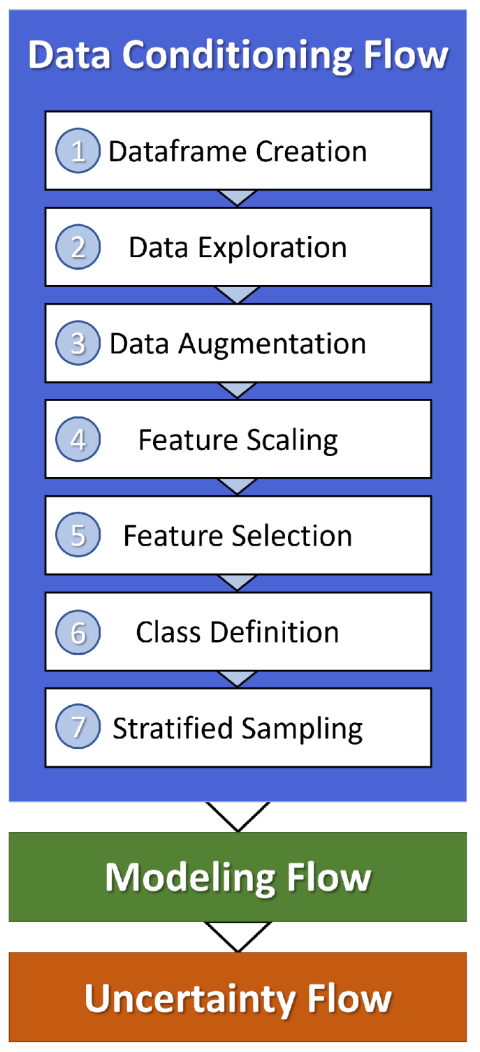
Before the collected data sets could be analyzed using ML methods, they were converted to complete GIS rasters as illustrated in Figure A1, Figure A2, Figure A3, Figure A4, Figure A5, Figure A6, Figure A7, Figure A8, Figure A9, Figure A10, Figure A11, Figure A12, Figure A13, Figure A14, Figure A15, Figure A16, Figure A17, Figure A18, Figure A19, Figure A20, Figure A21, Figure A22, Figure A23, Figure A24 and Figure A25. Figure 2 describes the data-conditioning workflow required to further prepare the data for modeling. The rasters were merged into a single matrix, where each column contains the set of values for a single feature, and the 15,007 rows define a spatial grid within the AOI polygon.
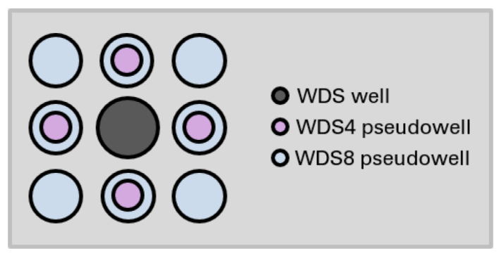
Given that the AOI spans over 97,000 km, the sparse observations in the SMU well data set (WDS) could be problematic for a supervised ML approach. Data augmentation and imputation methods serve to increase the size and completeness of data sets using simplifying assumptions, heuristics, or even complex modeling [35]. Here, we utilize the heuristic at the heart of variography, which relies on the increase in auto-correlation as the spatial distance decreases for geographic-related data sets [36]. Specifically, we created a larger data set (WDS4) by placing an additional four points to the north, south, east, and west of each WDS well location using 0.01 offsets to the well’s geographic coordinates (Figure 3). Geothermal-gradient values were determined by applying kriging to WDS, and feature values were extracted directly from the feature GIS layers at these “pseudowell” locations (Figure A27). Extending this method further, another augmented data set (WDS8) placed additional pseudowells to the NE, SE, NW, and SW, resulting in eight pseudowells for every original well in WDS (Figure 3). By keeping the pseudowell step-out distance smaller than the grid interval used throughout the study, the spatial correlation length scale imposed by augmentation remains below the resolution of the prediction models and thus should not overly influence the results. This workflow resulted in an expansion of the WDS data to 2995 and 5386 observations for WDS4 and WDS8, respectively. The ML methods described in Section 2.3 were applied to all three data sets in order to observe how the augmentation strategy impacted the results.
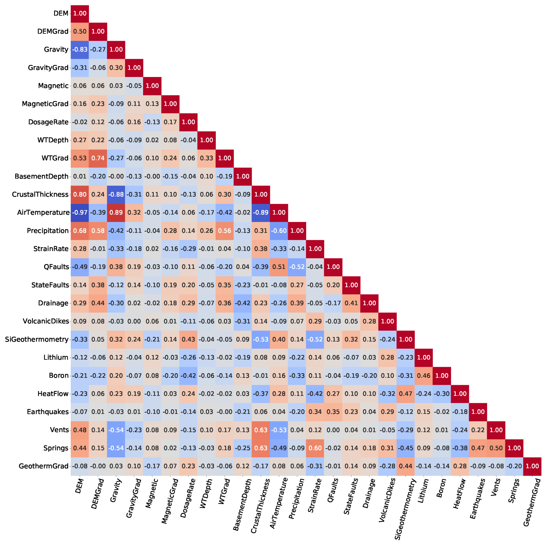
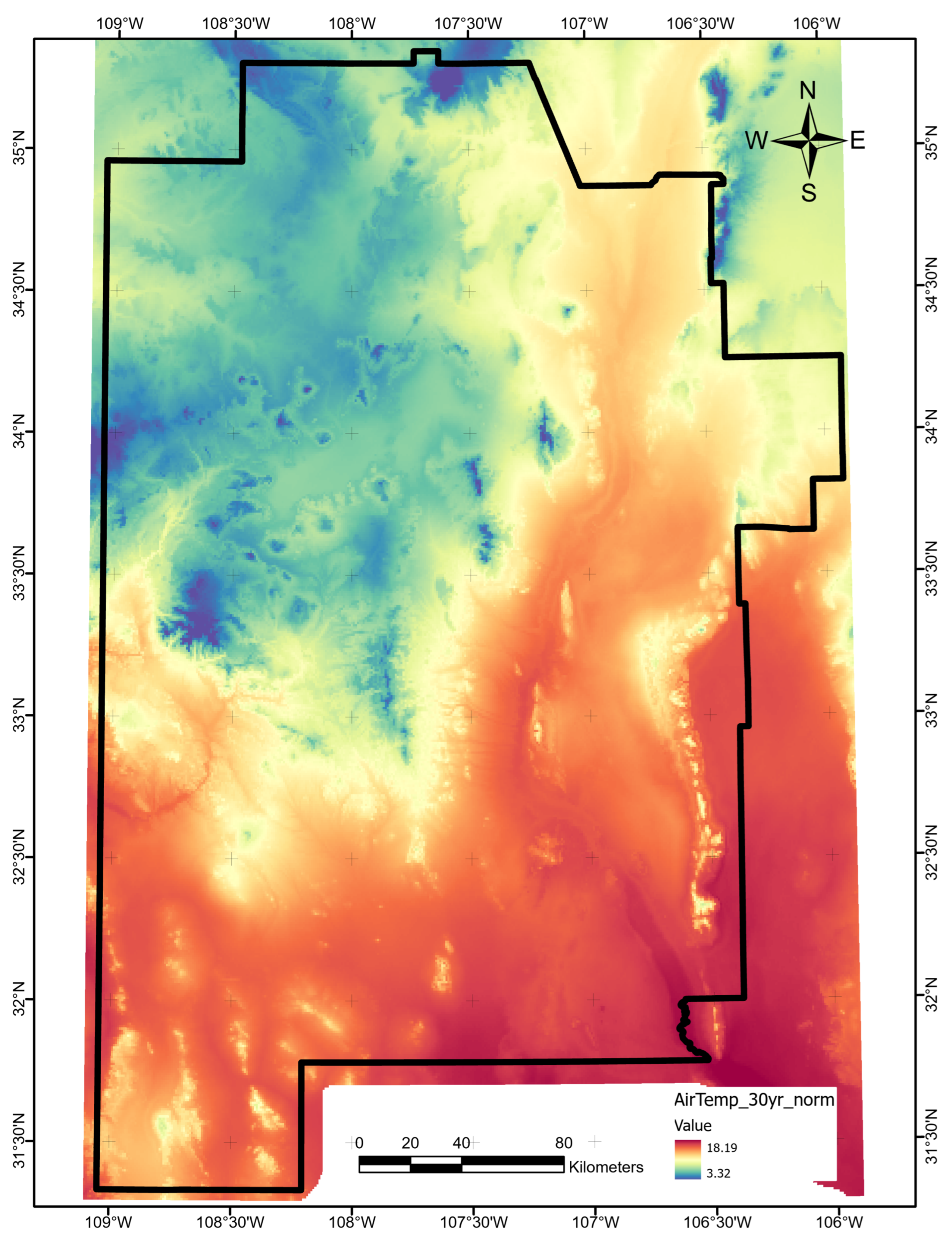
In the next series of conditioning workflow steps, feature data distributions were updated before modeling. Large differences in the average value and range of each feature can adversely impact some ML algorithms, so all features were standardized to zero mean and unit variance. Additionally, the data were reshaped by the Yeo–Johnson method, which uses a one-parameter family of transformations to replace distribution skewness with more Gaussian-like symmetry as required by some statistical methods [37]. Figure 4 illustrates pairwise correlation calculations between each of the features listed in Table 1, after rescaling and reshaping. Large correlation coefficients highlight relationships violating the assumption of feature linear independence. Average air temperature stands out as highly collinear with multiple variables: DEM (correlation ), gravity anomaly (), and crustal thickness (). The correlation value between air temperature and DEM is consistent with the fact that PRISM air temperatures are derived from a climatic regression with DEM as an input [38]. Given the near-interchangeability in the value of information both provide for prediction, we chose to remove average air temperature to simplify the input data and ML models.
The response variable, geothermal gradient, can be treated as a continuous variable and predicted directly using regression methods. Alternatively, binning geothermal gradient into discrete ranges changes the approach into a classification problem. Classification maps have a direct corollary to the classic green–yellow–red categorical PFA favorability maps, lithology-segmented geologic maps, and other displays of complex geospatial information. We also prefer the more conservative aspect of discrete class prediction. By contrast, regression provides seemingly precise estimates that could be mistaken for certain in a very under-constrained problem. Table 2 outlines the gradient ranges and associated class labels adopted for this study.
Additional preparation of data sets WDS, WDS4, and WDS8 included removing records with undefined values or rare negative geothermal gradients, amounting to a 0.5% reduction in data count. The remaining records were labeled using the classification scheme in Table 2. Class value distributions for the well data sets are shown in Table 3. Note that class imbalance exists in all three data sets; higher-grade (class 2 or 3) geothermal gradient examples dominate, with many fewer non-thermal (class 0) examples. Managing class imbalance is an area of active research, particularly for cases such as this where under-representation of the minority class makes common rebalancing algorithms ineffective [40]. As additional techniques become recommended, managing class imbalance should become a fundamental step in the conditioning workflow described in Figure 2.
Supervised ML methods learn from the data supplied during the training step of model building. However, over-training can lead to high model variance, where the in-sample predictive power observed with training data does not generalize to out-of-sample data not yet seen by the model. One method of managing overfitting involves splitting the input data into training and non-training subsets. An additional split of the latter into validation and test subsets cleanly separates the tuning of model parameter choices from final model evaluation, both of which require non-training data to avoid data leakage [35]. For classification problems, using random selection when splitting the input data set into three subsets would violate the balance between the class proportions of the original input data. Instead, we applied a stratified sampling approach to partition WDS, WDS4, and WDS8 into 70% training, 15% validation, and 15% test by randomly sampling from each geothermal class subgroup individually. The resulting subsets show consistency in class proportions across the different well data sets modeled by this study (Table 4).
2.3. Machine-Learning Workflow
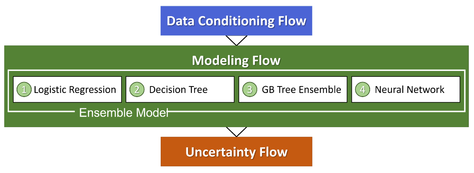
A central tenant to the workflow described here is the use of multiple ML models for predicting the favorability of a geothermal risk element. Four common, well-documented ML approaches of increasing model complexity were selected for the study (Figure 5). Specifically, we applied logistic regression (LR), a decision tree (DT), a gradient-boosted forest (XGBoost or XGB), and an ANN. Model hyperparameters, i.e., the parameters not able to be learned from data, were rigorously tuned in order to optimize the models. All models start with the same conditioned well data sets, although simplified feature subsets were derived from feature elimination or importance analysis when possible. Additional details are documented in Appendix B and in the accompanying open-source software developed by the authors [34].
2.3.1. Logistic Regression
Logistic regression predicts one of two class labels based on the weighted linear sum of the input features [41]:
where are the n feature observations, are coefficients or weights for those features, and g is the log-odds. Logistic regression adjusts the problem such that predictions define the probability of belonging to class 1. This is completed by using a non-linear logistic response function:
This equation, also known as the sigmoid function, converts the weighted sum from Equation (1) to values between 0 () and 1 () [41]. Solving for the weights () in this equation requires an iterative optimization procedure such as gradient descent. This procedure minimizes an objective function () based on negative log likelihood [42]:
The One-vs.-Rest (OVR) method was selected to extended LR to multi-class classification. OVR combines class alternatives so the number of classifiers matches the number of classes: (0 vs. (1, 2, or 3)), (1 vs. (0, 2, or 3)), (2 vs. (0, 1, or 3)), (3 vs. (0, 1, or 2)) [43]. The class with the greatest score wins, where the score is akin to the probability of class membership.
Regularization can be applied by penalizing the sum of the squared weights (-regularization) to avoid overfitting. A constant () determines the trade-off between the magnitude of the weights and negative log likelihood in the minimization [44]:
where m is the number of features. The scikit-learn LogisticRegression function used in this study applies a hyperparameter C to the negative log-likelihood term, which acts such as the inverse of [45]. Larger values of C result in less regularization [46]. See Table A1 for the final tuned hyperparameter values used for each data set.
2.3.2. Decision Trees
A decision tree classifies observations using a cascading set of evaluations, each on an individual feature from the training data set. DT models are uniquely suited to represent non-linear behavior in a highly explainable way; once constructed, the tree describes a flowchart-like map for each label assignment [41]. Only features found to be significant during tree construction will appear in the tree, ordered from higher importance features near the top to those of lower importance influencing splits near the bottom leaf nodes.
Trees are constructed by recursively performing binary splits on the training data set. Each split defines two new nodes in the tree, which correspondingly partitions a group within the training data into two subgroups. These subgroups represent new terminal leaf nodes on the decision tree. The classification decision for each leaf will be the most commonly occurring class among the training data observations assigned to that leaf [41]. Tree building takes place in two passes. In the forward pass, the tree iteratively grows by selecting nodes in the tree, a predictor to split on, and a threshold value defining the split. These choices are made to maximize the purity of the child nodes, typically using measures such as Gini index or entropy. Gini index measures variance across all K classes. Low values correspond with a strongly dominant class [47]:
where m is the subset of the training data associated with a tree node, k is a class among K possible classes, and is the fraction of all training observations in m that are of class k. Entropy also shows low values when the proportion of one class dominates and is discussed in Section 2.4 in the context of uncertainty analysis.
The tree will grow until a stopping condition is met, such as reaching a maximum tree depth or minimum number of observations allowed per node. Then, tree clean-up or “pruning” takes place in a backward pass. The following objective governs whether a tree branch is kept or removed [47]:
where refers to the number of terminal nodes in the tree. The classification error rate (E), or proportion of training samples that differ from the dominant class of a node, measures quality. acts as a regularization parameter, balancing prediction accuracy with model complexity; greater values of result in simpler trees.
A total of six hyperparameters were tuned in this study to balance the complexity of the tree with out-of-sample predictive performance when building the final DT model. Table A2 lists the hyperparameters and values determined for the different data sets.
2.3.3. Gradient-Boosted Forest
Tree-ensemble algorithms combine multiple DT models to form a more-performant forest model. Variation among the trees comes from random factors influencing their construction [47]. Gradient-boosted forests chain shallow trees in succession such that each tree predicts based on the residuals of the preceding tree. The trees are weak learners that individually underfit the data, yet when connected together, the final boosted model can outperform conventional random forests. Gradient-boosted models take the form of [47]:
where is the boosted model, are the individual trees in the chained ensemble totaling B in number, and is the shrinkage parameter or learning rate.
Extreme gradient boosting (XGBoost) is a popular variant whose objective function, governing model construction, balances two influences [48]:
where the first part () expresses how poorly the model fits the data and the second term () describes the complexity of the model. is the sum of individual loss calculations () on the n predicted and observed response variable values. Tree-specific complexity () calculations balance the number of leaves in a tree () with the L2 norm of leaf weights (), which are are unique to XGBoost decision trees. Both and serve as regularization factors.
XGBoost comes with many optimizations that make it extremely efficient, scalable, and popular among machine-learning practitioners. However, XGB models must be carefully tuned to mitigate the risk of overfitting. We focused on tuning nine hyperparameters and simplifying our feature set through importance analysis when training the XGB classifier. The specific hyperparameters and values used in modeling are listed in Table A3.
2.3.4. Neural Networks
ANNs are patterned after a simplified model of activity in the brain, where multiple inputs feed into neuron-like nodes, which pass a signal to connected nodes when an input threshold is reached [35]. The basic building blocks of ANNs act as logistic regression operators; inputs are scaled by weights, and the linear sum passes through an activation function to determine the binary output:
where h is the activation function that acts on each entry of , and is a matrix of weights. is analogous to g in (1).
The ANN cost function takes the form of a loss term and a complexity term [49]:
Here, L is the number of layers in the network, defines the number of nodes in layer , and the network prediction for the ith training observation, , consists of for all the K nodes in the output layer. represents the connection weight between node ℓ in layer and node j in layer . controls the balance between the loss and complexity terms.
The training process updates network weights using gradients calculated from the entire training data in each training round or “epoch” [35]. Successive epochs incrementally adjust the ANN to match the training data in mini-batches, that is, small subsets of the training set, rather than the whole set at once. This makes training results noisier but speeds up learning while adding a regularization effect to changes in the weights [50].
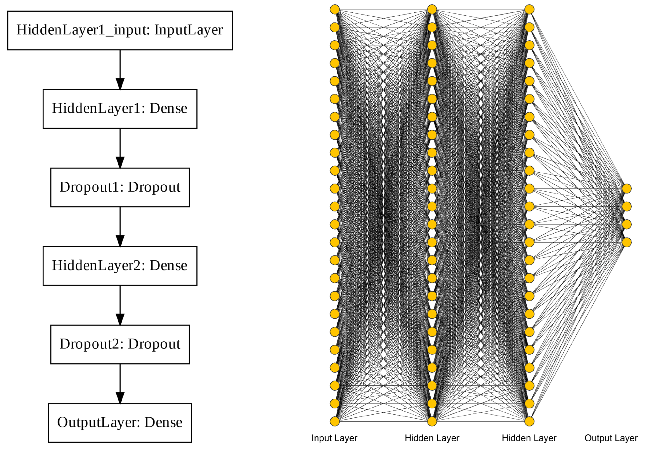
We designed a fully connected ANN with the TensorFlow Python package [51], consisting of an input layer, two hidden layers, and an output layer of four nodes representing the four geothermal gradient classes being predicted (Figure A28). The hidden layers use ReLU (rectified linear unit) activation functions, and the AdaM (adaptive moment) optimization method was selected for the training process [52,53]. In addition to network architecture choices, we tuned a total of five hyperparameters for the final classifier. The list of hyperparameters and values selected for each well data set is provided in Table A4.
2.3.5. Feature Importances
Similar to the natural ranking observed in decision trees, feature importance algorithms reveal ML model sensitivity to different feature inputs. The ShAP (Shapley additive explanations) method predicts importances without assuming complete feature independence [54]. In addition, average ShAP values capture global significance for general feature importance, while individual values have local significance for single point predictions. The sum of ShAP values equates to the deviation of the model prediction from the average value (baseline), meaning ShAP values describe the individual feature contributions to a prediction value [54]. In this study, we used ShAP analysis for feature simplification when tuning the XGB model, but we also show how ShAP results can support resource-constrained decisions for geothermal exploration activities.
2.4. Uncertainty Analysis Workflow
We evaluate the performance of each ML classifier using percent correctly classified (accuracy), a confusion matrix of actual and predicted class labels, and evaluating the trade-off in true-positive rate and false-positive rate as a function of decision threshold for class assignments. The latter function defines the receiver operating characteristic (ROC) curve, which is often summarized by its integral, the area under the curve (AUC) [55]. In addition to these, we use the concept of Shannon entropy as a proxy for classification uncertainty [56]:
where x represents a single observation location and is the conditional probability assigned to class by the classifier. Although this normalized entropy calculation does not account for the sequential relationships between the geothermal gradient classes, it exhibits good discrimination ability for model results that show different levels of stand-out between the assigned (highest) class label score and the scores for alternative class labels [57]. Therefore, an entropy map constructed for a single classification model can illustrate the spatial variability in the relative prediction uncertainty for that model.
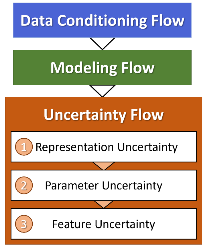
Our analysis builds on this concept to explore uncertainties from three different sources in this study: algorithm selection (representation), model calibration during the learning process (parameter), and input data variance and interpolation (feature), which are presented as a workflow in Figure 6. In each case, the uncertainty is estimated from an ensemble of model results. Both an aggregate model prediction and a set of class label scores for each location in the study area are derived from this ensemble.
Among the many options for combining multiple classifier outputs, we selected distribution summation, whereby the arrays of conditional probabilities from each classifier are summed, and the ensemble prediction is the label with the highest value in the total array [58]:
where x represents the feature values for an observation, are the K possible class labels, and are the conditional probabilities of all possible classes as predicted by model .
2.4.1. Representation Uncertainty
One consequence of representing complex systems such as geothermal resource prediction by a single ML algorithm is the constraints it places on exploring the solution space due to underlying model assumptions, the form of the model objective function, and the optimization methodology employed. Rather than focus on a single “best” model, the four classifiers presented in Section 2.3 were combined for an aggregate or ensemble prediction using the distribution summation method (12). Then, representation uncertainty for the model ensemble was calculated using entropy (11) at each map location in the study area.
2.4.2. Parameter Uncertainty
Fitting supervised ML models to training data typically requires iterative updates to model parameters based on objective-function optimization. However, the final trained models treat learned parameters as deterministic with no uncertainty. Probabilistic algorithms such as Bayesian neural networks (BNN) replace single parameter values with probability distributions [59]. A fully-trained BNN samples from these distributions for just-in-time determination of node weight values as data are fed-forward to produce a prediction.
In this study, we constructed a BNN by replacing the second hidden layer of the ANN model in Section 2.3.4 with a probabilistic layer using the TensorFlow Probability Python package (Figure A29) [60]. We chose to replace just one layer of the ANN as a balance between the limited size of the training data sets and the explosion in parameter count each probabilistic layer brings to the BNN architecture. A suite of results was generated via 1000 model predictions on the same input data. Then, we applied the distribution summation method (12) to derive an array of class scores and calculated entropy values (11) that characterize parameter uncertainty for the neural network model.
2.4.3. Feature Uncertainty
Only a fraction of the features obtained from public sources in this study were already pre-conditioned and were complete raster files ready for modeling and analysis (Table 1). Interpolation steps taken to convert a point set, polyline set, or incomplete grid into the format required can propagate uncertainty into the prediction problem. Furthermore, feature standard errors, generally overlooked by traditional ML methods, contribute to an overall feature uncertainty estimate.
Using a single feature as a proof-of-concept, we estimated standard errors with empirical Bayes kriging (EBK), which is a probabilistic interpolation method that also accounts for multiple measurements at one location [61]. Next, a derived data set was created by adding random Gaussian noise to the feature GIS map based on the spatially variant feature standard errors. Repeating this process 100 times generated input data sets that are statistically consistent with the original feature values. As with the other uncertainty estimates, the ensemble of results from training and predicting on these data sets was combined using distribution summation (12), and uncertainty was characterized by calculating entropy (11). Although we applied this procedure to a single feature, it could easily be extended to investigate how uncertainty related to multiple features can influence the uncertainty in the final model results.
3. Results
3.1. Individual Models
The LR, DT, XGB, and ANN machine-learning models were each tuned and trained on the three well data sets in succession. Table 5 lists the in-sample (training) and out-of-sample (test) results using accuracy and AUC metrics for all models and data sets. The more complex XGB and ANN models show fewer misclassifications across all geothermal-gradient classes than the simpler LR and DT models. There is a demonstrated uplift in model performance between the original WDS data set and the augmented WDS4 and WDS8 data sets for all models. However, we do not observe significant or consistent improvement from using WDS8 over WDS4—the benefits of training on augmented data are realized with the smaller WDS4 data set, and additional pseudowells do not noticeably improve classifier performance metrics for WDS8. Therefore, WDS4 results are used as the focus of the analysis for the remainder of this study.
Model results are further characterized by the confusion matrices in Figure 7. All models produce several predictions off by a single sequential class assignment for the test data, the most prevalent being between the medium-grade (class 2) and high-grade (class 3) geothermal gradient. The LR model is more prone to misclassifications of two or more sequential classes, including some locations marked as high-grade that actually fall in the non-geothermal (class 0) category. The ANN model performs best in that it misclassifies by no more than a single sequential class. However, aside from three high-grade false positives that should be low-grade, the XGB model also does very well.
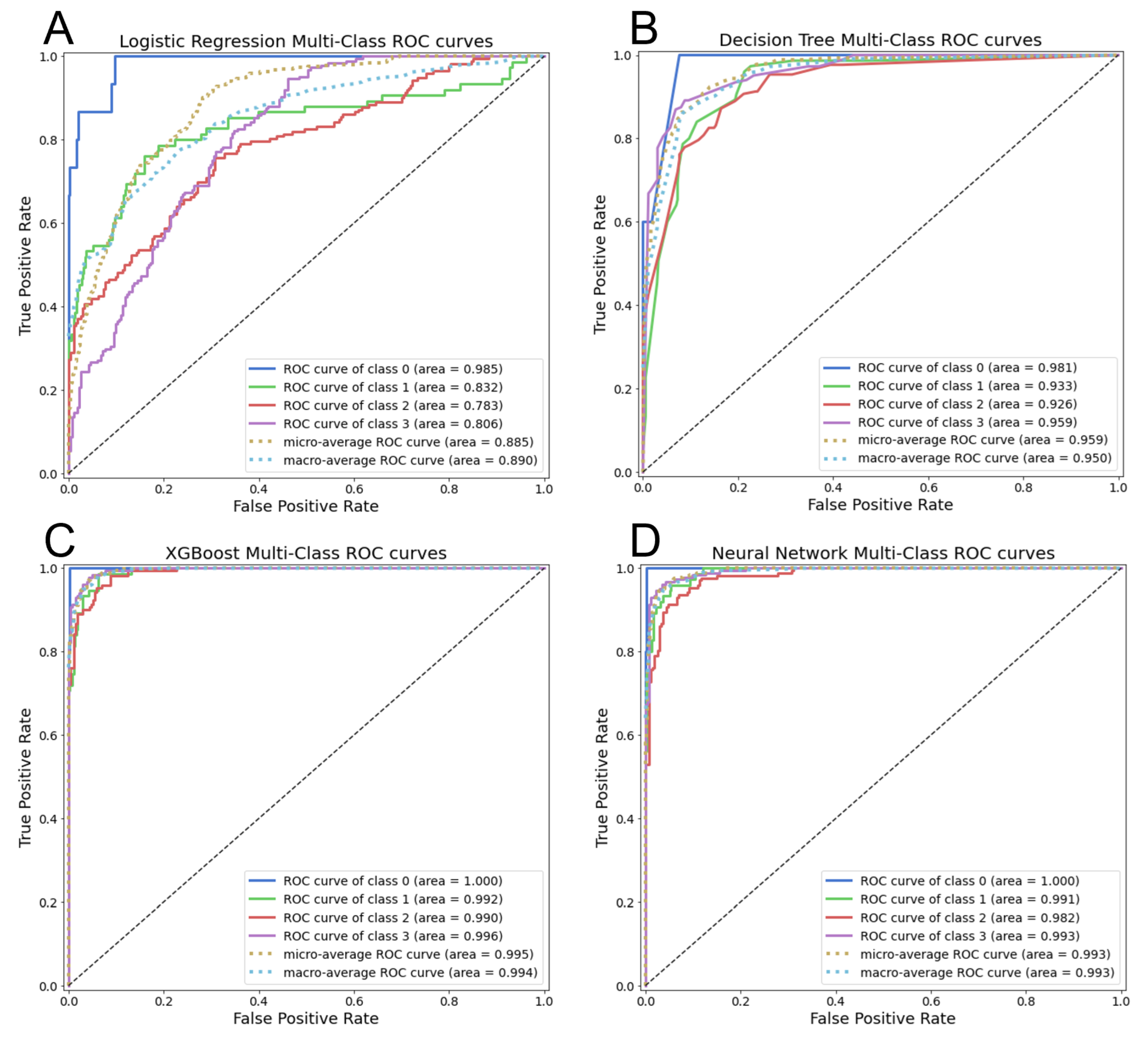
Figure 8 illustrates the individual class, micro-average, and macro-average ROC curves based on the predicted scores for each class label. Ideal models minimize the false-positive rate while maximizing the true-positive rate for all classifier decision thresholds, meaning they plot in the upper-left corner. These plots effectively demonstrate the predictive strength of both the XGB and ANN models compared to the DT and LR models. The classification performance for class 2 lags behind other individual classes. This suggests that the mid-grade geothermal gradient is more difficult to uniquely distinguish with the feature data.
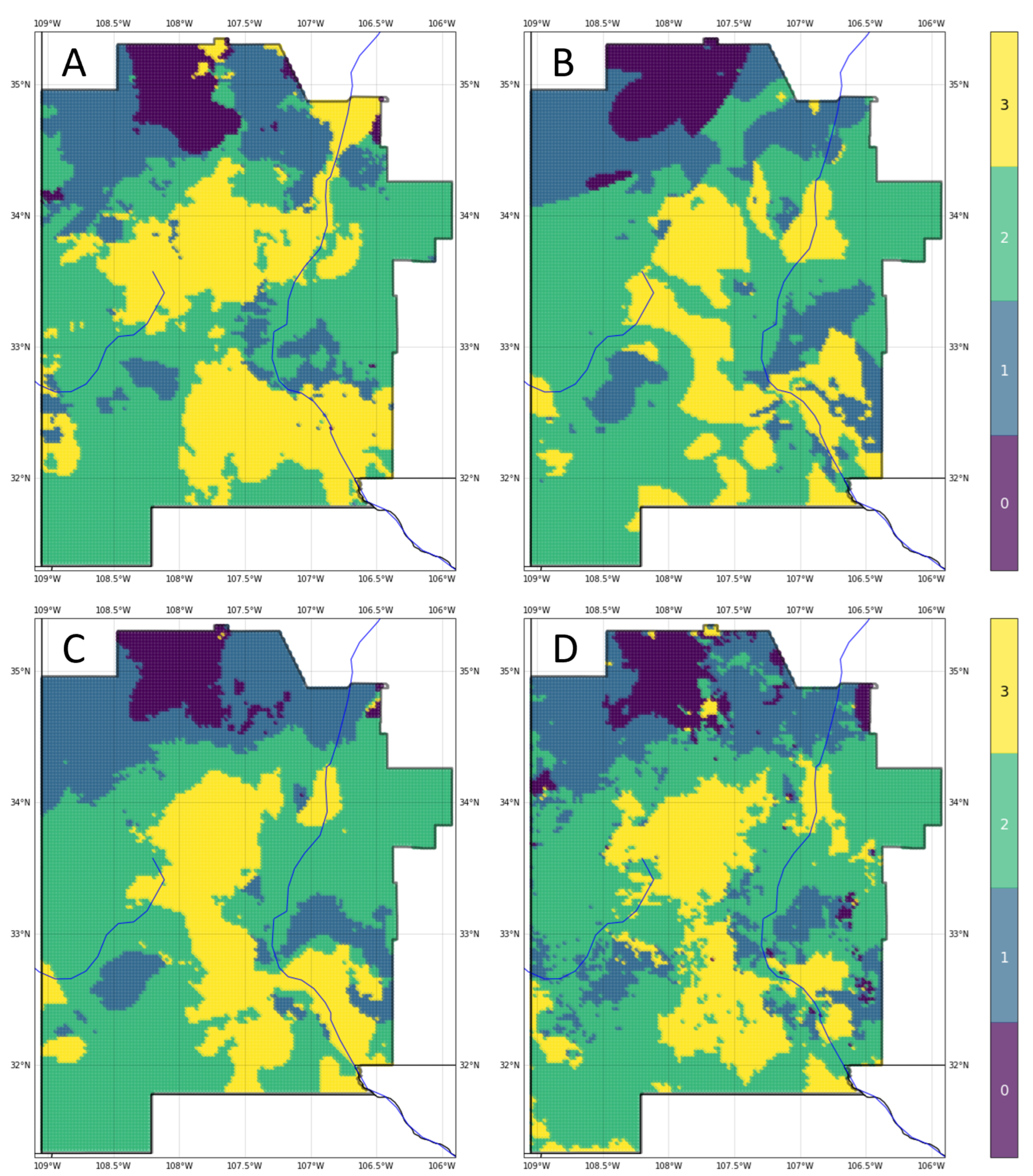
Values from the input feature maps were extracted using a grid of points spaced within the AOI; then, they were fed into each classifier to generate geothermal gradient maps for southwest New Mexico (Figure 9). The similarity of gross play fairway trends across different machine-learning results is striking, as is the unique signature style of prediction that each algorithm produces. Individually, the maps offer actionable guidance for an exploration team on potential prospect targets. However, collectively, they also indicate the uncertainty in the geothermal gradient predictions both for the broader trends and in local details.
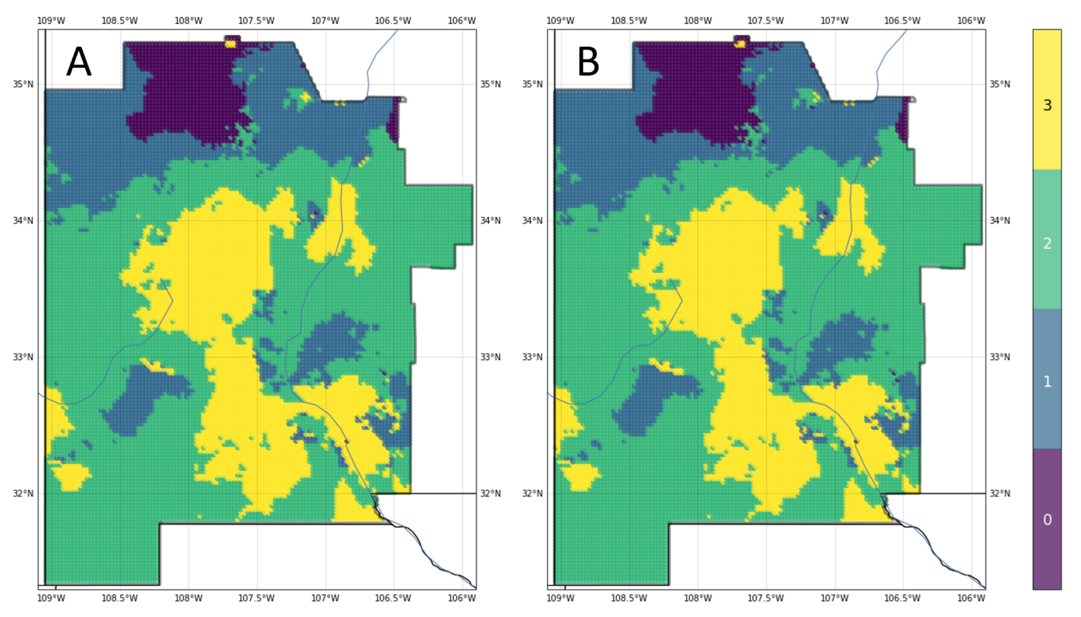
To examine this further, we created the ensemble prediction map in Figure 10A using distribution summation (12) at each of the extraction-grid coordinate locations within the AOI (x in the equation). The ensemble model demonstrates stronger predictive performance than the individual models based on an out-of-sample AUC of 0.995, and it bests all but the ANN model with an out-of-sample accuracy of 0.942. Figure 10B depicts predictions when a weighted average scheme using test set accuracy is applied during distribution summation. Although the differences between the two maps in Figure 10 are subtle, the weighted model improves the results even further: WDS4 out-of-sample accuracy grows to 0.955 and AUC climbs to 0.997.
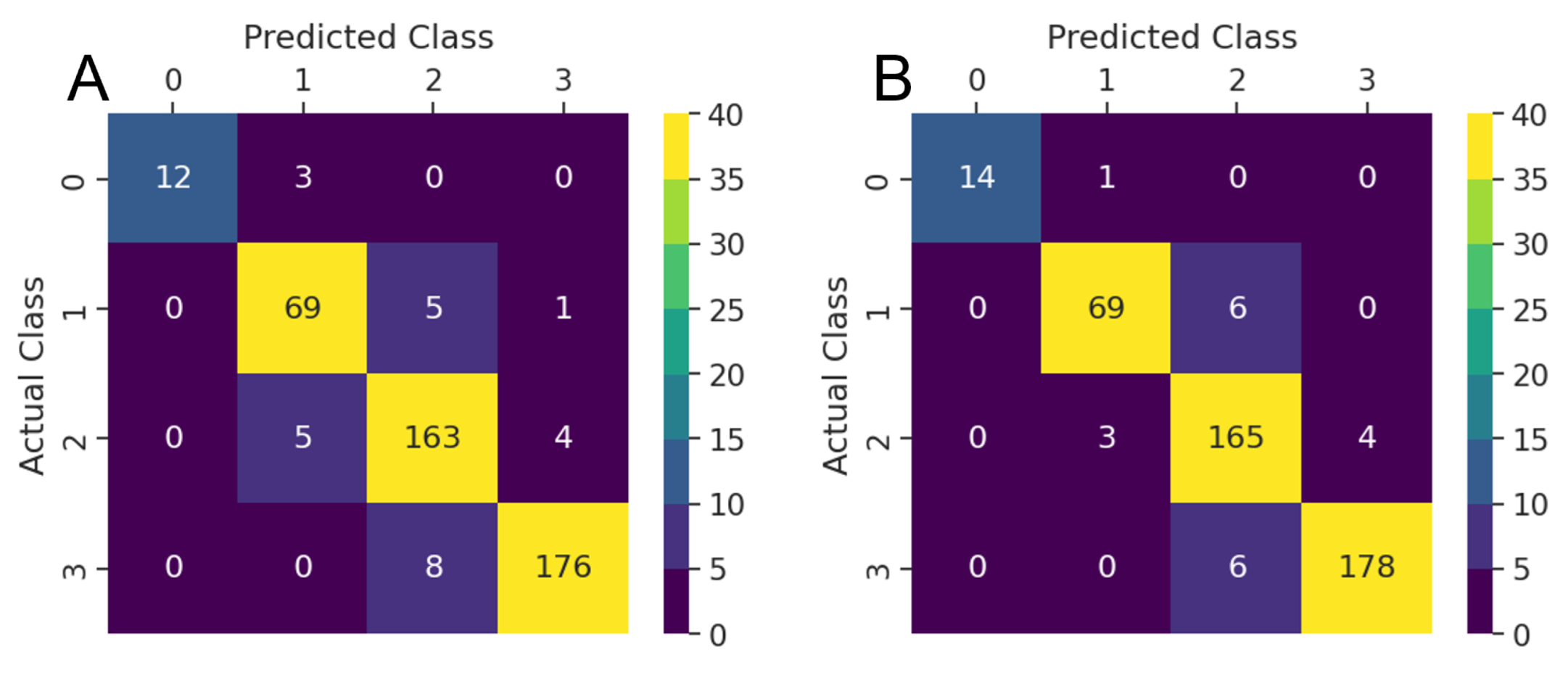
Figure 11 shows the confusion matrices for both the unweighted and weighted average four-model ensemble classifiers. Based on these observations, the best results come from applying a weighting scheme on the distribution summation, allowing all models to contribute to the ensemble but also taking into account the measurable performance differences between the models.
3.2. Representation Uncertainty
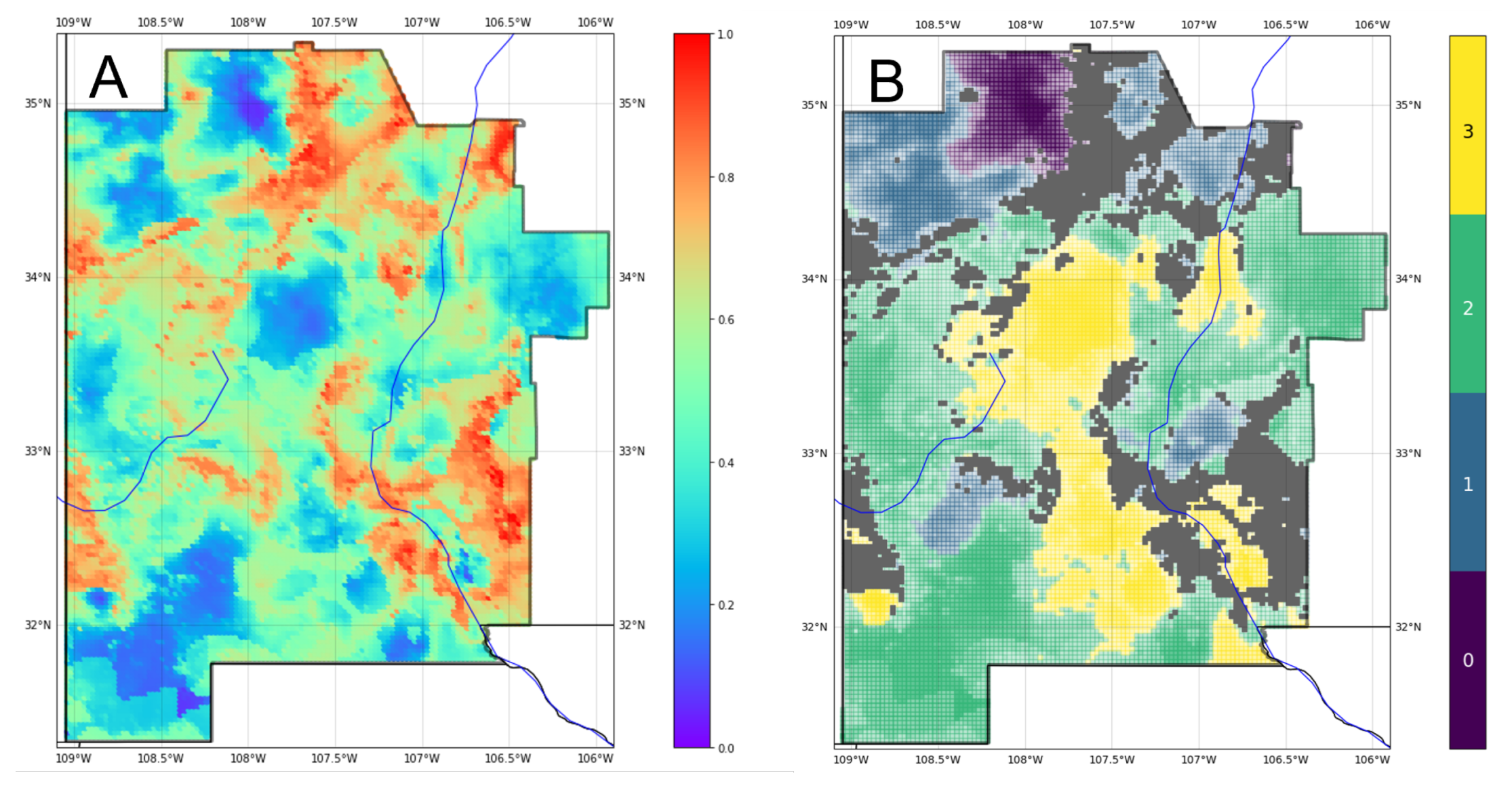
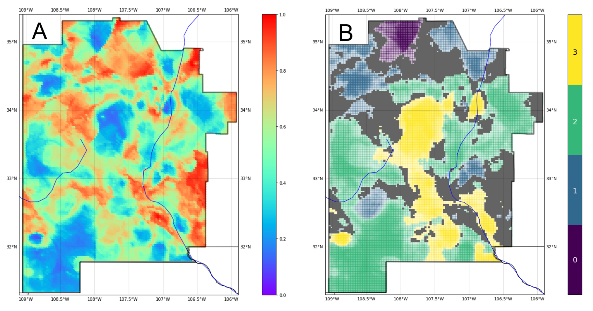
Figure 12A depicts a map of relative uncertainty in the form of Shannon entropy (11) calculated at each AOI grid location. Areas where normalized entropy reaches a value of 0.7 or greater are masked out (gray) in the ensemble prediction map (Figure 12B), and lower levels of entropy imply less transparency of the four class colors to communicate both uncertainty and classification results. This figure provides multiple levels of information to an exploration team. The high temperature-gradient areas identify prospects for shallower heat resources to target in an exploration program. Additionally, the masked regions indicate where the models cannot differentiate between two or more class labels. Rather than bias a team on the gradient potential of high-entropy regions with a highly uncertain classification, we allow the mask to communicate that no judgment call should be made without further study.
3.3. Parameterization Uncertainty
The Python TensorFlow implementation of the ANN model includes a total of 1300 trainable parameters that must be learned during model training. Summary statistics (Table 5) suggest the ANN is a reliable classifier for the entire southwest New Mexico study area. However, with so many parameters to learn and such limited training data to learn from (Table 3), we chose to test this assumption using the BNN approach. Figure 13 illustrates the entropy map derived from 1000 predictions from the BNN tuned and trained on WDS4, as well as a results ensemble map with uncertainty masking as described in Section 3.2.
Uncertainty from the model parameterization is not spatially uniform; patches of high entropy are concentrated to the southeast where the predicted geothermal gradient—and ground truth well measurements (Appendix A.26)—vary significantly over short lateral distances. The high-grade geothermal-gradient region in the center of the AOI demonstrates low entropy values, indicating that the trained neural network model has enough parameter certainty to predict a positive heat resource classification in this area consistently.
3.4. Feature Uncertainty
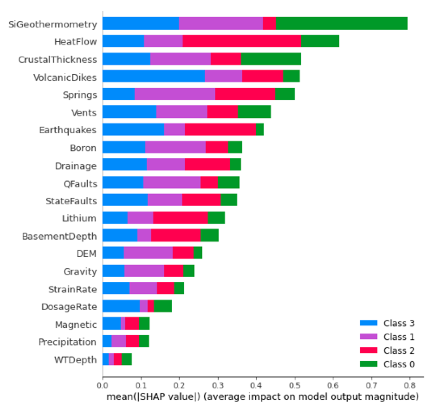
Figure 14 illustrates feature importances for predictions of a geothermal gradient derived from ShAP analysis. This analysis focuses on the XGB model due to its high performance among the classifiers studied and the integration in Python toolkits for both XGBoost prediction and Shapley value calculation [62,63]. The three features with the greatest average ShAP magnitudes across all test data locations and gradient classes are Si geothermometer temperature (SiGT), heat flow, and crustal thickness. By inference, uncertainty in the values for these features should most strongly translate into uncertainty in the final classification results. To investigate this further, we applied the EBK method to derive standard error estimates for the globally most important feature, SiGT; then, we applied the feature uncertainty approach to testing the sensitivity of prediction results to this feature. Note that ShAP values for individual classes can vary from the global assessment. For example, the most important feature for class 3 is volcanic dike density, while heat flow is most important for class 2. Therefore, the uncertainty analysis can be tailored depending on the specific class of greatest interest to a geothermal project team.
The normalized entropy map in Figure 15 was created using XGB predictions for 100 variations of WDS4, each including SiGT perturbed by Gaussian noise calibrated to SiGT standard errors. Large spatially contiguous patches of high entropy to the northeast, southeast, and elsewhere highlight areas where variance in SiGT values results in significant uncertainty for the ML models. Assuming this represents epistemic uncertainty, the entropy map provides important guidance for a mitigation strategy; collecting additional data in the masked regions could reduce SiGT feature uncertainty and thus increase confidence in the classifier results due to the importance of this feature.
4. Discussion
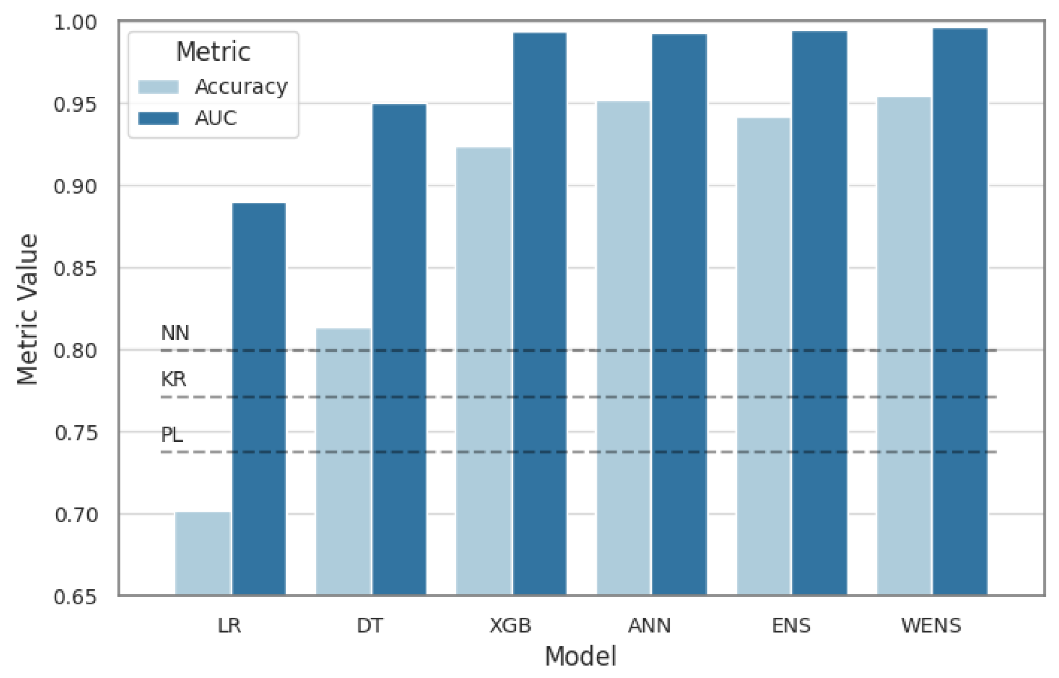
Although similar in regional trends, each of the four supervised ML methods presented in Section 3.1 show differences in local predictions and overall performance as geothermal gradient classifiers. The weighted-average ensemble model demonstrates better performance than the individual models alone, supporting an argument for ensemble approaches to the ML-enhanced PFA methodology. Figure 16 summarizes the comparison between the ML models based on test set accuracy and AUC.
A vital additional comparison must address whether or not ML provides meaningful uplift over conventional methods used in PFA workflows. For the southwest New Mexico study area, the prior PFA predicted an integrated favorability assessment for hydrothermal resources, not enthalpy alone [16]. Nevertheless, PFA data uploaded to the open-access Geothermal Data Repository include an interpolated map of geothermal gradient based on well data similar to those included in this study [17]. Using the PFA as a baseline, we consider interpolation as the the primary alternative to predicting temperature gradient with ML techniques. More precisely, a comparison can be made between the ML results and those for interpolation functions constructed using the WDS training subset and evaluated against the remaining WDS data points. This assessment was performed using three algorithms: piecewise-linear interpolation and nearest-neighbor interpolation from the scipy Python library [64], and ordinary kriging with a spherical variogram model available in ArcGIS. These methods provide deterministic estimates of gradient for the combined WDS validation and test subsets, which were then converted to the classification scheme in Table 2 for comparison with the ML models. AUC cannot be calculated, but interpolant accuracy scores fall short of those achieved by all but one individual ML model (Figure 16), and they are well below the ensemble model accuracies.
It is important to note a fundamental difference between the two estimation methodologies: interpolation algorithms predict geothermal gradient from the spatial relationships embedded in the training data, while the ML models learn from signals within the features listed in Table 1, which notably do not include geospatial coordinates. Not only does the ML workflow result in better predictions, those predictions are data-driven at each map location rather than spatially derived. This narrow focus in detection may be particularly advantageous for identifying blind geothermal systems whose presence and bounds can be highly local in nature.
However, presenting the individual and ensemble results to explorationists interested in prospect identification and maturation would invariably elicit two important questions: (1) how much confidence should be assigned to the class labels agreed by only a plurality of models, and (2) what would be the best next steps to take based on these models. At the heart of the first question is the need to pair the use of ML methods with uncertainty characterization, specifically uncertainty due to different model representations and where those models fail to agree in classifications. Incorporating several high-performance models into an ensemble estimate with an uncertainty metric such as entropy can give a geothermal exploration team confidence in which areas should receive more attention and resources, either in data purchases, new data acquisition campaigns, or hours of traditional play fairway and prospect interpretation activities.
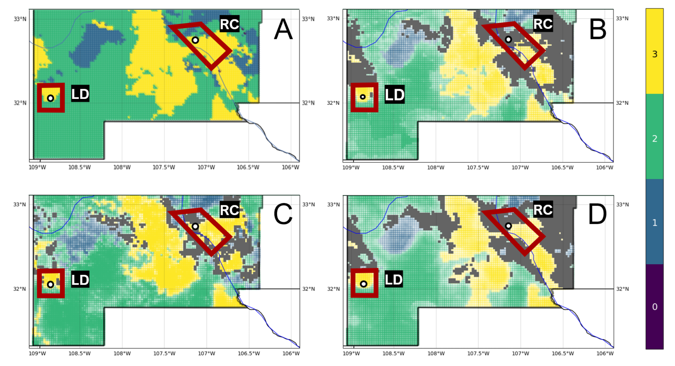
The workflow described in Figure 6 notes multiple sources of uncertainty, each with the potential for providing meaningful information in translating predictions into exploration decisions. To illustrate this point, we consider the scenario where the hypothetical prospect outlines identify two areas of interest, Lightning Dock (LD) and Rincon (RC), for an EGS installation within the southern half of the study area (Figure 17). The ensemble classifier predicts high-grade enthalpy resources, approximated by geothermal gradient, within either quadrangle (Figure 17A). Note that the primary risk element for EGS is enthalpy, since permeability and fluids solutions could be engineered. White markers indicated reference points as proposed drill locations, which are presumably influenced by additional factors such as access to transmission lines, infrastructure, or permitting constraints. With no additional information, LD and RD would rank equally high in prospect favorability.
Model representation uncertainty reveals a greater level of confidence in the gradient prediction at LD compared to RC (Figure 17B). Masked values at the RC reference point indicate high entropy, suggesting that the project team should explore options to obtain more information and rerun the ML PFA workflow with any additional data. If no additional information is available, the team could either adjust their risk tolerance on RC, focus further subsurface characterization efforts on this region, or choose to abandon RC as a prospect altogether, since the ML models cannot clearly differentiate among gradient classes with the available feature data.
Shifting focus to the ANN classifier as one of the top-performing models, an analysis of parameterization uncertainty shows low entropy across most of both the LD and RC quadrangles (Figure 17C). However, the reference point for RC lies along a narrow northwest–southeast trend of high entropy. The project team could choose to adjust this proposed well location slightly east or west to avoid this trend while staying within a Class 3-labeled region. Alternatively, an ML model with fewer trainable parameters may be a more appropriate choice for RC predictions, in addition to traditional subsurface interpretation and modeling efforts, to help mitigate the risk of this prospect.
Uncertainties tied to the feature of highest importance, SiGT, also offer useful insights into this hypothetical prospect evaluation. Entropy levels appear quite low at LD and marginally high at the RC reference point (Figure 17D). High entropy throughout the northern section of the RC quadrangle could be mitigated with additional silica concentration sampling in the field. A closer review of SiGT data in the RC area might prove beneficial as well. Anomalous values in the original data, if they are erroneous, will increase standard errors, impacting both the EBK interpolation routine and overall predictive value of the feature. On the other hand, anomalous values that are trustworthy must be accepted as indicators of strong lateral heterogeneity. Thus, uncertainties here can contribute to an important feedback loop for appropriate data conditioning, which is the key first step in the ML-enhanced PFA workflow.
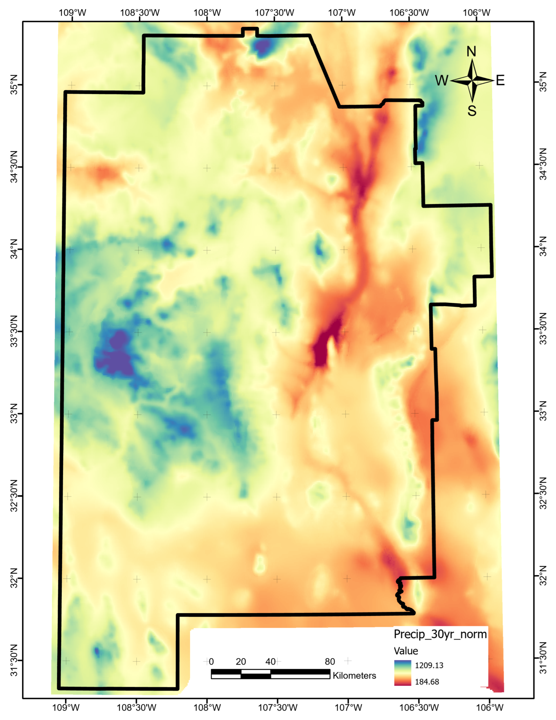
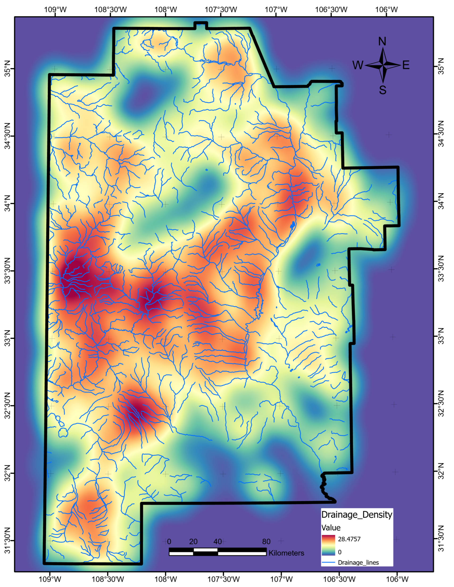
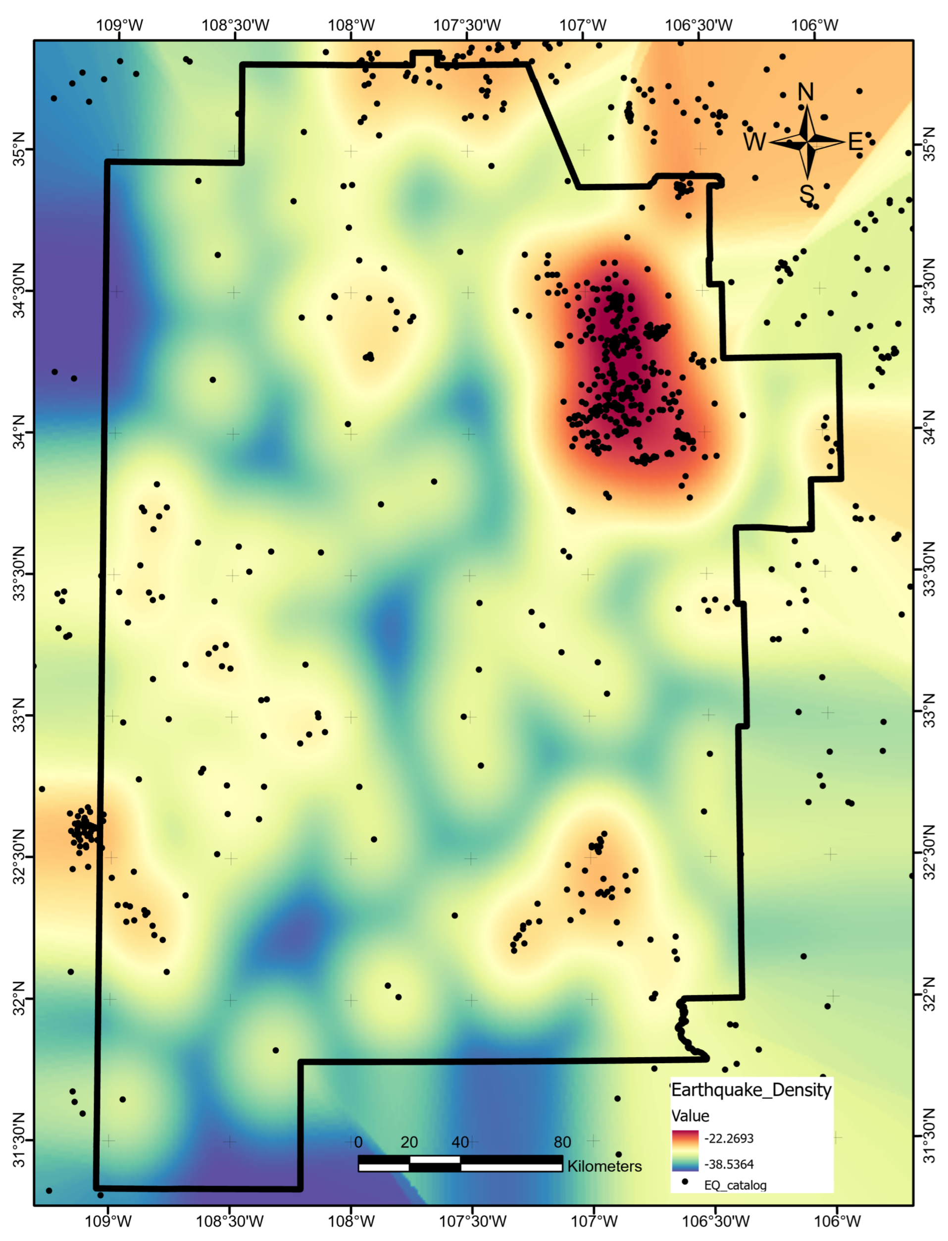
The optimal allocation strategy for geothermal-project resources should also take the full feature importance analysis results into account. Average ShAP magnitudes for water table depth, average precipitation, and magnetic anomalies rank lowest among the features in this study (Figure 14). The poor predictive value of these data sets would not justify additional project time or budget appropriations targeting their collection or analysis. Similarly, water-table gradient, topographic gradient, gravity-anomaly gradient, and magnetic-anomaly gradient do not even appear in the ShAP value sensitivity report and could reasonably be set aside as low priority data sets. Instead, spending should focus on high-value data, including fault and drainage maps; the earthquake catalog and heat-flow estimates; mapped vents, springs, and volcanic dikes; crustal thickness estimates; and boron and silica concentrations. Note that feature importance rankings will likely vary from locality to locality if the local geophysical configurations are just sufficiently different, or even in the same project area if features are replaced with newly acquired or reprocessed data. Insights from ShAP analysis apply to models trained on a particular feature set and would necessarily require a refresh should that feature set or the geophysical configuration change.
5. Conclusions
The objective of this paper was to revisit the play fairway analysis (PFA) methodology and apply machine learning (ML) models for risk element prediction, uncertainty estimation, and decision guidance for a geothermal project team in the exploration phase of field development. Fundamentally, this process successfully resulted in classification maps of geothermal gradient, a proxy for subsurface enthalpy resource presence, covering the study area in southwest New Mexico. Maps were generated from four separate machine learning methods and from a weighted ensemble model that demonstrated better overall predictive performance. The ensemble also outperformed common interpolation routines that only rely on spatial patterns for prediction. Variance in the individual ML classifier results within the ensemble is rooted in different underlying distributions of the class probabilities based on the chosen model representations. We applied distribution summation on the class probabilities and calculated entropy to quantitatively measure spatial locations where ensemble predictions had high confidence or where ensemble results could not be trusted due to this representation uncertainty. Incorporating probabilistic components into ML models allows parameterization uncertainty to be measured in a similar way. This measure helped us identify areas in the case study where the neural network may be under-constrained due to lack of sufficient training data or iterations. Standard errors in the input features define a third source of uncertainty that is easily measurable using a solution ensemble and entropy approach. When applied to features that rank highly in an importance analysis, such as silica geothermometer temperature in southwest New Mexico, feature uncertainty can provide clear guidance on locations where information gain from data-gathering activities would be of the highest value.
We believe applying these steps in a comprehensive ML-enhanced PFA strategy for mapping enthalpy favorability can influence conventional hydrothermal, enhanced geothermal systems, and even advanced closed loop geothermal exploration projects. Further enthalpy resource characterization would also need to take other parameters, such as thermal conductivity, into account. Furthermore, practitioners should extend the workflow for pre-screening other risk elements such as permeability and fluids for a complete PFA depending on the targeted type of geothermal system. One further caveat must also be addressed: ML-enhanced PFA methods cannot replace subject matter experts in geothermal exploration. Rather, the methods proposed here give practitioners valuable decision support for more efficient project execution. The associated data-driven insights enable highly targeted technical efforts and rapid identification of prospects, both of which are requirements to support future growth of the geothermal industry.
Author Contributions
Conceptualization, R.C.H. and A.F.; data curation, R.C.H.; formal analysis, R.C.H.; investigation, R.C.H.; methodology, R.C.H.; software, R.C.H.; supervision, A.F.; visualization, R.C.H.; writing—original draft preparation, R.C.H.; writing—review and editing, A.F.; All authors have read and agreed to the published version of the manuscript.
Funding
This research received no external funding. Publication of this manuscript was funded by Chevron.
Data Availability Statement
The data presented in this study are openly available in multiple publicly accessible repositories as described in Table 1 and Appendix A. The software used in this study is openly available in GitHub [34].
Acknowledgments
We would like to thank J.E. Faulds, M.C. Fehler, S.R. Brown, J.H. Queen, W.L. Rodi, C.M. Smith, and S. Trietel for engaging discussions on machine learning applied to PFA; J.D. Pepin for discussion and data pertaining to his thesis; M.C. Edwards and J.A. Nunn for insightful draft reviews; and the three anonymous reviewers for their helpful comments.
Conflicts of Interest
The authors declare no conflict of interest. The funders had no role in the design of the study; in the collection, analyses, or interpretation of data; in the writing of the manuscript, or in the decision to publish the results.
Abbreviations
The following abbreviations are used in this manuscript:
| ACL | Advanced Closed Loop |
| AOI | Area of Interest |
| ANN | Artificial Neural Network |
| AUC | Area Under the ROC Curve |
| BNN | Bayesian Neural Network |
| DT | Decision Tree |
| EBK | Empirical Bayes Kriging |
| EGS | Enhanced Geothermal Systems |
| GIS | Geographic Information System |
| KGRA | Known Geothermal Resource Area |
| LR | Logistic Regression |
| ML | Machine Learning |
| OVR | One-vs.-Rest |
| PFA | Play Fairway Analysis |
| ROC | Receiver Operating Characteristic |
| SiGT | Silica Geothermometer Temperature |
| SMU | Southern Methodist University |
| WDS | Well Data Set |
| XGB | eXtreme Gradient Boosting (XGBoost) |
Appendix A. Feature Data Layers
All features used as predictor and response variables for the ML workflow required some preparation prior to modeling. For each feature below, we describe the source of the data, outline the conditioning steps applied to the data, and provide an image of the final GIS map.
Appendix A.1. Average Air Temperature
The University of Oregon PRISM Climate Group maintains regularly updated spatial data sets of climate-related observations, including 30-year average annual conditions [18,38]. We downloaded the 800 m resolution average air-temperature grid and cropped to the study area (Figure A1). This layer required no further processing.
Figure A1.
Average air temperature data layer map, produced using ArcGIS Pro. Units are C. Data were retrieved from the PRISM website [18].
Figure A1.
Average air temperature data layer map, produced using ArcGIS Pro. Units are C. Data were retrieved from the PRISM website [18].

Appendix A.2. Average Precipitation
We also downloaded the 800 m resolution 30-year average-precipitation grid from the PRISM Climate Group [18,38]. This layer required no additional processing after cropping it to the study area (Figure A2).
Figure A2.
Average-precipitation data layer map, produced using ArcGIS Pro. Units are millimeters. Data were retrieved from the PRISM website [18].
Figure A2.
Average-precipitation data layer map, produced using ArcGIS Pro. Units are millimeters. Data were retrieved from the PRISM website [18].

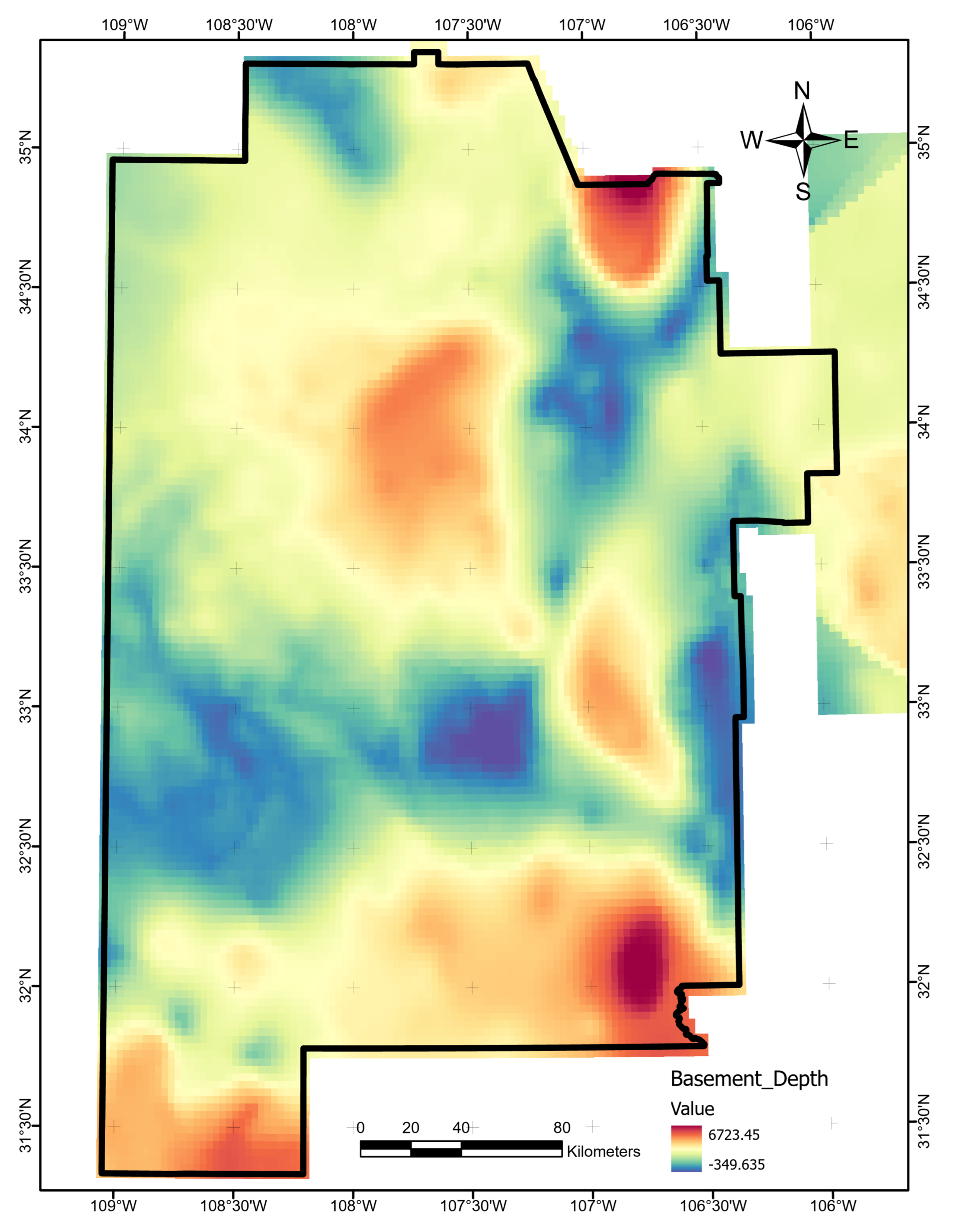
Appendix A.3. Basement Depth
Following the procedure outlined by Pepin [9], we used the basement-elevation raster created by Bielicki et al. [16] to calculate depth to basement. First, we extracted values using a grid, which revealed patches of missing data. These values were replaced using ordinary kriging with a spherical semivariogram model, lag size of , and a variable search radius requiring four neighboring points. We filtered the Surface Topography (DEM) layer by averaging across a neighborhood to suppress detailed surface morphologies. To make the final basement elevation layer, we subtracted the interpolated basement elevation layer from the filtered DEM (Figure A3).

Appendix A.4. Boron Concentration
Measurements of boron concentration were collected by Bielicki et al. [16] from USGS records, student dissertations, and other sources. After obtaining these point data, we merged them into a single collection of 5686 measurements constrained to the southwestern New Mexico region. Interpolation of the data was performed using empirical Bayes kriging (EBK), which manages both non-uniform spatial distributions and multiple values from locations where repeated samples were taken [61]. We used EBK with K-Bessel semivariograms and a maximum of 100 points in 100 simulations to generate the final data layer (Figure A4). Note that unlike some interpolants, kriging produces piecewise continuous surfaces with zero-order continuity at patch borders [65]. There is no constraint to enforce globally smooth surface solutions, which explains sharp lateral gradients in kriging maps such as this one.

Appendix A.5. Crustal Thickness
In the absence of a more recent seismic study constraining variations in crustal thickness across the study area, we used the regional map published by Keller et al. [19] to construct the crustal-thickness feature layer. Following the procedure described by Pepin [9], we digitized the thickness contours from the Keller map, then interpolated between them using the ArcGIS Topo to Raster function, which uses an iterative finite difference method and removes local minima not supported by the input data [66]. The resulting map in Figure A5 shows an appropriately long-wavelength approximation for regional crustal-thickness variations given the original sparse constraints from 2D seismic lines shot in the 1960s–1980s [19].
Figure A5.
Crustal-thickness data layer map, produced using ArcGIS Pro. Units are kilometers. Black lines trace contours digitized from Figure 4 in [19], extrapolated outside the AOI to the west for gridding purposes.
Figure A5.
Crustal-thickness data layer map, produced using ArcGIS Pro. Units are kilometers. Black lines trace contours digitized from Figure 4 in [19], extrapolated outside the AOI to the west for gridding purposes.

Appendix A.6. Drainage Density
We obtained drainage polyline data from the original PFA submission to the OpenEI repository [17]. In converting line data to into a feature map, we elected to use a kernel density estimation technique that fits smooth surfaces over each line, maintaining a maximum value along the line length and a radius-controlled decay to either side [67]. The final drainage density layer (Figure A6) used a radius of .

Appendix A.7. Earthquake Density
Following the procedure outlined by Pepin [9], we created a southwest New Mexico earthquake catalog by combining historical earthquake records for the years 1869–1998 [20], 1999–2004 [21], and 2005–2009 [22] with data pulled from the USGS earthquake catalog [23]. The final study area collection comprised 2539 unique events spanning 1962–2020. We used a grid search routine with 10-fold cross-validation to determine the best search radius of 11,600 m for an earthquake kernel-density estimate (KDE). The final data layer is shown in Figure A7.
Figure A7.
Natural logarithm of earthquake density in number per km. Map produced using ArcGIS Pro. Black dots indicate earthquake event point locations.
Figure A7.
Natural logarithm of earthquake density in number per km. Map produced using ArcGIS Pro. Black dots indicate earthquake event point locations.

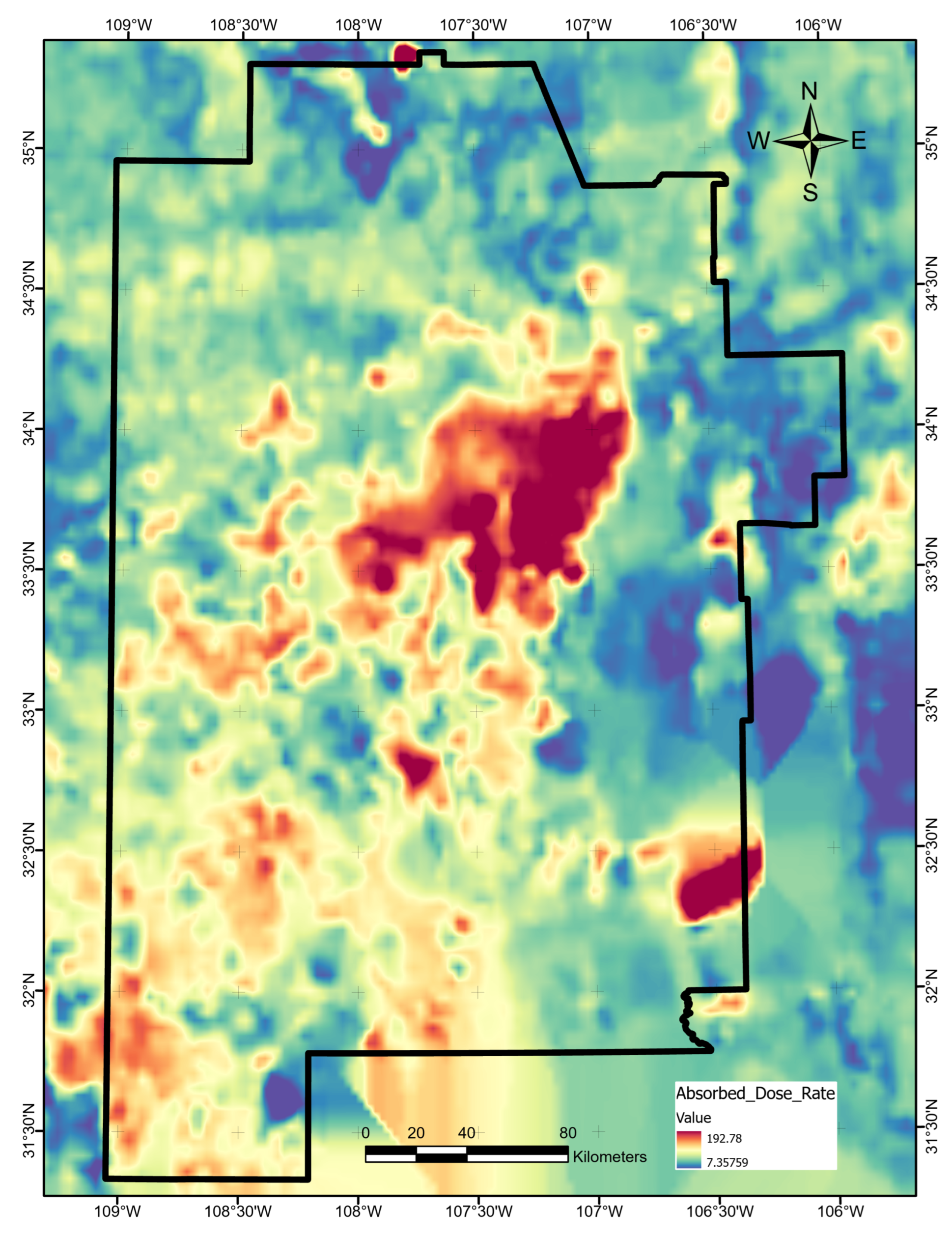
Appendix A.8. Gamma-Ray Absorbed Dose Rate
Aerial gamma-ray surveys conducted across the United States in the late 1970–1980s are the basis for Potassium (K) concentration (in percent K), equivalent Uranium (eU) concentration (in ppm), and equivalent Thorium (eTh) concentration (in ppm) maps. These measures collectively define the absorbed dose rate, which can be calculated from the following equation: [24].
We obtained the absorbed dose rate for West Central USA from the USGS Open-File Report 2005-1413 website [24] and cropped it to the southwest New Mexico area. Then, we filled a data gap near the White Sands Missile Range by using ordinary kriging with a spherical semivariogram model, lag size of , and a variable search radius requiring four neighboring points. Figure A8 illustrates the final map.
Figure A8.
Absorbed dose-rate data layer map, produced using ArcGIS Pro. Units are nanograys/hour. Original data from USGS Open-File Report 2005-1413 [24].
Figure A8.
Absorbed dose-rate data layer map, produced using ArcGIS Pro. Units are nanograys/hour. Original data from USGS Open-File Report 2005-1413 [24].

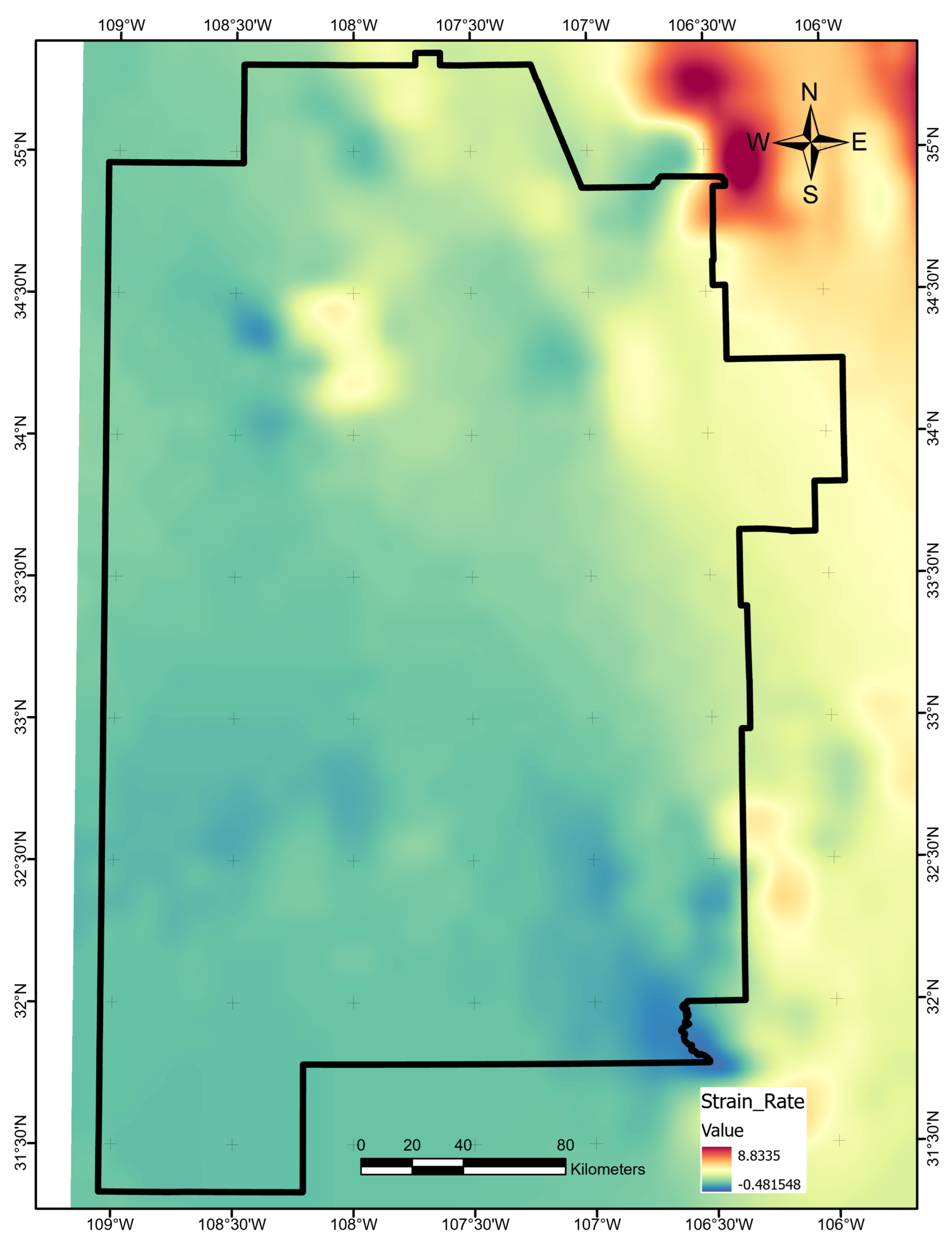
Appendix A.9. Geodetic Strain Rate
We downloaded the global strain rate model (GSRM) v.2.1 [25] directly from the University of Nevada Reno Geodetic Laboratory website [68]. GSRM describes elements of the full strain tensor at a resolution. We cropped the model to the study area and calculated the second invariant of the strain tensor for each point [25]:
These data were gridded to a higher resolution using the ArcGIS regularized spline method with the regularization weight set to 0.1 [69]. Figure A9 illustrates the final map.
Figure A9.
Geodetic strain-rate data layer map, produced using ArcGIS Pro. Units are yr. Layer is based on data from Kreemer et al. [25].
Figure A9.
Geodetic strain-rate data layer map, produced using ArcGIS Pro. Units are yr. Layer is based on data from Kreemer et al. [25].

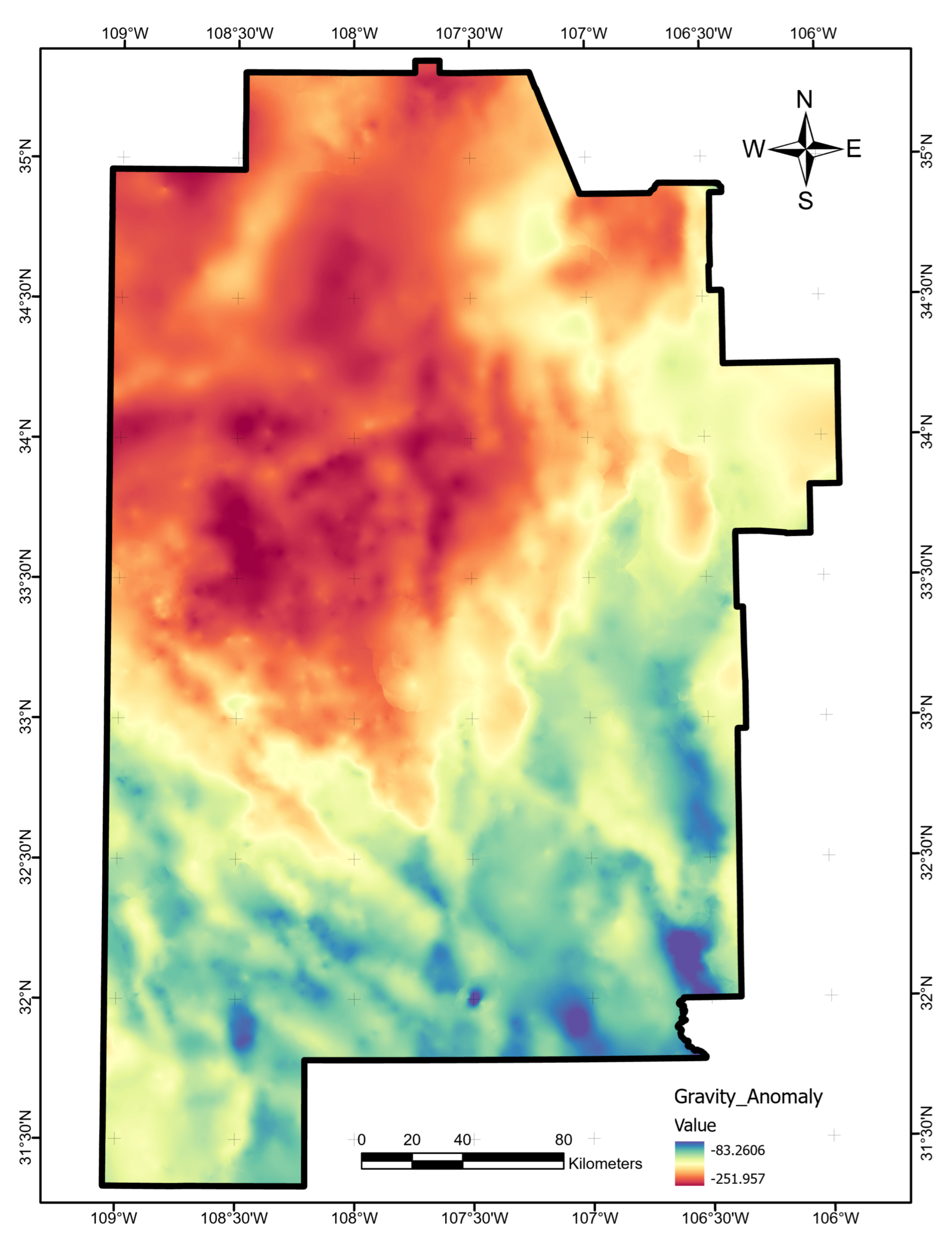
Appendix A.10. Gravity Anomaly
We obtained terrain-corrected gravity-anomaly data available from the University of Texas El Paso [26] directly from the original southwest New Mexico PFA submission to the OpenEI repository [17]. This layer required no further processing (Figure A10).
Figure A10.
Gravity-anomaly data layer map, produced using ArcGIS Pro. Units are milligals (mGal). Raster obtained from OpenEI archive [17].
Figure A10.
Gravity-anomaly data layer map, produced using ArcGIS Pro. Units are milligals (mGal). Raster obtained from OpenEI archive [17].

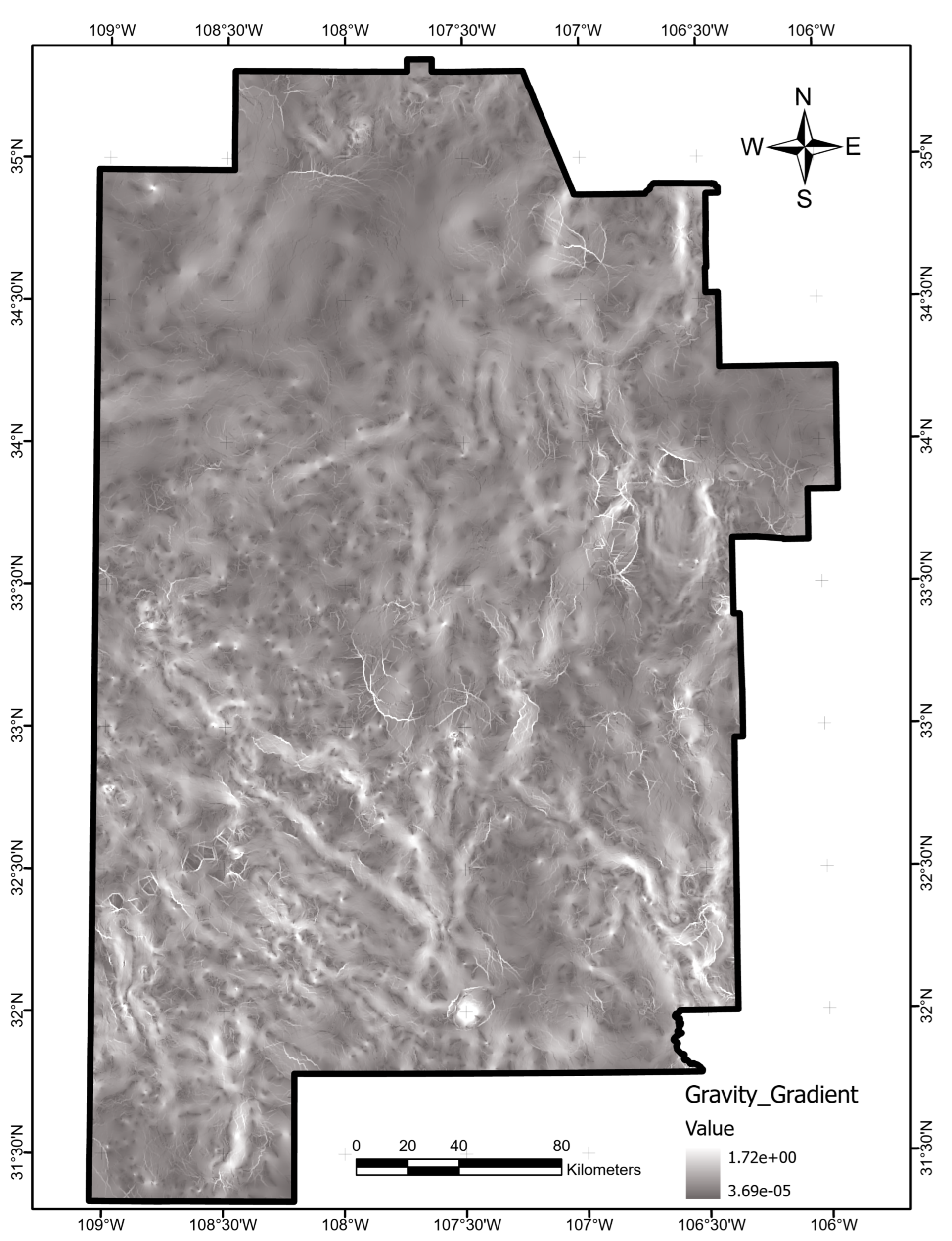
Appendix A.11. Gravity-Anomaly Gradient
Gravity-anomaly gradient values were calculated by taking the slope of the gravity-anomaly layer. Figure A11 shows the final data layer, calculated as slope degrees or where mGal/m is a reference gradient of the gravity anomaly .
Figure A11.
Gravity-anomaly gradient data layer map, produced using ArcGIS Pro. Units are degrees.

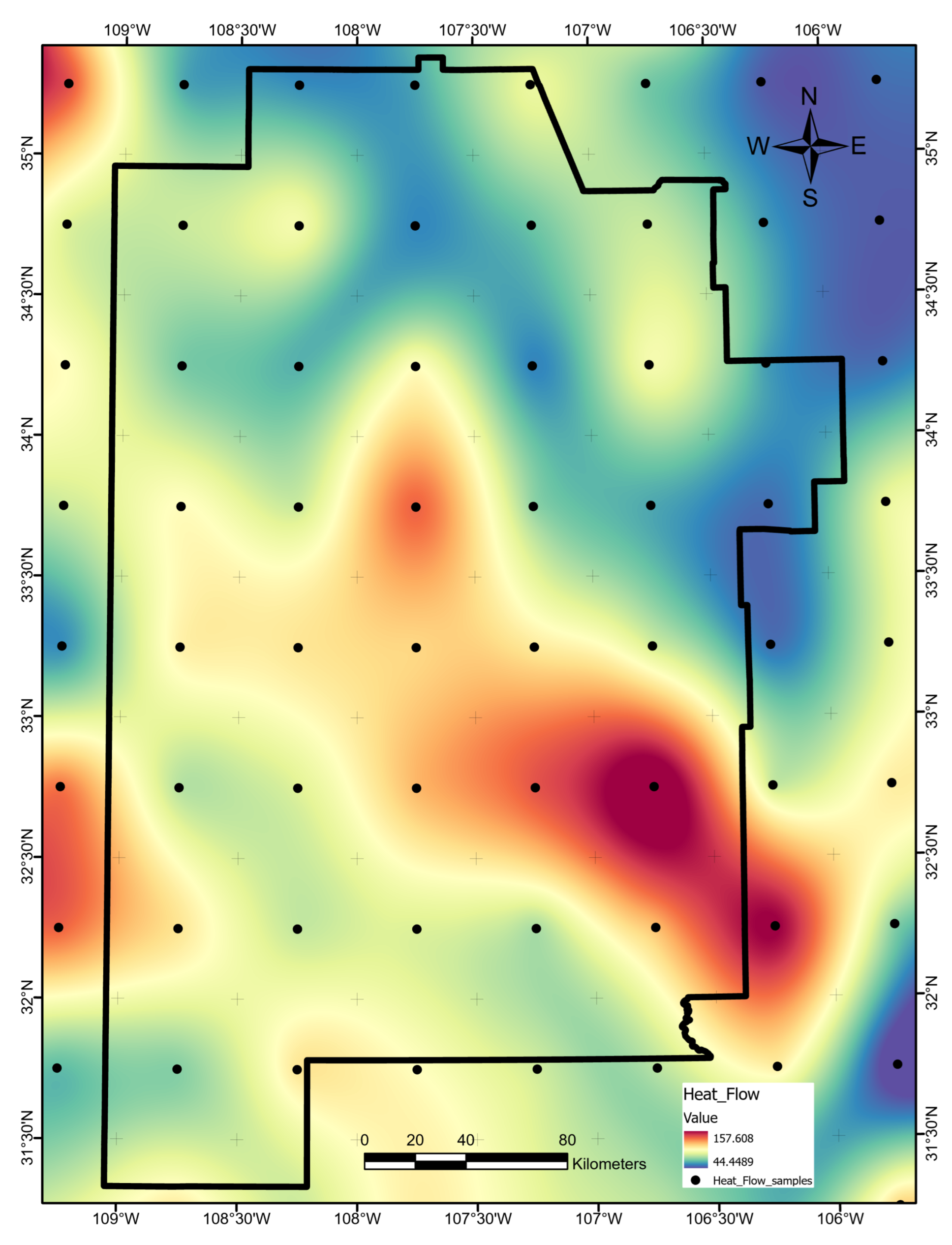
Appendix A.12. Heat Flow
The -resolution heat-flow model from Lucazeau [27] offers coarse coverage across the southwest NM study area. We obtained the data from the supporting information section of the publication web-page [27]. Then, we interpolated with the ArcGIS Topo to Raster function, which uses an iterative finite difference method and removes local minima not supported by the input data [66] to generate the final data layer (Figure A12).
Figure A12.
Heat-flow data layer map, produced using ArcGIS Pro. Units are mW m. Black dots mark the original source data points from Lucazeau [27].
Figure A12.
Heat-flow data layer map, produced using ArcGIS Pro. Units are mW m. Black dots mark the original source data points from Lucazeau [27].

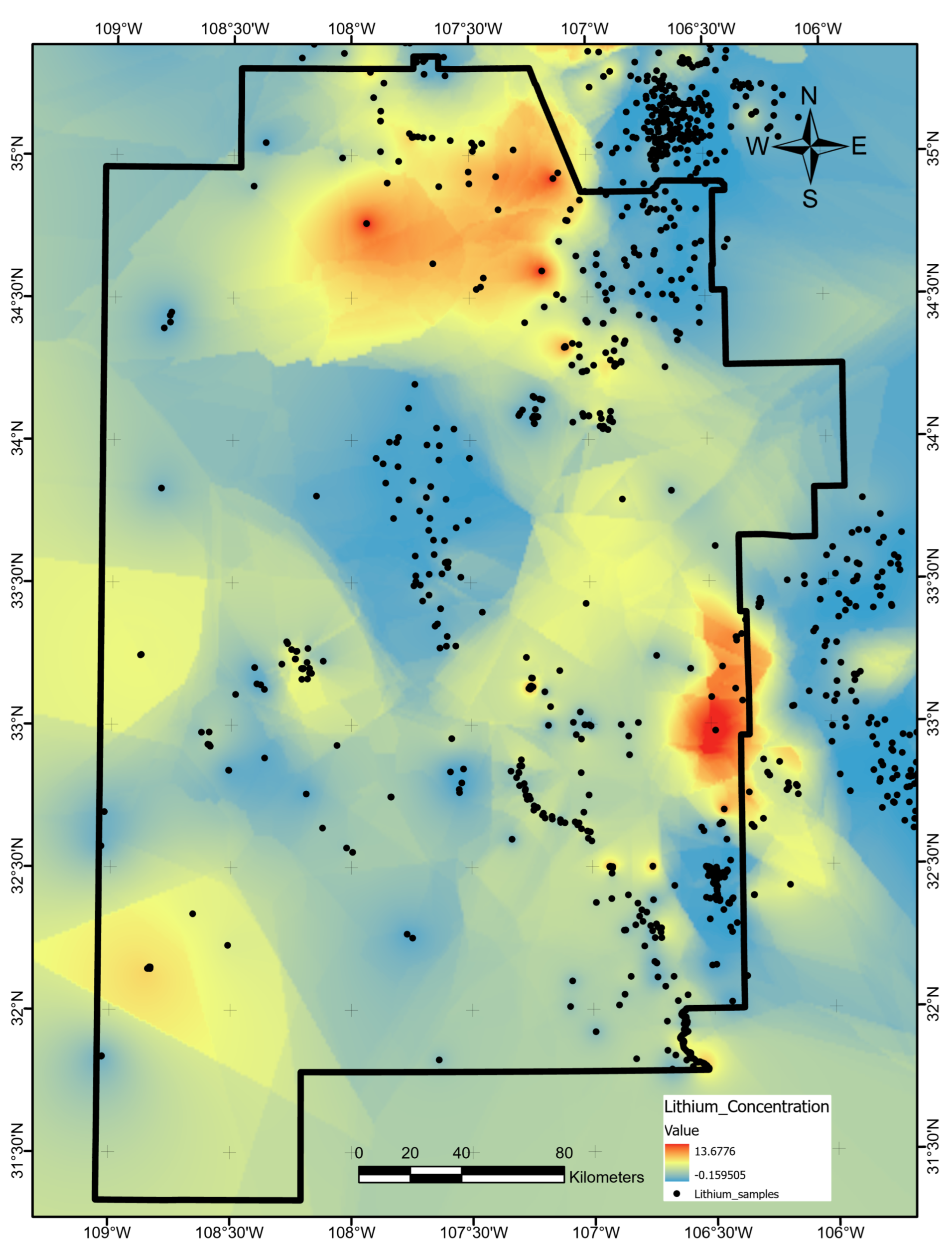
Appendix A.13. Lithium Concentration
Measurements of lithium concentration were collected by Bielicki et al. [16] from USGS records, student dissertations, and other sources. After retrieving these point data from the OpenEI archive [17], we interpolated 3595 measurements in the study region using EBK as described for the boron layer. Figure A13 shows the final results. Note that kriging solutions such as this may show ridge-like edges and boundaries between patches of the interpolated surface by nature of the kriging algorithm [65].

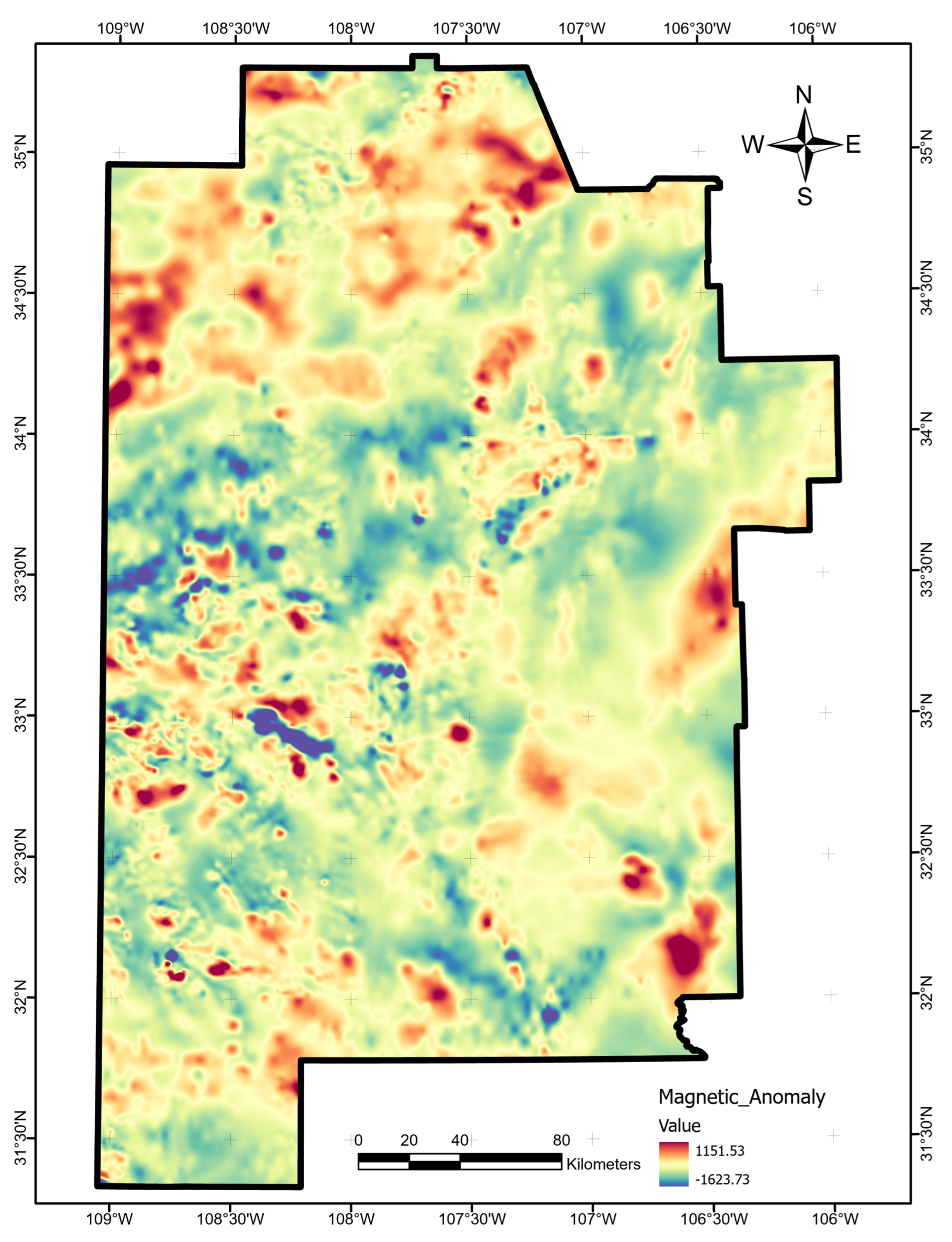
Appendix A.14. Magnetic Anomaly
We obtained USGS magnetic-anomaly based on aerial surveys [70] directly from the original southwest New Mexico PFA submission to the OpenEI repository [17]. This layer required no further processing (Figure A14).
Figure A14.
Magnetic-anomaly data layer map, produced using ArcGIS Pro. Units are nanoteslas. Raster obtained from OpenEI archive [17].
Figure A14.
Magnetic-anomaly data layer map, produced using ArcGIS Pro. Units are nanoteslas. Raster obtained from OpenEI archive [17].

Appendix A.15. Magnetic-Anomaly Gradient
Magnetic-anomaly gradient values were calculated by taking the slope of the magnetic-anomaly layer. Figure A15 shows the final data layer, which is calculated as slope degrees or where nT/m is the reference gradient of the magnetic anomaly .
Figure A15.
Magnetic-anomaly gradient data layer map, produced using ArcGIS Pro. Units are degrees.

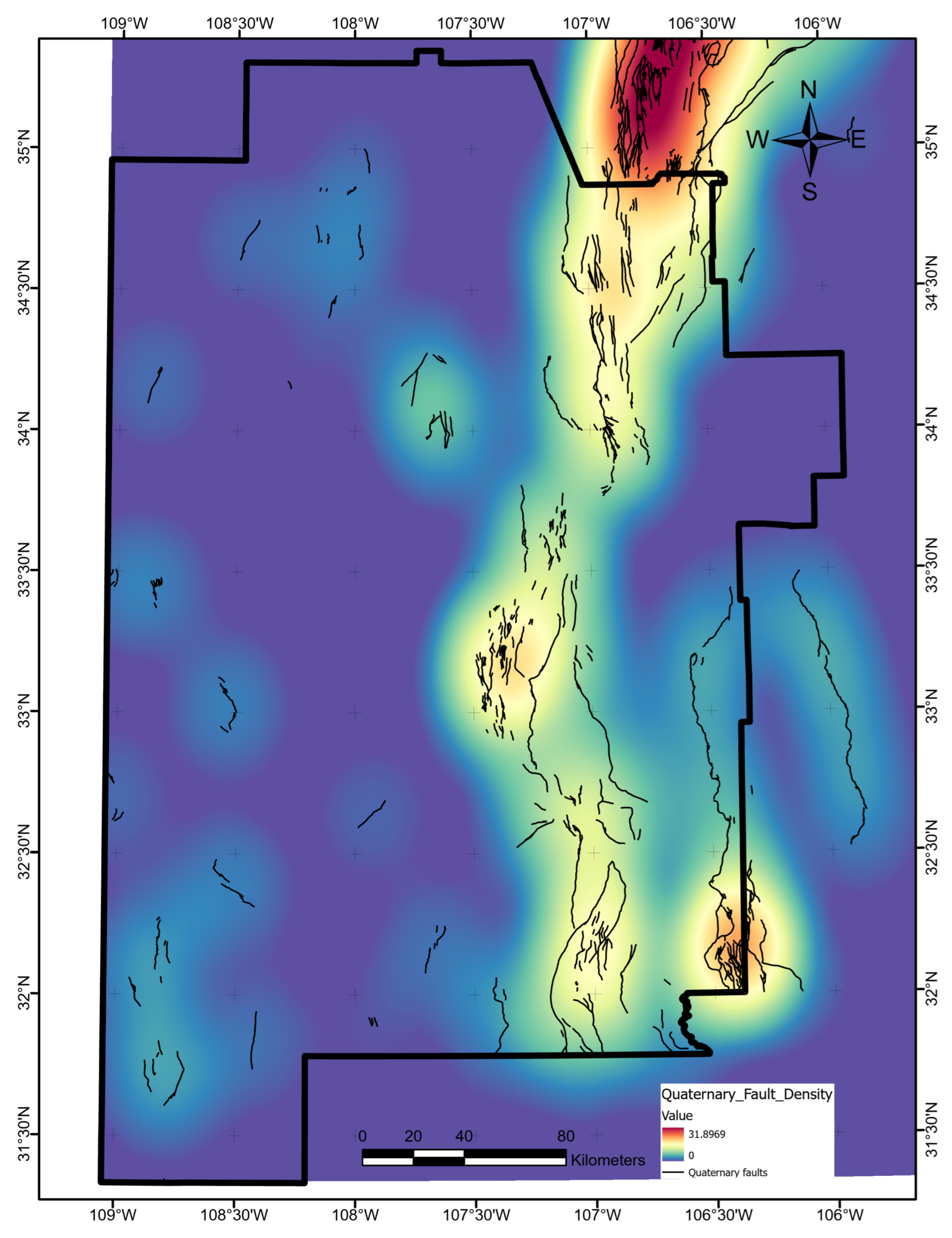
Appendix A.16. Quaternary Fault Density
Faults showing Quaternary displacement were originally digitized at the 1:24,000 scale by the New Mexico Bureau of Geology and Mineral Resources and provided to Bielicki et al. [16]. We obtained the associated polylines from the OpenEI PFA submission [17] and then applied the same line-based kernel density estimate used for the drainage density layer, with a decay radius of . Figure A16 shows the final data layer.

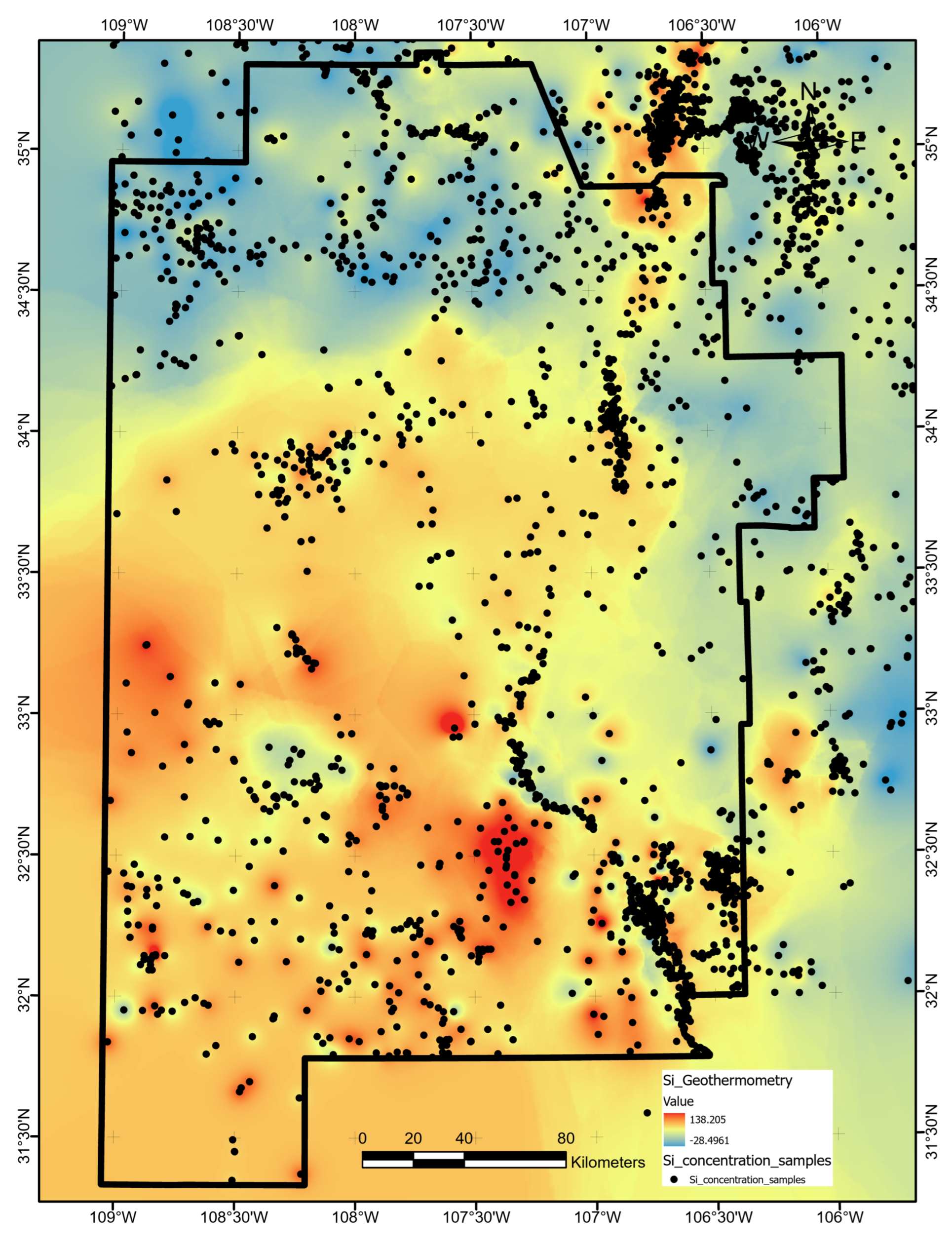
Appendix A.17. Silica Geothermometer Temperature
Silica-concentration data were compiled by Bielicki et al. [16] and converted to reservoir temperatures using the Fournier chalcedony geothermometer relationship [71]. After retrieving the point data from OpenEI [17], we interpolated the 7259 measurements using EBK as described for the boron layer. Figure A17 shows the final results.
Figure A17.
Chalcedony geothermometer data layer map, produced using ArcGIS Pro. Units are C. Black dots indicate locations where silica concentration was sampled, as collected by Bielicki et al. [16,17].

Note that low groundwater silica concentrations can lead to physically unrealistic negative temperatures with the Fournier relationship. These values are preserved to capture relative variation in silica concentrations. The ML methods only focus on relative variations the scaled and transformed data, not absolute magnitudes, so negative Si geothermometer temperatures can be tolerated.
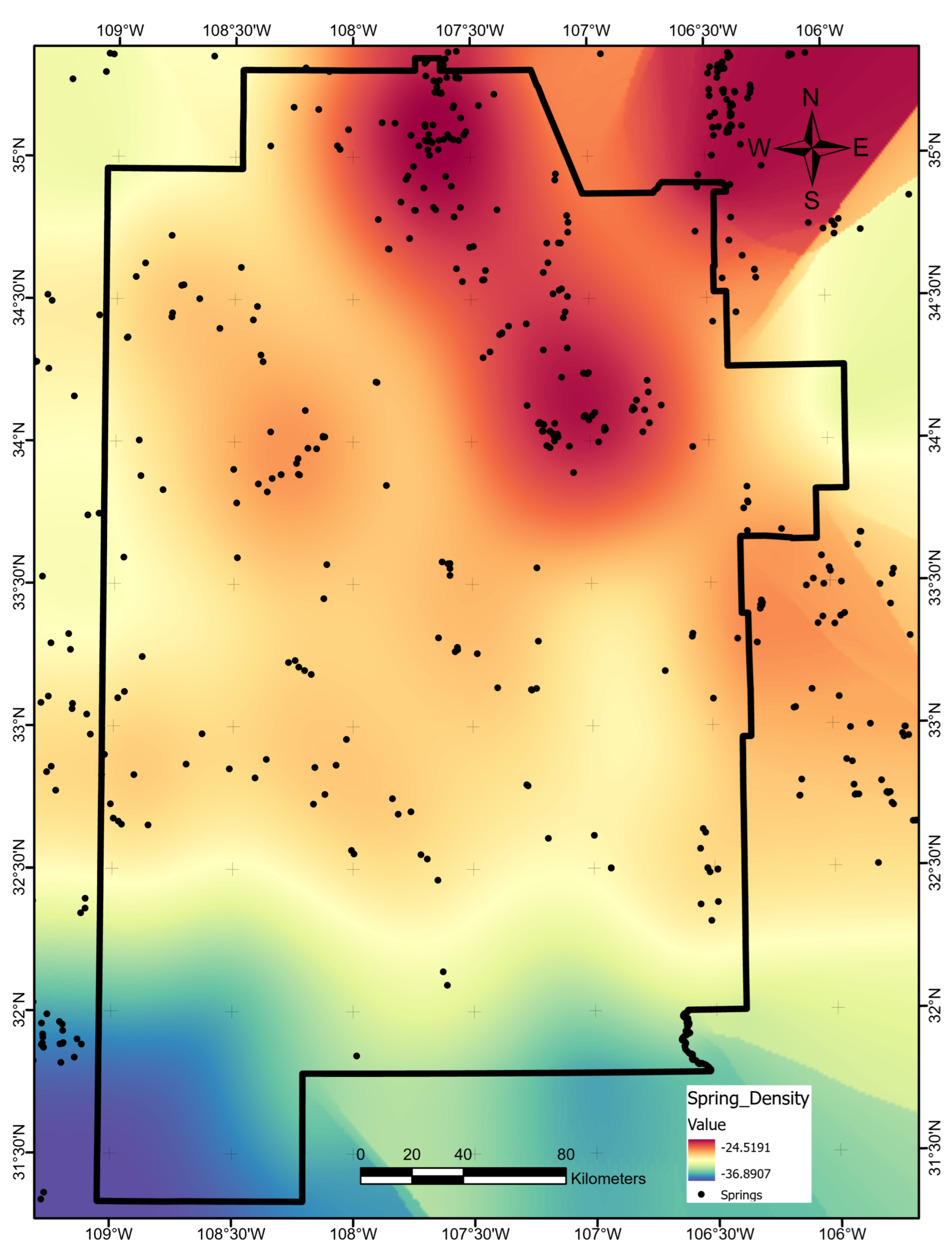
Appendix A.18. Spring Density
We obtained 2565 locations of springs within the study region from the USGS National Water Information System [28]. As with the earthquake density layer, we used a grid search routine with 10-fold cross-validation to determine the best search radius of 31,400 m for a spring KDE. The resulting data layer is shown in Figure A18.
Figure A18.
Natural logarithm of spring density in number per km. Map produced using ArcGIS Pro. Black dots indicate spring locations from the USGS [28].
Figure A18.
Natural logarithm of spring density in number per km. Map produced using ArcGIS Pro. Black dots indicate spring locations from the USGS [28].

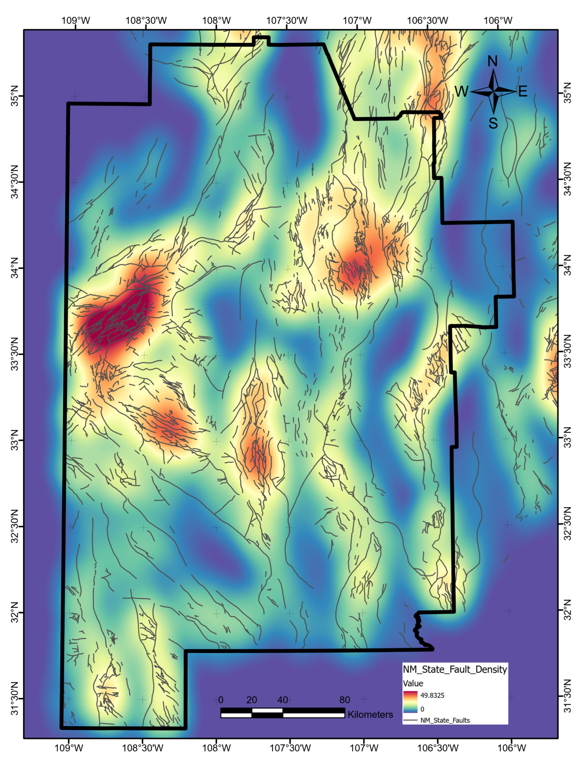
Appendix A.19. State Map Fault Density
We retrieved New Mexico state fault outlines from the USGS Energy and Environment in the Rocky Mountain Area data portal [30,72]. As with the Quaternary fault layer, we converted the polylines to fault density using line-based KDE with a radius of . Figure A19 shows the final data layer.
Figure A19.
State fault-density data layer map, produced using ArcGIS Pro. Units are degree/degree. Dark gray lines trace the fault polyline data set obtained from USGS Open-File Report 2005-1351 [72].
Figure A19.
State fault-density data layer map, produced using ArcGIS Pro. Units are degree/degree. Dark gray lines trace the fault polyline data set obtained from USGS Open-File Report 2005-1351 [72].

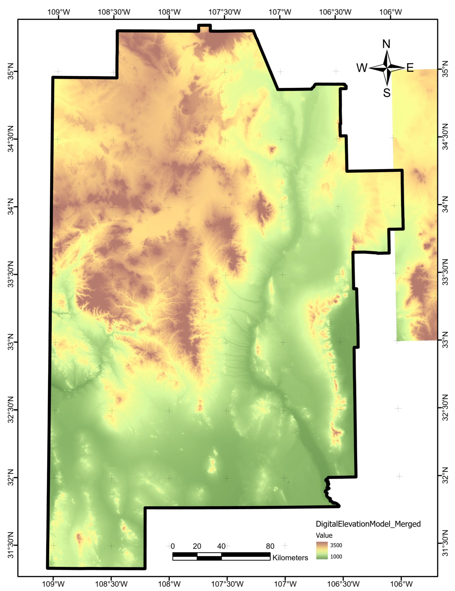
Appendix A.20. Surface Topography (DEM)
We obtained a Digital Elevation Model (DEM) raster with surface topography at one arc-sec resolution from the southwest New Mexico PFA OpenEI archive [17]. To address a data gap to the east, we merged in two DEM tiles at the same resolution from the USGS National Map website [29]. The final data layer required no further processing (Figure A20).

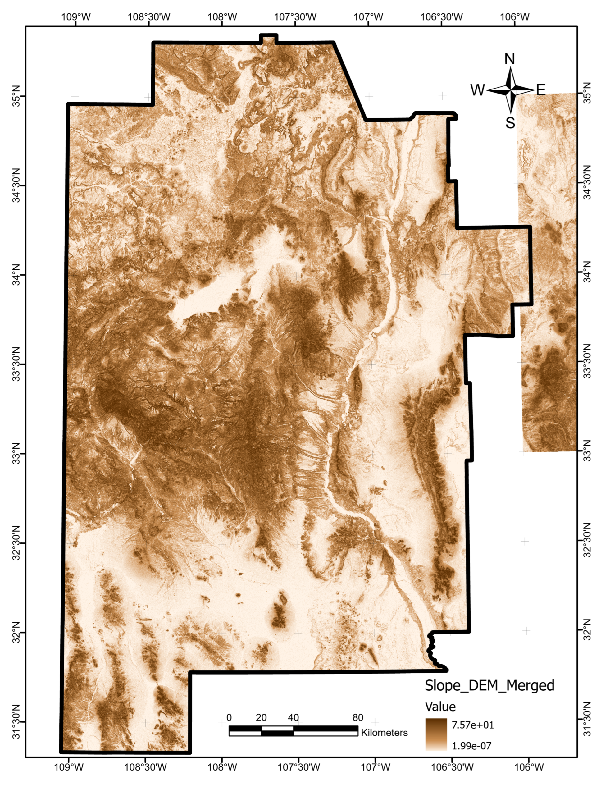
Appendix A.21. Topographic Gradient
We calculated topographic-gradient magnitude by taking the slope of the DEM raster as was performed for both gravity-anomaly and magnetic-anomaly gradient. Figure A21 shows the final data layer in slope degrees.
Figure A21.
Topographic gradient data layer map, produced using ArcGIS Pro. Units are degrees.

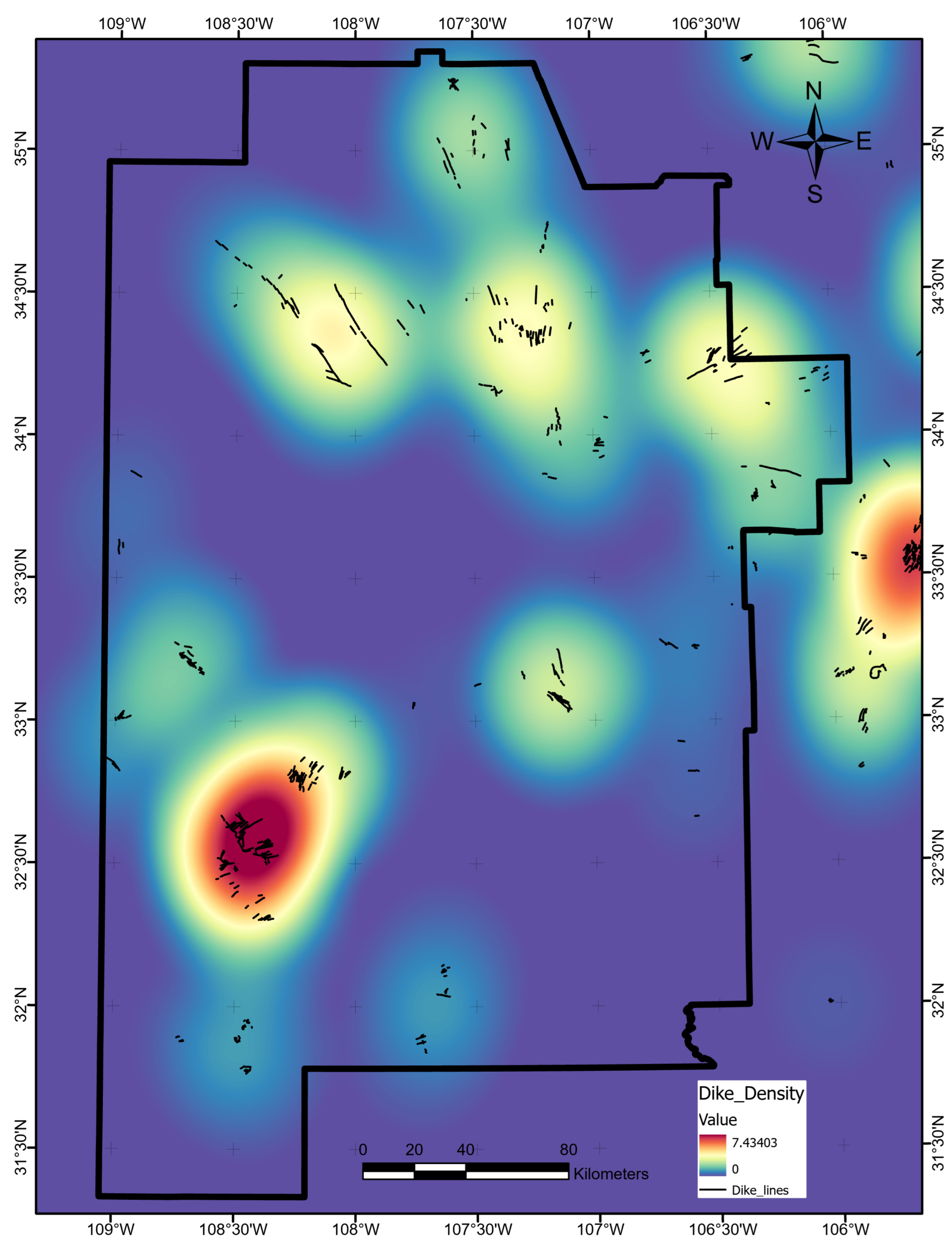
Appendix A.22. Volcanic-Dike Density
We retrieved digitized volcanic-dike outlines from the USGS Energy and Environment in the Rocky Mountain Area data portal [30,72]. As with the Quaternary fault layer, we converted the polylines to dike density using line-based KDE with a radius of . Figure A22 shows the final data layer.
Figure A22.
Volcanic dike-density data layer map, produced using ArcGIS Pro. Units are in degree/degree. Black lines trace the dike polyline data set obtained from USGS Open-File Report 2005-1351 [72].
Figure A22.
Volcanic dike-density data layer map, produced using ArcGIS Pro. Units are in degree/degree. Black lines trace the dike polyline data set obtained from USGS Open-File Report 2005-1351 [72].

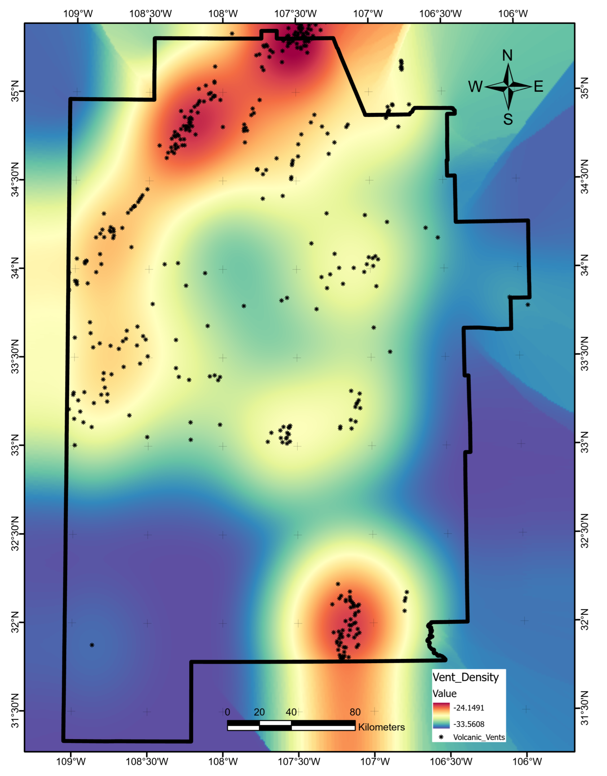
Appendix A.23. Volcanic-Vent Density
We obtained 811 volcanic vent locations within the study area from the New Mexico Bureau of Geology and Mineral Resources using the NMBGMR Interactive Map [73]. As with the earthquake density layer, we used a grid search routine with 10-fold cross-validation to determine the best search radius of 28,300 m for a volcanic vent KDE. The final data layer is shown in Figure A23.
Figure A23.
Natural logarithm of vent density in number per km. Map produced using ArcGIS Pro. Black dots indicate vent locations from the NMBGMR [73].
Figure A23.
Natural logarithm of vent density in number per km. Map produced using ArcGIS Pro. Black dots indicate vent locations from the NMBGMR [73].

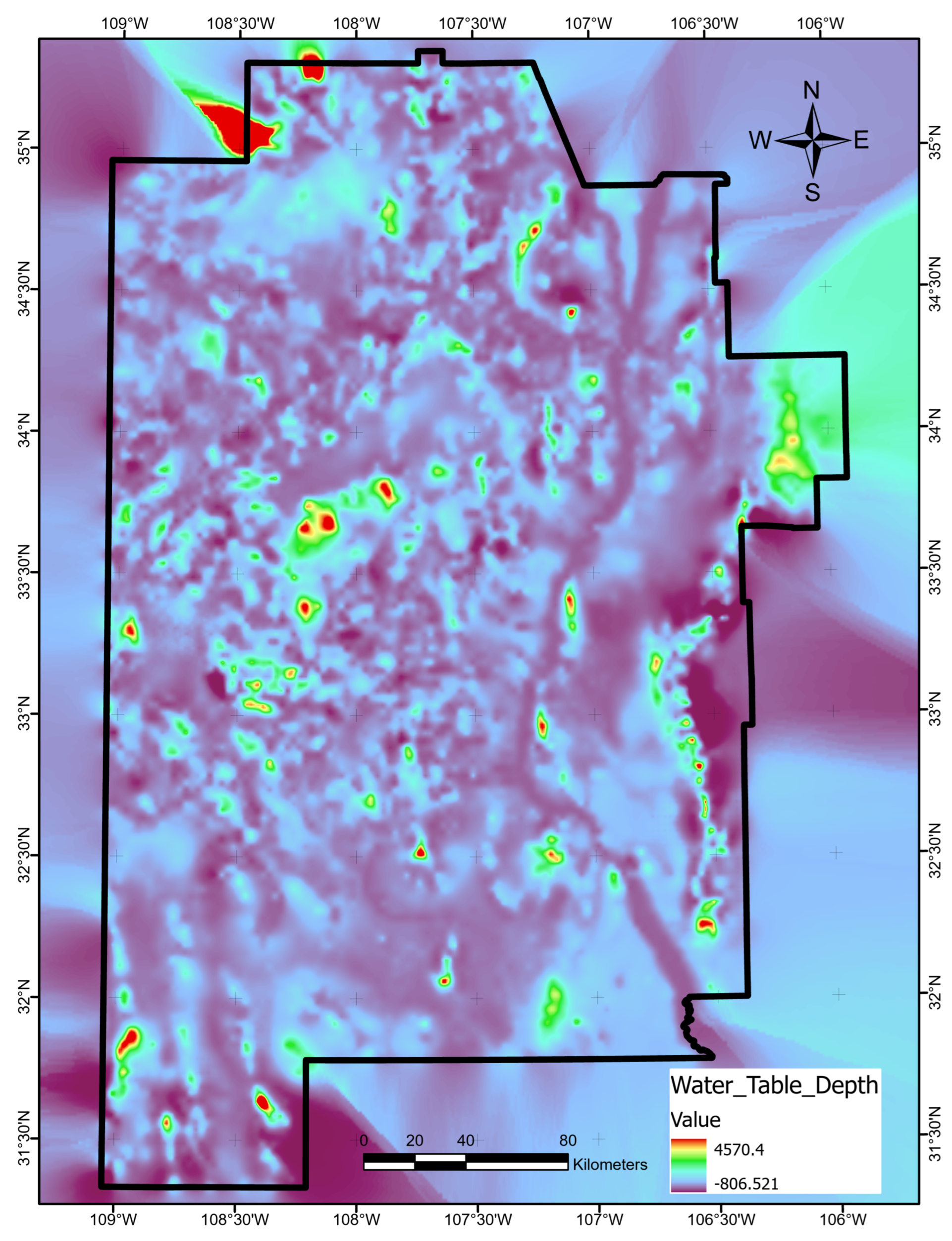
Appendix A.24. Water-Table Depth
We obtained a depth to water table raster constructed by Bielicki et al. [16] from the southwest New Mexico PFA archive [17]. Data gaps to the south and east of the study area were filled using empirical Bayes kriging [61] with exponential semivariograms and a maximum of 100 points in 100 simulations. Figure A24 illustrates the final result.

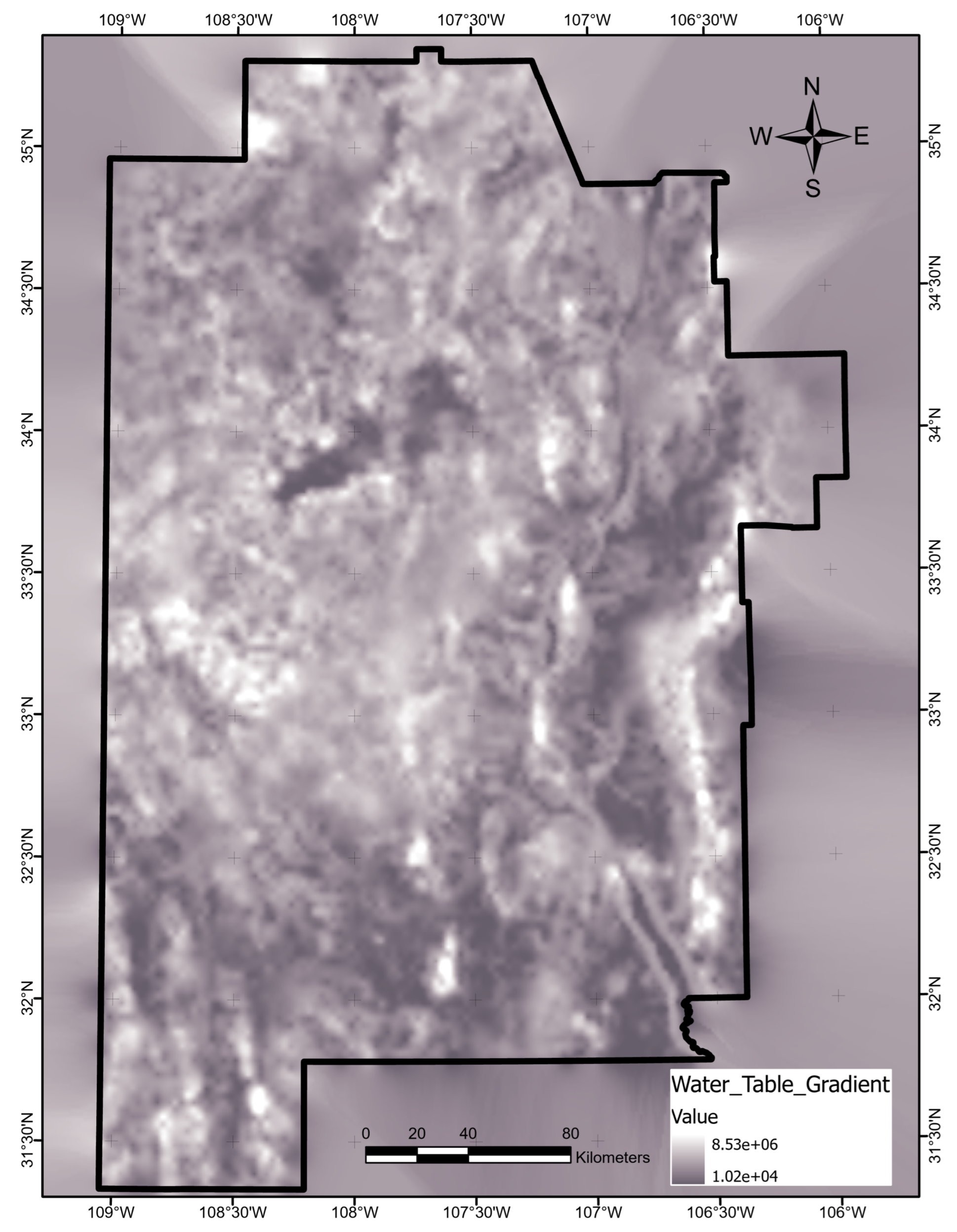
Appendix A.25. Water-Table Gradient
We retrieved a raster of the water-table gradient from the southwest New Mexico PFA archive [17]. As with the water-table depth data layer, gaps to the south and east of the study area were filled using EBK [61] with exponential semivariograms and a maximum of 100 points in 100 simulations. Figure A25 illustrates the final result.

Appendix A.26. Geothermal Gradient
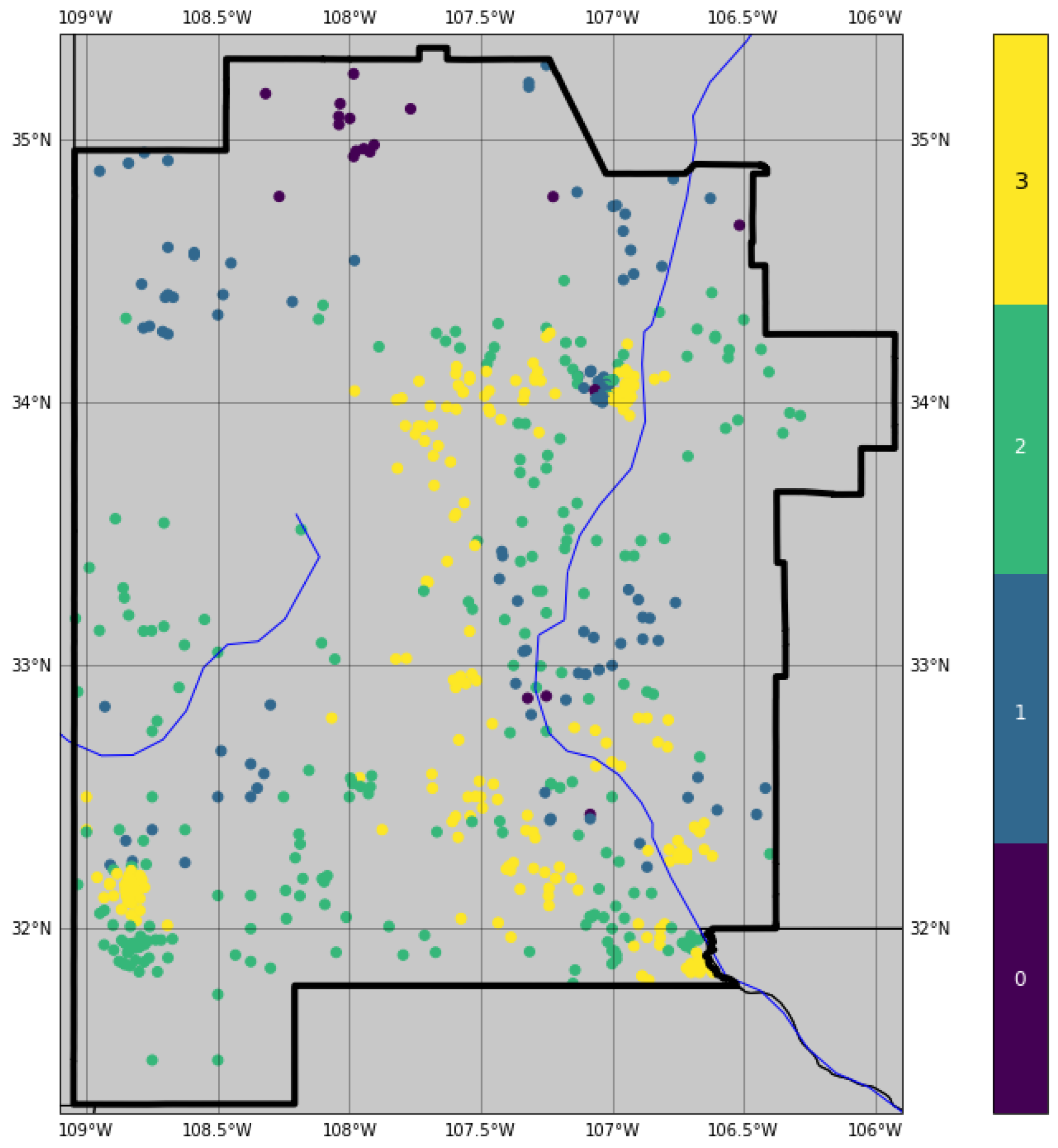
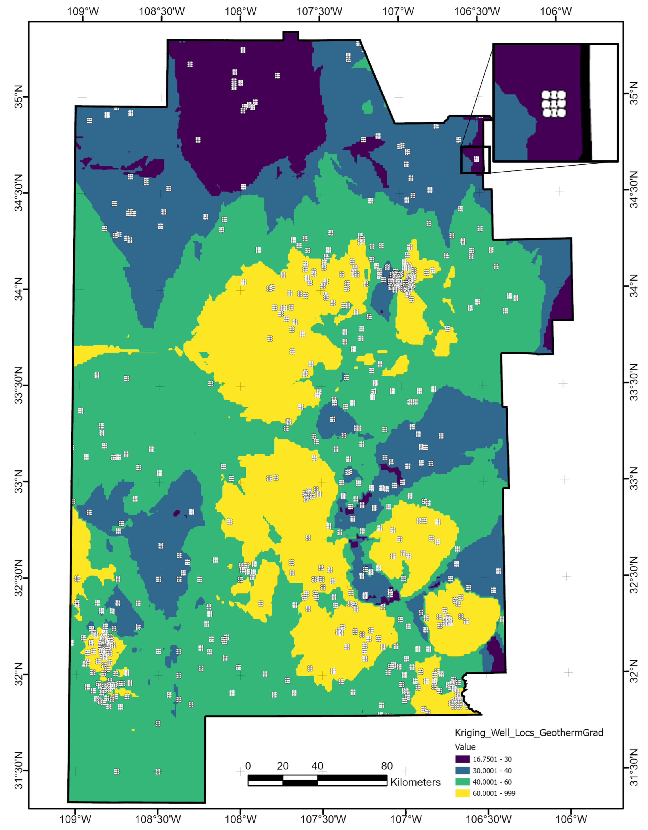
The SMU Heat Flow Database from BHT Data catalog contains geothermal gradient values in two forms: reported gradient and corrected gradient [31]. We selected the corrected geothermal gradient when available, and we used the uncorrected value otherwise. For the 20% of well locations with multiple geothermal gradient measurements, often recorded for different intervals within a well, we chose the highest value assuming that interval would be the target for any enthalpy capture. Three negative geothermal gradient records were discarded due to lack of information to verify the anomalous values. Figure A26 depicts the final set of 596 values in the study area after binning into the geothermal-gradient classes described in Table 2. Figure A27 shows the results of kriging the well data in Figure A26 for assigning geothermal-gradient values during the data-augmentation step. Additionally shown are the wells and pseudowells of the WDS8 data set. Keeping the step-out distance short () reduces the imprint of the kriging result on the augmented data sets, and kriging adds consistency to overlapping pseudowells in areas where well density is high.
Figure A26.
Geothermal-gradient observations from well data. Markers are colored by geothermal-gradient class. Data were retrieved from the SMU NGDS portal [31].
Figure A26.
Geothermal-gradient observations from well data. Markers are colored by geothermal-gradient class. Data were retrieved from the SMU NGDS portal [31].

Figure A27.
Geothermal gradient based on kriging of WDS data set used for data augmentation. Map produced using ArcGIS Pro. The layer consists of continuous values in K/km interpolated for the geothermal gradient, visualized using color binning to simulate classification label assignments. White markers depict the WDS8 wells and pseudowells. Inset map shows zoomed-in view to illustrate the short step-out of the pseudowells from the original WDS well locations.

Appendix B. Methods Supplementary Information
Appendix B.1. Data Scaling and Transformation
We applied the Z-score formulation for standardizing feature data prior to modeling. This method resets the statistical moments of a feature to zero mean and unit variance:
where and are the sample mean and variance of x.
We paired data scaling with non-linear data transformations to replace feature distribution skewness with more Gaussian-like symmetry. Specifically, the data underwent a Yeo–Johnson power transformation, which uses a parameter, , to select from among a family of transformations [37]:
Appendix B.2. Hyperparameter Tuning
We pursued a k-Fold cross-validation (CV) approach to hyperparameter tuning given the small size of our data sets. Training data were split into k (typically 5 or 10) folds, and the model was repeatedly trained on the aggregate of all but one fold; then, it was scored using the predictions on the remaining fold [47]. This strategy cycled through all k permutations of splitting the data, and the scores were averaged to create a summary statistic (AUC). We used a stratified-sampled strategy to define the folds such that class proportions of the unpartitioned data are preserved within each fold.
During tuning, the k-fold CV process defined average scores for all hyperparameter values under consideration. In some cases, a clear maximum in the results indicated the best value to use. In others, the scores level off to form a corner or “elbow” in a parameter value AUC plot. Choosing a hyperparameter value near this corner position balances the trade-off between overfitting and underfitting the training data. We include all tuning steps and hyperparameter plots in the code repository for this study [34].
Appendix B.3. Model Hyperparameters
The following tables describe the final hyperparameter choices determined from the tuning process for all three data sets in the study.
Appendix B.3.1. Logistic Regression
The scikit-learn logistic regression classifier used in this analysis includes a single tunable hyperparameter, , that acts as a regularization term [45]. The chosen values are listed in Table A1.

Table A1.
Logistic regression hyperparameter tuning results for each data set.
| WDS | WDS4 | WDS8 | |
|---|---|---|---|
| C | 0.110 | 0.085 | 0.050 |
Appendix B.3.2. Decision Tree Classifier
We tuned six hyperparameters for the scikit-learn decision tree classifier: and together, followed by , , , and . The chosen hyperparameter values are listed in Table A2.
Table A2.
Decision tree hyperparameter tuning results for each data set.
| WDS | WDS4 | WDS8 | |
|---|---|---|---|
| criterion | Gini | Entropy | Entropy |
| max_depth | 5 | 9 | 10 |
| min_samples_leaf | 7 | 7 | 8 |
| min_samples_split | 21 | 18 | 23 |
| max_features | 17 | 20 | 17 |
| ccp_alpha | 0.02 | 0.01 | 0.005 |
Appendix B.3.3. XGBoost Classifier
When tuning the XGBoost classifier, we considered nine hyperparameters in succession: , , , ,, , , , and . We adjusted the last two together to balance quality of fit with risk of overfitting. Final hyperparameter choices are provided in Table A3.
Table A3.
XGBoost hyperparameter tuning results for each data set.
| WDS | WDS4 | WDS8 | |
|---|---|---|---|
| max_depth | 5 | 5 | 4 |
| min_child_weight | 7 | 3 | 3 |
| gamma | 0.1 | 0.1 | 0.2 |
| subsample | 0.5 | 0.6 | 0.5 |
| colsample_bytree | 0.6 | 0.5 | 0.5 |
| reg_lambda | 1.27 | 1.27 | 1.27 |
| scale_pos_weight | 0.0 | 0.0 | 0.0 |
| learning_rate | 0.005 | 0.005 | 0.005 |
| n_estimators | 1000 | 1000 | 1750 |
Appendix B.3.4. Artificial Neural Network Classifier
In addition to defining the architecture for the TensorFlow ANN shown in Figure A28, we tuned five hyperparameters: , , , , and . The final selected hyperparameter values are provided in Table A4.
Table A4.
Artificial neural network hyperparameter tuning results for each data set.
| WDS | WDS4 | WDS8 | |
|---|---|---|---|
| learning rate | 0.001 | 0.010 | 0.010 |
| lambda | |||
| batch size | 20 | 45 | 100 |
| dropout rate | 0.1 | 0.1 | 0.1 |
| epochs | 75 | 200 | 300 |
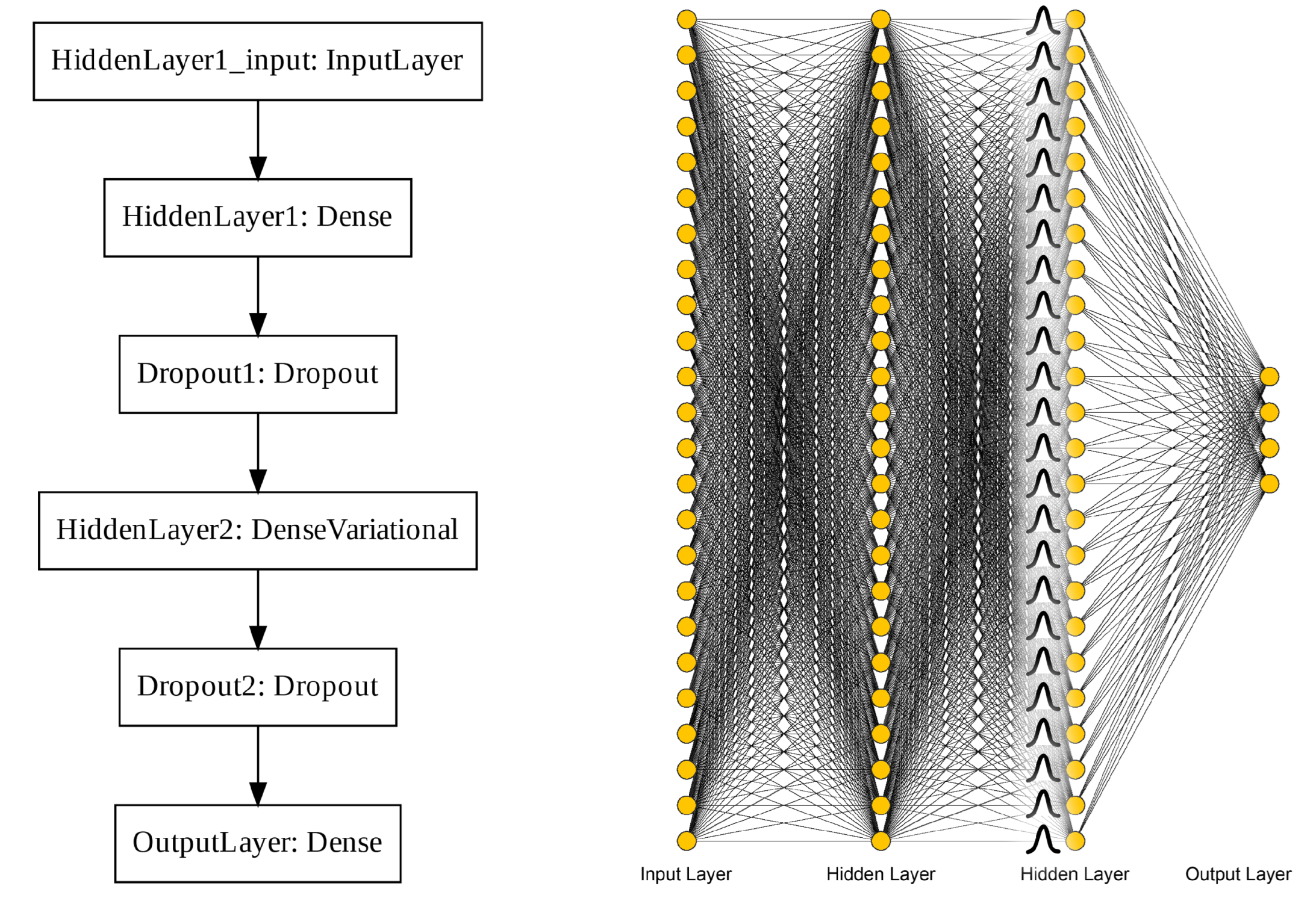
The BNN constructed for Section 2.4.2 follows the same architectural pattern as the ANN, but it replaces one Tensorflow Dense layer with a Tensorflow Probability DenseVariational layer [51,60]. Figure A29 shows a simplified diagram illustrating where deterministic weights are replaced by distribution functions in the second hidden layer. The ANN hyperparameters listed in Table A4 were similarly applied to the BNN to support a direct analogy between the two in the analysis.
Figure A28.
Tensorflow output and diagrammatic depictions of the ANN fully-connected four-layer architecture [51]. The input layer takes values from the 24 features as inputs, which feed forward through two hidden layers to the output layer for a four-class classification.
Figure A28.
Tensorflow output and diagrammatic depictions of the ANN fully-connected four-layer architecture [51]. The input layer takes values from the 24 features as inputs, which feed forward through two hidden layers to the output layer for a four-class classification.

Figure A29.
Tensorflow output and diagrammatic depictions of the BNN fully-connected four-layer architecture. The difference between this and the ANN in Figure A28 is the replacement of HiddenLayer2 with a probabilistic layer.
Figure A29.
Tensorflow output and diagrammatic depictions of the BNN fully-connected four-layer architecture. The difference between this and the ANN in Figure A28 is the replacement of HiddenLayer2 with a probabilistic layer.

References
- Glassley, W.E. Geothermal Energy: Renewable Energy and the Environment, 2nd ed.; CRC Press: Boca Raton, FL, USA, 2015; pp. 123–125. [Google Scholar]
- Garchar, L.; Badgett, A.; Nieto, A.; Young, K.; Hass, E.; Weathers, M. Geothermal play fairway analysis: Phase I summary. In Proceedings of the Fortieth Workshop on Geothermal Reservoir Engineering, Stanford, CA, USA, 22–24 February 2016. [Google Scholar]
- Doust, H. The exploration play: What do we mean by it? AAPG Bull. 2010, 94, 1657–1672. [Google Scholar] [CrossRef]
- Lottaroli, F.; Craig, J.; Cozzi, A. Evaluating a vintage play fairway exercise using subsequent exploration results: Did it work? Pet. Geosci. 2018, 24, 159–171. [Google Scholar] [CrossRef]
- Faulds, J.; Craig, J.; Coolbaugh, M.; Hinz, N.; Glen, J.; Deoreo, S. Searching for blind geothermal systems utilizing play fairway analysis, western Nevada. GRC Bull. 2018, 47, EE0006731. [Google Scholar]
- Wannamaker, P.E.; Meigs, A.J.; Trimble, J.D.; Lamont, E.A.; Kennedy, B.M.; Moore, J.N.; Maris, V.; Sonnenthal, E.L.; Nash, G.D. Play fairway analysis for structurally controlled geothermal systems in the Central Cascades arc-backarc regime, Oregon. In Proceedings of the 41st Workshop on Geothermal Reservoir Engineering Stanford University, Stanford, CA, USA, 22–24 February 2016; Volume 22, p. 24. [Google Scholar]
- Jordan, T.E.; Richards, M.C.; Horowitz, F.G.; Camp, E.; Smith, J.D.; Whealton, C.A.; Stedinger, J.R.; Hornbach, M.J.; Frone, Z.S.; Tester, J.W. Low Temperature Geothermal Play Fairway Analysis for the Appalachian Basin: Phase 1 Revised Report November 18, 2016; Technical Report; Cornell University: Ithaca, NY, USA, 2016. [Google Scholar]
- Gunderson, K.L.; Holmes, R.C.; Loisel, J. Recent digital technology trends in geoscience teaching and practice. GSA Today 2020, 30. [Google Scholar] [CrossRef]
- Pepin, J. New Approaches to Geothermal Resource Exploration and Characterization. Ph.D. Thesis, New Mexico Institute of Mining and Technology, Socorro, NM, USA, 2019. [Google Scholar]
- Siler, D.L.; Pepin, J.D.; Vesselinov, V.V.; Mudunuru, M.K.; Ahmmed, B. Machine learning to identify geologic factors associated with production in geothermal fields: A case-study using 3D geologic data, Brady geothermal field, Nevada. Geotherm. Energy 2021, 9, 17. [Google Scholar] [CrossRef]
- Smith, C.M.; Faulds, J.E.; Brown, S.; Coolbaugh, M.; Lindsey, C.R.; Treitel, S.; Ayling, B.; Fehler, M.; Gu, C.; Mlawsky, E. Characterizing Signatures of Geothermal Exploration Data with Machine Learning Techniques: An Application to the Nevada Play Fairway Analysis. In Proceedings of the 46th Workshop on Geothermal Reservoir Engineering, Stanford, CA, USA, 16–18 February 2021. [Google Scholar]
- Brown, S.C.; Coolbaugh, M.F.; DeAngelo, J.; Faulds, J.E.; Fehler, M.; Gu, C.; Queen, J.H.; Treitel, S.; Smith, C.M.; Mlawsky, E. Machine learning for natural resource assessment: An application to the blind geothermal systems of Nevada. Geotherm. Resour. Counc. Trans. 2020, 44, 13. [Google Scholar]
- Rezvanbehbahani, S.; Stearns, L.A.; Kadivar, A.; Walker, J.D.; van der Veen, C.J. Predicting the Geothermal Heat Flux in Greenland: A Machine Learning Approach. Geophys. Res. Lett. 2017, 44, 12271–12279. [Google Scholar] [CrossRef] [Green Version]
- Shahdi, A.; Lee, S.; Karpatne, A.; Nojabaei, B. Exploratory analysis of machine learning methods in predicting subsurface temperature and geothermal gradient of Northeastern United States. Geotherm. Energy 2021, 9, 18. [Google Scholar] [CrossRef]
- Witter, J.B.; Trainor-Guitton, W.J.; Siler, D.L. Uncertainty and risk evaluation during the exploration stage of geothermal development: A review. Geothermics 2019, 78, 233–242. [Google Scholar] [CrossRef]
- Bielicki, J.; Blackwell, D.; Harp, D.; Karra, S.; Kelley, R.; Kelly, S.; Middleton, R.; Pepin, J.; Person, M.; Sutula, G. Hydrogeolgic Windows: Regional Signature Detection for Blind and Traditional Geothermal Play Fairways, Final Reports, Los Alamos National Laboratory; Technical Report, LA-UR-15-28360; Los Alamos National Laboratory: Los Alamos, NM, USA, 2015. [Google Scholar]
- Los Alamos National Laboratory. New Mexico Geothermal Play Fairway Analysis from LANL; Los Alamos National Laboratory: Los Alamos, NM, USA, 2015. [Google Scholar] [CrossRef]
- PRISM. PRISM Climate Group, Oregon State U. 2021. Available online: https://prism.oregonstate.edu/normals/ (accessed on 6 February 2021).
- Keller, G.R.; Khan, A.; Morganc, P.; Wendlandt, R.; Baldridge, S.; Olsen, K.; Prodehl, C.; Braile, L.W. A comparative study of the Rio Grande and Kenya rifts. Tectonophysics 1991, 197, 355–371. [Google Scholar] [CrossRef]
- Sanford, A.; Lin, K.W.; Tsai, I.C.; Jaksha, L.H. Earthquake catalogs for New Mexico and bordering areas: 1869–1998. New Mex. Bur. Geol. Miner. Resour. Circ. 2002, 210, 1–9. [Google Scholar]
- Sanford, A. Earthquake catalogs for New Mexico and bordering areas II: 1999–2004. New Mex. Geol. 2006, 28, 99–109. [Google Scholar]
- Pursley, J. Earthquake catalogs for New Mexico and bordering areas: 2005–2009. New Mex. Geol. 2013, 35, 3–12. [Google Scholar]
- USGS. Earthquake Hazards Program. 2021. Available online: https://earthquake.usgs.gov/earthquakes/search/ (accessed on 17 January 2021).
- Duval, J.; Carson, J.; Holman, P.; Darnley, A. Terrestrial Radioactivity and Gamma-Ray Exposure in the United States and Canada; Open-File Report 2005-1413; USGS: Reston, VA, USA, 2005. [Google Scholar]
- Kreemer, C.; Blewitt, G.; Klein, E.C. A geodetic plate motion and Global Strain Rate Model. Geochem. Geophys. Geosyst. 2014, 15, 3849–3889. [Google Scholar] [CrossRef]
- UTEP. Gravity Dataset for the United States Lower 48 States. 2011. Available online: http://cybershare.utep.edu/dataset/gravity-dataset-united-states-lower-48-states (accessed on 21 January 2021).
- Lucazeau, F. Analysis and Mapping of an Updated Terrestrial Heat Flow Data Set. Geochem. Geophys. Geosyst. 2019, 20, 4001–4024. [Google Scholar] [CrossRef] [Green Version]
- USGS. National Water Information System. 2021. Available online: https://waterdata.usgs.gov/nwis (accessed on 20 January 2021).
- USGS. TNM Download v2. 2021. Available online: https://apps.nationalmap.gov/downloader/#/ (accessed on 21 January 2021).
- USGS. EERMA. 2021. Available online: https://my.usgs.gov/eerma/ (accessed on 21 January 2021).
- SMU. Geothermal Data Aggregation. 2021. Available online: http://geothermal.smu.edu/gtda/ (accessed on 25 February 2021).
- Blackwell, D.; Golm, M.; Cutright, B.; Gosnold, W.; Kay, M.; Nagihara, S.; Smith, E.; Tester, J.W. Geothermal Data Aggregation Submission of Information into the National Geothermal Data System; Final Report DOE Project DE-EE0002852; Medium: Electronic Resource; United States Department of Energy: Washington, DC, USA, 2014. [Google Scholar]
- Prensky, S. Temperature measurements in boreholes-An overview of engineering and scientific applications. Log Anal. 1992, 33, 313–333. [Google Scholar]
- Holmes, R.C. Geothermal ML PFA. 2022. Version: 1.0.1-Alpha. Available online: https://doi.org/10.5281/zenodo.6042008 (accessed on 10 February 2022).
- Hastie, T.; Tibshirani, R.; Friedman, J. The Elements of Statistical Learning: Data Mining, Inference, and Prediction; Springer Science & Business Media: Berlin/Heidelberg, Germany, 2009; pp. 332–333, 222, 394, 397. [Google Scholar]
- Gimond, M. Intro to GIS and Spatial Analysis. 2021. Chapter 13. Available online: https://mgimond.github.io/Spatial/spatial-autocorrelation.html (accessed on 18 June 2021).
- Yeo, I.; Johnson, R.A. A new family of power transformations to improve normality or symmetry. Biometrika 2000, 87, 954–959. [Google Scholar] [CrossRef]
- Daly, C.; Halbleib, M.; Smith, J.I.; Gibson, W.P.; Doggett, M.K.; Taylor, G.H.; Curtis, J.; Pasteris, P.P. Physiographically sensitive mapping of climatological temperature and precipitation across the conterminous United States. Int. J. Climatol. 2008, 28, 2031–2064. [Google Scholar] [CrossRef]
- Herzog, H.J.; Tester, J.W.; Frank, M.G. Economic analysis of heat mining. Energy Sources 1997, 19, 19–33. [Google Scholar] [CrossRef]
- Krawczyk, B. Learning from imbalanced data: Open challenges and future directions. Prog. Artif. Intell. 2016, 5, 221–232. [Google Scholar] [CrossRef] [Green Version]
- Bertsimas, D.; O’Hair, A.; Pulleyblank, W. The Analytics Edge; Dynamic Ideas LLC: Belmont, MA, USA, 2016; pp. 369, 373–376. [Google Scholar]
- Ng, A. Logistic Regression: Simplified Cost Function And Gradient Descent. 2011. Machine Learning Week 3 Lecture. Available online: https://www.coursera.org/learn/machine-learning/lecture/MtEaZ/simplified-cost-function-and-gradient-descent (accessed on 23 June 2021).
- scikit-learn. Multiclass and Multioutput Algorithms. 2020. scikit-learn 0.24.2 Documentation. Available online: https://scikit-learn.org/stable/modules/multiclass.html#multiclass-classification (accessed on 23 June 2021).
- Ng, A. Regularization: Regularized Logistic Regression. 2011. Machine Learning Week 3 Lecture. Available online: https://www.coursera.org/learn/machine-learning/lecture/4BHEy/regularized-logistic-regression (accessed on 23 June 2021).
- Pedregosa, F.; Varoquaux, G.; Gramfort, A.; Michel, V.; Thirion, B.; Grisel, O.; Blondel, M.; Prettenhofer, P.; Weiss, R.; Dubourg, V. Scikit-learn: Machine learning in Python. J. Mach. Learn. Res. 2011, 12, 2825–2830. [Google Scholar]
- scikit-learn. Logistic Regression. 2021. scikit-learn 0.24.2 Documentation. Available online: https://scikit-learn.org/stable/modules/linear_model.html#logistic-regression (accessed on 23 June 2021).
- James, G.; Witten, D.; Hastie, T.; Tibshirani, R. An Introduction to Statistical Learning; Springer: Berlin/Heidelberg, Germany, 2013; Volume 112, pp. 312, 309, 325–326. [Google Scholar]
- Chen, T.; Guestrin, C. Xgboost: A Scalable Tree Boosting System. In Proceedings of the 22nd ACM Sigkdd International Conference on Knowledge Discovery and Data Mining, San Francisco, CA, USA, 13–17 August 2016; ACM: New York, NY, USA; pp. 785–794. [Google Scholar]
- Ng, A. Neural Networks Learning: Backpropagation Algorithm. 2011. Machine Learning Week 5 Lecture. Available online: https://www.coursera.org/learn/machine-learning/lecture/1z9WW/backpropagation-algorithm (accessed on 29 June 2021).
- Brownlee, J. How to Control the Stability of Training Neural Networks With the Batch Size. 2019. Machine Learning Mastery. Available online: https://machinelearningmastery.com/how-to-control-the-speed-and-stability-of-training-neural-networks-with-gradient-descent-batch-size/ (accessed on 30 June 2021).
- Abadi, M.; Agarwal, A.; Barham, P.; Brevdo, E.; Chen, Z.; Citro, C.; Corrado, G.S.; Davis, A.; Dean, J.; Devin, M. Tensorflow: Large-scale machine learning on heterogeneous distributed systems. arXiv 2016, arXiv:1603.04467. [Google Scholar]
- Nair, V.; Hinton, G.E. Rectified linear units improve restricted boltzmann machines. In Proceedings of the 27th International Conference on International Conference on Machine Learning, Haifa, Israel, 21–24 June 2010; Omnipress: Madison, WI, USA, 2010. ICML’10. pp. 807–814. [Google Scholar]
- Kingma, D.P.; Ba, J. Adam: A Method for Stochastic Optimization. arXiv 2017, arXiv:1412.6980. [Google Scholar]
- Lundberg, S.M.; Lee, S.I. A Unified Approach to Interpreting Model Predictions. Adv. Neural Inf. Process. Syst. 2017, 30, 1–10. [Google Scholar]
- Fawcett, T. An introduction to ROC analysis. Pattern Recognit. Lett. 2006, 27, 861–874. [Google Scholar] [CrossRef]
- Shannon, C.E. A mathematical theory of communication. Bell Syst. Tech. J. 1948, 27, 379–423. [Google Scholar] [CrossRef] [Green Version]
- Beaudette, D. Accuracy and Uncertainty for Categorical Predictions. 2020. Available online: http://ncss-tech.github.io/stats_for_soil_survey/chapters/9_uncertainty/class-accuracy-uncertainty.html (accessed on 1 July 2021).
- Rokach, L. Ensemble-based classifiers. Artif. Intell. Rev. 2010, 33, 1–39. [Google Scholar] [CrossRef]
- Blundell, C.; Cornebise, J.; Kavukcuoglu, K.; Wierstra, D. Weight uncertainty in neural network. In Proceedings of the 32nd International Conference on Machine Learning, Lille, France, 6–11 July 2015; pp. 1613–1622. [Google Scholar]
- Dillon, J.V.; Langmore, I.; Tran, D.; Brevdo, E.; Vasudevan, S.; Moore, D.; Patton, B.; Alemi, A.; Hoffman, M.; Saurous, R.A. Tensorflow distributions. arXiv 2017, arXiv:1711.10604. [Google Scholar]
- Krivoruchko, K.; Gribov, A. Evaluation of empirical Bayesian kriging. Spat. Stat. 2019, 32, 100368. [Google Scholar] [CrossRef]
- Chen, T. xgboost. 2014. Available online: https://github.com/dmlc/xgboost (accessed on 25 June 2021).
- Lundberg, S. Shap. 2016. Available online: https://github.com/slundberg/shap (accessed on 28 June 2021).
- Virtanen, P.; Gommers, R.; Oliphant, T.E.; Haberland, M.; Reddy, T.; Cournapeau, D.; Burovski, E.; Peterson, P.; Weckesser, W.; Bright, J. SciPy 1.0: Fundamental algorithms for scientific computing in Python. Nat. Methods 2020, 17, 261–272. [Google Scholar] [CrossRef] [Green Version]
- Meyer, T.H. The Discontinuous Nature of Kriging Interpolation for Digital Terrain Modeling. Cartogr. Geogr. Inf. Sci. 2004, 31, 209–216. [Google Scholar] [CrossRef]
- ESRI. Topo to Raster. 2021. Available online: https://pro.arcgis.com/en/pro-app/latest/tool-reference/3d-analyst/how-topo-to-raster-works.htm (accessed on 17 June 2021).
- ESRI. Kernel Density. 2021. Available online: https://pro.arcgis.com/en/pro-app/latest/tool-reference/spatial-analyst/how-kernel-density-works.htm (accessed on 16 June 2021).
- Kreemer, C. Global Strain Rate Model v.2.1. 2020. Available online: http://geodesy.unr.edu/GSRM/ (accessed on 11 February 2021).
- ESRI. Spline. 2021. Available online: https://pro.arcgis.com/en/pro-app/latest/tool-reference/3d-analyst/how-spline-works.htm (accessed on 17 June 2021).
- Bankey, V.; Cuevas, A.; Daniels, D.; Finn, C.A.; Hernandez, I.; Hill, P.; Kucks, R.; Miles, W.; Pilkington, M.; Roberts, C. Digital Data Grids for the Magnetic Anomaly Map of North America; Open-File Report 2331-1258; USGS: Reston, VA, USA, 2002. [Google Scholar]
- Fournier, R. Chemical geothermometers and mixing models for geothermal systems. Geothermics 1977, 5, 41–50. [Google Scholar] [CrossRef]
- Stoeser, D.; Green, G.; Morath, L.; Heran, W.; Wilson, A.; Moore, D.; Van Gosen, B. USGS Geologic Map Database, New Mexico; Open-File Report 2005-1351; USGS: Reston, VA, USA, 2005. Available online: http://pubs.usgs.gov/of/2005/1351/ (accessed on 4 February 2021).
- NMBGMR. New Mexico Bureau of Geology and Mineral Resources Interactive Map. 2021. Available online: https://maps.nmt.edu/ (accessed on 4 February 2021).
- scikit-learn. sklearn.preprocessing.PowerTransformer. 2021. scikit-learn 0.24.2 Documentation. Available online: https://scikit-learn.org/stable/modules/generated/sklearn.preprocessing.PowerTransformer.html#rf3e1504535de-1 (accessed on 18 June 2021).
Figure 1.
Map of the state of New Mexico, USA, produced using Google Earth Pro. The study AOI is outlined in red. County and state boundaries are shown with yellow and white lines, respectively. The bulls-eye marker notes the location of the single commercial geothermal power plant in the state as of 2022.

Figure 2.
Workflow for data conditioning of the features in Table 1 prior to predictive modeling and uncertainty analysis. See the study software for details on each step [34].

Figure 3.
The data augmentation strategy creates neighboring well locations a short distance away from each original well in the WDS (dark gray) and uses kriging to assign geothermal gradient values to these “pseudowells.” For WDS4, pseudowells (purple) are placed to the N, S, E, and W. For WDS8, pseudowells (blue) are placed at eight locations around the central well. Latitude and longitude offsets are for pseudowell placement.

Figure 4.
Pearson correlation coefficients for each feature pair using the conditioned feature layers.
Figure 4.
Pearson correlation coefficients for each feature pair using the conditioned feature layers.

Figure 5.
Workflow for applying a variety of ML methods for geothermal prediction both individually and as an ensemble model prior to uncertainty analysis.
Figure 5.
Workflow for applying a variety of ML methods for geothermal prediction both individually and as an ensemble model prior to uncertainty analysis.

Figure 6.
Workflow for analyzing uncertainties in ML model results for geothermal prediction.

Figure 7.
Confusion matrices showing classifier results after training on WDS4 for the (A) LR, (B) DT, (C) XGB, and (D) ANN models.
Figure 7.
Confusion matrices showing classifier results after training on WDS4 for the (A) LR, (B) DT, (C) XGB, and (D) ANN models.

Figure 8.
ROC curves after training on WDS4 for (A) LR, (B) DT, (C) XGB, and (D) ANN models.

Figure 9.
Geothermal gradient class prediction maps after training on WDS4 for the (A) LR, (B) DT, (C) XGB, and (D) ANN models.
Figure 9.
Geothermal gradient class prediction maps after training on WDS4 for the (A) LR, (B) DT, (C) XGB, and (D) ANN models.

Figure 10.
Geothermal gradient class prediction maps using WDS4-trained models for the LR, DT, XGB, and ANN models with (A) equal weighting or (B) weighting based on the test set accuracy.
Figure 10.
Geothermal gradient class prediction maps using WDS4-trained models for the LR, DT, XGB, and ANN models with (A) equal weighting or (B) weighting based on the test set accuracy.

Figure 11.
Confusion matrices for the ensemble model after distribution summation with (A) equal weighting and (B) using an accuracy-based weighted-average for the four input models.
Figure 11.
Confusion matrices for the ensemble model after distribution summation with (A) equal weighting and (B) using an accuracy-based weighted-average for the four input models.

Figure 12.
(A) Representation uncertainty from the choice of models, measured using Shannon entropy. Values are normalized to range from 0 for low entropy and uncertainty (blue) to 1 for high entropy and uncertainty (red). (B) Combined-model prediction map with uncertainty. Normalized entropy values > 0.7 are masked in gray and values imply correspondingly less transparency applied to the four class colors.

Figure 13.
(A) Relative parameter uncertainty derived from distribution summation of 1000 runs of the WDS4 BNN model. Uncertainty is measured by normalized Shannon entropy values as in Figure 12. (B) Ensemble-averaged WDS4 BNN prediction map with uncertainty. Normalized entropy values > 0.7 are masked in gray. Transparency is proportionate to normalized entropy for values .

Figure 14.
ShAP variable importance plot for the XGB classifier derived using the WDS4 test data subset. Bar widths depict feature importances for specific geothermal-gradient classes (colors). The sum of colored bar widths indicates overall feature importance for the model based on average ShAP magnitude across all test data point locations.

Figure 15.
(A) SiGT feature uncertainty from distribution summation of models trained on 100 noise-perturbed data sets. Uncertainty is measured by normalized Shannon entropy values as in Figure 12. (B) XGB ensemble prediction map with SiGT uncertainty masking. Normalized entropy values (>0.7) are grayed out, and values correspondingly reduce the transparency of the four class colors.

Figure 16.
Accuracy and AUC statistics for each individual model and two ensemble models described in Section 3. ENS and WENS are ensembles using unweighted and weighted distribution summation, respectively. Dashed lines indicate accuracy levels for piecewise-linear (PL), nearest neighbors (NN), and kriging (KR) interpolants constructed from the WDS training data.

Figure 17.
Detailed look at the southern region of the study area for (A) the weighted-average ensemble classification, (B) representation uncertainty map, (C) parameterization uncertainty map, and (D) SiGT feature uncertainty map. Lightning Dock (LD) and Rincon (RC) areas marked with red quadrangles. White circle markers illustrate hypothetical drill locations.

Table 1.
List of features considered in the ML analysis. Original data type and data source are noted. Suggested risk element associations include fluids (F), enthalpy/heat (H), and structure/permeability (P). Numbered features are treated as predictor variables, except D indicates the dependent or response variable. See Appendix A for details on how each feature GIS layer was constructed for modeling.
| No. | Name | Type | Risk Element | Source |
|---|---|---|---|---|
| 1 | Air Temperature | Raster | H | PRISM [18] |
| 2 | Precipitation | Raster | F | PRISM [18] |
| 3 | Basement Depth | Raster | H | OpenEI [17] |
| 4 | Boron Concentration | Points | F,H | OpenEI [17] |
| 5 | Crustal Thickness | Lines | H | Figure 4 in [19] |
| 6 | Drainage Density | Lines | F | OpenEI [17] |
| 7 | Earthquake Density | Points | F,P | NMBGMR,USGS [20,21,22,23] |
| 8 | Gamma Ray Dose Rate | Raster | H | USGS [24] |
| 9 | Geodetic Strain Rate | Raster | P | GSRM [25] |
| 10 | Gravity Anomaly | Raster | H,P | UTEP,OpenEI [17,26] |
| 11 | Gravity Anomaly Gradient | Raster | P | N/A (Calculated) |
| 12 | Heat Flow | Points | H | Literature [27] |
| 13 | Lithium Concentration | Points | F,H | OpenEI [17] |
| 14 | Magnetic Anomaly | Raster | H,P | UTEP,OpenEI [17,26] |
| 15 | Magnetic Anomaly Gradient | Raster | P | N/A (Calculated) |
| 16 | Quaternary Fault Density | Lines | P | OpenEI [17] |
| 17 | Si Geothermometer Temp | Points | F,H | OpenEI [17] |
| 18 | Spring Density | Points | F | USGS [28] |
| 19 | State Map Fault Density | Lines | P | OpenEI [17] |
| 20 | Surface Topography (DEM) | Raster | H,P | USGS,OpenEI [17,29] |
| 21 | Topographic Gradient | Raster | P | N/A (Calculated) |
| 22 | Dike Density | Lines | H,P | USGS,OpenEI [17,30] |
| 23 | Vent Density | Points | F,H | OpenEI [17] |
| 24 | Water-Table Depth | Raster | F | OpenEI [17] |
| 25 | Water-Table Gradient | Raster | F,P | OpenEI [17] |
| D | Geothermal Gradient | Points | H | SMU [31] |
Table 2.
Geothermal gradient ranges and assigned class values using interval notation. Ranges are left-inclusive and are adapted from the Herzog et al. classification [39].
Table 2.
Geothermal gradient ranges and assigned class values using interval notation. Ranges are left-inclusive and are adapted from the Herzog et al. classification [39].
| Gradient Range (K/km) | Class |
|---|---|
| 0 | |
| 1 | |
| 2 | |
| 3 |
Table 3.
Distribution of geothermal gradient classes for each well data set.
| WDS | WDS4 | WDS8 | |
|---|---|---|---|
| Class 0 | 20 | 101 | 184 |
| Class 1 | 99 | 499 | 905 |
| Class 2 | 232 | 1144 | 2029 |
| Class 3 | 245 | 1229 | 2226 |
| Total | 596 | 2973 | 5344 |
Table 4.
Raw observation counts for each geothermal gradient class across the different data sets after splitting each into training, validation, and testing subsets.
Table 4.
Raw observation counts for each geothermal gradient class across the different data sets after splitting each into training, validation, and testing subsets.
| WDS Train | WDS Validate | WDS Test | WDS4 Train | WDS4 Validate | WDS4 Test | WDS8 Train | WDS8 Validate | WDS8 Test | |
|---|---|---|---|---|---|---|---|---|---|
| Class 0 | 14 | 3 | 3 | 71 | 15 | 15 | 129 | 27 | 28 |
| Class 1 | 69 | 15 | 15 | 349 | 75 | 75 | 633 | 136 | 136 |
| Class 2 | 162 | 35 | 35 | 801 | 171 | 172 | 1420 | 305 | 304 |
| Class 3 | 172 | 36 | 37 | 860 | 185 | 184 | 1558 | 334 | 334 |
| Total | 417 | 89 | 90 | 2081 | 446 | 446 | 3740 | 802 | 802 |
Table 5.
Supervised machine-learning model statistical results for train (in-sample) and test (out-of-sample) subsets of the WDS, WDS4, and WDS8 data sets.
Table 5.
Supervised machine-learning model statistical results for train (in-sample) and test (out-of-sample) subsets of the WDS, WDS4, and WDS8 data sets.
| Logistic Regression | WDS | WDS4 | WDS8 |
|---|---|---|---|
| Accuracy | 0.722 | 0.692 | 0.703 |
| Accuracy | 0.633 | 0.702 | 0.687 |
| AUC | 0.893 | 0.875 | 0.882 |
| AUC | 0.793 | 0.890 | 0.878 |
| Decision Tree | WDS | WDS4 | WDS8 |
| Accuracy | 0.672 | 0.866 | 0.920 |
| Accuracy | 0.589 | 0.814 | 0.904 |
| AUC | 0.848 | 0.972 | 0.989 |
| AUC | 0.769 | 0.950 | 0.972 |
| XGBoost | WDS | WDS4 | WDS8 |
| Accuracy | 0.914 | 0.976 | 0.971 |
| Accuracy | 0.733 | 0.924 | 0.930 |
| AUC | 0.990 | 0.998 | 0.998 |
| AUC | 0.902 | 0.994 | 0.993 |
| Neural Network | WDS | WDS4 | WDS8 |
| Accuracy | 0.878 | 0.964 | 0.953 |
| Accuracy | 0.826 | 0.952 | 0.947 |
| AUC | 0.979 | 0.998 | 0.998 |
| AUC | 0.897 | 0.993 | 0.992 |
Publisher’s Note: MDPI stays neutral with regard to jurisdictional claims in published maps and institutional affiliations. |
© 2022 by the authors. Licensee MDPI, Basel, Switzerland. This article is an open access article distributed under the terms and conditions of the Creative Commons Attribution (CC BY) license (https://creativecommons.org/licenses/by/4.0/).
Share and Cite
MDPI and ACS Style
Holmes, R.C.; Fournier, A. Machine Learning-Enhanced Play Fairway Analysis for Uncertainty Characterization and Decision Support in Geothermal Exploration. Energies 2022, 15, 1929. https://doi.org/10.3390/en15051929
AMA Style
Holmes RC, Fournier A. Machine Learning-Enhanced Play Fairway Analysis for Uncertainty Characterization and Decision Support in Geothermal Exploration. Energies. 2022; 15(5):1929. https://doi.org/10.3390/en15051929
Chicago/Turabian StyleHolmes, R. Chadwick, and Aimé Fournier. 2022. "Machine Learning-Enhanced Play Fairway Analysis for Uncertainty Characterization and Decision Support in Geothermal Exploration" Energies 15, no. 5: 1929. https://doi.org/10.3390/en15051929
Note that from the first issue of 2016, this journal uses article numbers instead of page numbers. See further details here.