
Planning and Operational Aspects of Individual and Clustered Multi-Energy Microgrid Options


Department of Energy and Power Systems, Faculty of Electrical Engineering and Computing, University of Zagreb, 10000 Zagreb, Croatia
*
Author to whom correspondence should be addressed.
Energies 2022, 15(4), 1317; https://doi.org/10.3390/en15041317
Submission received: 6 December 2021
/
Revised: 20 January 2022
/
Accepted: 7 February 2022
/
Published: 11 February 2022
(This article belongs to the Special Issue Microgrid Design and Operation for Carbon Emission Reductions)
Abstract
:With the restructuring of the power system, household-level end users are becoming more prominent participants by integrating renewable energy sources and smart devices and becoming flexible prosumers. The use of microgrids is a way of aggregating local end users into a single entity and catering for the consumption needs of shareholders. Various microgrid architectures are the result of the local energy community following different decarbonisation strategies and are frequently not optimised in terms of size, technology or other influential factors for energy systems. This paper discusses the operational and planning aspects of three different microgrid setups, looking at them as individual market participants within a local electricity market. This kind of implementation enables mutual trade between microgrids without additional charges, where they can provide flexibility and balance for one another. The developed models take into account multiple uncertainties arising from photovoltaic production, day-ahead electricity prices and electricity load. A total number of nine case studies and sensitivity analyses are presented, from daily operation to the annual planning perspective. The systematic study of different microgrid setups, operational principles/goals and cooperation mechanisms provides a clear understanding of operational and planning benefits: the electrification strategy of decarbonising microgrids outperforms gas and hydrogen technologies by a significant margin. The value of coupling different types of multi-energy microgrids, with the goal of joint market participation, was not proven to be better on a yearly level compared to the operation of same technology-type microgrids. Additional analyses focus on introducing distribution and transmission fees to an MG cooperation model and allow us to come to the conclusion of there being a minor impact on the overall operation.
1. Introduction
Renewable energy sources (RES) are integrated closely with end users, i.e., in a distribution grid, they are key components in the energy transition and decarbonisation of the power system. The smart coordination of RES, along with the controllable assets of consumers, can unlock new flexibility options and transform passive end users into active market participants [1]. The effect can be further amplified by the integration of different multi-energy vectors, such as electricity, gas and hydrogen. The smart operation of multi-energy systems (MESs) implies the incorporation of different energy vectors that complement each other by shifting and storing energy in different forms [2]. Subject to a combination of energy sources and energy vectors, geographical specifics and supply–demand patterns, MESs can contribute to the integration of variable RES, cost minimisation, increased self-sufficiency, the decarbonisation of local energy systems and an increased potential for providing system services [3]. There is a wide variety of MES flexibility options, including: demand response (DR); energy storage systems, such as batteries (BESSs) and heat storage; and energy conversion devices, such as combined heat and power units (CHP), heat pumps (HP) and power-to-hydrogen systems (P2H). They can be of different sizes, from local end users [4] to district-level systems, such as microgrids (MGs) [5], virtual power plants [6] or energy communities on local or regional scales [3].
MGs are clusters of distributed energy sources, energy vectors and controllable and passive loads, which can act as a single entity. MGs can operate in parallel with the main grid but can also switch to autonomous island mode for a certain period of time [7]. The objectives for the formation and operation of MGs are to fulfil the desired needs of the stakeholders, who can require the increased security of the supply, the prevention of additional investment in grid infrastructure in remote areas, better asset management and, in some cases, lower operational costs. A conceptual principle states that the more flexibility options an MG has, the more likely it will be that it achieves most of its objectives. Ideally, MGs would have technologies suited for any event that appears in the grid and on the market, which could be achieved by using a combination of several energy vectors. In practice, MGs are planned based on the investment costs of the technologies, their rate of return or the preferences of the MG operator or stakeholders. In other words, MGs focus on certain pathways and sets of technologies, e.g., photovoltaic systems (PVs), BESSs and HPs. Each set of technologies has advantages and shortcomings, such as sensitivity to electricity prices or sensitivity to BESS capacity during low electricity production from PV panels (e.g., in winter months). Cooperation between multiple MGs that have different methods of producing energy (e.g., CHP plants) and alternative energy vectors could be beneficial. The goal of this paper is to research the benefits of the cooperation of a cluster of MES MGs and the effects it has on their ability to adjust to uncertain market environments.
As shown in Section 2, most of the existing literature focuses on a single MG or MGs with similar architecture and thus, does not analyse the value or importance of different energy vector MGs nor the potential implications of MG cooperation on the reduction in the risks of uncertainty. Thus, this paper’s contributions are summarised below:
- We developed an annual deterministic model to showcase the value of clustered MES MG cooperation based on mutual support and joint market participation compared to individual cases. The model incorporates mutual energy exchange with no charges between the MGs.
- Further, we developed a two-stage stochastic mixed-integer linear optimisation model for the day-ahead scheduling of multiple microgrids, with which the interaction between different multi-energy microgrids was analysed, focusing on the MES value in alleviating the variability and uncertainty of demand, price and RES production.
2. Literature Review
MESs have been researched through various concepts and models [3], mostly with a focus on the methods for the planning and sizing of MESs [8] or their operation and management considering different flexibility options [9]. Mancarella et al. [10] provided a comprehensive overview of MES approaches from different viewpoints and assessment methods. A techno-economic evaluation of the flexibility of MESs, taking into account investment costs and environmental implications, is outlined in [11]. A modelling framework and potential use cases of an MES as an ancillary service provider were researched in [12]. Many other papers deal with the modelling and analysis of optimal sizing and operation [13,14] or the dynamics of individual MGs [15].
The coordinated operation of several different MGs in an uncertain environment (electricity price, RES production and energy demand) has been a subject gaining increasing attention. However, gaps in the literature are still present, especially in terms of the cooperation of MES MGs and the potential complementarity of energy vectors. Daneshvar et al. [16] proposed a chance-constrained optimisation model of an MG cluster. Four different energy trading models were developed for 16 MGs with the same architecture but of different sizes. Electricity price and PV production were included as the only uncertainty parameters. It was shown that an MG can obtain both individual and collective benefits when joined in a cluster and operated under the proposed transactive energy scheme. The models included electricity storage and thermal energy storage as flexibility options in MES MGs, without the hydrogen energy vector. A multi-objective coordination of several MGs is presented in [17] with the objectives of cost minimisation and the maximisation of grid independence. It was shown that the cooperation of MGs has the potential to provide savings in greenhouse gas emissions and improve the independence performance index. This approach involved RES production as a stochastic parameter but observed electricity as the only energy carrier, utilising the wider potential of MESs. The free energy trading of MGs, where MGs achieve cost savings based on the transactive energy market, is outlined in [18]. MGs were modelled to achieve 100% RES generation from solar PVs and wind power. It was designed as a combination of IGDT (info-gap decision theory) and stochastic programming, where RES generation was integrated as a stochastic parameter. Khorasany et al. [19] presented a competitive local peer-to-peer (P2P) market for energy trading between multi-carrier energy hubs. In the proposed approach, each energy hub individually optimised its day-ahead schedule before they competed on the local energy market. The uncertainty of prices, energy generation and demand were considered in the day-ahead scheduling of the energy hubs. The framework could include electricity, heat, gas and cooling networks. The hydrogen energy vector was not included. A different perspective and framework were utilised by Morteza et al. [20], who observed a MES retailer that competed in different energy markets with the goal of trading energy bilaterally between consumers. That way, the market risk was transferred from the consumers to the retailer. Their proposal dealt with electricity price and consumption uncertainty from the retailer’s perspective using a hybrid robust-stochastic approach. A Lyapunov optimisation framework for energy trading between MES MGs is presented by Zhu et al. [21]. Energy trading was modelled as a double-auction mechanism where MGs submitted buying/selling volumes and prices to an external auctioneer, who afterwards determined the accepted prices and allocated energy to the MGs. It was shown that the inclusion of energy trading between MGs that integrate hydrogen storage and fuel cell vehicles can reduce costs for individual MGs through the proposed method. The MES MGs consisted of the same technologies but with different capacities. Karini et al. [22] proposed an optimisation for energy transactions in multi-MG systems based on a bilevel-leader-multi-follower approach. Here, the uncertainty of RES and market prices were integrated with the model based on scenario generation and scenario reduction techniques. The model showed the efficiency in terms of independence index, energy not supplied and greenhouse gas emissions. The analysis observed only the electricity energy vector. Yang et al. [23] applied the alternating direction method of multipliers (ADMM) algorithm to achieve the distributed optimisation of energy sharing between multi-energy complementary MGs, under which electrical and thermal energy could be shared. The energy production of PVs and loads was modelled as uncertain and the framework foresaw the inclusion of combined cooling, heat and power (CCHP) systems, PVs and demand-side management (DSM) resources, such as EVs/ESSs and thermostatically controlled loads (TCLs). The hydrogen energy vector was not part of the analysis, nor was it included in the research carried out by Cheng et al. [24], who developed a bilevel two-stage framework based on transactive control to achieve the optimal operation of interconnected MESs. At a lower level, each MES defined the setpoints of the flexibility options based on the minimisation problem, while at the upper level, a coordinator was responsible for the minimisation of the total costs of the interconnected MESs whilst respecting the transformer’s limitations. The exchange of electricity between MESs was included in the modelling framework, while the stochastic nature of RES was dealt with by a rolling horizon optimisation. It was shown that the approach is effective in solving the optimisation problem and that the cooperation of MESs can achieve a high local accommodation of RES compared to autonomous cases. A decentralised incentive-based MES trading mechanism for a cluster of CCHP-based MGs was proposed in [25]. Here, MES MGs were grouped in a cluster and an incentive-based trading mechanism was applied to facilitate multi-energy trading among the neighbouring MGs. The method did not consider a coordination centre, rather it applied the ADMM decomposition technique while Nash bargaining theory was used to determine the benefits achieved by each MG. The benefits were allocated based on the designed payment chain. The results demonstrated that the clustering and implementation of multi-energy trading can lead to benefits for individual MES MGs. Here, only the uncertainty of electricity production from PVs and wind power was modelled, and no use of hydrogen energy vector was foreseen. A two-step optimisation strategy for the energy management of an MG is presented in Naz et al. [26]. The paper considered an MG system with similar MGs, only considering electricity as an energy vector. The scheduling strategy was divided into local and global scheduling. Local scheduling was conducted first, where each MG was optimised separately. Afterwards, they communicated their surpluses and deficits in a global scheduling optimisation where local trading was preferred over grid trading, which was only used if needed, thereby improving the self-sufficiency of all MGs. Smith et al. [27] provided a comprehensive review of the possible algorithms concerning MG cooperation control from the standpoint of practical usage. Several different application areas were studied, such as: secondary voltage and frequency control; load sharing; network utilisation; remedial action schemes; and economic dispatch and scheduling.
Khorasany et al. [28] provided an overview of potential designs for local energy trading and market clearing approaches. The provided classification of papers, in terms of addressing network constraints, showed that, roughly, more than half of the papers did not consider the network constraints in the design of the market clearing models and the scheduling of the flexibility options. There are different approaches possible for addressing the network constraints—from considering the external role of the DSO to accepting or rejecting orders during the period between the gate closure and the energy exchange, as proposed by Zhang et al. [29]. The wholesale energy market organisation was reflected upon in this study; however, distribution grid complexity may have a significant requirement for DSOs in order to supervise transactions between many MGs simultaneously, especially considering the recent trend of shortening the trading intervals. Other approaches work on the integration of distribution network constraints in market clearing and scheduling mechanisms. A comprehensive review of the impacts of LEM integration into power systems [30] showed that the integration of network constraints could be carried out through power flow equations, network tariff signals or power loss signals. Further, it highlighted the importance of including the DSO in a decision making process and market mechanism, since it has access to crucial grid information. The impact of peer-to-peer trading between end users from the same neighbourhood on a distribution network was studied in [31]. They concluded that local trading leads to the better utilisation of network assets and a reduction in network losses. In their case, local trading did not have a significant impact on network performance, but the authors concluded that further analyses are still required. Another important aspect to consider in MG operation is voltage and frequency control. Pilehvar et al. [32] proposed a PV-based smart inverter system that improved dynamic response by lowering voltage and frequency deviations during transients.
Local energy trading and control in MGs need communication networks to achieve data exchange and stable MG operation. The authors of [33,34,35] focused on review of ICT infrastructure that is applicable for the MGs. Moreover, the authors of [36,37,38,39] proposed different simulation methods for evaluating the performance of ICT infrastructures and their impact on electric power grids. Communication interfaces should allow bidirectional communication between different controllers [35]. The communication nodes in MGs are created by adding ICT capabilities to the underlying distributed energy resource or component and, in that way, upgrading them to intelligent electronic devices (IEDs) [40] so that they can exchange data and/or control commands. Communication protocols are used to ensure accurate data exchange between communication nodes. A protocol suite consists of layers with an assigned set of functions using one or more protocols [40]. Therefore, data communication networks are usually based on protocol levels according to ISO-OSI (International Standards Organisation/Open Systems Interconnect reference) models [35]. The usual past and present MGs use centralised IA based on a central controller communicating with all MG resources and making decisions. The control is usually implemented by the supervisory control and data acquisition (SCADA) systems [35] that use the enhanced performance architecture (EPA) model [40]. Currently, the visible trend is towards the use of new communication technologies based on the Internet or on the Common Information Model (CIM). The Internet architecture is based on TCP/IP protocol (Transmission Control Protocol and Internet Protocol), which is an effective way of achieving end-to-end communication [35]. This fact led to the evolution of the above-listed protocols towards the Modbus/TCP, DNP3 over TCP and Profinet and allowed them to be integrated into SCADAs. They benefit from the TCP/IP protocol and build upon its capabilities. Communication technologies are used for data transfer between the communication nodes (which are organised under the particular communication architecture), while the data are structured and exchanged in line with the communication protocols. There is a number of communication technologies with corresponding pros and cons [41], and they can generally be classified into wired and wireless technologies [40]. Historically, wired communication technologies have been used in the electrical grid as opposed to wireless technologies because of its increased reliability, security and bandwidth properties [35]. However, an important drawback of wired technologies is the higher deployment cost, which is becoming more important due to the ever-growing need for data exchange. Wireless technologies often have lower installation costs and are, as such, presented as good alternatives [35,40,42].
Based on the presented literature review, it can be concluded that the planning and operation of individual MES MGs are important components of energy transition. On the other hand, the potential benefits and operational aspects of the coordinated operation of several MES MGs under uncertainty is an emerging area on which further research is needed. It is a topic with a growing importance in developing smart energy systems, where local decentralised resources are further utilised and MGs are formed. In our work, we build on the existing literature but provide an overarching comprehensive approach and integrate the uncertainty of production, demand and price. Further, we model the use of electricity, thermal energy, BESSs, natural gas, hydrogen and hydrogen storage across the cooperating MES MGs in the analysed scenarios.
3. Concept and Mathematical Formulation
This chapter provides the detailed concept and mathematical formulation of the MG model.
3.1. Concept of the Microgrid Model
The model considered three MGs containing different architectures and energy vectors. All of the MGs had different ways of producing electricity and storing energy to provide flexibility. Additionally, we assumed that the MGs were located close together so they could trade with each other without paying any network charges. This trading was considered to be free, meaning the MGs were helping to balance each other out on the electricity market. They exchanged information about their surplus and deficit of electricity at any given time, which was then traded between them so that the total cost of operation was minimal.
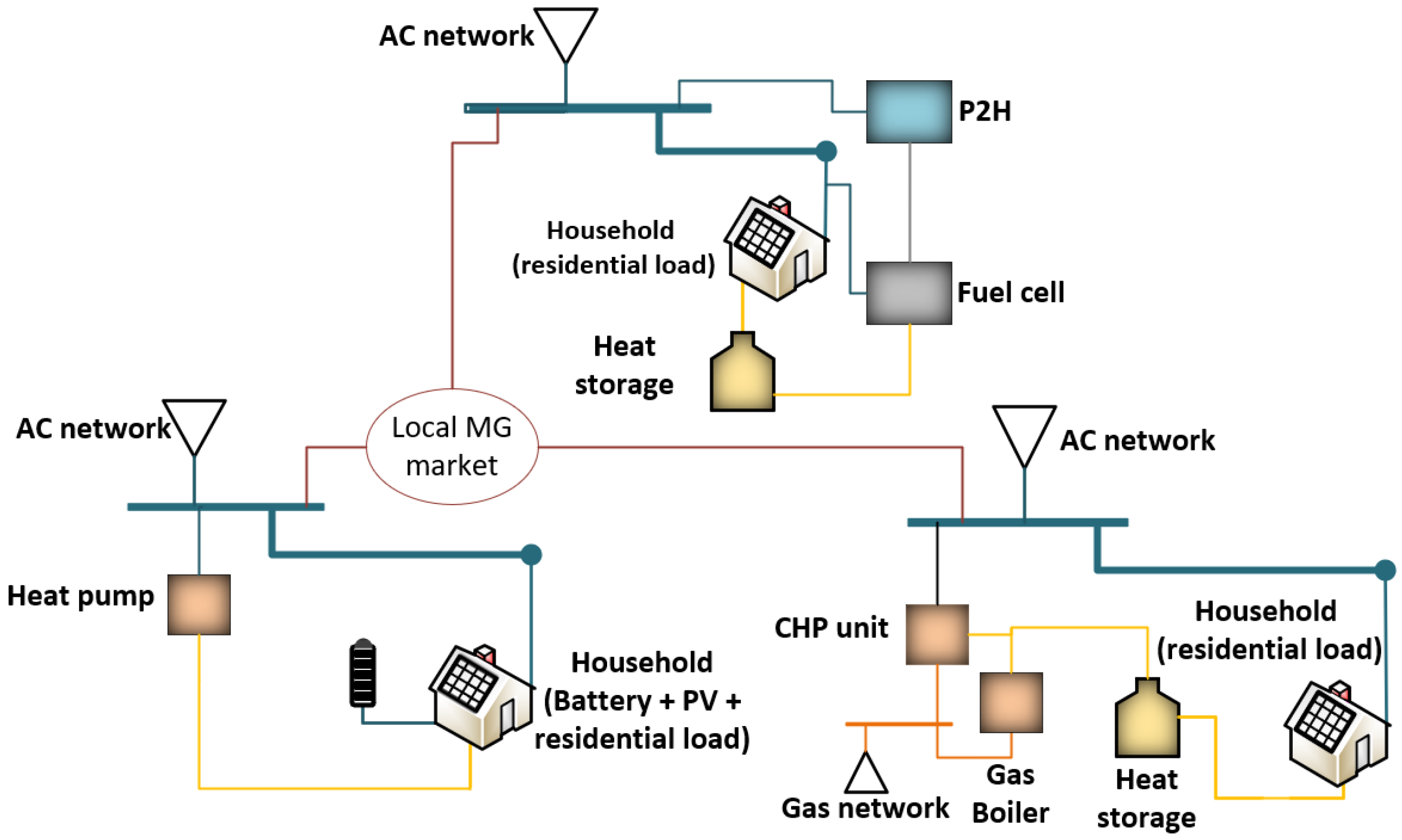
The principal concept of MES MG cooperation is that multiple MGs trade between each other on the local energy market (LEM). The MGs also participate in an upstream power exchange in terms of the day-ahead market (DAM), as shown in Figure 1. The flow of different energy vectors is defined with coloured lines on the figure: blue for electricity; orange for gas; yellow for heat; grey for hydrogen; and red for the local energy market. Energy conversion devices are represented with square boxes and storage units with tank shapes. The model developed in this paper considered the uncertainty of RES production, MG consumption and electricity price. Forecasting the errors of production and consumption patterns can lead to an imbalance of planned electricity imports and exports, which may lead to penalties. Electricity price forecasts are used for the positioning of MGs on an electricity DAM. The cooperation of different MGs could thus lead to a reduction in the risk related to forecasting uncertainty.
The model was a two-stage stochastic mixed-integer linear model. Optimisation dealt with the uncertainties by utilising stochastic scenarios in two stages. In the first stage, the decision was made before the realisation of the uncertainty and considering stochastic scenarios. The second stage optimised MG scheduling after the realisation of the stochastic scenarios while considering the decisions from the first stage. The variables in the first stage were persistent in all scenarios and the second stage variables were different for all scenarios.
3.2. Mathematical Formulation
MGs can have different devices to satisfy their various demands. The devices in each MG were defined beforehand by adding the associated variables and constraints to the model of that MG. The energy conversion devices in the model were limited with the maximum and minimum input power presented in (1). The devices included were: a heat pump (HP); a combined heat and power unit (CHP); a boiler; a power-to-hydrogen unit (PtH); and a fuel cell (FC). The charging and discharging power of the storage devices and the state of energy variables were also limited by Equation (1). They were included in battery storage systems and heat storage and hydrogen storage models. The charging and discharging of a storage device could not take place at the same time, thus Equation (2) was added for each storage device. The volume of energy contained in the storage devices (SOE) was calculated using Equation (3), where and denote the charging and discharging efficiencies, if needed. In the aforementioned constraints, “var” is the continuous variable of production/consumption for a specific device and “Xvar” represents the binary variable that indicates if the device is operating. The superscript “c” and “d” in (2) and (3) denote the charge and discharge, respectively. An extra binary variable (start) was needed for the boiler and CHP in order to model their start-up costs. Equation (4) modelled this behaviour by setting the binary variable to “1” if the device had started in that time step. The input and output relationship of the device was different for each of them. The HP used the coefficient of performance (COP) to calculate output power shown in (5). The output from the boiler and the PtH was reduced from their input based on their efficiency, as shown in (6) and (7). The CHP and FC produced two different energy outputs: electricity and heat. They were calculated with two efficiencies, one for electricity and one for heat, as shown in (8) and (9). In Equations (5) and (6), the superscript “O” denotes the output variable. Please note that in order to reduce the number of variables in the model, the output variables were virtual, i.e., they were not added to the model and were replaced with appropriate expressions.
The interconnections between the devices were handled with energy balancing equations for each energy vector that was present in a specific MG. Each MG was planned based on specific energy vectors: electricity, gas, heat and hydrogen. The devices were either found in households, such as HPs, or there was one centralised unit for the entire MG. Those that were found in households had their value multiplied by the number of households. The heat balance between production and consumption is shown in Equation (10). The electricity balance equation for each hour is presented in (11), summing all of the production and consumption of electricity and exchanging any surpluses and deficits with the electricity market, as well as trading between each MG. The hydrogen energy vector was specific because it could not be bought or sold on any market, thus all produced hydrogen had to be either be consumed or stored, which was enforced with (12). Lastly, the gas energy balance is defined with (13). The gas consumption was summed for the entire optimisation horizon because gas is bought in a single bid for a 24-h period on the day-ahead market. The gas and electricity bid variables (, and ) were decision variables in the first stage and, as such, had to be valid in each scenario. All other variables were second stage variables. The MGs mutually traded via the variables and . The volume that was sold by the MGs had to be equal to the volumes that were bought by the other MGs, which was enforced by (14).
The main goal of the optimisation was to reduce the expected operational costs by considering uncertainty scenarios. The objective function would change sightly depending on different cases, as explained in Section 4, but the general objective function is shown with (15) as the sum of electricity and gas bought/sold from/to the day-ahead market (DAM) multiplied by the price and probability in that scenario. The electricity bought from the DAM had an additional cost in terms of transmission and distribution network charges. The CHP and boiler start-up costs were also included in the objective function. Please note that in some cases (e.g., yearly analysis), the model would not be considered stochastic but deterministic. In those cases, the same mathematical formulation could be used, considering only one scenario with the probability of “1”.
4. Case Studies
The case studies consisted of three MGs following different decarbonisation strategies, as shown in Figure 1. The MGs were considered to be placed in the city of Zagreb, Croatia, and most of the input data were adapted to that city. Each MG was considered as a single low-voltage derivative with 30 households. All of the MGs had a PV unit on every household. The first MG was fully electric and, in addition to the above, contained a battery storage system and heat pump for supplying heating. Heat pump and battery storage systems are localised for each household in an MG. The second MG uses natural gas in the CHP unit for heat and electricity production and in the boiler for heat production. It also utilised heat storage. The third MG used hydrogen technologies. The electrolyser produced hydrogen using electricity, while the fuel cell transformed energy from hydrogen to heat and electricity. It also had hydrogen storage for surplus hydrogen.
The parameters of these devices are summarised in Table 1. Each household contained a PV system with a rated power of 5 kW. The heating units in the MGs were sized so they could provide 10 kW of heating per household, considering efficiencies. The boiler unit was used to support the CHP, so its input power was lower. On summer days when there was no need for heating, the CHP and fuel cell could operate with a thermal efficiency of “0”. The battery storage system was sized so that it had 1 kW and 1 kWh for every 1 kW of installed PV. The heat storage size was determined so it could store an hour’s worth of heat from the CHP. The electrolyser was sized so that it could supply enough hydrogen for the fuel cell for each hour, and the hydrogen storage was sized so that it could store 2 h worth of hydrogen from the electrolyser. The PV production, electricity load and day-ahead electricity price were considered stochastic parameters. The scenarios for PV production were created using [43] with weather data for the city of Zagreb. The electricity load profiles for the households were generated using “LoadProfileGenerator” software [44]. Lastly, the electricity price scenarios were generated with the SARIMA model, using electricity prices from the Croatian power exchange (CROPEX) [45]. A set of prices from 2021 was used, concluding with prices from 12 November. The year 2021 was chosen so as to better follow current price trends, since the average electricity price increased from EUR 50 MWh in 2019 to EUR 100 MWh and, in the last few months of 2021, to EUR 200 MWh. Each stochastic parameter was made into three scenarios, where the electricity load and PV production had different scenarios for each MG. The electricity price, load and PV production scenarios were combined into nine scenarios with equal probability. The gas price was taken from CEGH VTP (Central European Gas Hub Virtual Trading Point) [46] as an average daily price from 30 September to 13 November, and amounted to EUR 85 MWh. The heat consumption was taken from [47] for the city of Indianapolis, USA, since it has a similar climate to Zagreb, Croatia. The transmission and distribution network prices were those set by Croatian TSO and DSO, and were equal to EUR 12 MWh and EUR 29 MWh, respectively. The specific CO2 emission for the electricity bought from the electricity market was 0.177 kg/kWh [48] and for natural gas was 0.202 kg/kWh [49].
The case study considered two different analyses: a daily stochastic analysis and a yearly analysis. The daily analysis had six different cases, each considering one summer day and one winter day. The yearly analysis had four cases.
The daily stochastic analyses were as follows:
- Case 0 (C0) was a benchmark case with no flexibility nor electricity and hydrogen production. All MGs could only buy electricity from the DAM, they did not have any type of storage and they only used boilers to satisfy heat demand. We did not consider any uncertainty and all scenarios were averaged into one deterministic scenario.
- Case 1 (C1) considered MGs with the architectures described in this chapter. As with C0, it did not consider any uncertainty nor could it trade between MGs. It relied on a technique similar to the concept of net metering for electricity billing, in which a surplus of electricity returned to the grid could be used later to lower the consumer’s bill. In our model, net metering was modelled as a virtual storage system in which MGs could withdraw their past surpluses whenever necessary, i.e., netted electricity from a summer day could be transferred to a winter day.
- Case 2 (C2) was a stochastic case utilising scenarios. It could freely trade on the electricity market and between MGs.
- Case 3 (C3) was a sensitivity analysis focused on the gas price increase compared to C2. Two instances were considered. In the first, the price of gas was equal to the average price of electricity (C3.1) while in the second, a price 50% higher than the average price of electricity was considered in the described scenarios (C3.2). The prices amounted to EUR 199 MWh and EUR 298 MWh, respectively.
- Case 4 (C4) was similar to C2; however, it considered that the MGs were located further apart so they had to pay distribution network charges when buying electricity from each other.
- Case 5 (C5) expanded on C4 and considered that the MGs were dislocated and had to pay transmission and distribution network charges when/if buying electricity from each other.
The yearly analyses were as follows:
- Yearly case 1 (Y1) was a yearly analysis based on C2, but without considering any uncertainty.
- Yearly case 2 (Y2) was similar to Y1, with the main difference being that the objective function was changed to maximising self-sufficiency. This meant that the objective function in the model was to minimise the volumes of electricity and gas bought from the DAMs without considering prices. The total costs were calculated after the optimisation.
- Yearly case 3 (Y3) was again similar to Y1, but this time the main difference was that the objective function was the minimisation of CO2 emissions. The total costs were calculated after the optimisation.
- Yearly case 4 (Y4) was the same as Y1, but instead of three different MGs, it optimised three MGs of the same kind. This case had three instances: the first with three electric MGs (Y4.E); the second with three gas MGs (Y4.G); and lastly, an instance with three hydrogen MGs (Y4.H).
5. Discussion and Results
This section discusses the results of the case studies. The first three subsections present the results from the daily analyses, focusing on the total operating cost, trading on the DAM and local market and multi-energy flexibility and emissions while dealing with uncertainties. The fourth subsection details the yearly analyses and presents how the different approaches affected the total operating cost, emissions and self-sufficiency. The model was written in Python 3.8 and used the Gurobi 9 optimisation solver [50]. The PC specifications were: AMD Ryzen 5 3600 6-Core 3.59 GHz processor with 16 GB of RAM. The computational time of the stochastic models was around 10 s, while the yearly analyses had a computational time of around 2 min.
5.1. Daily Analyses for the First Three Cases
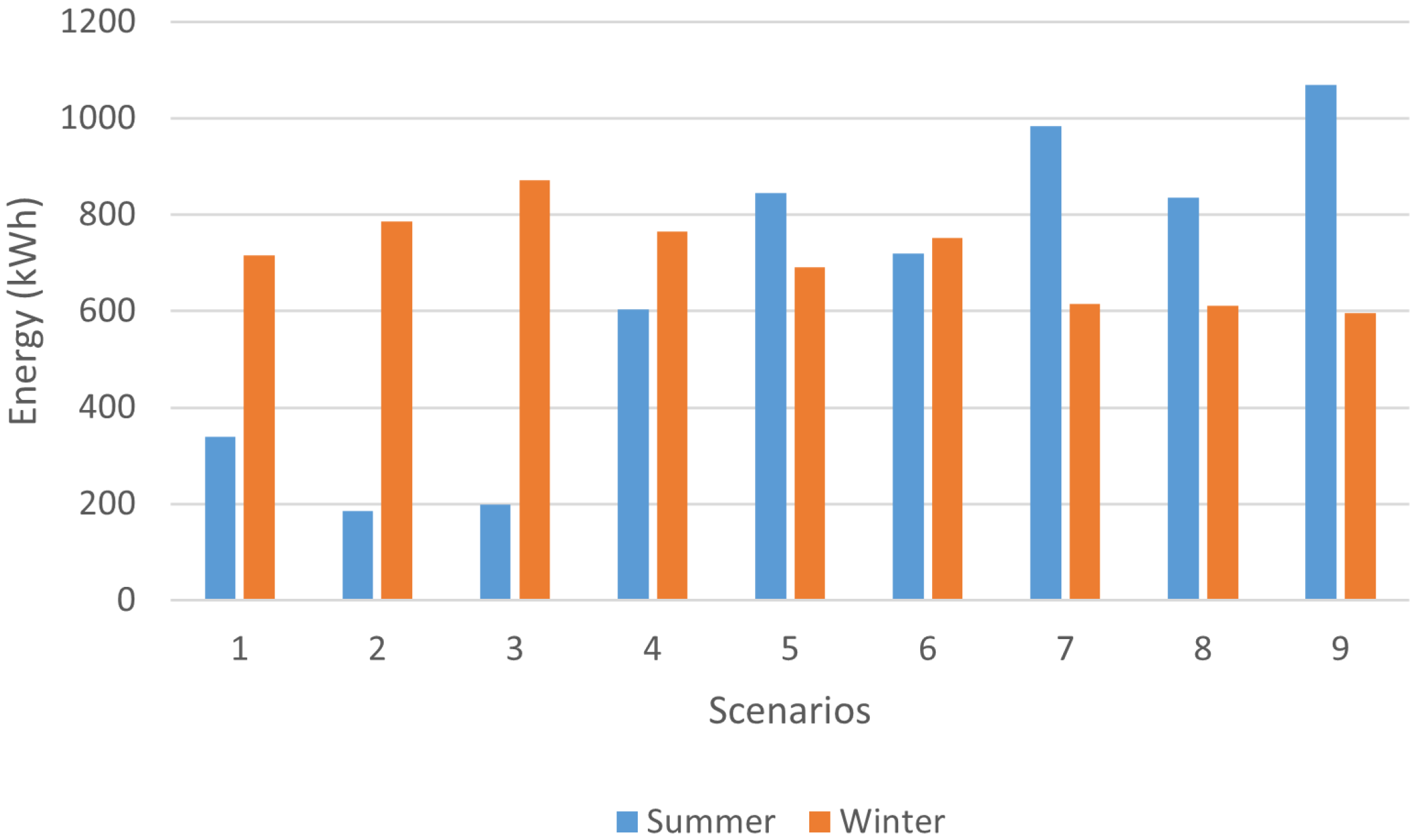
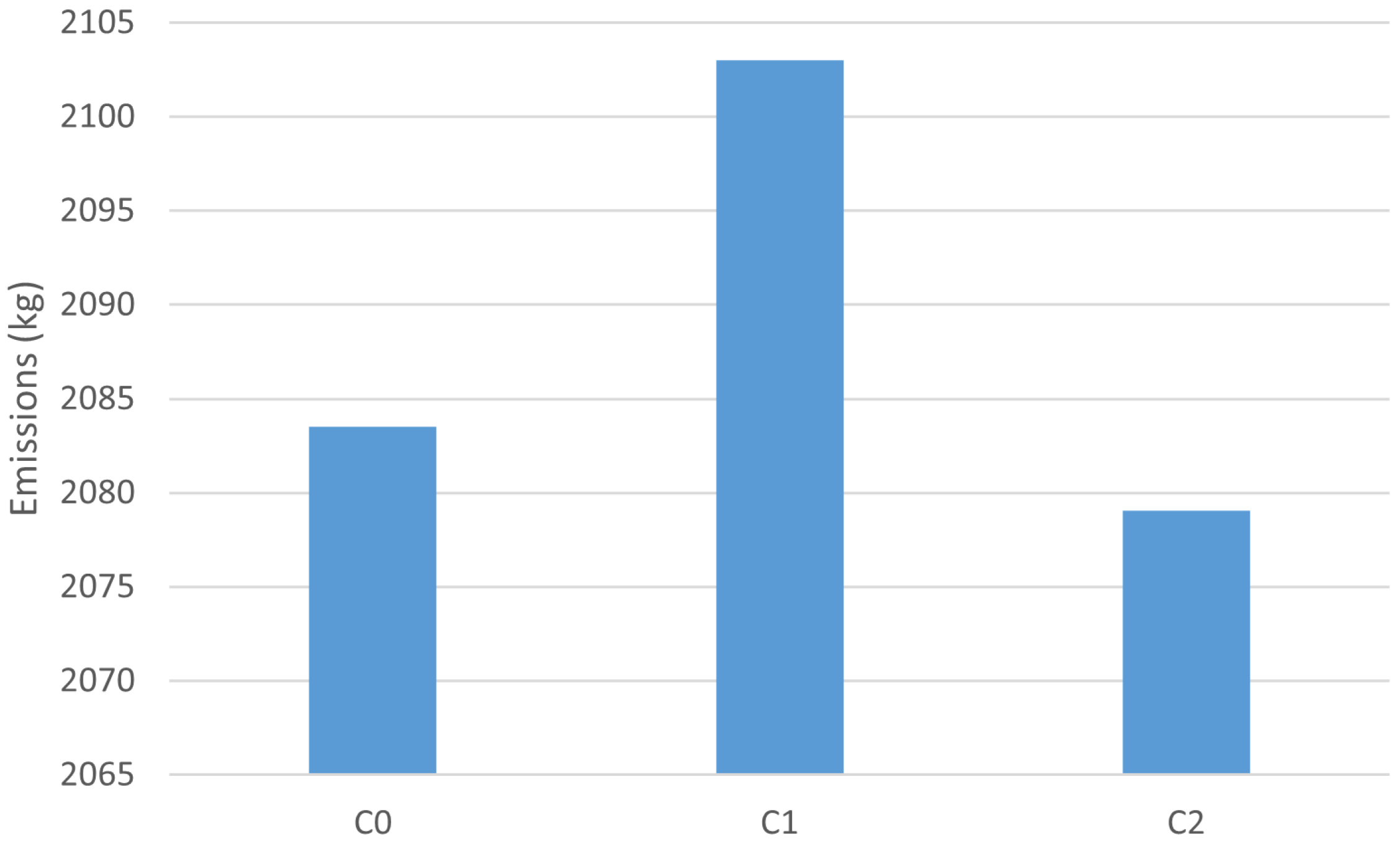
The first analysis compared C2 to C0 and C1. Table 2 shows the costs per MG for each case on a summer and on a winter day. On a summer day, C2 proved to be much better than the other two cases, while on a winter day, it performed worse than C0 and C1. By adding the cost of both days, we observed that C2 performed 20% worse than C0 and 13% better than C1. The fact that C0 managed to outperform C2 could be explained by the difference between deterministic and stochastic optimisation. As previously mentioned, C2 was a stochastic case study, unlike C0 and C1, which were deterministic. Stochastic models are intrinsically worse than deterministic models since they must adhere to a wide variety of scenarios and be feasible for each of them. In our model, this meant that the stochastic model had to take advantage of all flexibilities that it has at its disposal, which led to higher costs. Please note that neither C0 nor C1 would be able to adhere for all scenarios at once if subjected to stochastic analysis, or would perform very poorly. Although hindered by uncertainties, C2 performed much better than C1 because it could fully utilise all of its production and flexibility on the DAM, while C1 was left with unused netted energy at the end of the optimisation horizon. Figure 2 shows the total energy traded between the MGs in the case of C2, which was the best way to demonstrate the flexibility and the adjustments made to the uncertainties. The gas MG had the lowest local import volumes, on average, for both summer and winter days, while the hydrogen MG had the highest local import in summer and the electric MG had the highest in winter. The gas and hydrogen MGs mostly exported electricity to other MGs on winter days because of their controllable generation from the CHP and fuel cell. On summer days, the electric and gas MGs were the forerunners in exports so as to offset the hydrogen MG’s lack of flexibility. From this, it can be concluded that the CHP outperforms the fuel cell in the summer and provides more flexibility in the winter. This is mostly influenced by the price of gas being lower than the price of electricity, on average, and by its invariability. For this reason, we conducted a gas price sensitivity analysis in C3 and discuss it in the following subsection. The import and export ratio is summarised in Table 3. The total emissions are shown in Figure 3. C2’s emissions were fairly similar to C0, being only 0.2% lower, and 1.1% lower than C1. The reductions in emissions, though small, was a consequence of the optimisation trying to lower its costs.
5.2. Daily Analysis for Case 3
For the two subcases of Case 3, the gas price was set to be equal to the average price of electricity, reflecting the realistic situation of the markets over the last couple of months of 2021. The total costs of both C3 cases increased as expected due to higher gas prices, as shown in Table 4. An interesting point to note here is that in the summer, the total energy import was much lower than in C2 while in the winter, it was almost the same. This was because the CHP was not being used in the summer due to the price increase, while in the winter, gas consumption was a little lower but was still needed since the gas MG did not have any alternative options for thermal production. This was also reflected in the total cost, where the winter had a much higher cost difference. In the summer, local import increased in favour of selling to the DAM in order to replace the flexibility missing from the lower CHP usage. In the winter, local trade was lower because the marginal price of the most prominent flexibility provider (CHP) increased, thus lowering the potential for local trade. The effect of the gas price increase was that it lowered emissions by 6% in C3.1 and 6.2% in C3.2. This was mostly attributed to the lower gas consumption in summer.
5.3. Daily Analysis for Cases Four and Five
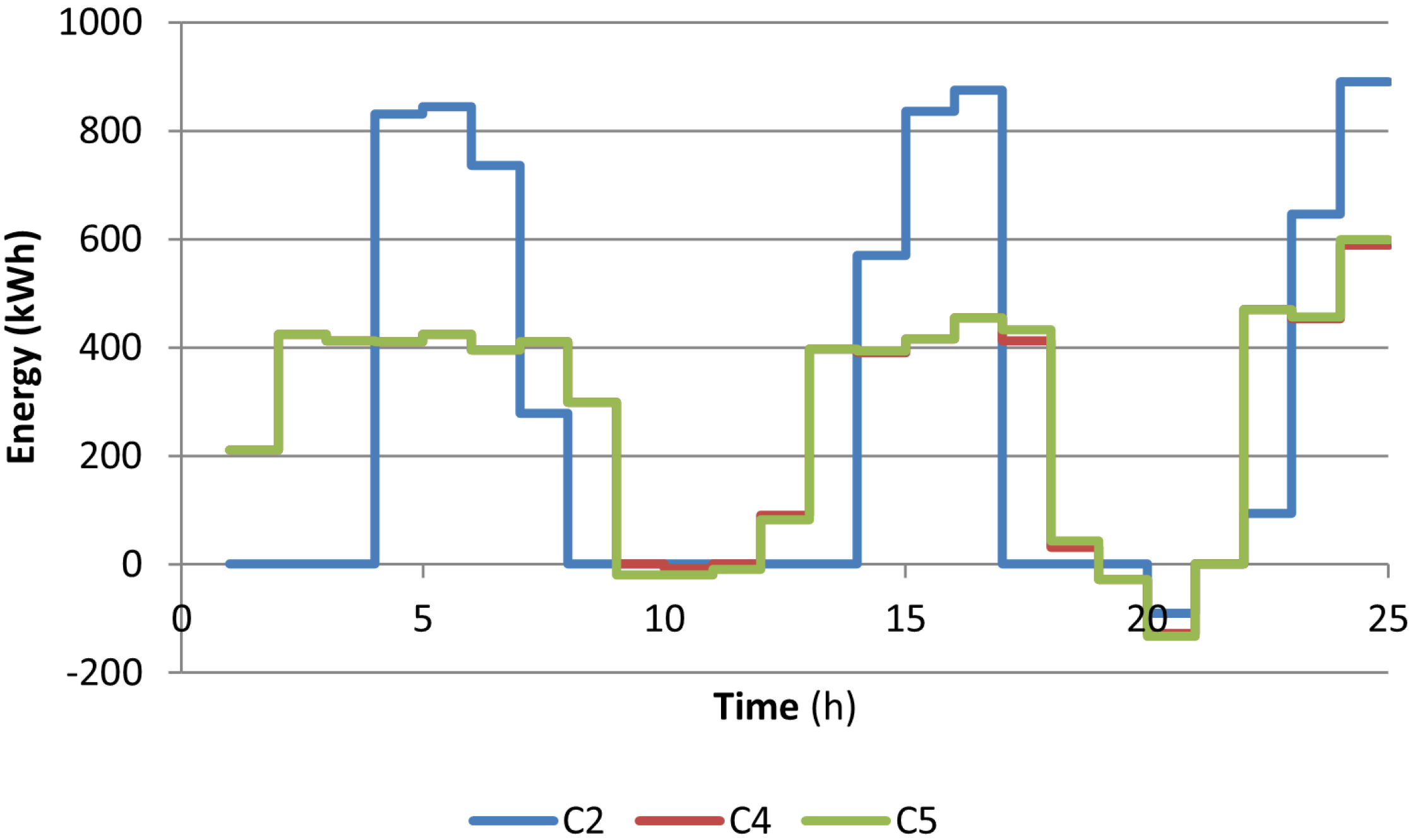
Adding new constraints in cases C4 and C5 raised the total costs, as shown in Table 5. Although the increase in cost was not significant, other parameters have changed. Since local trading became more expensive, the gas MG was selling more volume to the DAM than to the local market. Concurrently, the electric and hydrogen MGs were replacing the deficit from the local market with purchases from the DAM. Additionally, the MGs were more reliant on their own flexibility than on the shared flexibility from the different energy vectors. Similarly, the MGs had to disperse their DAM schedule instead of trading at more favourable times. This is seen in Figure 4 and Figure 5, where the C2 curve is more steep than those of C4 and C5. The conclusion to be made here is that, although the schedule of MGs changed significantly, the overall costs did not rise, meaning that the system was showing a significant level of robustness. With the increase in DAM imports and decrease in local imports, the emissions in C4 rose by 3% compared to C2 and by 3.77% compared to C5.
5.4. Yearly Analysis
The yearly analysis Y1 followed a similar trend as that seen in the daily analyses. The gas MG was the biggest exporter on the local market, while the others were mostly importing from it. Flexibility was used to lower imports to the DAM by adjusting the optimal trade in times. When constrained to a different optimisation approach, i.e., increasing self-sufficiency and lowering emissions, it changed its behaviour, which is shown in Table 6. Both alternative approaches, Y2 and Y3, yielded similar results. Both managed to lower DAM imports and emissions to a similar level, although only one of those goals was set in the objective function. The cost increase was also fairly equal between those two cases. Interestingly, the gas volumes changed a lot between all three cases. The key aspect that differentiated Y2 and Y3 was that Y2 favoured DAM exports over local trading, while Y3 was the opposite. Nevertheless, both cases showed a significant drop in DAM exports. The results from the Y2 and Y3 analyses show that these goals were somewhat correlated to one another.
In the Y4 analysis, it was shown that the purely electric MG (Y4.E) performed the best in terms of total cost and emissions. The gas MG (Y4.G) had a lower total cost than Y1, but at the cost of higher emissions. Lastly, the hydrogen MG (Y4.H) had the highest cost and emissions compared to all of the other cases. The results from the Y4 analysis are summarised in Table 7.
6. Conclusions
The paper aimed to present different decarbonisation techniques for microgrids. We selected three extreme cases: one based on a purely electric architecture, one on a gas architecture and lastly, one on a hydrogen architecture. The local electricity market was included as a way of coupling these MGs together, with the idea that the MGs could provide flexibility between each other without additional costs. Daily and yearly analyses are presented, which analyse different realistic market and system situations. The results are presented in three relevant key performance indicators: the total cost of operation, self-sufficiency and CO2 emissions. On a yearly level, the conclusions were made that DAM-oriented trading outperformed the electricity netting approach by approximately 13%. This conclusion was confirmed in the sensitivity analyses, where the gas price increased to the record levels noted during the second half of 2021. While the total costs of MG operation increased, the emissions decreased. In the second set of analyses, we ran annual analyses and considered three different optimisation goals showcasing the different mindsets of potential MG investors. When the MG operation was driven either by self-sufficiency or emission reduction goals, the results were very similar. However, they were majorly different from the objective of cost minimisation. Lastly, all decarbonisation MG options were compared to each other by running daily optimisations. The results clearly show that the electric MG performed the best, while the hydrogen MG was the worst. The gas MG option was indicated as a good way to balance RES during the transition towards a highly renewable energy system; however, they were characterised by high dependency on gas prices and much higher emissions.
Author Contributions
Conceptualization and methodology, all authors; software, M.K. and L.H.; validation, all authors; formal analysis, M.K.; investigation and resources, M.K. and L.H.; data curation, M.K. and L.H.; writing—original draft preparation, M.K. and L.H.; writing—review and editing, all authors; visualization, M.K.; supervision, project administration and funding acquisition, T.C. All authors have read and agreed to the published version of the manuscript.
Funding
This research received no external funding.
Institutional Review Board Statement
Not applicable.
Informed Consent Statement
Not applicable.
Data Availability Statement
Not applicable.
Acknowledgments
This work was funded by the European Union through the European Regional Development Fund for the Competitiveness and Cohesion Operational Programme 2014–2020 of the Republic of Croatia under project No. KK.01.1.1.07: “Universal Communication and Control System for Industrial Facilities”. The content of this work is the sole responsibility of the University of Zagreb, Faculty of Electrical Engineering and Computing.
Conflicts of Interest
The authors declare no conflict of interest.
Abbreviations
The following abbreviations are used in this manuscript:
| Indices and Variables | |
| Set and index for scenarios | |
| Set and index for microgrids | |
| Set and index for hours | |
| Input power of boiler in scenario , MG m and time t | |
| Input power of PtH in scenario , MG m and time t | |
| Input power of CHP in scenario , MG m and time t | |
| Input power of FC in scenario , MG m and time t | |
| Input power of HP in scenario , MG m and time t | |
| Heat storage input power in scenario , MG m and time t | |
| Heat storage output power in scenario , MG m and time t | |
| Battery storage input power in scenario , MG m and time t | |
| Battery storage output power in scenario , MG m and time t | |
| Hydrogen storage input power in scenario , MG m and time t | |
| Hydrogen storage output power in scenario , MG m and time t | |
| Gas volume bought from day-ahead market in MG m | |
| Electricity volume bought from day-ahead market in MG m and time t | |
| Electricity volume sold to day-ahead market in MG m and time t | |
| Electricity volume bought from local MG market in scenario , MG m and time t | |
| Electricity volume sold to local MG market in scenario , MG m and time t | |
| Parameters | |
| Boiler efficiency coefficient | |
| PtH efficiency coefficient | |
| CHP electricity output efficiency coefficient | |
| CHP heat output efficiency coefficient | |
| FC electricity output efficiency coefficient | |
| FC heat output efficiency coefficient | |
| HP coefficient of performance | |
| Number of household in MG m | |
| Household load in scenario , MG m and time t | |
| PV production in scenario , MG m and time t | |
| Heat demand in MG m and time t | |
| Electricity price in scenario , MG m and time t | |
| G | Price of gas |
| Probability of scenario | |
| Transmission network charges | |
| Distribution network charges |
References
- Pavić, I.; Beus, M.; Pandžić, H.; Capuder, T.; Štritof, I. Electricity markets overview—Market participation possibilities for renewable and distributed energy resources. In Proceedings of the 2017 14th International Conference on the European Energy Market (EEM), Dresden, Germany, 6–9 June 2017; pp. 1–5. [Google Scholar] [CrossRef]
- Mancarella, P.; Chicco, G. Real-Time Demand Response from Energy Shifting in Distributed Multi-Generation. IEEE Trans. Smart Grid 2013, 4, 1928–1938. [Google Scholar] [CrossRef]
- Herenčić, L.; Melnjak, M.; Capuder, T.; Andročec, I.; Rajšl, I. Techno-economic and environmental assessment of energy vectors in decarbonization of energy islands. Energy Convers. Manag. 2021, 236, 114064. [Google Scholar] [CrossRef]
- Good, N.; Karangelos, E.; Navarro-Espinosa, A.; Mancarella, P. Optimization under Uncertainty of Thermal Storage-Based Flexible Demand Response with Quantification of Residential Users’ Discomfort. IEEE Trans. Smart Grid 2015, 6, 2333–2342. [Google Scholar] [CrossRef]
- Holjevac, N.; Capuder, T.; Zhang, N.; Kuzle, I.; Kang, C. Corrective receding horizon scheduling of flexible distributed multi-energy microgrids. Appl. Energy 2017, 207, 176–194. [Google Scholar] [CrossRef]
- Capuder, T.; Mancarella, P. Assessing the benefits of coordinated operation of aggregated distributed Multi-energy Generation. In Proceedings of the 2016 Power Systems Computation Conference (PSCC), Genoa, Italy, 20–24 June 2016; pp. 1–7. [Google Scholar] [CrossRef]
- Hirsch, A.; Parag, Y.; Guerrero, J. Microgrids: A review of technologies, key drivers, and outstanding issues. Renew. Sustain. Energy Rev. 2018, 90, 402–411. [Google Scholar] [CrossRef]
- Sachs, J.; Sawodny, O. Multi-objective three stage design optimization for island microgrids. Appl. Energy 2016, 165, 789–800. [Google Scholar] [CrossRef]
- Parisio, A.; Del Vecchio, C.; Vaccaro, A. A robust optimization approach to energy hub management. Int. J. Electr. Power Energy Syst. 2012, 42, 98–104. [Google Scholar] [CrossRef]
- Mancarella, P. MES (multi-energy systems): An overview of concepts and evaluation models. Energy 2014, 65, 1–17. [Google Scholar] [CrossRef]
- Mancarella, T.C.P. Techno-economic and environmental modelling and optimization of flexible distributed multi-generation options. Energy 2014, 71, 516–533. [Google Scholar] [CrossRef]
- Mancarella, P.; Chicco, G.; Capuder, T. Arbitrage opportunities for distributed multi-energy systems in providing power system ancillary services. Energy 2018, 161, 381–395. [Google Scholar] [CrossRef]
- Holjevac, N.; Capuder, T.; Kuzle, I. Defining Key Parameters of Economic and Environmentally Efficient Residential Microgrid Operation. Energy Procedia 2017, 105, 999–1008. [Google Scholar] [CrossRef]
- Shilaja, C.; Arunprasath, T.; Priya, P. Day-ahead optimal scheduling of microgrid with adaptive grasshopper optimization algorithm. Int. J. Commun. Syst. 2019, 35, e4133. [Google Scholar]
- Karimi, A.; Khayat, Y.; Naderi, M.; Dragičević, T.; Mirzaei, R.; Blaabjerg, F.; Bevrani, H. Inertia Response Improvement in AC Microgrids: A Fuzzy-Based Virtual Synchronous Generator Control. IEEE Trans. Power Electron. 2020, 35, 4321–4331. [Google Scholar] [CrossRef]
- Daneshvar, M.; Mohammadi-Ivatloo, B.; Asadi, S.; Anvari-Moghaddam, A.; Rasouli, M.; Abapour, M.; Gharehpetian, G.B. Chance-constrained models for transactive energy management of interconnected microgrid clusters. J. Clean. Prod. 2020, 271, 122177. [Google Scholar] [CrossRef]
- Karimi, H.; Jadid, S. Optimal energy management for multi-microgrid considering demand response programs: A stochastic multi-objective framework. Energy 2020, 195, 116992. [Google Scholar] [CrossRef]
- Daneshvar, M.; Mohammadi-ivatloo, B.; Zare, K.; Asadi, S.; Anvari-Moghaddam, A. A Novel Operational Model for Interconnected Microgrids Participation in Transactive Energy Market: A Hybrid IGDT/Stochastic Approach. IEEE Trans. Ind. Inform. 2020, 17, 4025–4035. [Google Scholar] [CrossRef]
- Khorasany, M.; Najafi-Ghalelou, A.; Razzaghi, R.; Mohammadi-Ivatloo, B. Transactive Energy Framework for Optimal Energy Management of Multi-Carrier Energy Hubs under Local Electrical, Thermal, and Cooling Market Constraints. Int. J. Electr. Power Energy Syst. 2021, 129, 106803. [Google Scholar] [CrossRef]
- Zare Oskouei, M.; Mirzaei, M.A.; Mohammadi-Ivatloo, B.; Shafiee, M.; Marzband, M.; Anvari-Moghaddam, A. A hybrid robust-stochastic approach to evaluate the profit of a multi-energy retailer in tri-layer energy markets. Energy 2021, 214, 118948. [Google Scholar] [CrossRef]
- Zhu, D.; Yang, B.; Liu, Q.; Ma, K.; Zhu, S.; Ma, C. Energy trading in microgrids for synergies among electricity, hydrogen and heat networks. Appl. Energy 2020, 272, 115225. [Google Scholar] [CrossRef]
- Karimi, H.; Bahmani, R.; Jadid, S.; Makui, A. Dynamic transactive energy in multi-microgrid systems considering independence performance index: A multi-objective optimization framework. Int. J. Electr. Power Energy Syst. 2020, 126, 106563. [Google Scholar] [CrossRef]
- Yang, Z.; Hu, J.; Ai, X.; Wu, J.; Yang, G. Transactive Energy Supported Economic Operation for Multi-Energy Complementary Microgrids. IEEE Trans. Smart Grid 2021, 12, 4–17. [Google Scholar] [CrossRef]
- Cheng, Y.; Zhang, P.; Liu, X. Collaborative Autonomous Optimization of Interconnected Multi-Energy Systems with Two-Stage Transactive Control Framework. Energies 2020, 13, 171. [Google Scholar] [CrossRef] [Green Version]
- Guo, J.; Tan, J.; Lia, Y.; Gu, H.; Liu, X.; Cao, Y.; Yan, Q.; Xu, D. Decentralized Incentive-based multi-energy trading mechanism for CCHP-based MG cluster. Int. J. Electr. Power Energy Syst. 2021, 133, 107138. [Google Scholar] [CrossRef]
- Naz, K.; Zainab, F.; Mehmood, K.K.; Bukhari, S.B.A.; Khalid, H.A.; Kim, C.H. An Optimized Framework for Energy Management of Multi-Microgrid Systems. Energies 2021, 14, 6012. [Google Scholar] [CrossRef]
- Smith, E.; Robinson, D.; Agalgaonkar, A. Cooperative Control of Microgrids: A Review of Theoretical Frameworks, Applications and Recent Developments. Energies 2021, 14, 8026. [Google Scholar] [CrossRef]
- Khorasany, M.; Mishra, Y.; Ledwich, G. Market Framework for Local Energy Trading: A Review of Potential Designs and Market Clearing Approaches. IET Gener. Transm. Distrib. 2018, 12, 5899–5908. [Google Scholar] [CrossRef] [Green Version]
- Zhang, C.; Wu, J.; Zhou, Y.; Cheng, M.; Long, C. Peer-to-Peer energy trading in a Microgrid. Appl. Energy 2018, 220, 1–12. [Google Scholar] [CrossRef]
- Dudjak, V.; Neves, D.; Alskaif, T.; Khadem, S.; Pena-Bello, A.; Saggese, P.; Bowler, B.; Andoni, M.; Bertolini, M.; Zhou, Y.; et al. Impact of local energy markets integration in power systems layer: A comprehensive review. Appl. Energy 2021, 301, 117434. [Google Scholar] [CrossRef]
- Hayes, B.; Thakur, S.; Breslin, J. Co-simulation of electricity distribution networks and peer to peer energy trading platforms. Int. J. Electr. Power Energy Syst. 2020, 115, 105419. [Google Scholar] [CrossRef]
- Pilehvar, M.S.; Mirafzal, B. PV-Fed Smart Inverters for Mitigation of Voltage and Frequency Fluctuations in Islanded Microgrids. In Proceedings of the 2020 International Conference on Smart Grids and Energy Systems (SGES), Perth, Australia, 23–26 November 2020; pp. 807–812. [Google Scholar] [CrossRef]
- Bani-Ahmed, A.; Weber, L.; Nasiri, A.; Hosseini, H. Microgrid communications: State of the art and future trends. In Proceedings of the 2014 International Conference on Renewable Energy Research and Application (ICRERA), Milwaukee, WI, USA, 19–22 October 2014; pp. 780–785. [Google Scholar] [CrossRef]
- Safdar, S.; Hamdaoui, B.; Cotilla-Sanchez, E.; Guizani, M. A survey on communication infrastructure for micro-grids. In Proceedings of the 2013 9th International Wireless Communications and Mobile Computing Conference (IWCMC), Sardinia, Italy, 1–5 July 2013; pp. 545–550. [Google Scholar] [CrossRef]
- Marzal, S.; Salas, R.; González-Medina, R.; Garcerá, G.; Figueres, E. Current challenges and future trends in the field of communication architectures for microgrids. Renew. Sustain. Energy Rev. 2018, 82, 3610–3622. [Google Scholar] [CrossRef] [Green Version]
- Garau, M.; Celli, G.; Ghiani, E.; Pilo, F.; Corti, S. Evaluation of Smart Grid Communication Technologies with a Co-Simulation Platform. IEEE Wirel. Commun. 2017, 24, 42–49. [Google Scholar] [CrossRef]
- Li, W.; Ferdowsi, M.; Stevic, M.; Monti, A.; Ponci, F. Cosimulation for Smart Grid Communications. IEEE Trans. Ind. Inform. 2014, 10, 2374–2384. [Google Scholar] [CrossRef]
- Bhattarai, B.P.; Lévesque, M.; Bak-Jensen, B.; Pillai, J.R.; Maier, M.; Tipper, D.; Myers, K.S. Design and Cosimulation of Hierarchical Architecture for Demand Response Control and Coordination. IEEE Trans. Ind. Inform. 2017, 13, 1806–1816. [Google Scholar] [CrossRef]
- Findrik, M.; Smith, P.; Kazmi, J.H.; Faschang, M.; Kupzog, F. Towards secure and resilient networked power distribution grids: Process and tool adoption. In Proceedings of the 2016 IEEE International Conference on Smart Grid Communications (SmartGridComm), Sydney, Australia, 6–9 November 2016; pp. 435–440. [Google Scholar] [CrossRef]
- Kuzlu, M.; Pipattanasomporn, M. Assessment of communication technologies and network requirements for different smart grid applications. In Proceedings of the 2013 IEEE PES Innovative Smart Grid Technologies Conference (ISGT), Washington, DC, USA, 24–27 February 2013; pp. 1–6. [Google Scholar] [CrossRef]
- Jogunola, O.; Ikpehai, A.; Anoh, K.; Adebisi, B.; Hammoudeh, M.; Son, S.Y.; Harris, G. State-Of-The-Art and Prospects for Peer-To-Peer Transaction-Based Energy System. Energies 2017, 10, 2106. [Google Scholar] [CrossRef] [Green Version]
- Ho, Q.D.; Gao, Y.; Le-Ngoc, T. Challenges and research opportunities in wireless communication networks for smart grid. IEEE Wirel. Commun. 2013, 20, 89–95. [Google Scholar] [CrossRef]
- Pfenninger, S.; Staffell, I. Long-term patterns of European PV output using 30 years of validated hourly reanalysis and satellite data. Energy 2016, 114, 1251–1265. [Google Scholar] [CrossRef] [Green Version]
- Pflugradt, N.; Muntwyler, U. Synthesizing residential load profiles using behavior simulation. Energy Procedia 2017, 122, 655–660. [Google Scholar] [CrossRef]
- Croatian Power Exchange. Available online: https://www.cropex.hr (accessed on 20 November 2021).
- Spot Market Data|CEGH VTP. Available online: https://www.powernext.com/spot-market-data (accessed on 20 November 2021).
- Office of Energy Efficiency & Renewable Energy. Commercial and Residential Hourly Load Profiles for all TMY3 Locations in the United States. Available online: tinyurl.com/ybhrjuj6 (accessed on 20 November 2021).
- Greenhouse Gas Emission Intensity of Electricity Generation by Country; European Environment Agency: København, Denmark, 2021.
- Penman, J.; Gytarsky, M.; Hiraishi, T.; Irving, W.; Krug, T. 2006 IPCC Guidelines for National Greenhouse Gas Inventories; Prepared by the National Greenhouse Gas Inventories Programme; IGES: Miuragun, Japan, 2006. [Google Scholar]
- Gurobi Optimization, LLC. Gurobi Optimizer Reference Manual; Gurobi Optimization, LLC: Beaverton, OR, USA, 2021. [Google Scholar]
Figure 1.
The layout of the MGs.

Figure 2.
The trades between MGs in C2.

Figure 3.
The total emissions of CO2 in C0, C1 and C2.

Figure 4.
The DAM schedule for summer in C2, C4 and C5.

Figure 5.
The DAM schedule for winter in C2, C4 and C5.


Table 1.
The parameters of all devices considered by the MGs.
| Device | Input Power | Efficiency | Capacity |
|---|---|---|---|
| Heat Pump (1 per household) | 4 kW | COP: 2.5 | - |
| CHP | 430 kW | Electric: 22% Thermal: 70% | - |
| Boiler | 180 kW | 85% | - |
| Fuel Cell | 580 kW | Electric: 37% Thermal: 52% | - |
| Electrolyser | 880 kW | 66% | - |
| Battery (1 per household) | Charge: 5 kW Discharge: 5 kW | Charge: 90% Discharge: 90% | 5 kWh |
| Heat Storage | Input: 335 kW Output: 335 kW | Input: 90% Output: 90% | 335 kWh |
| Hydrogen Storage | Input: 1200 kW Output: 1200 kW | No losses | 1200 kWh |
Table 2.
The total costs (EUR) for cases C0, C1 and C2.
| Summer | Winter | |||||
|---|---|---|---|---|---|---|
| MG | C0 | C1 | C2 | C0 | C1 | C2 |
| EE | 52.1 | 7.16 | −130.14 | 313.08 | 27.67 | 125.79 |
| Gas | 55.2 | 259.5 | −138.9 | 316.06 | 259.5 | 307.82 |
| H2 | 55.5 | 170.41 | −139.6 | 316.87 | 819.81 | 1310.29 |
| All 3 MGs | 162.77 | 437.07 | −408.63 | 946 | 1106.98 | 1743.9 |
Table 3.
The ratio of local import and export for each MG in C2.
| Summer | Winter | |||
|---|---|---|---|---|
| MG | Import | Export | Import | Export |
| 1 | 24.8% | 57.39% | 89.49% | 0% |
| 2 | 7.64% | 38.85% | 0.84% | 62.68% |
| 3 | 67.56% | 3.76% | 9.66% | 37.32% |
Table 4.
The C3 results and a comparison to the C2 results.
| Summer | Winter | |||
|---|---|---|---|---|
| C3.1 | C3.2 | C3.1 | C3.2 | |
| Total cost (EUR) | −387.17 | −381.26 | 2210.2 | 2565.92 |
| Difference in total cost compared to C2 | 5.54% | 7.17% | 21.09% | 32.03% |
| Total energy import difference compared to C2 | −167.28% | −167.21% | −0.45% | −0.46% |
| Total local import difference compared to C2 | 8.82% | 9.01% | −20.41% | −30.51% |
Table 5.
The C4 and C5 results and a comparison to the C2 results.
| Summer | Winter | |||
|---|---|---|---|---|
| MG | C4 | C5 | C4 | C5 |
| Total cost (EUR) | −395.56 | −390.29 | 1807.92 | 1811.88 |
| Difference in total cost compared to C2 | 3.3% | 4.7% | 3.54% | 3.75% |
| Total energy import difference compared to C2 | 19.9% | 20.02% | 0.97% | 1.91% |
| Total local import difference compared to C2 | −30.72% | −37.47% | −50.32% | −60.82% |
Table 6.
The results for yearly analyses Y1, Y2 and Y3.
| Case | Total Cost | Emissions | Local Trading | Imported from DAM | Exported to DAM | Gas Import from DAM |
|---|---|---|---|---|---|---|
| Y1 | 123,122.5 | 292,846.4 | 280,105.4 | 941,901.1 | 391,514.8 | 624,405.4 |
| Y2 | 169,751.4 | 271,612.7 | 335,118.9 | 832,733.1 | 199,390 | 614,945.4 |
| Difference between cases Y1 and Y2 | 27.47% | −7.82% | 16.42% | −13.11% | −96.36% | −1.54% |
| Y3 | 172,203.3 | 271,683.5 | 358,088.6 | 833,149.6 | 175,774 | 614,930.7 |
| Difference between cases Y1 and Y3 | 28.5% | −7.79% | 21.78% | −13.05% | −122.74% | −1.54% |
Table 7.
The results for the yearly analysis Y4 and a comparison to the Y1 results.
| Y4.E | Y4.G | Y4.H | |
|---|---|---|---|
| Total Cost (EUR) | 23,610.77 | 73,631.96 | 291,046 |
| Difference compared to Y1 | 80.82% | 40.2% | −136.39% |
| Emissions (kg) | 93,823.06 | 364,346.3 | 495,686.5 |
| Difference compared to Y1 | 67.96% | −24.42% | −69.27% |
Publisher’s Note: MDPI stays neutral with regard to jurisdictional claims in published maps and institutional affiliations. |
© 2022 by the authors. Licensee MDPI, Basel, Switzerland. This article is an open access article distributed under the terms and conditions of the Creative Commons Attribution (CC BY) license (https://creativecommons.org/licenses/by/4.0/).
Share and Cite
MDPI and ACS Style
Kostelac, M.; Herenčić, L.; Capuder, T. Planning and Operational Aspects of Individual and Clustered Multi-Energy Microgrid Options. Energies 2022, 15, 1317. https://doi.org/10.3390/en15041317
AMA Style
Kostelac M, Herenčić L, Capuder T. Planning and Operational Aspects of Individual and Clustered Multi-Energy Microgrid Options. Energies. 2022; 15(4):1317. https://doi.org/10.3390/en15041317
Chicago/Turabian StyleKostelac, Matija, Lin Herenčić, and Tomislav Capuder. 2022. "Planning and Operational Aspects of Individual and Clustered Multi-Energy Microgrid Options" Energies 15, no. 4: 1317. https://doi.org/10.3390/en15041317
Note that from the first issue of 2016, this journal uses article numbers instead of page numbers. See further details here.