Skyhook Control Law Extension for Suspension with Nonlinear Spring Characteristics

Abstract

This work aimed to improve the vehicle body stability and the ride comfort of the tracked military vehicle crew. For this purpose, magnetorheological fluid dampers were used. This process has made the theoretical model of the tracked platform a semi-active suspension system. This modification allows for the application of different control laws to these systems. The usage of the continuous skyhook control law assumes the influence of three fictitious viscous dampers. Their force in this conceptual model is replicated by the magnetorheological dampers of the suspension in the real system. However, the continuous skyhook control law does not take into consideration the nonlinear stiffness characteristics. In this paper, the continuous skyhook control law has been appropriately modified. The modification takes into consideration the nonlinearity of the stiffness characteristics. Applying the modified continuous skyhook control law improves the stability of the vehicle body and the vehicle crew’s ride comfort. All these goals had to be introduced due to the modernization of the tracked military vehicle suspension by replacing the torsion bars with spiral spring packages with nonlinear characteristics.

1. Introduction

The semi-active systems in recent years have gained significant interest. The main reason for it is to improve a vehicle’s ride comfort [1]. Various control systems are currently used in semi-active suspension systems. The LPV model predictive control can be used to provide a suitable trade-off between comfort and handling performances [1]. Artificial neural networks are also used to synthesize control laws in semi-active suspension systems [2]. Another type of artificial intelligence used in controlling such suspensions is fuzzy-logic control [3], as well as recurrent neural networks [4]. The next type of control law application is sliding mode control [5,6]. For estimating different parameters, many types of filters can be used in semi-active suspension systems. For example, Kalman filters and H∞ filters are now subjects of interest [7,8,9,10]. Various algorithms have been tested, first, in quarter-car models [11,12,13]. In the first phase, the quarter-car model of the 2S1 tracked platform was also tested to perform research in this work.

The 2S1 tracked platform was developed in the second half of the 20th century. Due to the adaption ability to many types of weapons, the 2S1 tracked platform was widely used in the Polish Armed Forces, among others, the self-propelled howitzers GOŹDZIK, self-propelled mortars RAK, and armored command vehicles. The 2S1 tracked platform in its original version is equipped with 14 road wheels, two driving wheels, and two tensioning wheels. The suspension system of each road wheel consists of a rocker and a torsion bar. In the suspension structure, the torsion bar provides stiffness. It is considered a relatively simple and reliable solution. Due to long torsion bars, fixed on opposite sides of the vehicle, the main disadvantage of this solution is a reduction in the vehicle’s resistance against anti-tank mines, but in particular, harm to staff related to the release of energy from the taut rods in the event of damage to the chassis [14,15].

In recent years, the 2S1 suspension system has been modernized. The torsion bar has been replaced by a package of 15 logarithmic spiral springs. The spaces in the spring package have been filled with oil to limit the temperature. The value of oil pressure affects the shape of the stiffness characteristic of such an element. The stiffness characteristics generate frictional hysteresis. The surface area of the hysteresis depends on the value of oil pressure in the package. In the work of Jurkiewicz et al. [14], parametric identification of stiffness characteristics for different pressure values was carried out. It has been observed that the frictional hysteresis field decreases with pressure. However, vibration control through controlled changes in oil pressure is not possible, due to the time constant of the process.

Moreover, new requirements have emerged over time regarding, among others, the improvement of the vehicle body stability and the ride comfort of the vehicle crew. Higher vehicle body stability improves the work of the primary gun stabilizer. On the other hand, in the case of military vehicles or special purpose vehicles, ride comfort significantly affects the quality of soldiers’ work. The exposure of the human body to vibrations can cause muscular, sensory, intellectual, and emotional fatigue or even health problems [16,17]. It follows that ride comfort is meaningful for the efficiency of operations on the battlefield.

In order to improve the vehicle body stability and the ride comfort of the vehicle crew, four conventional dampers have been removed in the theoretical model. In their place, magnetorheological dampers (MR dampers) have been added to the suspension system of the 2S1 platform. The chamber of the MR damper is filled with magnetorheological fluid. Excited by a magnetic field, this fluid changes from a free-flowing liquid to a semi-solid state. The damping characteristic can be continuously controlled by proper changes in the magnetic field [18]. One of the advantages of applying MR dampers in suspension systems is the possibility of adjusting the damping force to the current driving conditions. The result of MR dampers application is a semi-active suspension system. Semi-active suspension systems are used to control energy dissipation. For this reason, in this kind of system, it is possible to adopt control algorithms.

Based on the literature research, it was found that the skyhook control law can improve the ride comfort of the vehicle crew. This control law was proposed in 1974 by Karnopp et al. [19]; improvement of ride comfort is provided by a linear viscous damper combined with the sprung mass and an imaginary “sky”. This control law is the subject of research in many works [20,21]. It is now widely used in automobile suspension systems. Another interesting control law that is based on the skyhook theory was proposed in 2004 by Hyvärinen [22]. According to this control law, not one but three fictitious viscous dampers are added to suspension systems. However, this control law does not take into consideration the nonlinearity of the stiffness characteristics.

In this paper, the authors modified the control law proposed by Hyvärinen [22]. The use of a nonlinear spring resulting from the elimination of torsion bars makes it not obvious that the synthesized control law for linear objects will remain optimal. The characteristics of the spiral spring are highly nonlinear. The forces values depend not only on the deflection but also on the direction resulting from increasing or decreasing the deflection. To solve the nonlinearity problem, it was assumed that the stiffness coefficient of each package should be calculated as the slope of the tangent line to the nonlinear stiffness characteristic at the point in which the abscissa coordinate is equal to the current value of the suspension deflection. This calculation is performed at each control step and means that the control is modified depending on the current deflection because the working point of the nonlinear spring has changed. The use of magnetorheological dampers with nonlinear characteristics as actuators has also been considered.

2. The Research Object under Consideration

The research object under consideration is described in three parts of this section. In the first part, the overall 2S1 platform suspension model is introduced. The second part presents the continuous skyhook control law for a suspension system with linear stiffness elements. The last part of this section presents the authors’ proposed modification of the previously described control law but covering the nonlinear case of stiffness characteristics.

2.1. The Model of the 2S1 Platform

In work [14], parametric identification of the stiffness characteristics of the package of logarithmic spiral springs for different pressure values was carried out. The approximation model has the form:

$$F_s\left(P,{\dot{z}}_w,z_w\right)={\widehat{p}}_1{z}_w^5+{\widehat{p}}_2{z}_w^3+{\widehat{p}}_3{z}_w+sign\left({\dot{z}}_w\right)\left({\widehat{q}}_{1}P+{\widehat{q}}_2\right)z_w$$

(1)

where ${\widehat{p}}_1$, ${\widehat{p}}_2$, and ${\widehat{p}}_3$ are polynomial function coefficients; ${\widehat{q}}_1$ and ${\widehat{q}}_2$ are the linear function coefficients, which approximate the change in the value of the internal friction force; $P$ is the oil pressure in the package; and $z_w$ and ${\dot{z}}_w$ are the suspension deflection and its velocity, respectively.

As one can see, the force characteristic is nonlinear and introduces frictional hysteresis. The detail of the spiral springs by finite element method modeling was presented in work [23]. The task for the developed suspension is to improve the vehicle body stability and the ride comfort of the vehicle crew. In the theoretical model of the suspension system of the 2S1 platform, 4 MR dampers are used in addition to 14 packages of logarithmic spiral springs. The MR damper is characterized by low power consumption and fast response to current value changes flowing through the electrical coil [24,25]. However, due to the nonlinearity, this actuator is more challenging to design in the control system than for an actuator with linear characteristics [26]. For a mathematical description of dynamic properties of MR dampers, hysteresis models are used, including, among others, Bingham, hyperbolic, or Spencer models [27,28,29]. For this work, the Bingham model of the MR damper presented in [30] was used:

$$F_t\left(i_t\right)=f_a\left(i_t\right)sign\left({\dot{z}}_{wz}\right)+f_c\left(i_t\right){\dot{z}}_{wz}$$

(2)

where $i_t$ is the current signal and the $f_a\left(i_t\right)$ and $f_c\left(i_t\right)$ functions are the Coulomb friction force and the viscous damping coefficient, respectively.

The approximating function $f_a\left(i_t\right)$ has the form:

$$f_a\left(i_t\right)=a_1{i}_t^2+a_2{i}_t+a_3$$

(3)

The viscous damping force $f_c\left(i_t\right)$ can be described by the following equation:

$$f_c\left(i_t\right)=c_1{i}_t^2+c_2{i}_t+c_3$$

(4)

The parameters $a_1$, $a_2$, $a_3$ $c_1$, $c_2$, and $c_3$ are coefficients of the friction and viscous damping function (3), (4) respectively. The values of these parameters identified in [14] are shown in

Table 1. The Bingham model parameters.

$a_1=3898 \left[\frac{N}{A^2}\right]$	$a_2=–110.84 \left[\frac{N}{A}\right]$	$a_3=34.5 \left[N\right]$
$c_1=9780 \left[\frac{N·s}{m·A^2}\right]$	$c_2=–773.54 \left[\frac{N·s}{m·A}\right]$	$c_3=902.76 \left[\frac{N·s}{m}\right]$

.

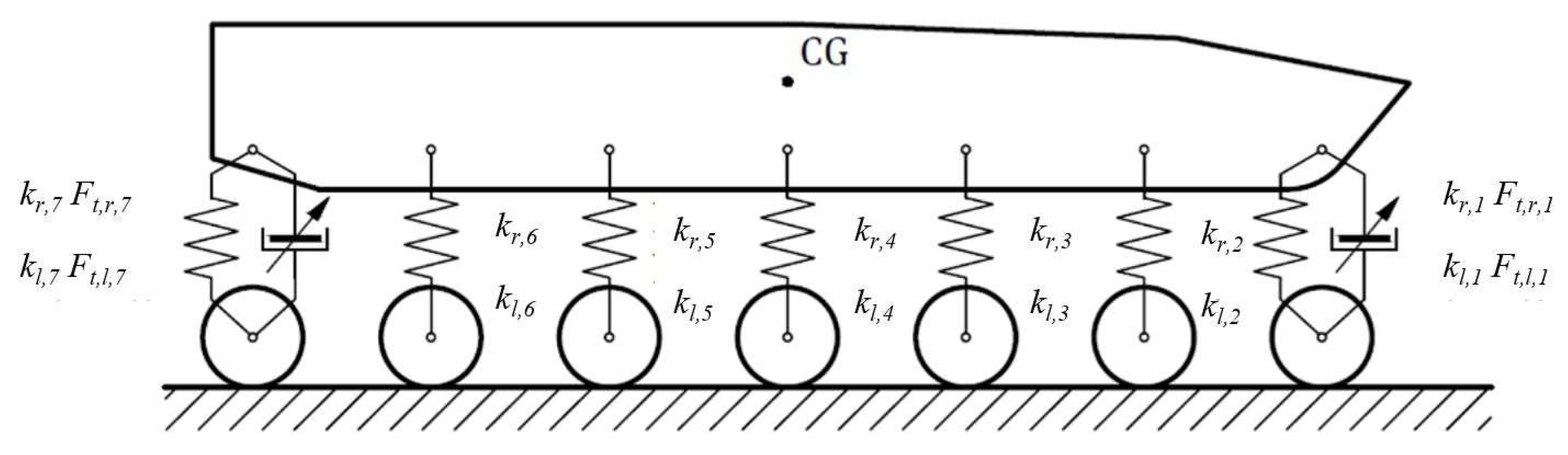
The discussions presented in the paper are based on the 2S1 platform suspension model shown in Figure 1. It consists of 14 packages of logarithmic spiral springs and 4 MR dampers. The MR dampers are located in the first and seventh axes. For instance, $F_{t,r,1}$ means that this is the force generated by the MR damper on the right side of the body in the first axis.

The following assumptions were made for the numerical analysis. It was assumed that temperature does not affect the magnetorheological fluid properties and that there is no leak of this fluid. Similar assumptions have been made for packages of logarithmic spiral springs. There is no oil temperature influence on the stiffness characteristics of the packages. The vehicle body can move in the vertical direction. It can also rotate around the center of gravity (CG). Linear stiffness and linear damping of road wheels were assumed. Furthermore, bilateral constraints were assumed. This means that road wheels always have contact with the substrate.

2.2. Continuous Skyhook Control Law for a Suspension System with Linear Stiffness Elements

The skyhook control law was proposed by Karnopp et al. in [19]. The application of the skyhook control law in the suspension system leads, among others, to the improvement of the ride comfort of the vehicle crew. This control law is the most commonly used in modern semi-active suspension systems of cars. Some examples of applications are presented in works [31,32]. In recent years, there has been a revelation of interest in this control law in the field of rail vehicle suspension systems [33]. In addition, the implementation of this control law in combat vehicles has been considered for several years. It is possible to indicate the work of [34] in which the authors analyzed a semi-active suspension system of a multi-wheeled combat vehicle with the skyhook control law. In work [35], the authors considered a simplified variant of the skyhook control law in the physical model of the suspension system of a 2S1 combat tracked vehicle created using the MSC Adams software. Nowadays, there is a wide range of suspension systems in which the discussed control law is considered.

The skyhook control law is based on a theoretical model in which it is assumed that the passive and linear viscous damper is combined with the sprung mass and an imaginary “sky.” This configuration reduces the amplitudes of displacement, velocity, and acceleration of the sprung mass, improving the ride comfort of the vehicle crew. The concept of the skyhook damper due to the fictitious viscous element is not physically realizable. In order to implement this control strategy, it is necessary to use an element with a controlled damping force value. This element can be placed between the sprung and unsprung mass, and the control signal of the actuator is proportional to the absolute velocity of the sprung mass, thus simulating Skyhook’s law. The MR damper actuator can be used in this function. Vibration systems in which magnetorheological dampers are used have feedback and require an external power supply. However, magnetorheological dampers are characterized by low power consumption and short response time to changes in the value of the electric current signal flowing through the control coils. Control of elements such as magnetorheological dampers is not the easiest one, due to their nonlinear characteristics.

Another continuous skyhook control law is the research performed by Hyvärinen et al. in work [22]. In contrast to the classical approach, it assumes the impact of three fictitious viscous dampers on the vehicle body. The first of these dampers is related to the vertical displacement of the sprung mass. The following two dampers are related to the pitch and roll of the vehicle body around its center of mass (CG). The first is the linear viscous damper, and the other two are rotational viscous dampers for calming pitch and roll. Those dampers should improve the ride comfort of the vehicle crew and vehicle body stability. For each of the fictitious dampers, it is assumed that their damping coefficients are critical damping coefficients of the vibrations. The critical damping coefficient in all three degrees of freedom must ensure the possibility of returning to the equilibrium without oscillation and in the shortest possible time.

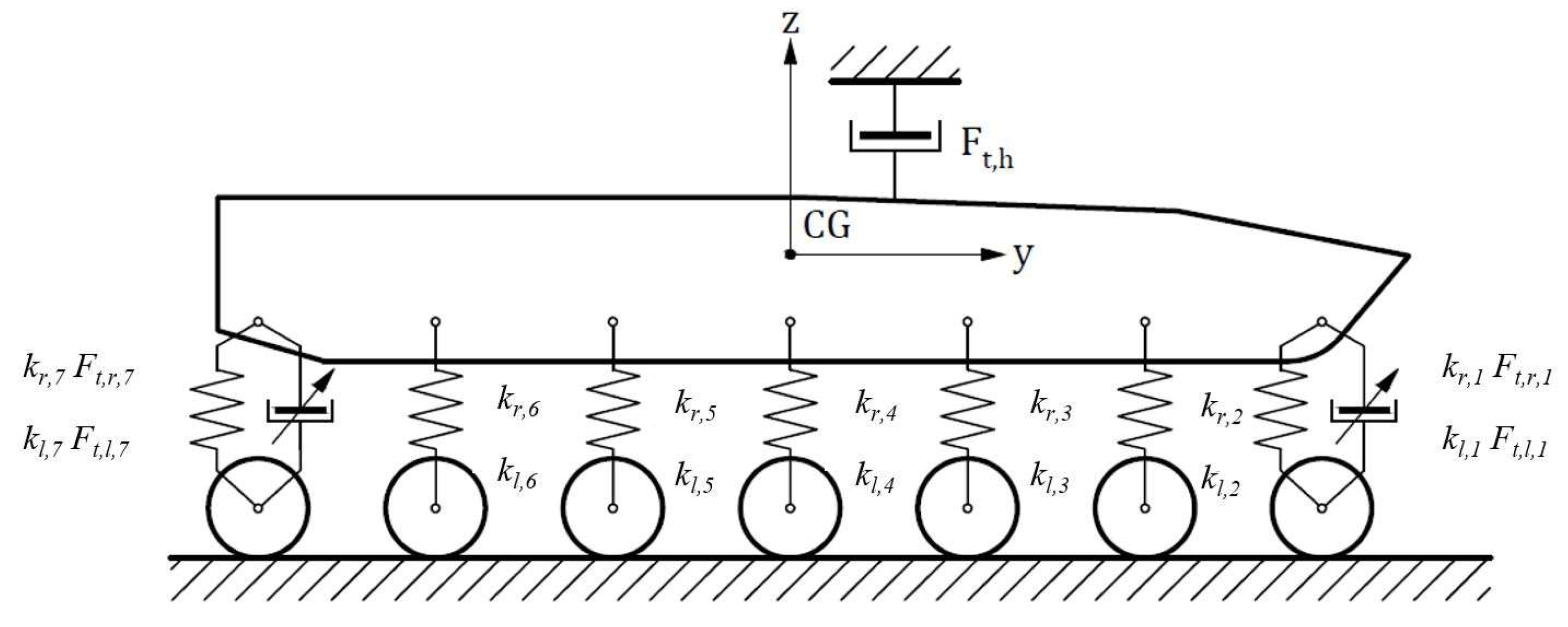
In the first stage of formulating the continuous skyhook control law, the linear viscous damper is connected with the sprung mass and an imaginary “sky.” This situation is presented in Figure 2.

The critical damping coefficient for the adopted model has the following form:

$$b_{h.cr}=2\sqrt{m_h\left({\displaystyle \sum }_{i=1}^7{k}_{r,i}+{\displaystyle \sum }_{i=1}^7{k}_{l, i}\right)}$$

(5)

For simplicity, the overall stiffness was calculated by Equations (6) and (7):

$${\overline{k}}_r={\displaystyle \sum }_{i=1}^7{k}_{r,i}$$

(6)

$${\overline{k}}_l={\displaystyle \sum }_{i=1}^7{k}_{l,i}$$

(7)

Thus, the force generated by the linear viscous damper connecting the center of mass (CG) of the vehicle body with an imaginary “sky” can be defined as follows:

$$F_{t,h}={\xi }_{h,sky}{b}_{h.cr}\dot{z}=2{\xi }_{h,sky}\sqrt{m_h\left({\overline{k}}_r+{\overline{k}}_l\right)}\dot{z}$$

(8)

The parameter ${\xi }_{h,sky}$ is a dimensionless quantity that, in the case of critical damping, is equal to 1. The force $F_{t,h}$ is still virtual. To make it real, it is assumed that this force is equal to the sum of damping forces generated by four MR dampers of the model. Thus, the following equation can be formulated:

$$F_{t,h}=F_{t,r,1}+F_{t,r,7}+F_{t,l,1}+F_{t,l,7}$$

(9)

The above equation contains four unknown variables. These unknown variables are damping forces $F_{t,r,1}$, $F_{t,r,7}$, $F_{t,l,1}$, and $F_{t,l,7}$. Successive equations have been formulated to find these values.

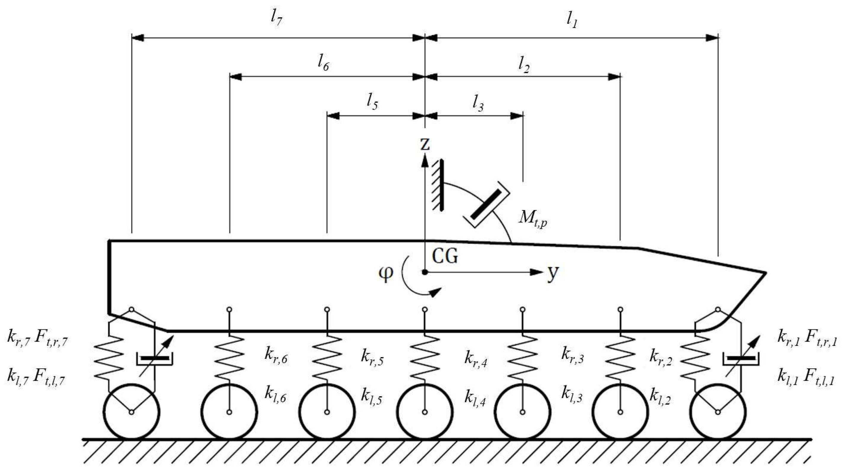
In the next stage of formulating the continuous skyhook control law, another fictitious viscous damper is added. This time, this is the virtual rotational viscous damper for pitch. The body rotates around the center of mass (CG). The following Figure 3 is relevant for the pitch of the body movement.

It is assumed that the fictitious rotational viscous damper generates the damping moment proportional to the angular velocity of the pitch. The critical damping coefficient is the proportionality factor in the equation. The rotation to the equilibrium should take the shortest possible time. The damping moment can be calculated as follows:

$$M_{t,p}={\xi }_{p,sky}{b}_{p,cr}\dot{\phi }=2{\xi }_{p,sky}\sqrt{J_x\left({\displaystyle \sum }_{i=1}^7{k}_{r,i}{l}_i^2+{\displaystyle \sum }_{i=1}^7{k}_{l,i}{l}_i^2\right)}\dot{\phi }$$

(10)

Similar to (6) and (7), the overall moments were calculated by Equations (11) and (12):

$${\overline{M}}_r={\displaystyle \sum }_{i=1}^7{k}_{r,i}{l}_i^2$$

(11)

$${\overline{M}}_l={\displaystyle \sum }_{i=1}^7{k}_{l,i}{l}_i^2$$

(12)

The parameter ${\xi }_{p,sky}$ is equal to 1 in the case of critical damping. It is assumed that all magnetorheological dampers of the model generate the damping moment. Thus, Equation (13) can be formulated as:

$$M_{t,p}=-F_{t,r,1}{l}_1+F_{t,r,7}{l}_7-F_{t,l,1}{l}_1+F_{t,l,7}{l}_7$$

(13)

Equations (9) and (13) are two of four equations that can be used to compute the damping forces $F_{t,r,1}$, $F_{t,r,7}$, $F_{t,l,1}$, and $F_{t,l,7}$ of MR dampers.

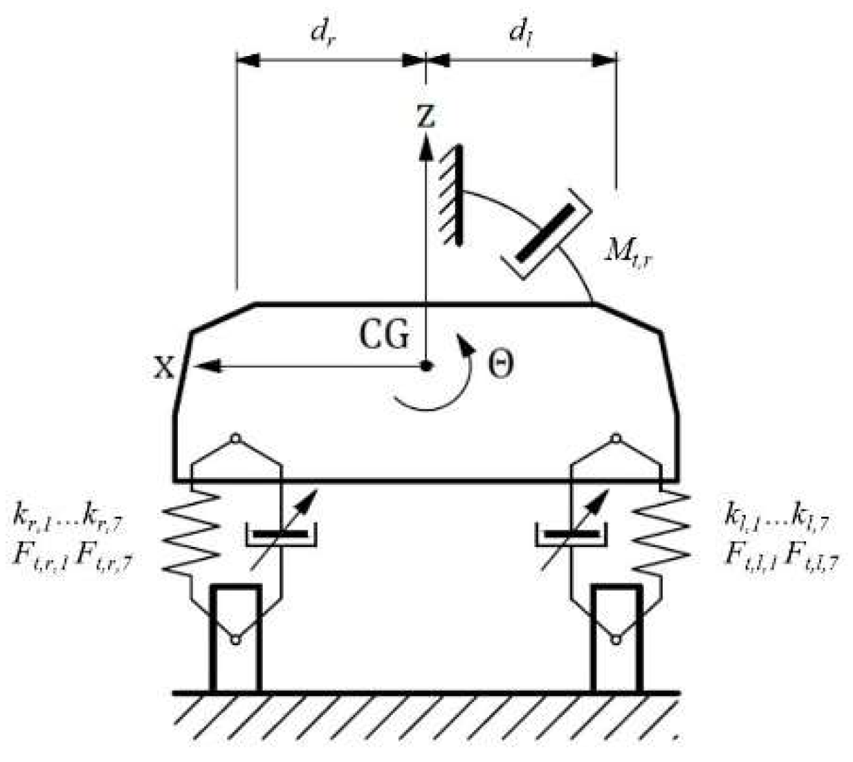
In the third stage, another viscous damper is added to the model Figure 4—this is the fictitious rotational viscous damper relevant for the body rolling movement.

The damping moment $M_{t,r}$ is proportional to the angular velocity of the roll. It is assumed that the damping coefficient of the fictitious rotational viscous damper should be the critical damping coefficient. In such a situation, the return to the equilibrium occurs without oscillation and in the shortest possible time. This should improve vehicle body stability. Given the above, the damping moment $M_{t,r}$ can be expressed as:

$$M_{t,r}={\xi }_{r,sky}{b}_{r,cr}\dot{\theta }=2{\xi }_{r,sky}\sqrt{J_y\left(d_r^2{\overline{k}}_r+d_l^2{\overline{k}}_l\right)}\dot{\theta }$$

(14)

As before, the damping ratio ${\xi }_{r,sky}$ in the case of critical damping is equal to 1. It is assumed that the generated damping moment $M_{t,r}$ is obtained by all MR dampers of the model. Therefore, the following equation can be written:

$$M_{t,r}=F_{t,r,1}{d}_r+F_{t,r,7}{d}_r-F_{t,l,1}{d}_l-F_{t,l,7}{d}_l$$

(15)

Equation (15) is the third in the system of four linear equations. It is necessary to enter one more equation to compute the damping forces of MR dampers. This equation is associated with body torsion. This equation can be written as:

$$T=-F_{t,r,1}{d}_r+F_{t,r,7}{d}_r+F_{t,l,1}{d}_l-F_{t,l,7}{d}_l$$

(16)

As the vehicle body is rigid and does not twist, the sum of the clockwise and anticlockwise moments $T$ is equal to 0. Thus, Equation (16) can be written as follows:

$$0=-F_{t,r,1}{d}_r+F_{t,r,7}{d}_r+F_{t,l,1}{d}_l-F_{t,l,7}{d}_l$$

(17)

Now, it is possible to determine the system of four linear equations. Based on Equations (9), (13), (15), and (17), the system of four linear equations takes the form (18):

$$\{\begin{array}{l}2{\xi }_{h,sky}\sqrt{m_h\left({\overline{k}}_r+{\overline{k}}_l\right)}\dot{z}=F_{t,r,1}+F_{t,r,7}+F_{t,l,1}+F_{t,l,7}\\ 2{\xi }_{p,sky}\sqrt{J_x\left({\overline{M}}_r+{\overline{M}}_l\right)}\dot{\phi }=-F_{t,r,1}{l}_1+F_{t,r,7}{l}_7-F_{t,l,1}{l}_1+F_{t,l,7}{l}_7\\ 2{\xi }_{r,sky}\sqrt{J_y\left(d_r^2{\overline{k}}_r+d_l^2{\overline{k}}_l\right)}\dot{\theta }=F_{t,r,1}{d}_r+F_{t,r,7}{d}_r-F_{t,l,1}{d}_l-F_{t,l,7}{d}_l\\ 0=-F_{t,r,1}{d}_r+F_{t,r,7}{d}_r+F_{t,l,1}{d}_l-F_{t,l,7}{d}_l\end{array}$$

(18)

Values of damping forces $F_{t,r,1}$, $F_{t,r,7}$, $F_{t,l,1}$, and $F_{t,l,7}$ are unknown, but, based on the above system of equations, it can be shown that:

$$F_{t,r,1}=\frac{1}{d_r+d_l}\left[{\xi }_{r,sky}\sqrt{J_y\left(d_r^2{\overline{k}}_r+d_l^2{\overline{k}}_l\right)}\dot{\theta }-\frac{2{\xi }_{p,sky}{d}_l}{l_1+l_7}\sqrt{J_x\left({\overline{M}}_r+{\overline{M}}_l\right)}\dot{\phi }+\frac{2{\xi }_{h,sky}{l}_7{d}_l}{l_1+l_7}\sqrt{m_h\left({\overline{k}}_r+{\overline{k}}_l\right)}\dot{z}\right]$$

(19)

For clarity of presentation in the main parts of the paper, only consideration for the first right axes is presented. The equations and figures for other axes corresponding with $F_{t,r,1}$ (19) are introduced in the Appendix A.

Equations (19) and (A1)–(A3) describe the continuous skyhook control law. This law can be applied to those suspension systems in which the stiffness elements have a linear characteristic.

2.3. Modification of Continuous Skyhook Control Law for a Suspension System with Nonlinear Stiffness Elements

The considered suspension system of the combat tracked vehicle in its structure contains 14 packages of logarithmic spiral springs. The force versus stroke characteristic of those elements is nonlinear [23]. Based on this observation, it is assumed that the stiffness coefficient of each package should be calculated as the slope of the tangent line to the nonlinear stiffness characteristic at the point in which the coordinate of abscissa is equal to the current value of the suspension deflection in a given suspension element. The considered suspension system of the combat tracked vehicle in its structure contains 14 packages of logarithmic spiral springs. The stiffness characteristic of those elements is nonlinear. Based on this observation, it is assumed that the stiffness coefficient of each package should be calculated as the slope of the tangent line to the nonlinear stiffness characteristic at the point in which the coordinate of abscissa is equal to the current value of the suspension deflection. Based on Equation (1), it can be calculated that the stiffness coefficient of the spring equals:

$$k={\left[\frac{\partial F_s\left(P,{\dot{z}}_w,z_w\right)}{\partial z_w}\right]}_{z_{wz}}={\left[5{\widehat{p}}_1{z}_w^4+3{\widehat{p}}_2{z}_w^2+{\widehat{p}}_3+sign\left({\dot{z}}_w\right)\left({\widehat{q}}_{1}P+{\widehat{q}}_2\right)\right]}_{z_{wz}}$$

(20)

The overall stiffness and moments generated by the force coming from logarithmic spiral springs were calculated by substitutions (21)–(24):

$${\overline{k}}_{\dot{F},r}={\displaystyle \sum }_{i=1}^7{\left(\frac{\partial F_s}{\partial z_w}\right)}_{z_{wz,r,i}}$$

(21)

$${\overline{k}}_{\dot{F},l}={\displaystyle \sum }_{i=1}^7{\left(\frac{\partial F_s}{\partial z_w}\right)}_{z_{wz,l,i}}$$

(22)

$${\overline{M}}_{\dot{F},r}={\displaystyle \sum }_{i=1}^7{\left(\frac{\partial F_s}{\partial z_w}\right)}_{z_{wz,r,i}}{l}_i^2$$

(23)

$${\overline{M}}_{\dot{F},l}={\displaystyle \sum }_{i=1}^7{\left(\frac{\partial F_s}{\partial z_w}\right)}_{z_{wz,l,i}}{l}_i^2$$

(24)

The application of the above notation to the stiffness coefficients in Equations (19) and (A1)–(A3) leads to new control law. This law is addressed to suspension systems employing linear spring characteristics. This law is still called the continuous skyhook control law. New equations are the effect of the application of the above formula in Equations (19) and (A1)–(A3). After substitutions, these equations take the form:

$$F_{t,r,1}=\frac{1}{d_r+d_l}\left[{\xi }_{r,sky}\sqrt{J_y\left(d_r^2{\overline{k}}_{\dot{F},r}+d_l^2{\overline{k}}_{\dot{F},l}\right)}\dot{\theta }-\frac{2{\xi }_{p,sky}{d}_l}{l_1+l_7}\sqrt{J_x\left({\overline{M}}_{\dot{F},r}+{\overline{M}}_{\dot{F},l}\right)}\dot{\phi }+\frac{2{\xi }_{h,sky}{l}_7{d}_l}{l_1+l_7}\sqrt{m_h\left({\overline{k}}_{\dot{F},r}+{\overline{k}}_{\dot{F},l}\right)}\dot{z}\right]$$

(25)

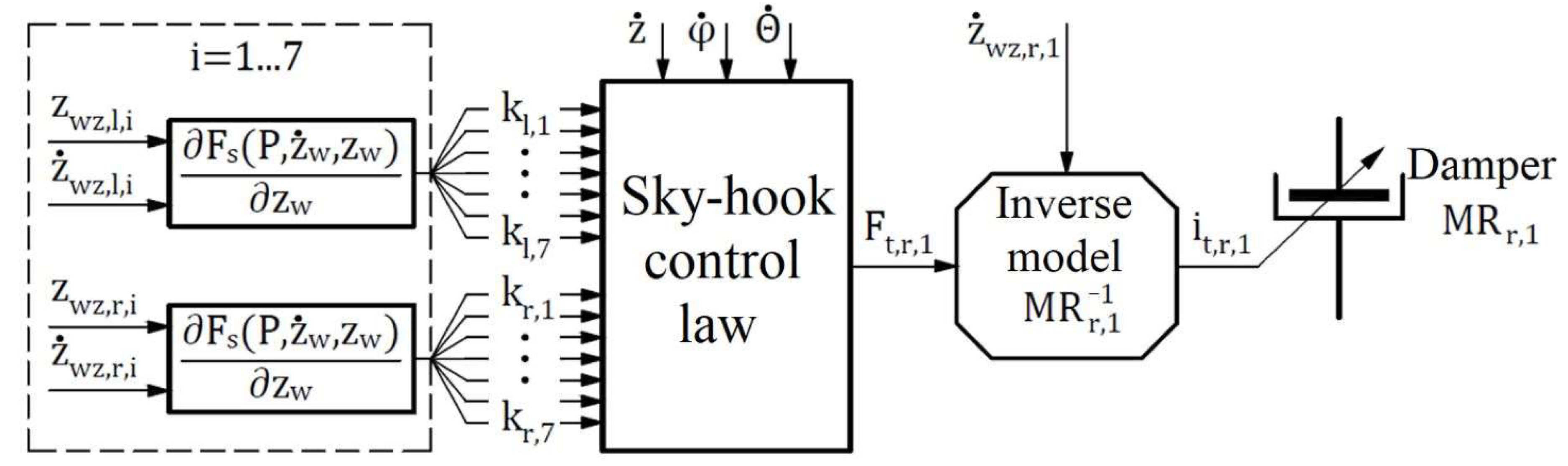
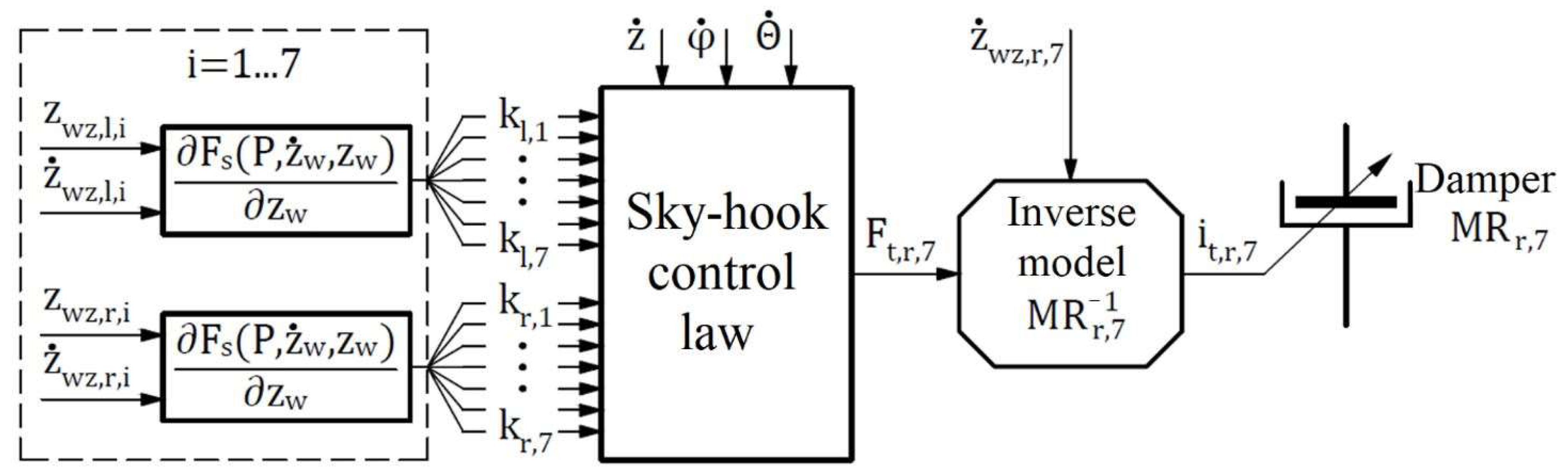
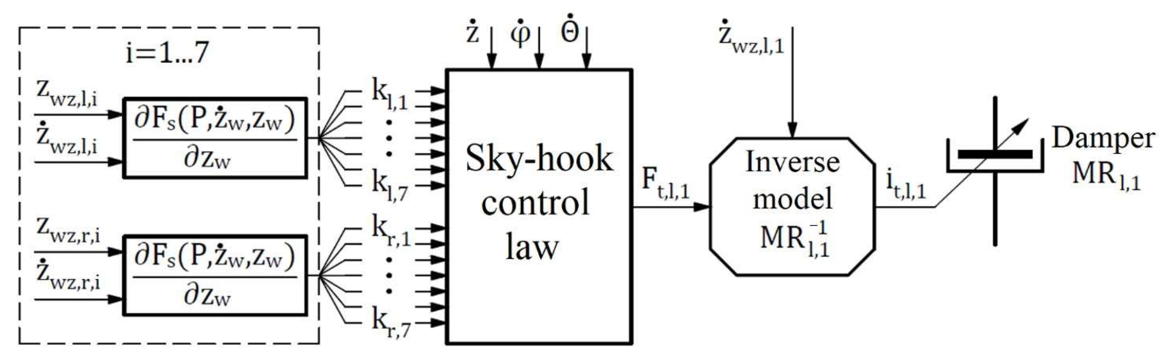
To obtain controlled values of damping forces $F_{t,r,1}$, $F_{t,r,7}$, $F_{t,l,1}$, and $F_{t,l,7}$ according to Equations (25) and (A4)–(A6), the authors propose the use of MR dampers. The damping force generated by these elements can be controlled depending on the magnetic field produced by a given current in the coils. The used mathematical model of the magnetorheological damper is the Bingham model. According to continuous skyhook control law, the current signals must have strictly defined values to achieve the damping forces. It is, therefore, necessary to introduce an inverse model of the MR damper [36]. The inverse model, according to Equation (2), has the form:

$$\begin{array}{l}{i}_t\left(F_t\right)=\frac{1}{2\left(a_{1}sign\left({\dot{z}}_{wz}\right)+c_1{\dot{z}}_{wz}\right)}\{[{\left(a_{2}sign\left({\dot{z}}_{wz}\right)+c_2{\dot{z}}_{wz}\right)}^2\\ -4\left(a_{1}sign\left({\dot{z}}_{wz}\right)+c_1{\dot{z}}_{wz}\right)\left(a_{3}sign\left({\dot{z}}_{wz}\right)+c_3{\dot{z}}_{wz}-F_t\right){]}^{\frac{1}{2}}-\left(a_{2}sign\left({\dot{z}}_{wz}\right)+c_2{\dot{z}}_{wz}\right)\}\end{array}$$

(26)

To obtain desired damping forces $F_{t,r,1}$, $F_{t,r,7}$, $F_{t,l,1}$, and $F_{t,l,7}$, it is necessary to use four independent inverse models of MR dampers. These models provide the values of current intensity signals $i_{t,r,1}$, $i_{t,r,7}$, $i_{t,l,1}$, and $i_{t,l,7}$. The use of Equation (26) for Equations (25) and (A4)–(A6) results in:

$$\begin{array}{l}{i}_{t,r,1}=\frac{1}{2\left(a_{1}sign\left({\dot{z}}_{wz,r,1}\right)+c_1{\dot{z}}_{wz,r,1}\right)}\left\{\right[{\left(a_{2}sign\left({\dot{z}}_{wz,r,1}\right)+c_2{\dot{z}}_{wz,r,1}\right)}^2\\ -4\left(a_{1}sign\left({\dot{z}}_{wz,r,1}\right)+c_1{\dot{z}}_{wz,r,1}\right)(a_{3}sign\left({\dot{z}}_{wz,r,1}\right)+c_3{\dot{z}}_{wz,r,1}\\ -\frac{1}{d_r+d_l}({\xi }_{r,sky}\sqrt{J_y\left(d_r^2{\overline{k}}_{\dot{F},r}+d_l^2{\overline{k}}_{\dot{F},l}\right)}\dot{\theta }-\frac{2{\xi }_{p,sky}{d}_l}{l_1+l_7}\sqrt{J_x\left({\overline{M}}_{\dot{F},r}+{\overline{M}}_{\dot{F},l}\right)}\dot{\phi }\\ +\frac{2{\xi }_{h,sky}{l}_7{d}_l}{l_1+l_7}\sqrt{m_h\left({\overline{k}}_{\dot{F},r}+{\overline{k}}_{\dot{F},l}\right)}\dot{z}\left)\right){]}^{\frac{1}{2}}-\left(a_{2}sign\left({\dot{z}}_{wz,r,1}\right)+c_2{\dot{z}}_{wz,r,1}\right)\}\end{array}$$

(27)

For clarity of presentation, similar control laws for other axes are presented in the Appendix A.

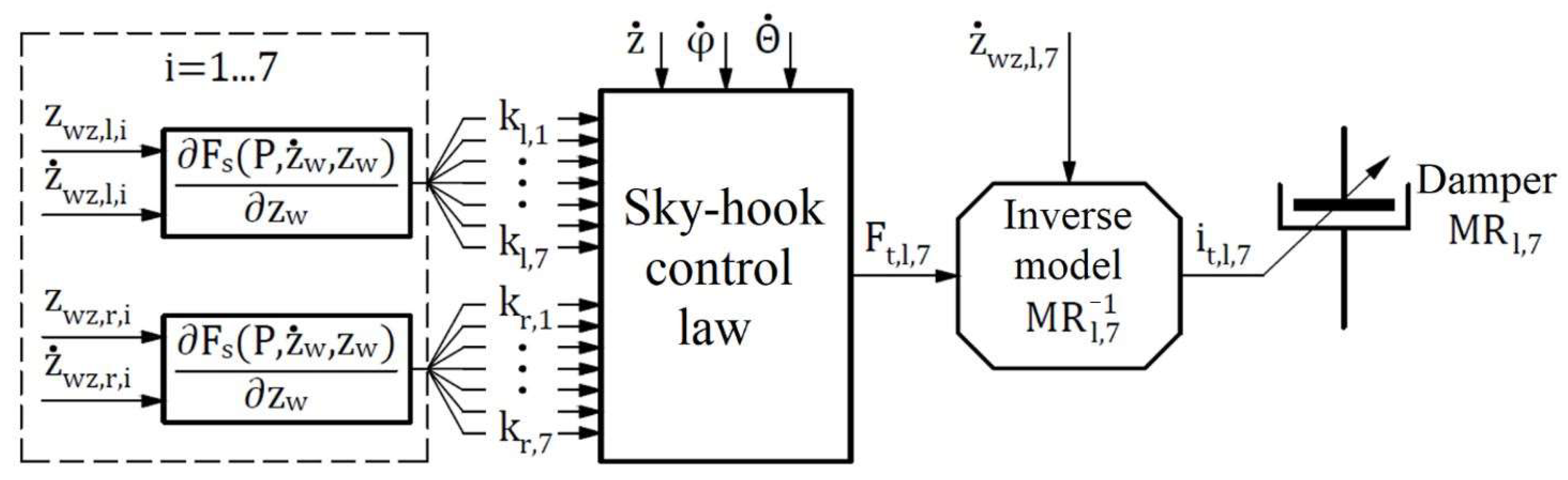
Equations (27) and (A9) and Figure 5 and Figure A1, Figure A2 and Figure A3 indicate that the algorithm for generating current signals $i_{t,r,1}$, $i_{t,r,7}$, $i_{t,l,1}$, and $i_{t,l,7}$ are carried out in successive stages. First, the stiffness coefficients are calculated—this is carried out based on Equation (20). The calculation proceeds for each of the 14 packages of logarithmic spiral springs. This stage is a common part of the calculation for each MR damper. Then, the damping forces $F_{t,r,1}$, $F_{t,r,7}$, $F_{t,l,1}$, and $F_{t,l,7}$ are calculated. Finally, current signals $i_{t,r,1}$, $i_{t,r,7}$, $i_{t,l,1}$, and $i_{t,l,7}$ are calculated based on inverse models of the Bingham model of the MR damper. The new continuous skyhook control law can be used for suspension systems with nonlinear stiffness elements. For numerical analysis, the authors assumed access to a complete state vector in which all coordinates can be measured. In reality, only limited measurements can be made. Therefore, unobserved state coordinates will be reconstructed with either a Luenberger or Kalman observer. Equations (27)–(29) and (A1)–(A9) are used in the numerical analysis.

3. Application

The modernization of the 2S1 tracked platform involves using packages of logarithmic spiral springs for each of the 14 road wheels. The package contains 15 logarithmic spiral springs. The thickness of a single spring is 3 mm. The logarithmic spiral springs are rotated relative to each other and are pre-compressed. There is friction between the springs. The spaces in the spring package were filled with oil to limit the temperature. Figure 6 shows the package of 15 logarithmic spiral springs.

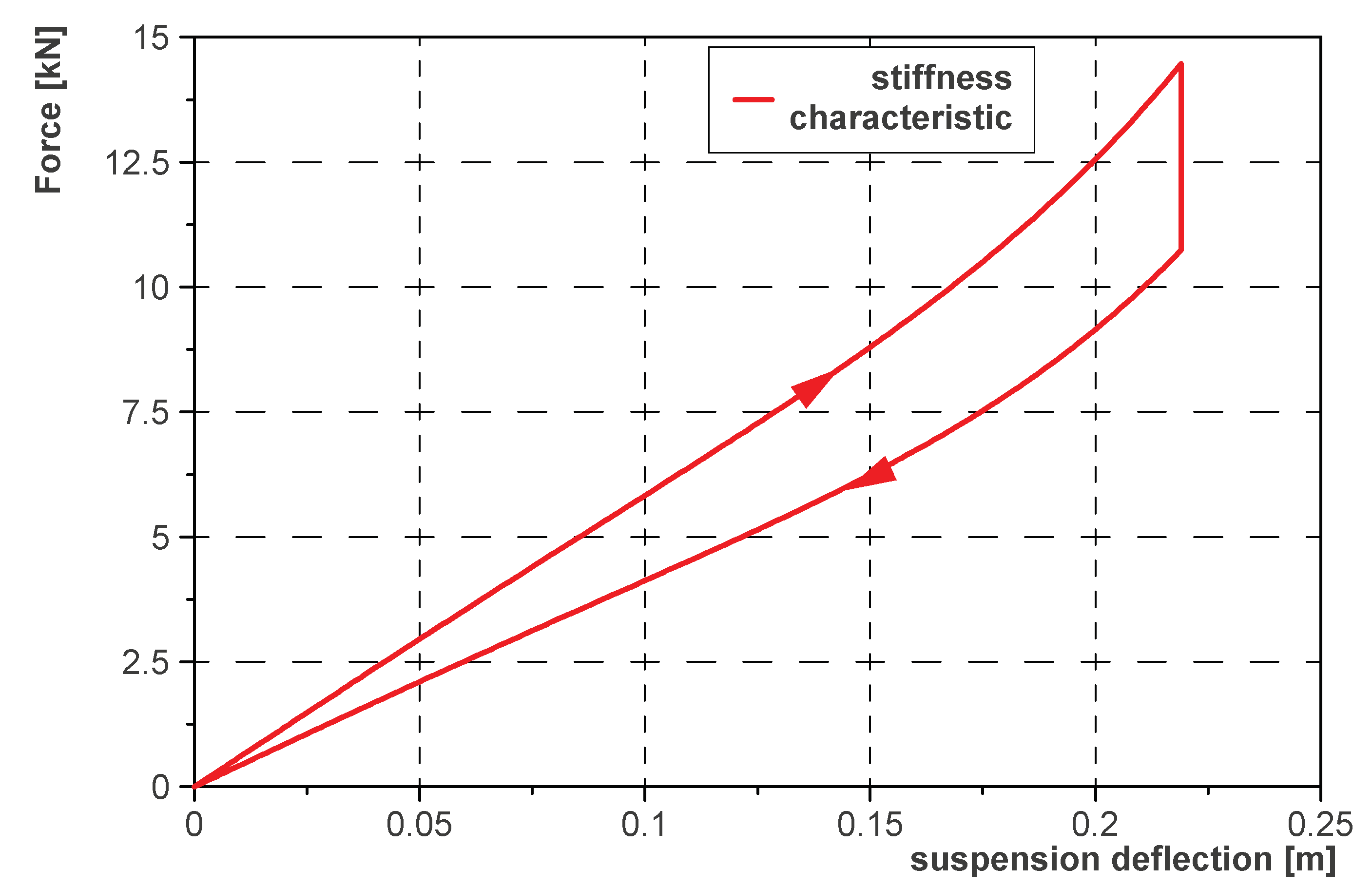
Figure 7 shows the stiffness characteristics obtained based on the measurement data for the proposed logarithmic spiral spring package. The upper curve was determined for the load increasing. On the other hand, the lower curve is the curve that was obtained for unloading the spring. In the tests, the packet deflection took place gradually, with breaks for stabilizing the measurement conditions. The result is the static characteristic determined when loading and unloading the spring. Tests were carried out for various oil pressures. With increasing pressure, the surface area between the loading and unloading curves decreased in subsequent experiments. This phenomenon is also taken into account by the mathematical model used. However, it is impossible to change the pressure in the package chassis while driving. Therefore, a constant pressure value of 0 (bar) was selected for the simulation. Figure 7 presents the stiffness characteristics when the oil pressure is equal to 0 bar.

4. Results and Discussion

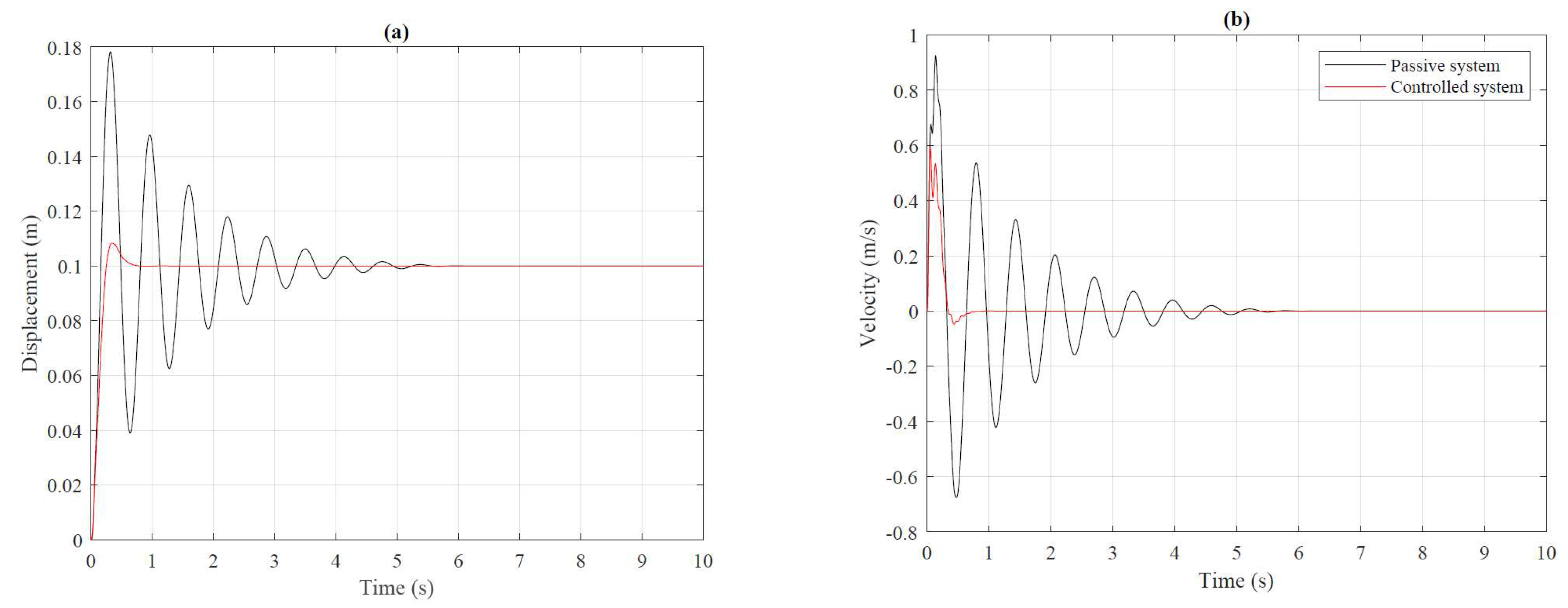
The time-domain analysis was carried out in the MATLAB environment MATLAB. (2020). version 9.9.0.1495850 (R2020b). Natick, MA: The MathWorks Inc. In the first stage, it was assumed that each road wheel was forced by the step signal with an amplitude of 0.1 m. For comparison purposes, the passive suspension system was examined too. In this case, values of electrical current signals generated in the coils of all MR dampers were set to 0 A. Next, the modified continuous skyhook control law was tested. The control law is defined by Equations (27) and (A1)–(A9). Figure 8 compares the vehicle body vertical displacement and vertical velocity for passive and controlled suspension. The velocity and displacement were measured in the center of mass (CG).

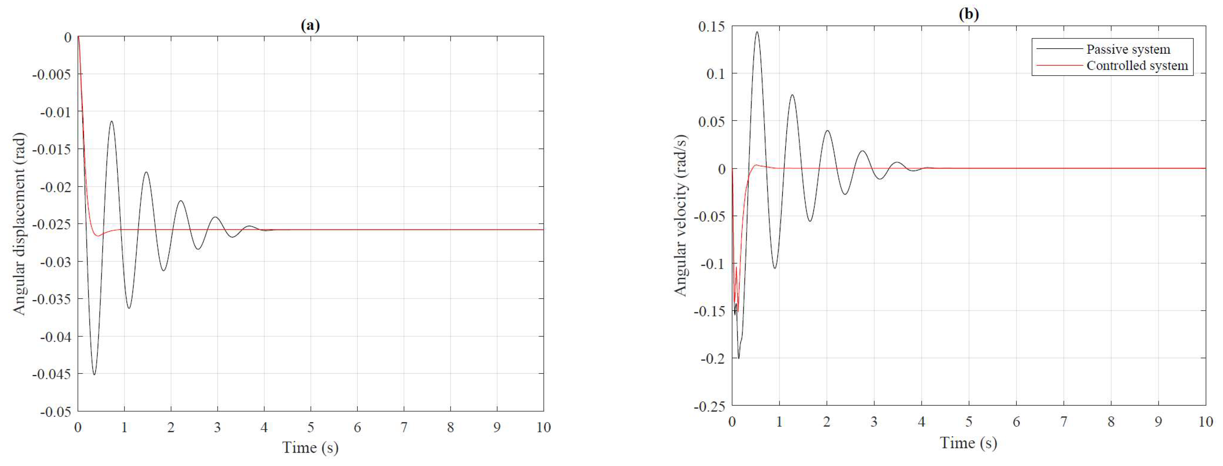
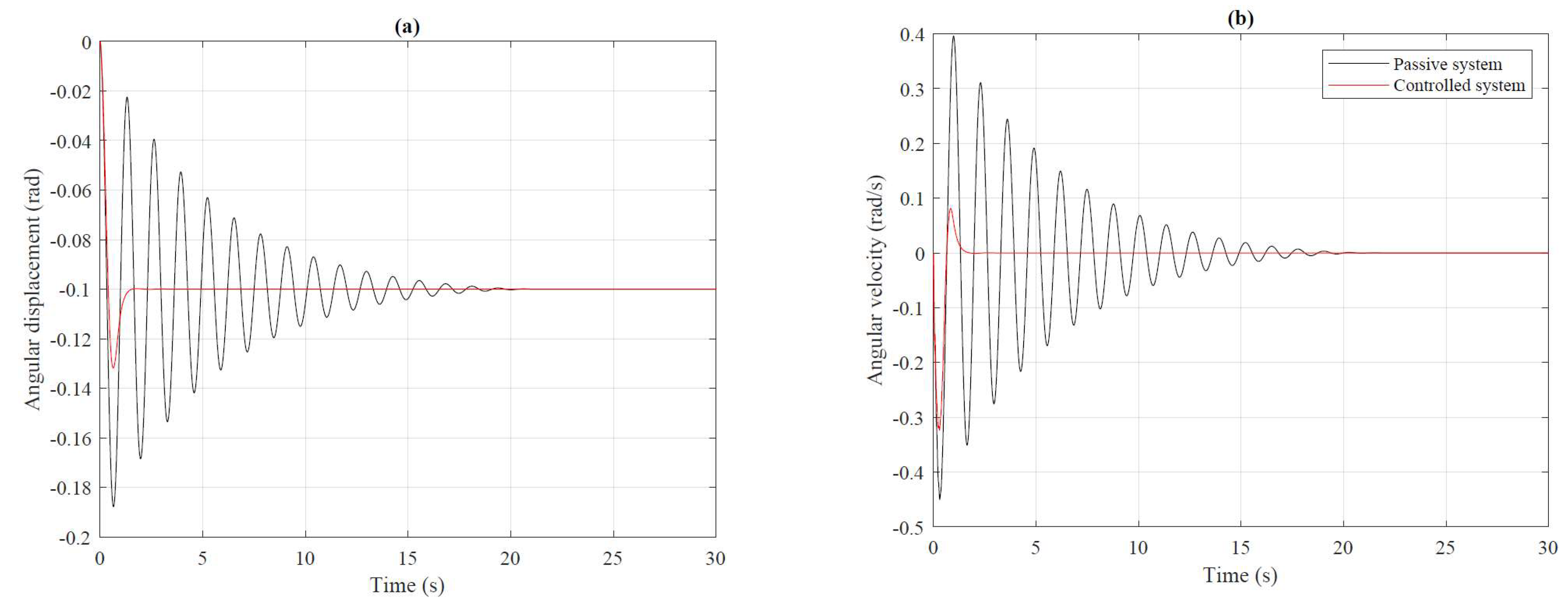
In the next stage, it was assumed that the first-axis road wheels were forced by the step signal with an amplitude of 0.1 m and the seventh-axis road wheels were forced by the step signal with an amplitude of −0.1 m. The angular displacement and angular velocity of the body moving around an axis running from left to right are presented in Figure 9.

A similar analysis was carried out for perpendicular direction along the rear-to-front axis of the vehicle (roll). This time, the road wheels were forced on the left and right sides of the body. The excitation signal was a step response of the amplitude of 0.1 m and −0.1 m, respectively. The results are shown in Figure 10.

Afterward, numerical analysis was performed using the well-known road profile of the Yuma proving ground. The numerical analysis assumed that the left side of the 2S1 tracked platform enters on an elevation with velocities of 12, 13, 14, 15, and 16 m/s. The selected obstacle had the shape of an equilateral triangle with a base length of 142 mm and a height of 71 mm. For each of the velocities of the 2S1 tracked platform, the root-mean-square index (RMS) and the maximum value of the vertical acceleration and angular accelerations were calculated. In addition, the exposure time was calculated for the whole chassis. For an individual wheel, the time in brackets is presented. The selected acceleration points were the same as above. The root-mean-square index (RMS) was calculated from Equation (28):

$$RMS=\sqrt{\frac{1}{N}{\displaystyle \sum }_{k=1}^N{a}_k^2}$$

(28)

The root-mean-square index (RMS) can also be used in the sensitivity study [37,38]. In this numerical analysis stage, the passive suspension system and the controlled suspension system were compared. The obtained data are summarized in

Table 2. The quality indicators of vertical acceleration of the vehicle body in the center of mass.

$\mathbf{Velocity} \left[\frac{\mathit{m}}{\mathit{S}}\right]$	Exposure Time [s]	Passive System		Controlled System
		$\mathbf{RMS} \left[\frac{\mathit{m}}{{\mathit{s}}^2}\right]$	${\mathit{A}}_{\mathit{m}\mathit{a}\mathit{x}}\left[\frac{\mathit{m}}{{\mathit{s}}^2}\right]$	$\mathbf{RMS} \left[\frac{\mathit{m}}{{\mathit{s}}^2}\right]$	${\mathit{A}}_{\mathit{m}\mathit{a}\mathit{x}}\left[\frac{\mathit{m}}{{\mathit{s}}^2}\right]$
12	0.50 (0.0828)	0.0734	0.4627	0.0727	0.4568
13	0.46 (0.0765)	0.0556	0.4319	0.0548	0.4274
14	0.43 (0.0710)	0.0453	0.4037	0.0442	0.4004
15	0.40 (0.0663)	0.0391	0.3821	0.0377	0.3795
16	0.37 (0.0621)	0.0356	0.3600	0.0340	0.3581

,

Table 3. The quality indicators of the angular acceleration for pitch angle.

$\mathbf{Velocity} \left[\frac{\mathit{m}}{\mathit{S}}\right]$	Exposure Time [s]	Passive System		Controlled System
		$\mathbf{RMS} \left[\frac{\mathit{m}}{{\mathit{s}}^2}\right]$	${\mathit{A}}_{\mathit{m}\mathit{a}\mathit{x}}\left[\frac{\mathit{m}}{{\mathit{s}}^2}\right]$	$\mathbf{RMS} \left[\frac{\mathit{m}}{{\mathit{s}}^2}\right]$	${\mathit{A}}_{\mathit{m}\mathit{a}\mathit{x}}\left[\frac{\mathit{m}}{{\mathit{s}}^2}\right]$
12	0.50 (0.0828)	0.0416	0.2853	0.0407	0.2849
13	0.46 (0.0765)	0.0330	0.2176	0.0320	0.2126
14	0.43 (0.0710)	0.0282	0.2126	0.0273	0.2041
15	0.40 (0.0663)	0.0253	0.2010	0.0245	0.1920
16	0.37 (0.0621)	0.0223	0.1785	0.0216	0.1696

and

Table 4. The quality indicators of angular acceleration for roll angle.

$\mathbf{Velocity} \left[\frac{\mathit{m}}{\mathit{S}}\right]$	Exposure Time [s]	Passive System		Controlled System
		$\mathbf{RMS} \left[\frac{\mathit{m}}{{\mathit{s}}^2}\right]$	${\mathit{A}}_{\mathit{m}\mathit{a}\mathit{x}}\left[\frac{\mathit{m}}{{\mathit{s}}^2}\right]$	$\mathbf{RMS} \left[\frac{\mathit{m}}{{\mathit{s}}^2}\right]$	${\mathit{A}}_{\mathit{m}\mathit{a}\mathit{x}}\left[\frac{\mathit{m}}{{\mathit{s}}^2}\right]$
12	0.50 (0.0828)	0.0185	0.0804	0.0177	0.0813
13	0.46 (0.0765)	0.0144	0.0651	0.0135	0.0643
14	0.43 (0.0710)	0.0119	0.0602	0.0110	0.0595
15	0.40 (0.0663)	0.0105	0.0567	0.0095	0.0561
16	0.37 (0.0621)	0.0096	0.0531	0.0087	0.0528

.

As one can see, Table 2, Table 3 and Table 4 indicate that the RMS values, as well as maximum acceleration value, are lower in the controlled suspension system than in the passive suspension system for each of the velocities.

After time domain studies, frequency domain analyses were performed. Three cases of vibration transmissibility characteristics were considered. All cases were delivered.

The sinusoidal signal was adopted to excite the wheels to imitate road roughness in all the considered cases. Such an excitation allowed for the determination of the vibration transmissibility function. The three cases included the following motion coordinates:

• $z$—displacement of the center of mass;
• $\phi$—pitch angle—where the vehicle’s front goes up or down about an axis running from wheel to wheel. Transverse tilting axis;
• $\theta$—roll angle—where the vehicle rotates about an axis running from rear to front of the car. Longitudinal tilting axis.

This approach evaluates the adopted quality indicators covering the ride comfort of the vehicle crew and vehicle body stability. For each of the three considered cases, the authors decided on five series of numerical experiments. As the 2S1 tracked platform has 14 road wheels and the assessment of the influence of each of them on the output coordinates is complicated, the authors considered the following cases of excitation:

• Excitation of the front axis (1) by sinusoidal signal—both wheels simultaneously $w_{l,1}=w_{r,1}=A·\sin \left(2·\pi ·f·t\right)$;
• Excitation of the front axis (1) by sinusoidal signal—delayed by $\pi /2$, right wheel in relation to the left wheel $w_{l,1}=A·sin\left(2·\pi ·f·t\right)$, $w_{r,1}=A·sin\left(2·\pi ·f·t+\pi /2\right)$;
• Excitation of the middle axis (4) by sinusoidal signal—both wheels simultaneously $w_{l,4}=w_{r,4}=A·sin\left(2·\pi ·f·t\right)$;
• Excitation of the rear axis (7) by sinusoidal signal—both wheels simultaneously $w_{l,7}=w_{r,7}=A·sin\left(2·\pi ·f·t\right)$;
• Excitation of the front (1) and rear (7) axis by sinusoidal signal delayed by $\pi /2$ relative to each other $w_{l,1}=w_{r,1}=A·sin\left(2·\pi ·f·t\right)$, $w_{l,7}= w_{r,7}=A·sin\left(2·\pi ·f·t+\pi /2\right)$.

The range of considered frequencies f was $0-15$ Hz. The amplitudes A of all kinematic excitations were $0.1$ m.

The vibration transmissibility characteristics were calculated as:

$$T_{y,w}=10log\left(\frac{{\int }_0^{T_f}{y}^{2}dt}{{\int }_0^{T_f}{w}^{2}dt}\right)$$

(29)

where $T_f—$the period of the excitation signal; $w$—the input signal (excitation); $y$—the output signal substituted by z, $\phi , \theta$, which is the center of the mass displacement, pitch angle, and roll angle, respectively. A constant value was removed from both signals.

During numerical analysis in the passive case, values of electrical current signals flowing through the coils of MR dampers were set to 0 A.

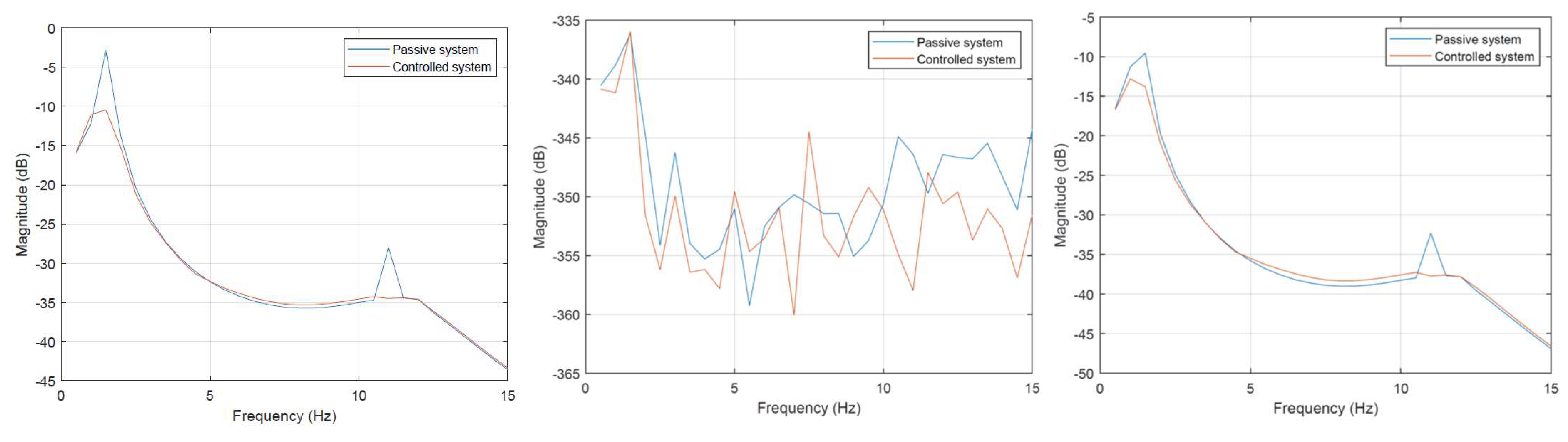
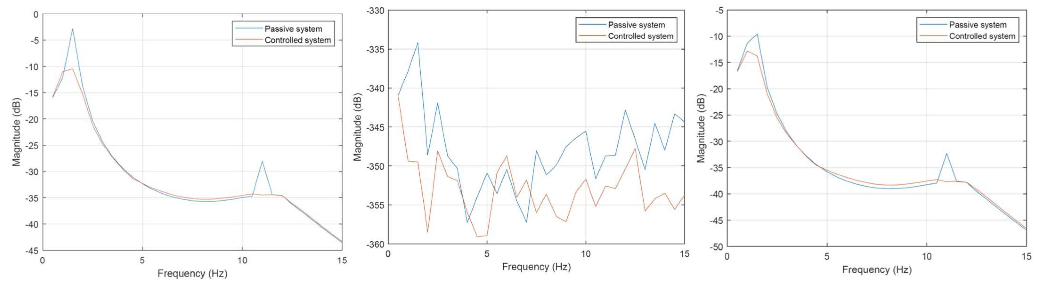
On the first test, the front road wheel of the 2S1 tracked platform was forced by the same sinusoidal signal. At this stage, the center of the mass displacement and both adopted angles were measured. It was performed for the controlled and passive cases. Equation (29) was used to compute the vibration transmissibility characteristics. The vibration transmissibility characteristics for all output cases, displacement of the center of mass, pitch angle, and roll angle are shown in Figure 11, respectively.

In Figure 11, the vehicle frequency response results show the reduction in vertical vibration and swaying in both angular directions. Vibration reduction of the mass center with respect to excitation results from the suspension ratio on the length $l_1$ (see Figure 3). Negative magnitude values over the entire frequency range, for pitch angle characteristics, result from comparing different coordinates units, in particular, the angle $\phi$ calculated in rad units and the displacement excitation calculated in m.

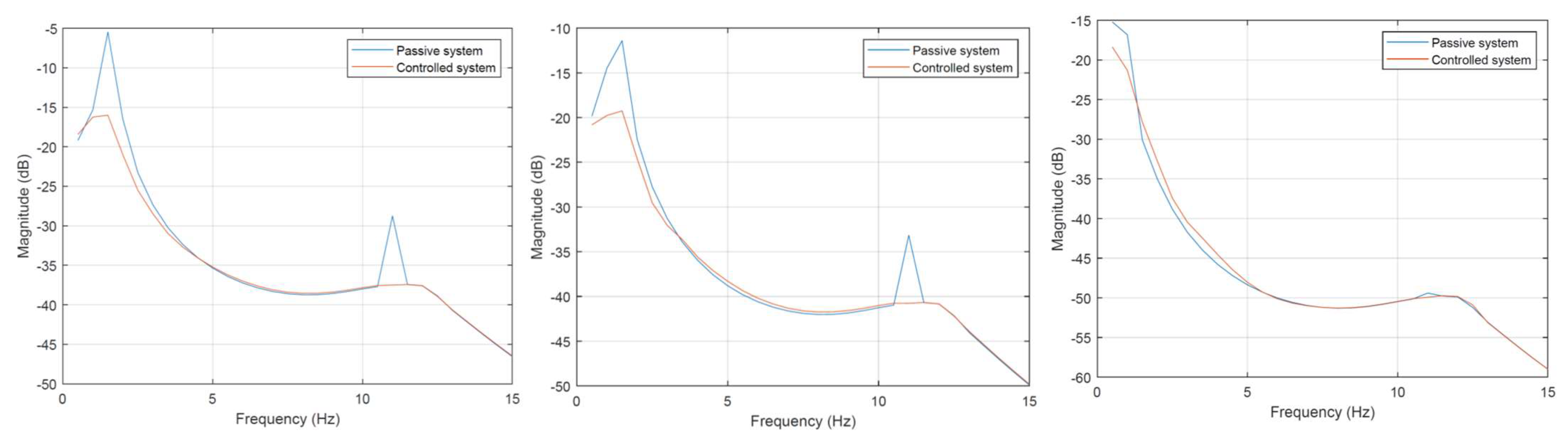
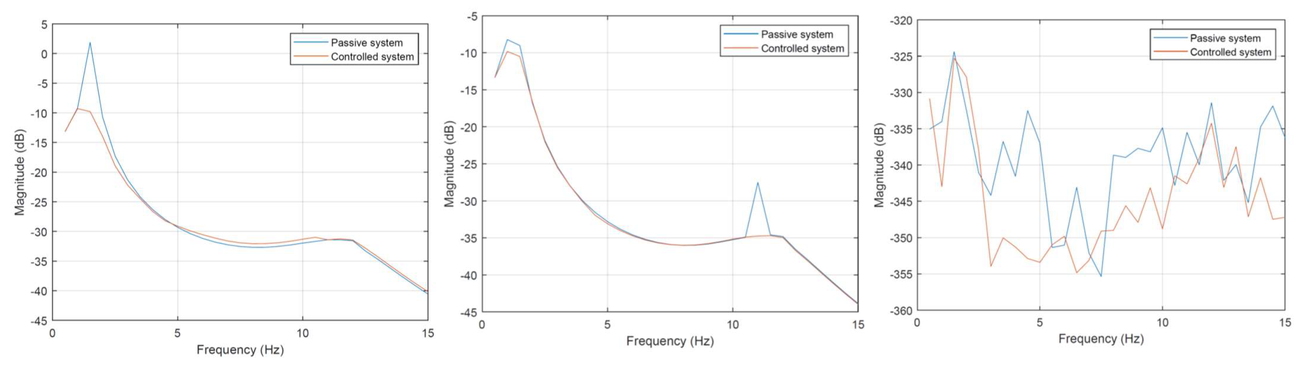
Similar effects, i.e., negative magnitude values, can be observed when analyzing the adopted motion coordinates with the asymmetric excitation of the front axis in Figure 12. In this figure, the most interesting case is the pitch angle transmissibility shown in the middle of Figure 12. As can be seen, the magnitude near both resonance frequencies is significantly reduced. On the right-hand side of the figure, one can see the influence of the front-axis asymmetric excitation on the roll angle. In this case, the reduction in vibrations results mainly from the geometry of the chassis. The significant distance of the front axis to the center of rotation $\theta$ has no influence on roll angle.

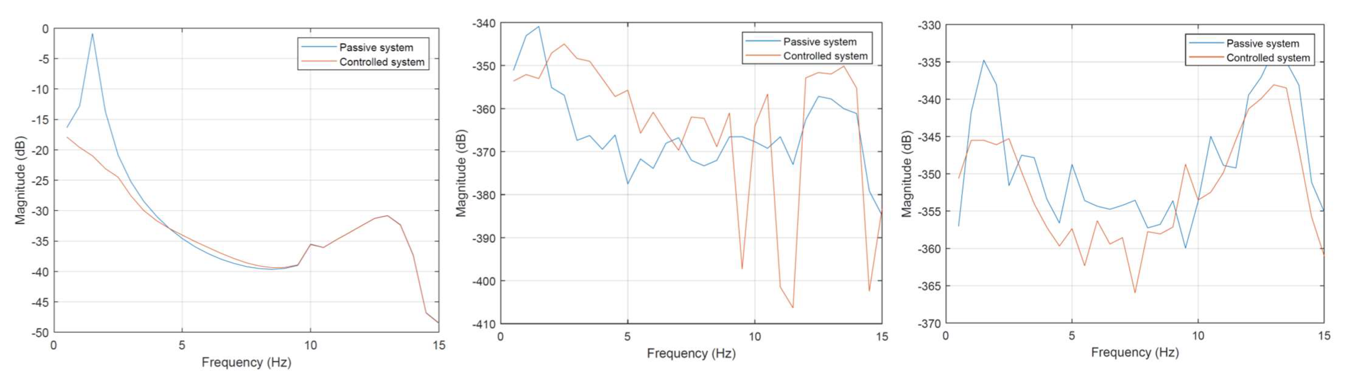
When we excite the central axis in Figure 13, the influence of disturbance on the reduction in vibrations is visible in the left figure, showing the displacement of the center of the mass vibration transmissibility. This excitation does not cause any pitch or roll angles vibration. As before, negative magnitude values are the result of the compared values units of rad and m.

In Figure 14, representing the rear axis excitation, all three characteristics are similar to those shown in Figure 11. This results from the assumed symmetrical weight distribution for 2S1 tracked platforms.

The vibration transmissibility characteristics shown in Figure 15 were obtained by excitation applied for the front and rear axis. The signals were delayed by $\pi /2$ to initiate vibrations about the transverse axis. Such an excitation causes the vehicle to raise the nose and lower the tail of the vehicle alternately. This excitation produces only transverse vibration, and no longitudinal vibrations are observed. This can be seen at the central and right characteristics of Figure 15. In the left figure characterizing the center of the mass displacement, it can be observed that no second resonance is visible for the passive system.

Discussion of the Numerical Investigation Results

Due to the fact that other research works have applied their considerations to objects with different parameters and structures, the main point of reference is the passive suspension.

The first stage concerned the determination of time charts. Analysis of Figure 8 and Figure 9 indicates the effectiveness of the modified continuous shy-hook control law. The oscillations of the presented signals are more significant in the passive system. There are no significant oscillations in a system where the modified continuous skyhook control law has been applied. The controlled system reaches the equilibrium point in a shorter time than the passive one.

Numerical analysis of the road profile from the Yuma proving ground—summarized in Table 2, Table 3 and Table 4—showed that the RMS values are lower in the controlled suspension system than in the passive suspension system for each of the velocities. This means that the amplitude of vertical and angular accelerations was reduced by employing the proposed control system application.

Independent of the front or rear axis, the excitation for both wheels simultaneously shows that the algorithm used reduces the amplitude of vibrations for both natural frequencies. Applied control methods allow the reduction in resonance and low energy consumption at the same time. The energy used results only from the control signal, improving comfort in the area of resonance. As can be seen, excitation of the front or rear axes does not affect the vibration of the longitudinal axis.

For Figure 11, Figure 12, Figure 13, Figure 14 and Figure 15, a more efficient reduction in vibrations can be observed surrounding the area of natural frequencies, i.e., 1.45 Hz and 10.9 Hz—this means that the algorithm proposed by the authors meets its goals.

The applied semi-active control system improves both the comfort and safety of passengers in relation to the passive system.

The semi-active suspension system will be used in the military 2S1 tracked platform. However, due to the significant improvement in ride comfort—proven later in the article—it can also be used in civil vehicles, e.g., designed to save people from endangered areas. The application of the modified continuous skyhook control law requires, inter alia, the measurement of the stiffness characteristics of the suspension spring element. Such tests were carried out due to the future use in a combat vehicle. The result of this measurement, among other things, is the stiffness characteristic presented in Figure 7.

5. Conclusions

The time-domain analysis indicates that the usage of the modified continuous skyhook control law reduces amplitudes of vertical displacement and vertical velocity of the center of gravity of the vehicle body and shortens the time needed to achieve the appropriate level. The system returns to the equilibrium point without large oscillations. The velocities of the vehicle center of gravity are lower in the controlled case than in the passive case. Thanks to the control application, the quality indicator responsible for driving comfort has been improved. The increase in the ride comfort of the vehicle crew improves the quality of soldiers’ work. Better comfort could mean the shortening of the reaction time and appropriate decision making. In the case of pitch and roll, it can be seen that the system tends to the equilibrium point faster. There is no large oscillation in the controlled case. In the passive case, oscillations are present. Angular velocities of pitch and roll have significantly lower values in the controlled case than in the passive case. The improvement of the vehicle body stability has been achieved. This improvement can positively affect the function of the main gun stabilizer, which means an increase in firing accuracy.

Data shown in Table 2, Table 3 and Table 4 indicate that the RMS index values are smaller in the controlled suspension system than in the passive suspension system. There is an improvement in the body stability and the ride comfort of the vehicle crew under the ride conditions in the Yuma proving ground. The reduction in RMS values with the increase in velocity of the 2S1 tracked platform confirms that the numerical analysis was carried out correctly. As the velocity increases, the impact of the obstacle is shorter. Therefore, the obtained results, which are an essential element of the time-domain analysis, are correct.

Frequency vibration transmissibility characteristics show that modifying the continuous skyhook control law is adequate. The transmissibility characteristics in natural frequencies of the vehicle body have significantly lower values when the continuous skyhook control law is modified. Good results of control law improvement mean that after hitting an obstacle, the vehicle body will return to the equilibrium point in a shorter time. The results of the frequency-domain analysis confirm the results of the time-domain analysis. The proposed modification of the continuous skyhook control law leads to the improvement of the vehicle body stability and the ride comfort of the vehicle crew.

The elimination of torsion bars from the tracked military platform in question is of key importance for modernized vehicles. The introduction of a new design of springs significantly reduces the dimensions but introduces nonlinearity. The calculation of the equivalent spring stiffness coefficient as the slope of the tangent to the nonlinear stiffness characteristic at the point where the abscissa is equal to the current value of the suspension deflection allows the use of the continuous skyhook control law. The use of controlled magnetorheological dampers enables the crew’s comfort and safety to be improved and to compensate for the disadvantages of using a nonlinear spring. After introducing appropriate mechanical modifications, the authors plan to apply the control law described in the article and conduct tests on the proving ground.

6. Patents

Patents granted in the territory of the Republic of Poland related to the research presented in the article.

• A vehicle suspension assembly, especially multi-wheel off-road vehicles;
• Inventors: M. Apostoł; A. Jurkiewicz; T. Cygankiewicz; J. Kowal; J. Konieczny; P. Micek; A. Rusinek; A. Matuła; J. Zając; T. Pieprzny.
• Application P.393407 events
• 2010-12-23 Application filed by AGH University of Science and Technology
• 2011-06-20 Publication of PL 393407 A1
• 2014-03-31 Publication of PL 216343 B1
• 2013-08-21 Application granted
• Status Active

• Hydraulic rotary actuator;
• Inventors: M. Apostoł; A. Jurkiewicz; T. Cygankiewicz; J. Kowal; J. Konieczny; P. Micek; A. Rusinek; A. Matuła; J. Zając; T. Pieprzny.
• Application P.393536 events
• 2010-12-31 Application filed by AGH University of Science and Technology
• 2011-06-20 Publication of PL 393536 A1
• 2014-02-28 Publication of PL 215934 B1
• 2013-06-26 Application granted
• Status Active

• Cumulative, flexible coupling;
• Inventors: M. Apostoł; A. Jurkiewicz; T. Cygankiewicz; J. Kowal; J. Konieczny; P. Micek; A. Rusinek; A. Matuła; J. Zając; T. Pieprzny.
• Application P.393537 events
• 2010-12-31 Application filed by AGH University of Science and Technology
• 2011-08-01 Publication of PL 393537 A1
• 2014-02-28 Publication of PL 216095 B1
• 2013-07-15 Application granted
• Status Active

References

- Morato, M.M.; Nguyen, M.Q.; Sename, O.; Dugard, L. Design of a fast real-time LPV model predictive control system for semi-active suspension control of a full vehicle. J. Frankl. Inst. 2019, 356, 1196–1224. [Google Scholar] [CrossRef]
- Ghoniem, M.; Awad, T.; Mokhiamar, O. Control of a new low-cost semi-active vehicle suspension system using artificial neural networks. Alex. Eng. J. 2020, 59, 4013–4025. [Google Scholar] [CrossRef]
- Pang, H.; Liu, F.; Xu, Z. Variable universe fuzzy control for vehicle semi-active suspension system with MR damper combining fuzzy neural network and particle swarm optimization. Neurocomputing 2018, 306, 130–140. [Google Scholar] [CrossRef]
- Ma, T.; Bi, F.; Wang, X.; Tian, C.; Lin, J.; Wang, J.; Pang, G. Optimized fuzzy skyhook control for semi-active vehicle suspension with new inverse model of magnetorheological fluid damper. Energies 2021, 14, 1674. [Google Scholar] [CrossRef]
- Aljarbouh, A.; Fayaz, M. Hybrid modelling and sliding mode control of semi-active suspension systems for both ride comfort and road-holding. Symmetry 2020, 12, 1286. [Google Scholar] [CrossRef]
- Konieczny, J.; Sibielak, M.; Rączka, W. Active vehicle suspension with anti-roll system based on advanced sliding mode controller. Energies 2020, 13, 5560. [Google Scholar] [CrossRef]
- Tudon-Martinez, J.C.; Hernandez-Alcantara, D.; Sename, O.; Morales-Menendez, R.; Lozoya-Santos, J.D.J. Parameter-dependent H∞ filter for LPV semi-active suspension systems. IFAC-PapersOnLine 2018, 51, 19–24. [Google Scholar] [CrossRef]
- Vela, A.E.; Alcántara, D.H.; Menendez, R.M.; Sename, O.; Dugard, L. H∞ observer for damper force in a semi-active suspension. IFAC-PapersOnLine 2018, 51, 764–769. [Google Scholar] [CrossRef]
- Sibielak, M.; Raczka, W.; Konieczny, J.; Kowal, J. Optimal control based on a modified quadratic performance index for systems disturbed by sinusoidal signals. Mech. Syst. Signal Process. 2015, 64–65, 498–519. [Google Scholar] [CrossRef]
- Konieczny, J.; Rączka, W.; Sibielak, M.; Kowal, J. Energy consumption of an active vehicle suspension with an optimal controller in the presence of sinusoidal excitations. Shock Vib. 2020, 2020, 6414352. [Google Scholar] [CrossRef]
- Liu, C.; Chen, L.; Yang, X.; Zhang, X.; Yang, Y. General theory of skyhook control and its application to semi-active suspension control strategy design. IEEE Access 2019, 7, 101552–101560. [Google Scholar] [CrossRef]
- Konieczny, J.; Kowal, J.; Raczka, W.; Sibielak, M. Bench tests of slow and full active suspensions in terms of energy consumption. J. Low Freq. Noise Vib. Act. Control 2013, 32, 81–98. [Google Scholar] [CrossRef]
- Sibielak, M.; Konieczny, J.; Kowal, J.; Raczka, W.; Marszalik, D. Optimal control of slow-active vehicle suspension—Results of experimental data. J. Low Freq. Noise Vib. Act. Control 2013, 32, 99–116. [Google Scholar] [CrossRef]
- Jurkiewicz, A.; Kowal, J.; Zając, K. Model studies of the modernized 2S1 tracked vehicle suspension system. In Proceedings of the 31st International Symposium on Science and Technology, Kraków, Poland, 27–28 October 2016; Nawrocka, A., Flaga, S., Eds.; Department of Process Control, Faculty of Mechanical Engineering and Robotics, AGH University of Science and Technology: Kraków, Poland, 2016. [Google Scholar]
- Jurkiewicz, A.; Kowal, J.; ZajĄc, K. Sky-hook control and Kalman filtering in nonlinear model of tracked vehicle suspension system. Acta Mech. Autom. 2017, 11, 222–228. [Google Scholar] [CrossRef] [Green Version]
- Jamroziak, K.; Kosobudzki, M.; Ptak, J. Assessment of the comfort of passenger transport in special purpose vehicles. Eksploat. Niezawodn. 2013, 15, 25–30. [Google Scholar]
- Burdzik, R.; Konieczny, Ł. Vibration issues in passenger car. Transp. Probl. 2014, 9, 83–90. [Google Scholar]
- Bajkowski, J.M. Design, analysis and performance evaluation of the linear, magnetorheological damper. Acta Mech. Autom. 2012, 6, 5–9. [Google Scholar]
- Karnopp, D.; Crosby, M.J.; Harwood, R.A. Vibration control using semi-active force generators. J. Manuf. Sci. Eng. Trans. ASME 1974, 96, 619–626. [Google Scholar] [CrossRef]
- Lam, A.H.F.; Liao, W.H. Semi-active control of automotive suspension systems with magneto-rheological dampers. Int. J. Veh. Des. 2003, 33, 50–75. [Google Scholar] [CrossRef]
- Simon, D.; Ahmadian, M. Vehicle evaluation of the performance of magneto rheological dampers for heavy truck suspensions. J. Vib. Acoust. Trans. ASME 2001, 123, 365–375. [Google Scholar] [CrossRef]
- Hyvärinen, J.-P. The Improvement of Full Vehicle Semi-Active Suspension through Kinematical Model; University of Oulu: Oulu, Finland, 2004; ISBN 9514276116. [Google Scholar]
- Nabagło, T.; Jurkiewicz, A.; Kowal, J. Modeling verification of an advanced torsional spring for tracked vehicle suspension in 2S1 vehicle model. Eng. Struct. 2021, 229, 111623. [Google Scholar] [CrossRef]
- Kciuk, M.; Turczyn, R. Properties and application of magnetorheological fluids. J. Achiev. Mater. Manuf. Eng. 2006, 18, 127–130. [Google Scholar]
- Qin, Y.; Xiang, C.; Wang, Z.; Dong, M. Road excitation classification for semi-active suspension system based on system response. J. Vib. Control 2018, 24, 2732–2748. [Google Scholar] [CrossRef]
- Wang, E.K.; Ma, X.Q.; Rakheja, S.; Su, C.Y. Semi-active control of vehicle vibration with MR-dampers. In Proceedings of the 42nd IEEE International Conference on Decision and Control (IEEE Cat. No. 03CH37475), Maui, HI, USA, 9–12 December 2003; Volume 3, pp. 2270–2275. [Google Scholar]
- Guo, S.; Yang, S.; Pan, C. Dynamic modeling of magnetorheological damper behaviors. J. Intell. Mater. Syst. Struct. 2006, 17, 3–14. [Google Scholar] [CrossRef]
- Hu, G.; Liu, Q.; Ding, R.; Li, G. Vibration control of semi-active suspension system with magnetorheological damper based on hyperbolic tangent model. Adv. Mech. Eng. 2017, 9, 1–15. [Google Scholar] [CrossRef]
- Sapiński, B.; Filuś, J. Analysis of parametric models of MR linear damper. J. Theor. Appl. Mech. 2003, 41, 215–240. [Google Scholar]
- Sapiński, B.; Jstrzębski, Ł.; Węgrzynowski, M. Modelling of a self-powered vibration reduction system. Model. Inżynierskie 2011, 10, 353–362. [Google Scholar]
- Yi, K.; Song, B.S. A new adaptive sky-hook control of vehicle semi-active suspensions. Proc. Inst. Mech. Eng. Part D J. Automob. Eng. 1999, 213, 293–303. [Google Scholar] [CrossRef]
- Gopala Rao, L.V.V.; Narayanan, S. Sky-hook control of nonlinear quarter car model traversing rough road matching performance of LQR control. J. Sound Vib. 2009, 323, 515–529. [Google Scholar] [CrossRef]
- Li, H.; Goodall, R.M. Linear and non-linear skyhook damping control laws for active railway suspensions. Control Eng. Pract. 1999, 7, 843–850. [Google Scholar] [CrossRef]
- Kciuk, S.; Duda, S.; Mężyk, A.; Świtoński, E.; Klarecki, K. Tuning the dynamic characteristics of tracked vehicles suspension using controllable fluid dampers. In Innovative Control Systems for Tracked Vehicle Platforms; Studies in Systems, Decision and Control Book Series; Springer: Cham, Switzerland, 2014; Volume 2, pp. 243–258. [Google Scholar]
- Nabagło, T.; Jurkiewicz, A.; Kowal, J. Semi-active suspension system for 2S1 tracked platform in application of improvement of the vehicle body stability. Appl. Mech. Mater. 2015, 759, 77–90. [Google Scholar] [CrossRef]
- Martynowicz, P. Control of a magnetorheological tuned vibration absorber for wind turbine application utilising the refined force tracking algorithm. J. Low Freq. Noise Vib. Act. Control 2017, 36, 339–353. [Google Scholar] [CrossRef] [Green Version]
- Hajdu, F. Sensitivity study of a nonlinear semi-active suspension system. Acta Tech. Jaurinensis 2019, 12, 205–217. [Google Scholar] [CrossRef]
- Tudon-Martinez, J.C.; Hernandez-Alcantara, D.; Amezquita-Brooks, L.; Morales-Menendez, R.; Lozoya-Santos, J.d.J.; Aquines, O. Magneto-rheological dampers—Model influence on the semi-active suspension performance. Smart Mater. Struct. 2019, 28, 105030. [Google Scholar] [CrossRef] [Green Version]
Figure 1.
The 2S1 platform suspension model.
Figure 2.
The idea of the abstract linear viscous damper.
Figure 3.
The rotational viscous damper, relevant for the pitch of the body.
Figure 4.
The rotational viscous damper—relevant for the body roll.
Figure 5.
The control law for the magnetorheological damper on the right side and the first axis (MRr,1).
Figure 6.
The package of logarithmic spiral springs.
Figure 7.
Stiffness characteristic of the package of logarithmic spiral springs when the pressure is equal to 0 bar.
Figure 8.
Vertical displacement (a) and vertical velocity (b) of the vehicle body in the center of mass.
Figure 9.
Angular displacement (a) and angular velocity (b) of the body moving about an axis running from left to right (pitch).
Figure 10.
Angular displacement (a) and angular velocity (b) of the body along the longitudinal axis of the vehicle (roll).
Figure 11.
Vibration transmissibility characteristics for excitation of the front axis for both wheels simultaneously. Displacement of the center of mass—left characteristic, pitch angle—central characteristic, roll angle—right characteristic.
Figure 12.
Vibration transmissibility characteristics for asymmetrical excitation of the front axis—right wheel delayed by π/2, relative to the left. Displacement of the center of mass—left characteristic, pitch angle—central characteristic, roll angle—right characteristic.
Figure 13.
Vibration transmissibility characteristics for excitation of the middle axis for both wheels simultaneously. Displacement of the center of mass—left characteristic, pitch angle—central characteristic, roll angle—right characteristic.
Figure 14.
Vibration transmissibility characteristics for excitation of the rear axis for both wheels simultaneously. Displacement of the center of mass—left characteristic, pitch angle—central characteristic, roll angle—right characteristic.
Figure 15.
Vibration transmissibility characteristics for asymmetrical excitation of the front and rear axis, front wheel delayed by π/2, relative to the rear. Displacement of the center of mass—left characteristic, pitch angle—central characteristic, roll angle—right characteristic.