Optimal Strategy for the Improvement of the Overall Performance of Dual-Axis Solar Tracking Systems

Abstract

Solar Tracking Systems are useful to increase the generation efficiency of photovoltaic technology, mainly for concentration technology, where dual-axis is required on account of the high accurate alignment to the Sun. Even when there exists a strong relation between tracking error and energy efficiency, multiple technological and research developments have sought to solve these problems independently. The present research proposes a novel concurrent design methodology for optimizing the overall performance of two-axis trackers, allowing to keep a balance between the tracking error and the energy consumption from the design stage, from an optimization approach. The concurrent approach was implemented to design a Solar Tracker as a solar monitoring system, was compared with four commercial systems, obtaining a similar pointing accuracy with a mixed tracking error of ${0.0942}^{°}$. The system has the best energy balance, consuming only $0.9641\%$ of the energy generated for the tracking action, below commercial models. Finally, a CO${}_2$ impact analysis was carried out, where the proposed tracker obtained the lowest value, with $25.7018$ g. The results support the developed concurrent strategy for the optimization of the overall performance of dual-axis systems, allowing us to find a harmonic balance between the energy consumption and the required tracking accuracy.

1. Introduction

Renewable energy production has experienced an accelerated increase in recent years at a global level. In 2019, the installed capacity was increased by more than 200 GW, mostly solar photovoltaic about 115 GW, the largest growth that has been registered [1]. Likewise, Concentrating Solar Power had an increase of $11\%$ in 2019, accumulating approximately 600 MW globally. One of the main aims of the use of this kind of technology is the global reduction of carbon dioxide (CO${}_2$) and other greenhouse gases emissions. Currently, in most countries, it is more cost-effective to produce energy using photovoltaic and wind technology than from new coal-fired power plants. However, this type of technology continues to face challenges such as persistent investment in fossil and nuclear energy, despite the obvious environment damage. That is why it is necessary to continue innovating to improve the global performance of solar technology. There is industry competition at global level to increase efficiency and reduce the Levelized Cost of Energy of photovoltaic technology, demanding more efficient solar cells and modules. This last fact has lead research to overcome the theoretical limits of efficiency through the development of new techniques and materials, mainly in perovskites in tandem with crystalline silicon or a thin-film base [2,3,4], and the industrial bifacial modules, which can capture solar energy from both sides [5,6]. An efficient solar energy harvesting depends on the orientation of the solar collector, the Solar Tracking Systems allow to track the sun path during the day. The main developments for Solar Tracking Systems (STS) are aimed at making more efficient Concentrated Photovoltaic (CPV), ultra-high concentration, hybrid technology such as CPV/Stirling/Thermoelectric systems, and micro-concentration systems [7,8,9,10,11]. This technology requires optical components to be able to carry out the concentration action, which is why other developments have focused on optimizing these optical elements [12,13,14], due to the influence of solar tracking error on the CPV performance [15]. The efficiency and generation capacity depend on the fidelity with which the position of the solar collector can be maintained with respect to the Sun, mainly because of the reduced acceptance angle of CPV modules. The use of STS requires the investment of energy to perform the tracking action, which generates a strong compromise between minimizing both the tracking error and the energy consumption as well. Some studies have focused on the structural improvement of the STS, optimizing the dimensions, reducing the weight, increasing the mechanical resistance, proposing new mechanisms, modifying the morphology of the system, among others [16,17,18,19,20,21]. Other works have been oriented to optimize the dynamics of behavior, improving tracking algorithms to reduce the tracking error, control algorithms, optimizing the reference trajectory, tracking error characterization, etc. [22,23,24,25,26,27,28,29,30]. Some others have focused on reducing the energy consumption of the system, implementing energy saving strategies, selecting electronic components with low energy consumption, modifying the parameters of the tracking strategy, maximizing the hourly radiation, etc. [31,32]. However, most of the proposals have solved just one problem independently, involving the potential arising of some drawbacks concerning the remainder aspects. For instance, some proposals increase the power generation, using novel tracking control algorithms and pointing sensors, without worrying about energy consumption. Other approaches improve the energy consumption without considering the effect on the positioning error. Then, it is necessary the development of multidisciplinary systems that solve the complex problem in a comprehensive manner. Up to now, there are few studies that solve the problem in a comprehensive way. In [33], a heuristic approach is proposed to optimize the energy consumption and tracking error, but this improvement is only of the behavior of the system, not from the design stage to optimize the physical system, which would represent a more significant improvement if the system is optimized from the early stages of development.

To address both challenges, this paper presents a novel concurrent design strategy that increases the overall performance of two-axis tracking systems, where the problem is stated as a multi-objective optimization problem and solved with the combination of heuristic algorithms and the Analytic Hierarchy Process (AHP) as a Multi-Criteria Decision Making (MCDM) method. This allows, simultaneously, to select the optimal components and to obtain the structural design of the system, finding the balance between tracking accuracy and energy budget. The proposed approach is verified through a constant process of computational validation. Likewise, the STS was manufactured and implemented to obtain the actual operating values. A comparative study was carried out with four commercial trackers, obtaining competitive and promising results to increase the performance of these systems. The tracking error obtained is less than the other systems in open-loop configuration, and the best results were obtained in terms of energy consumption and reduction of CO${}_2$ impact, with values of $0.9641\%$ and $25.7018$ g, respectively.

The paper is organized as follows. Section 2 briefly describes the proposal of a generic physical architecture. Section 3 defines the proposed concurrent strategy for the optimal design of the STS. In Section 4, the proposed approach is implemented in a case study for the design of STS for testing different solar technologies. Section 5 compares and analyzes the obtained tracking accuracy, energy budget, and CO${}_2$ impact with four commercial trackers. Finally, Section 6 presents some concluding remarks and some aspects for future work.

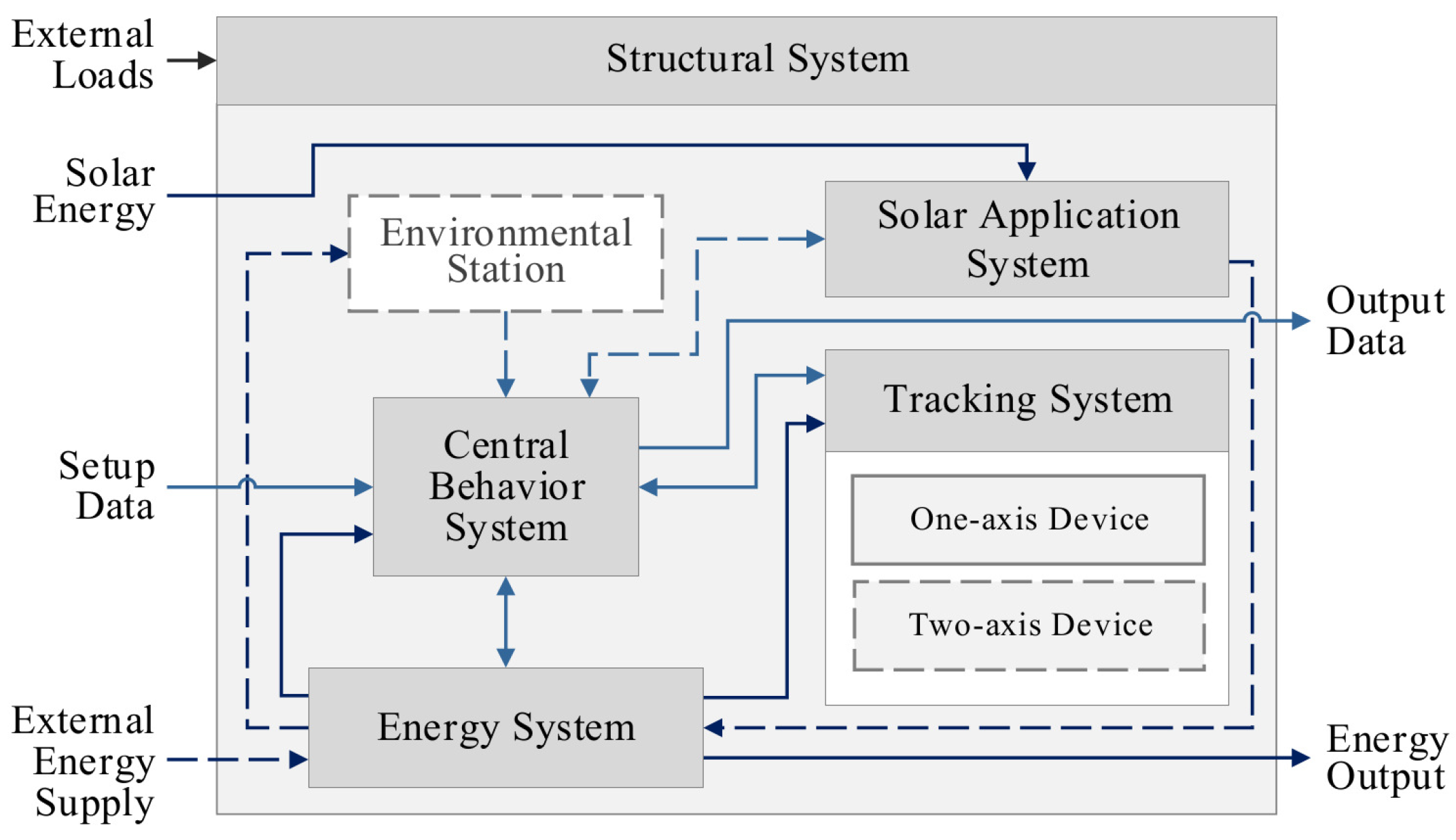
2. Physical Architecture of Solar Tracking Systems

Buede, in [34], defines the physical architecture of a system as the hierarchical description of the resources that comprise the system. Therefore, the physical architecture can be expressed as a model where the existing arrangement between the physical elements of the system is found, including the types of connection and the relation of inputs and outputs between the components. This facilitates the design process due to defines the required components, the system functions and their relationships to ensure the desired performance, by ensuring the design requirements. Therefore, a generic physical architecture is proposed for Solar Tracking Systems as shown in Figure 1.

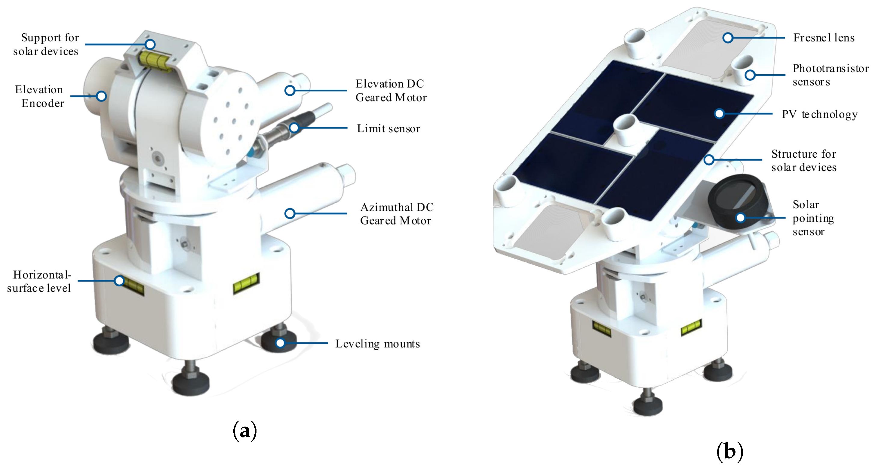
• Solar Application System. Is the solar technology that the solar tracker will use, the possible applications are Photovoltaic Systems (PVS), Concentrated Photovoltaic Systems (CPS), Thermal Systems (TS), Desalination Systems (DS), and special applications such as experimental platforms for calibration of solar sensors or measuring instruments. Each technology has special requirements, like the acceptance angle, which significantly affects the design process.
• Tracking System. It oversees following the solar path autonomously, fundamental purpose of the main system. Based on the number of axes required, a module can be defined for each one. The subsystem is integrated by an actuator, power transmission mechanisms, joint sensors, limit sensors, and electronic devices for actuators control.
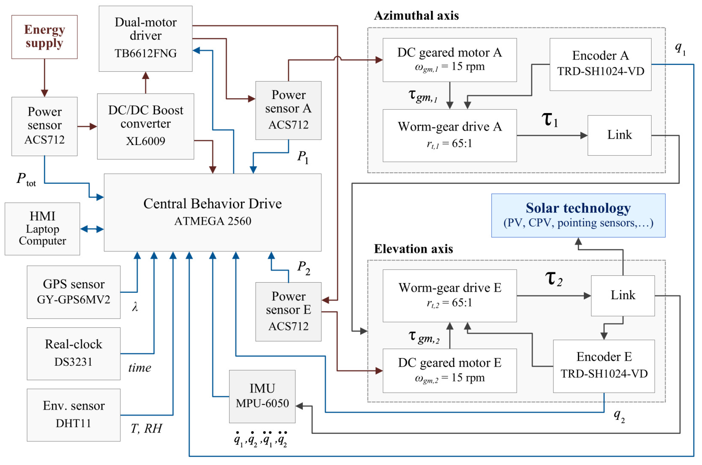
• Central Behavior System. It is responsible for the management of the behavior and energy strategies. It is integrated by the following components: Human–Machine Interface (HMI), programmable controllers, data loggers, and communication devices. The setup data include the selection of the operational mode, the tracker location, the day number, and the data required for the control of the system. The output data will depend on the tracker application and may include energy generation, energy consumption, tracking error, system status, and application data.
• Energy System. It includes the following components: power supply elements, power monitoring and converter devices, wiring devices, power protection devices, and, when applicable, power storage devices.
• Structural System. This system supports the internal and external loads, including the environmental conditions such as wind, temperature, rain, dust, among others.

Some STS have an Environmental Station that assists in the solar tracking process, as it measures the external parameters of the environment, allowing the system to make complex decisions. The station includes pyranometers, pyrheliometers, anemometers, wind vanes, temperature and humidity sensors, barometric pressure sensor, precipitation sensor, solar pointing sensor, solar irradiation sensor, among others.

The characteristics of STS can be classified as behavioral and physical, as shown in Figure 2. Both characteristics must be considered during the design process. The physical characteristics begin with the definition of the number of axes: one-axis or two-axis. Subsequently, it is required to define the STS configuration, for one-axis it can be vertical, horizontal, or tilted. For two-axis it can be tilt-roll or azimuth-elevation configuration. The behavioral characteristics begin with the selection of the tracking method. The open-loop method uses computational algorithms to determine the solar position, reducing the system complexity as additional devices are not required. The closed-loop method uses solar pointing sensors to define the real sun position, increasing the complexity of the system and requiring additional electrical energy for the sensing action. The mixed method alternates both tracking methods, implementing decision algorithms for the activation–deactivation action. Finally, the tracking strategy is defined. The step-by-step tracking strategy divides the solar trajectory into a finite number of points, holding the position for a time period. The continuous tracking strategy keeps the system moving in step with the solar movement.

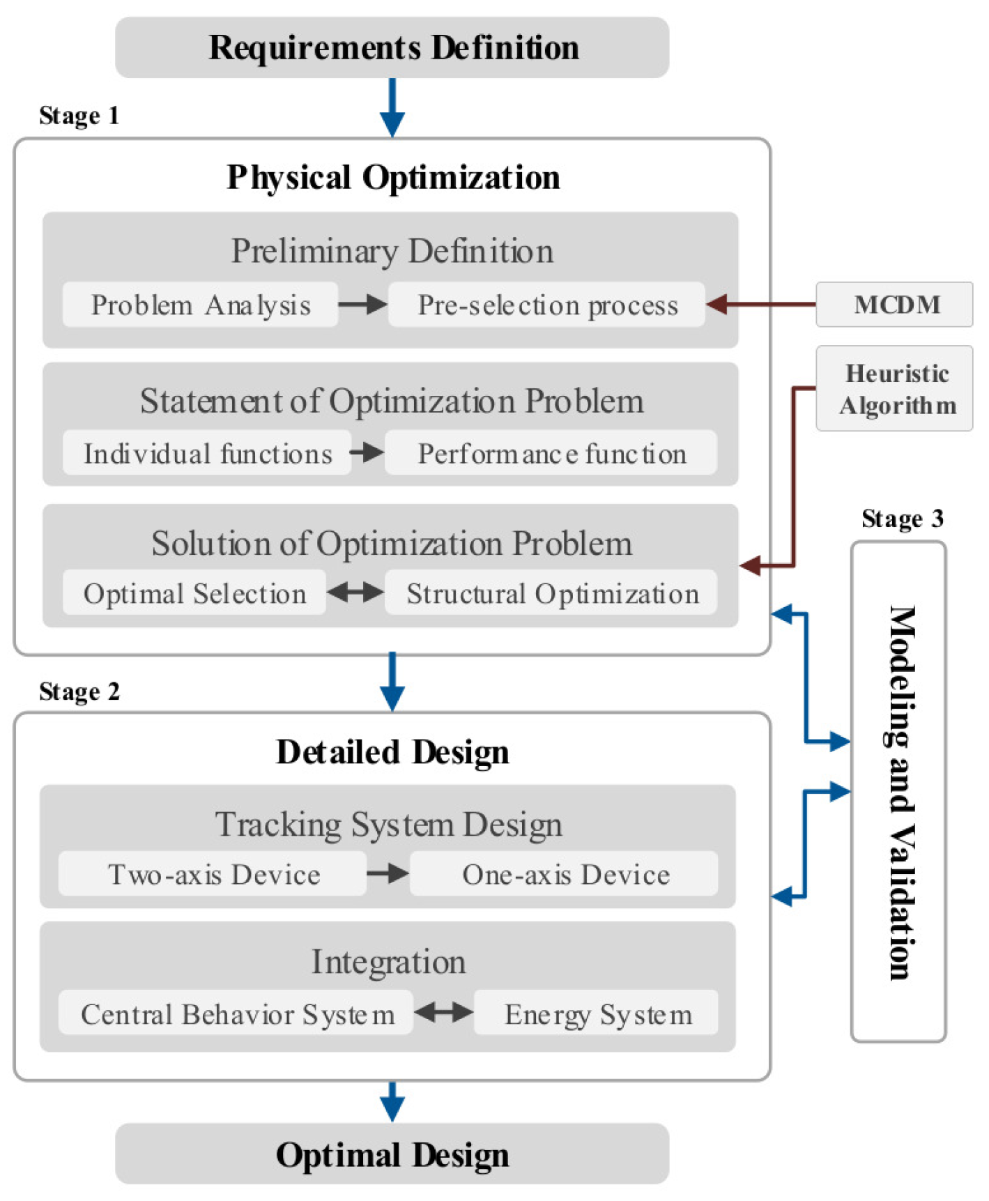
3. Problem Statement

The proposed strategy is presented for the optimal design of Solar Tracking Systems from a concurrent approach seeking the balance between the energy consumption and the tracking error. Commonly, this problem is solved independently, minimizing the tracking error or minimizing the energy consumption, affecting the general performance and the final energy balance of the STS. The methodology begins with the definition of the system requirements. Stafford specifies that each solar technology has specific requirements of tracking and relationships between the generated power and the tracking error [35]. Thus, the requirements must include at least the location of the STS, the ranges of the meteorological conditions, the solar application specifications, the behavior characteristics, and the physical characteristics (see Figure 2). According to the application, the models that will assist in the optimization process should be defined. For example, if the application is PV generation, a conversion efficiency model is required, including the solar insolation, the environmental temperature and the wind speed parameters. The strategy is divided into three stages as shown in Figure 3, two sequential stages and one parallel stage, each one is described below.

• Physical Optimization: The performance of the STS is affected by the performance of physical components, such as actuators and transmission elements, and by the geometric characteristics of the tracker. Optimal design is the selection of the physical components and the definition of the structural design, that minimize or maximize the performance function P. Therefore, the physical optimization can be defined as a Multi-objective Optimization Problem (MOP) [36], stated as follows:

  $$\mathrm{Minimize}P\left(\overline{x}\right)={[f_1\left(\overline{x}\right),f_2\left(\overline{x}\right),\dots ,f_n\left(\overline{x}\right)]}^T$$

  (1)

  subject to

  $$\begin{array}{c}\hfill g_i\left(\overline{x}\right)\le 0,i=1,2,\dots ,m\\ \hfill h_j\left(\overline{x}\right)=0,j=1,2,\dots ,r\end{array}$$

  where $P\left(\overline{x}\right)$ is the overall performance function, $f_i\left(\overline{x}\right)$ are the individual objective functions that represent the energy consumption and the tracking error, and $g_i\left(\overline{x}\right)$ and $h_j\left(\overline{x}\right)$ are the inequality constraints and equality constraints, respectively. The individual objective functions and the constraints expressions are any real valued function defined by the design parameters, and they can be piecewise, continuous, or non-continuous functions. The design vector is $\overline{x}=[{\overline{x}}_d,{\overline{x}}_s]$, $\overline{x}\in {\mathbb{R}}^n$, where ${\overline{x}}_d$ are continuous variables of the geometric characteristics and ${\overline{x}}_s$ are discrete variables of the parameters of the physical components. All the design variables must be bounded, sas they are related to the system implementation, representing real limitations such as sizes, tolerances, electrical power, among others. First, a pre-selection process is required to define a set of physical components that satisfy the system requirements, a MCDM must be used for the evaluation, being Multi-Attribute Utility Theory, Analytic Hierarchy Process, Fuzzy Set Theory, Goal Programming, Simple Additive Weighting, among others [37]. Second, the designer must define the individual objective functions according to the system requirements, that depict the overall system performance, establishing the overall performance function $P\left(\overline{x}\right)$. Finally, the optimization problem must be solved simultaneously, searching solutions for the optimal selection and for the optimal structural design.
• Detailed Design: It consists in the design of the axis devices, first with the second axis, and second with the first one. Once both modules are validated, the other systems must be detailed (see Figure 1). Finally, the integration process is carried out, it begins with the hardware integration and it ends with the software integration.
• Modeling and Validation: The modeling process consists of representing the STS from different approaches, at least the following models are required for the integral optimization: kinematic, dynamic, structural, tracking, and energy models, respectively. The validation is the process to determine if the suitable system has been developed [38], demonstrating that the STS fulfills the design purposes and the requirements in the desired environment. Commonly, the validations are supported by computational programs, obtaining numerical analysis and results. Some of the required validations are the following: energy balance, tracking error, structural analysis, and hardware–software validations.

4. Case Study

The proposed optimization strategy is implemented in a case study that consists of designing a STS for testing different solar technologies, such as a solar monitoring system. The system has the following characteristics: open-loop tracking method, step-by-step tracking strategy, two-axis, and azimuth-elevation configuration. As stage 3 is parallel, it will be developed in the stages 1 and 2.

4.1. Physical Optimization (Stage 1)

4.1.1. Preliminary Definition

Problem Analysis

For the definition of the torque in the elevation axis, a structural analysis is required. As the speed of the solar tracker is relatively low, the structural analysis can be considered as a static problem, and the torsional moments only affects the elevation axis. The external loads and the cross-sectional area of the elevation link are presented in Figure 4. The critical position is when the elevation angle $\alpha$ is equal to zero. Consequently, the total torque ${\tau }_2$ can be expressed as follows:

$${\tau }_2={\tau }_{c{m}_2}+{\tau }_{sc}+{\tau }_w$$

(2)

The torque caused by the center of mass of the link is ${\tau }_{c{m}_2}=l_{c{m}_2}·m_2·g$, and the mass of the link is expressed as $m_2=(a_2·b_2-a_1·b_1)·l_2·{\rho }_2$, where ${\rho }_2$ is the mass density, and $a_1$, $a_2$, $b_1$, $b_2$ are the geometric parameters of the cross-sectional area. The solar collector torque can be expressed as follows:

$${\tau }_{sc}=l_2·m_{sc}·g$$

(3)

where $m_{sc}$ is the mass of the solar collector, including the structural mass. Finally, the wind torque can be defined by

$${\tau }_w=0.00256·l_2·A_{sc}·C_d·v_w^2·sin{\beta }_w$$

(4)

where $A_{sc}$ is the area of the solar collector, $C_d$ is the drag coefficient, $v_w$ is the wind speed in mph, and the value $0.00256$ is a coefficient that involves the typical values for air density and gravitational acceleration in imperial units. Considering the power-train as shown in Figure 5, the geared motor torque ${\tau }_{gm}$, the gear ratio $r_t$, and the conversion efficiency ${\eta }_t$ of the transmission mechanism, the maximum torque in the elevation join can be expressed as follows:

$${\tau }_{max}={\tau }_{gm}·r_t·{\eta }_t$$

(5)

The total deformation of the elevation link can be defined through the method proposed in [39], composed by the deformation caused by the weight of the link ${\delta }_1$, by the solar collector ${\delta }_2$, and by the wind load ${\delta }_3$. They are expressed as follows:

$${\delta }_1=\frac{0.833·{\tau }_{c{m}_2}·l_2^2}{4·E·I},{\delta }_2=\frac{0.333·{\tau }_{sc}·l_2^2}{E·I},{\delta }_3=\frac{0.333·{\tau }_w·l_2^2}{E·I}$$

where E is the Modulus of Elasticity of the link, and I is the second moment of area. Therefore, the total deformation can be defined as

$${\delta }_T=\frac{l_2^2}{E·I}\left[0.208259·{\tau }_{c{m}_2}+0.333·({\tau }_{sc}+{\tau }_w)\right]$$

(6)

The maximum deformation ${\delta }_{max}$ depends on the acceptance angle ${\alpha }_a$ of the solar technology, being

$${\delta }_{max}=l_2·tan{\alpha }_a$$

(7)

The bending stress of the elevation link can be defined as

$${\sigma }_T=\frac{{\tau }_2·c}{I}$$

(8)

where c is the distance from the neutral axis to the external surface of the beam, equal to $c=b_2/2$. Finally, the maximum bending stress is proposed as follows:

$${\sigma }_{max}=\frac{{\sigma }_y}{3}$$

(9)

where ${\sigma }_y$ is the yield tensile strength of the link material.

Pre-Selection Process

The critical components of the system are the transmission mechanisms and the actuators of the axes. The Analytic Hierarchy Process, defined by Saaty in [40], is proposed to use as MCDM method. The scale for the evaluation was reduced from five to three levels, due to the complexity in the making decision process.

• Pre-selection of Transmission Components: The following types of transmissions were evaluated: Parallel shaft gears, planetary gears, harmonic-drive gears, worm gears, belt transmissions, and recirculating ball spindle. The data presented by Isermann in [41] are used for the definition of the criteria, being (1) Overall efficiency, (2) backlash, (3) self-locking device, (4) maintenance period, (5) maintenance difficulty, (6) additional components for reduce the backlash, (7) additional components for installation, (8) reduction ratio, (9) direct coupling, and (10) required space for installation. The expression (10) shows the values of the priority vector ${\overline{\omega }}_{tm}$. The worm-gears mechanism is the most suitable for the criteria, and a single-thread worm is recommended. The lead angle ${\lambda }_g$ in the worm-gears must be less than $5^{°}$ for self-locking condition.

  $${\overline{\omega }}_{tm}={\left[0.14800.17930.12040.03140.02340.18400.03460.15830.05750.0632\right]}^{⊺}$$

  (10)
• Pre-selection of Actuators: The possible actuators must have high conversion efficiency and low energy consumption. To increase the power transmission and to reduce the required power energy, actuators with gearboxes are considered in the selection process. The following types of electrical actuators were evaluated: DC excitation coil, DC permanent excitation, DC iron-less rotor, DC Brushless, and DC stepper motor. The data presented by Jung in [42] are used, being the following criteria: (1) power range, (2) rated voltage, (3) efficiency, and (4) control speed. The expression (11) shows the values of the priority vector ${\overline{\omega }}_{gm}$. The DC permanent excitation motor is that best meets the selection criteria.

  $${\overline{\omega }}_{gm}={\left[0.30450.06540.51430.1158\right]}^{⊺}$$

  (11)

In order to simplify the solution, a search for commercial components was carried out based on the problem analysis and the defined criteria.

Table 1. Parameters of standard pre-selected worm-gears transmission.

ID	Model	${\mathit{N}}_{\mathit{t}}$	${\mathit{r}}_{\mathit{t}}$	${\mathit{\eta }}_{\mathit{t}}$	${\mathit{\lambda }}_{\mathit{g}}{[}^{°}]$	${\mathit{m}}_{\mathit{t}}\left[\mathbf{kg}\right]$
${\mathrm{TM}}_1$	A 1B 6-N24018	18	18	0.82	4.77	0.0205
${\mathrm{TM}}_2$	A 1B 6-N32020A	20	20	0.80	4.08	0.0221
${\mathrm{TM}}_3$	A 1B 6-N32024	24	24	0.77	4.08	0.0253
${\mathrm{TM}}_4$	A 1B 6-N24030	30	30	0.75	4.77	0.0301
${\mathrm{TM}}_5$	A 1B 6-N24036	36	36	0.72	4.77	0.0376
${\mathrm{TM}}_6$	A 1B 6-N48040	40	40	0.71	3.58	0.0443
${\mathrm{TM}}_7$	S1B83A-C064B096D	48	48	0.68	3.583	0.0587
${\mathrm{TM}}_8$	S1B83A-C064B100D	50	50	0.67	3.583	0.0623
${\mathrm{TM}}_9$	S1B83A-C064B110D	55	55	0.65	3.583	0.0719
${\mathrm{TM}}_{10}$	S1B83A-C064B120D	60	60	0.63	3.583	0.0825
${\mathrm{TM}}_{11}$	S1B83A-C064B130D	65	65	0.61	3.583	0.0941
${\mathrm{TM}}_{12}$	S1B83A-C048B070S	70	70	0.59	3.583	0.0573
${\mathrm{TM}}_{13}$	S1B83A-C048B072S	72	72	0.58	3.583	0.0598
${\mathrm{TM}}_{14}$	S1B83A-C048B080S	80	80	0.55	3.583	0.0704
${\mathrm{TM}}_{15}$	S1B83A-C048B090S	90	90	0.50	3.583	0.0854

shows the pre-selected transmission components, where $N_t$ is the number of teeth of the worm-gear, $r_t$ is the gear ratio, ${\eta }_t$ is the estimated conversion efficiency, ${\lambda }_g$ is the lead angle, and $m_t$ is the mass. The model S1D96Z-P064SS of the worm is compatible for all the worm-gears, having the following parameters: AISI 303 stainless steel material, single thread, and mass of $0.0170$ kg.

Table 2. Parameters of pre-selected geared DC Motors.

ID	Model	${\mathit{\omega }}_{\mathit{gm}}$ [rpm]	${\mathit{P}}_{\mathit{e}}$ [W]	${\mathit{\tau }}_{\mathit{gm}}$ [Nm]
${\mathrm{GM}}_1$	1271-12-392	5	0.54	0.2
${\mathrm{GM}}_2$	1308-12-75	28	2.76	0.3
${\mathrm{GM}}_3$	1308-12-100	20	2.88	0.4
${\mathrm{GM}}_4$	3256-0	46	3.12	0.5
${\mathrm{GM}}_5$	BS138-4/12-608	5.3	0.90	0.5
${\mathrm{GM}}_6$	82862201	14	3.90	0.5
${\mathrm{GM}}_7$	82712006	35	1.44	0.5
${\mathrm{GM}}_8$	MR04A	15	0.96	0.6
${\mathrm{GM}}_9$	1308-12-200	10	3.00	0.8
${\mathrm{GM}}_{10}$	638178	30	6.00	0.9
${\mathrm{GM}}_{11}$	1308-12-250	8.5	2.88	1.0
${\mathrm{GM}}_{12}$	1308-12-510	5	1.80	1.0
${\mathrm{GM}}_{13}$	1308-12-630	4.5	1.56	1.0
${\mathrm{GM}}_{14}$	MR08B-012004	30	4.84	1.2
${\mathrm{GM}}_{15}$	638174	20	6.00	1.3
${\mathrm{GM}}_{16}$	PS-150-12-625	8.5	6.36	2.5
${\mathrm{GM}}_{17}$	E192-12-458	8.5	6.48	3.0
${\mathrm{GM}}_{18}$	E192-12-625	6	5.52	3.0
${\mathrm{GM}}_{19}$	114-41226-768	3.6	3.60	3.5
${\mathrm{GM}}_{20}$	638166	6	6.00	4.3

shows the pre-selected models geared DC motors, where $P_e$ is the electrical power, ${\omega }_{gm}$ is the rated speed, and ${\tau }_{gm}$ is the geared motor torque.

4.1.2. Statement of Optimization Problem

The aim of the problem statement is to find the best combination of the pre-selected components and the optimal design of the elevation link simultaneously. This optimization process only includes the Stage 1 of the proposed strategy. In accordance with the design objectives, the energy efficiency of the system can be related to the electrical power of the actuators. The tracking error can be associated to the total deformation of the elevation link, and to the worm-gears transmission efficiency. Therefore, the performance function can be composed by two individual objective functions, expressed as $P\left(\overline{x}\right)={[f_1\left(\overline{x}\right),f_2\left(\overline{x}\right)]}^T$, where the objective function $f_1\left(\overline{x}\right)$ depict the electrical power of the pre-selected elevation actuators, defined in Table 2, and the function $f_2\left(\overline{x}\right)$ depict the total deformation ${\delta }_T$ in the elevation link, as shown in expression (7). Therefore, the problem can be converted into a mono-objective problem by applying the Utility Function method presented in [36], and it can be stated as finding the optimal values of the design vector $\overline{x}$ such that

$$\mathrm{Minimize}P\left(\overline{x}\right)={\gamma }_1·f_1\left(\overline{x}\right)+{\gamma }_2·f_2\left(\overline{x}\right)$$

(12)

subject to

$$\begin{array}{c}\hfill g_1\left(\overline{x}\right)={\tau }_2-{\tau }_{max}\le 0\\ \hfill g_2\left(\overline{x}\right)={\delta }_T-{\delta }_{max}\le 0\\ \hfill g_3\left(\overline{x}\right)={\sigma }_T-{\sigma }_{max}\le 0\\ \hfill g_4\left(\overline{x}\right)=x_{d,3}-x_{d,1}\le 0\\ \hfill g_5\left(\overline{x}\right)=x_{d,4}-x_{d,2}\le 0\\ \hfill g_6\left(\overline{x}\right)=x_{d,1}-x_{d,2}\le 0\\ \hfill g_7\left(\overline{x}\right)=x_{d,3}-x_{d,4}\le 0\end{array}$$

where ${\gamma }_1=0.4$, and ${\gamma }_2=0.6$. The optimization problem is a Mixed Optimization Problem (MOP), due to the design vector $\overline{x}$ is composed by continuous and discrete variables, defined by $\overline{x}=\left[{\overline{x}}_d{\overline{x}}_s\right]$. The array of structural variables is composed by continuous variables and can be defined as ${\overline{x}}_d=\left[x_{d,1}{x}_{d,2}{x}_{d,3}{x}_{d,4}\right]=\left[a_2{b}_2{a}_1{b}_1\right]$ (see Figure 4). The array of the discrete variables is defined as ${\overline{x}}_s=\left[{\overline{x}}_{gm}{\overline{x}}_{tm}\right]$, where ${\overline{x}}_{gm}=\left[x_{gm,1}{x}_{gm,2}\right]=\left[{\tau }_{gm}{P}_e\right]$ are the geared motors parameters, and ${\overline{x}}_{tm}=\left[x_{tm,1}{x}_{tm,2}\right]=\left[r_t{\eta }_t\right]$ are the transmission components parameters.

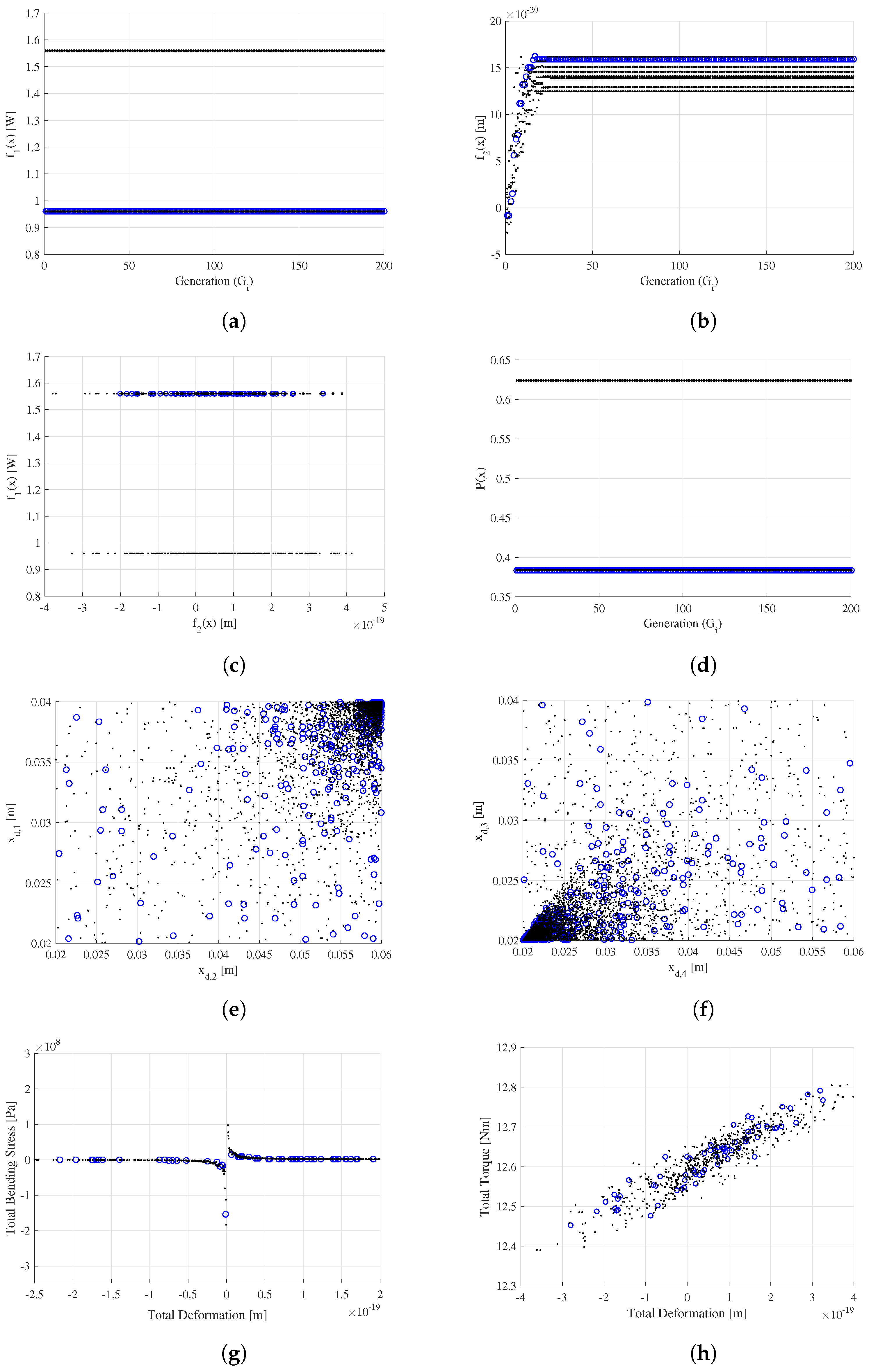
4.1.3. Solution of Optimization Problem

For the solution of the optimization problem, an heuristic algorithm is required: the general Differential Evolution (DE) method is proposed as a searching motor [43]; this heuristic technique can be used to solve complex engineering problems, which could be non-convex, discontinuous, or have discrete variables. It is the most accurate and robust algorithm of evolutionary strategies [44,45]. For the boundary constraint-handling, the rules proposed by Deb in [46] are used; these criteria allow selection of the solutions based on feasibility. The parameters required to solve the optimization problem using DE are the population size NP, the mutation factor F, and the crossover probability CR. For the solution of the Performance Function defined in (12), the algorithm shown in Figure 6 was proposed and implemented, where the maximum number of combinations is $\mathrm{Nc}=300$, and the number of convergence runs is $\mathrm{Nr}=30$. It was solved in the Mathworks Matlab^® R2020a software on a 64-bit computer, with Windows 7 operating system, Intel Core i7-4702HQ @2.20 GHz processor, and with 16 GB of RAM memory. The following parameters are considered: $l_2=0.075\mathrm{m}$, $g=9.81\mathrm{m}/{\mathrm{s}}^2$, $m_{sc}=30\mathrm{kg}$, $A_{sc}=0.994{\mathrm{m}}^2$, ${\beta }_w={45}^{°}$, $C_d=2.0$, $v_w=25\mathrm{km}/\mathrm{h}$, ${\rho }_2=2690\mathrm{kg}/{\mathrm{m}}^3$, ${\alpha }_{acc}={0.5}^{°}$, $E=68.9\times {10}^9\mathrm{Pa}$, ${\sigma }_y=89.6\times {10}^6\mathrm{Pa}$. For the DE algorithm, the population size per iteration was $\mathrm{NP}=20$, the maximum generations were $G_{max}=500$, used as a non-convergence criterion, the crossover factor was $\mathrm{CR}=0.65$, and the mutation factor was $F=0.7$. To ensure the convergence of the proposed algorithm, thirty runs were performed.

Table 3. Results of the individual objective functions and the Performance Function $P\left(\overline{x}\right)$ of the ten best combinations.

Rank	${\mathbf{C}}_{\mathit{i}}\left({\overline{\mathit{x}}}_{\mathit{s}}\right)$	${\mathbf{TM}}_{\mathit{p}}-{\mathbf{GM}}_{\mathit{q}}$	${\mathit{f}}_1\left(\overline{\mathit{x}}\right)$ [W]	${\mathit{f}}_2\left(\overline{\mathit{x}}\right)$ [m]	$\mathit{P}\left(\overline{\mathit{x}}\right)$
1	116	${\mathrm{TM}}_{11}-{\mathrm{GM}}_8$	0.96	$1.34\times {10}^{-19}$	0.384
2	117	${\mathrm{TM}}_{12}-{\mathrm{GM}}_8$	0.96	$7.05\times {10}^{-20}$	0.384
3	118	${\mathrm{TM}}_{13}-{\mathrm{GM}}_8$	0.96	$6.19\times {10}^{-20}$	0.384
4	119	${\mathrm{TM}}_{14}-{\mathrm{GM}}_8$	0.96	$1.01\times {10}^{-19}$	0.384
5	120	${\mathrm{TM}}_{15}-{\mathrm{GM}}_8$	0.96	$1.16\times {10}^{-19}$	0.384
6	185	${\mathrm{TM}}_5-{\mathrm{GM}}_{13}$	1.56	$2.20\times {10}^{-19}$	0.624
7	186	${\mathrm{TM}}_6-{\mathrm{GM}}_{13}$	1.56	$7.70\times {10}^{-20}$	0.624
8	187	${\mathrm{TM}}_7-{\mathrm{GM}}_{13}$	1.56	$8.34\times {10}^{-20}$	0.624
9	188	${\mathrm{TM}}_8-{\mathrm{GM}}_{13}$	1.56	$1.68\times {10}^{-20}$	0.624
10	189	${\mathrm{TM}}_9-{\mathrm{GM}}_{13}$	1.56	$2.48\times {10}^{-20}$	0.624

shows the results of the objective functions of the ten best combinations. The combinations that did not converge were discarded, being 142. The best combination is the number 116, composed by ${\mathrm{GM}}_8$ geared motor, and by the ${\mathrm{TM}}_{11}$ worm-gear transmission, the Performance function has a value of $0.384$. The convergence values of the objectives functions are $f_1\left(\overline{x}\right)=0.96$ W and $f_2\left(\overline{x}\right)=1.3452\times {10}^{-19}$ m. For the azimuthal module, the same combination was selected.

Table 4. Results of the design vector ${\overline{x}}_d$, ${\tau }_2$ [Nm], and ${\sigma }_T$ [MPa] of the ten best combinations.

Rank	${\mathit{C}}_{\mathit{i}}\left({\overline{\mathit{x}}}_{\mathit{s}}\right)$	${\mathit{\tau }}_{\mathit{max}}$ [Nm]	${\mathit{\sigma }}_{\mathit{T}}$ [MPa]	${\mathit{x}}_{\mathit{d},1}$ [m]	${\mathit{x}}_{\mathit{d},2}$ [m]	${\mathit{x}}_{\mathit{d},3}$ [m]	${\mathit{x}}_{\mathit{d},4}$ [m]
1	116	23.79	2.7338	0.0253	0.0494	0.0202	0.0297
2	117	24.78	4.5280	0.0391	0.0430	0.0322	0.0381
3	118	25.05	4.7088	0.0382	0.0392	0.0296	0.0338
4	119	26.40	3.5514	0.0391	0.0486	0.0333	0.0425
5	120	27.00	2.9715	0.0328	0.0464	0.0275	0.0340
6	185	25.92	1.8779	0.0266	0.0556	0.0249	0.0256
7	186	28.40	3.7828	0.0339	0.0392	0.0261	0.0283
8	187	32.64	3.7041	0.0317	0.0416	0.0253	0.0304
9	188	33.50	14.1287	0.0239	0.0321	0.0230	0.0274
10	189	35.75	10.4611	0.0344	0.0350	0.0264	0.0337

shows the values obtained of the design vector, as well as the maximum torque, and the total bending stress. Figure 7 shows the optimization results of the ten best combinations, the blue circles are the best value obtained from the 116 combination for each $G_i$ generation. Figure 7d shows the convergence of the performance function $P\left(\overline{x}\right)$; Figure 7a,b shows the individual functions convergence; and Figure 7e,f shows the solutions of the continuous variables $x_{d,1}$, $x_{d,2}$, $x_{d,3}$, and $x_{d,4}$. Figure 7g shows the total deformation versus the total bending stress, and Figure 7h shows the total deformation versus the total torque in the elevation link.

4.2. Detailed Design (Stage 2)

The criteria used for the selection of the remainder hardware were the fulfillment of the device functionality, energy consumption, and efficiency. The selected data processing device is an ATMega 2560, with 54 digital I/O ports, 16 analog I/O ports, 8 KB SRAM memory, 4 KB EEPROM memory, and 5 VDC operating voltage. For the measurement of the position of each axis, two incremental rotatory encoders were selected with the following characteristics: 1024 pulses per revolution, 5 VDC input voltage, up to 200 kHz response frequency, and 50 mA of mean current consumption. For the DC geared motors control, a dual-driver motor was selected; it has a standby system for energy save. For the energy conditioning, a DC-to-DC boost converter was selected, with a range of 7–35 V of output voltage, a maximum output current of $2.5$A, and $95\%$ of energy conversion efficiency. A real-time clock device was incorporated with a real-time, high-precision quartz watch; a backup battery that means the value of time is not lost; and an automatic compensation for leap-years and months. This device is very important for the open-loop solar tracking systems, due to the necessity of the astronomical algorithm to obtain the time clock as input to compute the solar vector. A relative humidity and temperature sensor was selected for the measurement of the environment conditions. Two optical limit sensors for setting the tracker home position are selected. To facilitate the process of installation and orientation of the tracker, an inclination device was incorporated which consist of a three-axis gyroscope and a three-axis accelerometer. The component is installed in the support of the solar devices mounting. This allows determining the initial angles of the tracker in the process of setup to determine the leveling of the system. Likewise, it serves to provide feedback to the tracker orientation, and to have a comparison with the values obtained by the encoders. The component has low energy consumption of approximately $0.008$ W. To automatically determine the location of the tracker, obtaining the geolocalization initial values for the calculation of the solar trajectory, a GPS satellite positioning module with data backup and low energy consumption was incorporated; its energy consumption is approximately $0.132$ W, the use of this module will be done only for the start-up of the tracker, and when it is relocated. Finally, three power sensors were selected, which determine in real-time the energy consumption of the tracker, which allows us to modify the tracking and energy saving strategies to reduce the overall energy consumption, based on the Hall effect, with accuracy of $\pm 1.5\%$. To validate the optimal design, the following simulations and computational analyses were carried out with favorable results: structural analysis, including deformation and stress analysis, assembly, and manufacturing processes simulation, tracking control simulation, alignments and interference between components, and simulation of the workspace of the tracker. The workspace for the azimuth movement is $0^{°}$ to ${360}^{°}$, and for the elevation movement $0^{°}$ to ${120.95}^{°}$. Figure 8 shows the detail design obtained by the proposed strategy; Figure 8a shows a 3D rendering model in isometric view of the tracker, including some selected components; and Figure 8b shows the STS with multiple solar devices mounted on the structural support. Figure 9 shows the interrelation between components of the obtained STS, including the power connections, data signals, and the physical connections.

5. Results and Discussion

According to the optimal design obtained by proposed strategy, the STS was manufactured and implemented, as shown in Figure 10.

5.1. Simulation and Experimental Results

For the simulation and experimental processes, the following was considered for the definition of the tracking error and energy analysis:

• The location was carried out at the Instituto de Energía Solar, Madrid, Spain, at the latitude ${40.4893}^{°}$ and longitude $-{3.6827}^{°}$. The day 20 June 2018, was considered, where the sunrise time was at 06:44:07, the sunset time was at 21:48:35, and the noon time was at 14:16:20, for a total of $15.8583$ h of sunlight. The experimental test began at 08:12:00 and ended at 19:53:00, with a total duration of 11.68 h as the solar pointing sensor is activated with a minimum of 300 W/m${}^2$.
• For the open-loop tracking method, the Solar Position Algorithm (SPA) was used [47]. The trajectory was segmented in 788 steps for azimuthal movement, and 434 for elevation movements. Based on the dynamic model of the STS presented in [33], a Generalized Proportional-Integral controller was developed [48]. This controller allows to obtain acceptable results with a low computational cost, which is reflected in savings of $26.98\%$ of energy consumption [33].
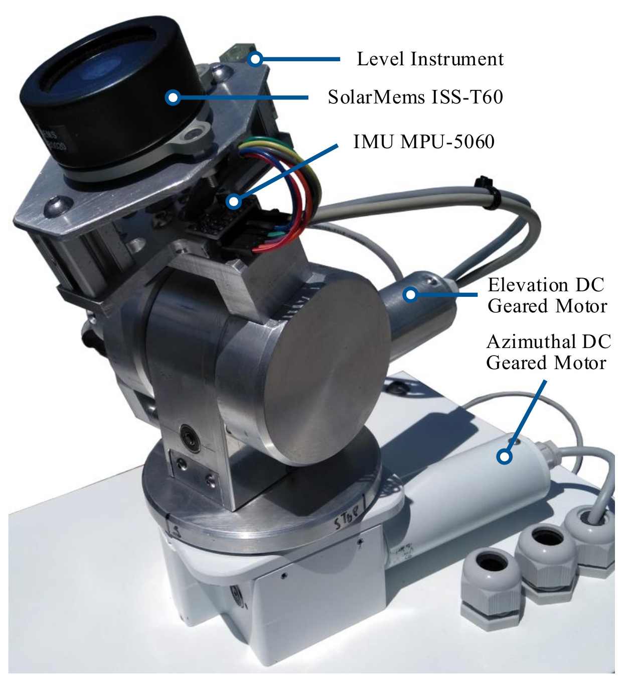
• A pointing sensor was used for the measurement of the experimental tracking error. The SolarMems^® sensor was connected to a laptop for the recording of the data. And, for the measurement of the energy consumption, three ACS712 power sensors were used at the measure points, as shown in Figure 9. These sensors were previously calibrated with a multimeter model Fluke 289 true RMS. The energy consumption was estimated by the following expression:

  $${\mathrm{EC}}_{\mathrm{tot}}\left(t\right)={\mathrm{EC}}_{\mathrm{axis}}+{\mathrm{EC}}_{\mathrm{H}}$$

  (13)

  where ${\mathrm{EC}}_{\mathrm{axis}}$ is the energy consumption of the axes, defined by

  $${\mathrm{EC}}_{\mathrm{axis}}={\mathrm{EC}}_{\mathrm{axis},1}+{\mathrm{EC}}_{\mathrm{axis},2}={\int }_0^{t_1}|P_1\left(\tau \right)|d\tau +{\int }_0^{t_2}\left|P_2\left(\tau \right)\right|d\tau$$

  (14)

  where $P_1\left(\tau \right)$ and $P_2\left(\tau \right)$ are the electrical power of the azimuthal and elevation axes, respectively. $t_1$ and $t_2$ are the time where the motors are active, considering that $t_1\ne t_2$, due to the trajectories and the number of steps for the tracking path are different for each axis. It is not necessary to consider the idle energy consumption at the holding position power because of the self-locking mechanisms. ${\mathrm{EC}}_{\mathrm{H}}$ is the energy required for the operation of the hardware devices such as sensors, motor drivers, electronic devices, etc.; it can be defined with the following expression:

  $${\mathrm{EC}}_{\mathrm{H}}={\mathrm{EC}}_{{\mathrm{h}}_{\mathrm{op}}}+{\mathrm{EC}}_{{\mathrm{h}}_{\mathrm{id}}}={\int }_0^{t_{op}}|P_h\left(\tau \right)|d\tau +{\int }_0^{t_{id}}\left|P_h\left(\tau \right)\right|d\tau$$

  (15)

  where $P_h\left(\tau \right)$ is the electrical power of the hardware devices, and $t_{op}$ and $t_{id}$ are the operation time and idle time, respectively. The idle time is defined as the period after tracking operation is completed, and the tracker is in a specific position waiting to move to the next position, the electronic devices are continued consuming energy for data processing, and for measuring and monitoring environmental parameters.

Figure 11 shows the bar graph of the comparison of the energy consumption between simulation and experimental test.

Table 5. Summarized simulation and experimental results of energy consumption.

Variable	Units	Simulation	Experimental
${\mathrm{EC}}_{\mathrm{axis}}$	Wh	$0.2282$	$0.1236$
${\mathrm{EC}}_{\mathrm{H}}$	Wh	$2.8376$	$2.6360$
${\mathrm{EC}}_{\mathrm{tot}}$	Wh	$3.0659$	$2.7597$

shows the mainly simulation and experimental results of the energy consumption, where the total energy consumption is $3.0659$ Wh for simulation and $2.7597$ Wh for experimental test. The simulation and experimental results of tracking errors are presented in

Table 6. Summarized simulation and experimental results of tracking error.

Variable	Units	Simulation	Experimental
${\epsilon }_{\theta }$	${}^{°}$	0.06	0.062
${\epsilon }_{\alpha }$	${}^{°}$	0.06	0.071
${\epsilon }_m$	${}^{°}$	$0.0849$	$0.0942$

, where the mixed error is ${0.0849}^{°}$ and ${0.0942}^{°}$ for simulation and experimental test, respectively.

5.2. Comparative Analysis

To determine if the obtained results by the proposed strategy are competitive, a comparison was made between four commercial systems with the same tracking application (solar monitoring system) and the developed tracker.

Table 7. Summarized parameters of commercial and developed STS.

Parameter	STS${}_1$	STS${}_2$	${\mathbf{STS}}_3$	${\mathbf{STS}}_4$	${\mathbf{STS}}_5$
Accuracy (Passive) [${}^{°}$]	<${0.1}^{°}$	<${0.1}^{°}$	-	-	<${0.09}^{°}$
Accuracy (Active) [${}^{°}$]	<${0.01}^{°}$	<${0.01}^{°}$	<${0.01}^{°}$	<${0.01}^{°}$	-
Angle resolution [${}^{°}$]	-	-	${0.009}^{°}$	${0.009}^{°}$	${0.0087}^{°}$
Gear-train	Worm-gear	Worm-gear	Harmonic	Harmonic	Worm-Gear
DC Motor type	Stepper	Stepper	Stepper	Stepper	Permanent
Torque [Nm]	35	12	12	24	24
Angular velocity [${}^{°}/s$]	$9.4$	$18.8$	-	-	$1.38$
Payload capacity [kg]	30	10	7	15	32
Power consumption [W]	<$3.92$	<$3.02$	<10	<10	<$2.75$
Elevation angle [deg]	-	-	$-{15}^{°}$ to ${95}^{°}$	$-{15}^{°}$ to ${95}^{°}$	$-{10}^{°}$ to ${110}^{°}$
Azimuthal angle [deg]	-	-	$0^{°}$ to ${360}^{°}$	$0^{°}$ to ${360}^{°}$	$0^{°}$ to ${360}^{°}$
Weight [kg]	25	8	$14.5$	$15.5$	$7.5$
Width [m]	$0.490$	$0.370$	$0.430$	$0.430$	$0.350$
Length [m]	$0.490$	$0.290$	$0.380$	$0.380$	$0.200$
Height [m]	$0.460$	$0.300$	$0.440$	$0.440$	$0.200$

shows the summarized parameters of the STS, where ${\mathrm{STS}}_1$ is the model SunTracker 3000 SMS and ${\mathrm{STS}}_2$ the model SunTracker 2000 SMS of the enterprise Hukseflux USA, ${\mathrm{STS}}_3$ is the model STR-21G and ${\mathrm{STS}}_4$ the model STR-22G of the enterprise EKO Instruments, and ${\mathrm{STS}}_5$ is the developed system. The pointing accuracy is similar to the ${\mathrm{STS}}_1$ and ${\mathrm{STS}}_2$ models because the tracking method is closed-loop. All four models employ a DC stepper motor type, which makes it difficult to reduce the tracking error due to its limited by the resolution of the steps in the motor, the tracker developed can further reduce the error by implementing another strategy of control, due to the DC permanent motor type. The ${\mathrm{STS}}_1$ model has the highest torque. However, the highest payload capacity has the developed tracker, due to the optimization in the process selection of the transmission components and actuators. The tracker has the lowest power consumption, $8.94\%$ less than the ${\mathrm{STS}}_2$, $29.84\%$ less than ${\mathrm{STS}}_1$, and $72.5\%$ less than the ${\mathrm{STS}}_3$ and ${\mathrm{STS}}_4$ models. According to weight, the developed system is the lightest, which improve the reduction of the energy consumption. Finally, the dimensions and the workspace of the five trackers are similar.

Although the application is not to generate electrical power, an energy analysis was carried out to validate the concurrent strategy. The yearly clear-sky insolation was made for Madrid, comparing between one-axis tracking and two-axis tracking (see Figure 12).

Table 8. Month and annual clear-sky insolation along with one and two-axis trackers.

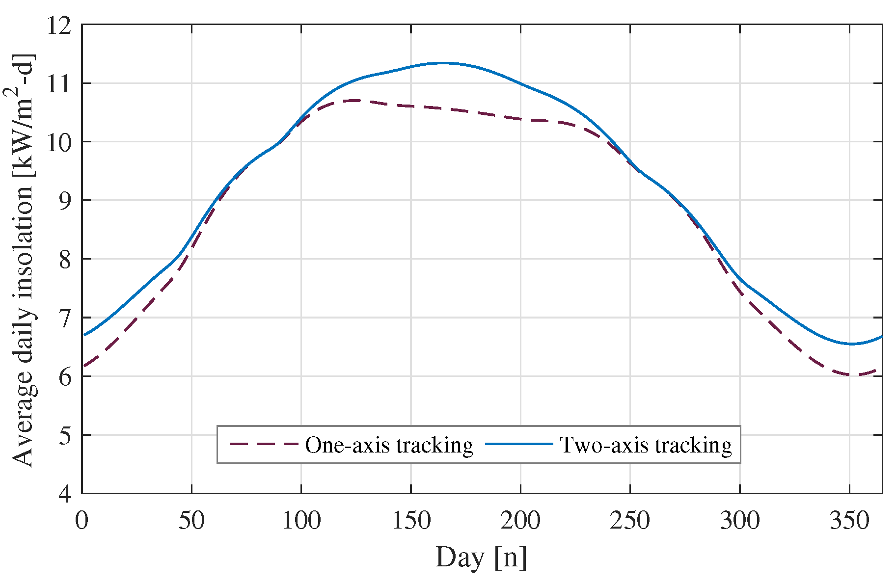
	Month Insolation [kW/m${}^2$-m]
Month	One-Axis	Two-Axis	${\%}_{\mathit{I}}$
Jan	206.4580	220.8760	$6.98\%$
Feb	222.7389	229.3483	$2.96\%$
Mar	294.8224	295.7353	$0.30\%$
Apr	313.3043	317.0220	$1.18\%$
May	330.3101	345.7804	$4.68\%$
Jun	316.5966	339.5153	$7.23\%$
July	322.6228	342.0917	$6.03\%$
Aug	315.9140	323.5156	$2.40\%$
Sept	281.5187	282.0640	$0.19\%$
Oct	250.1583	254.1680	$1.60\%$
Nov	201.8106	213.2003	$5.64\%$
Dec	188.6862	204.7313	$8.50\%$
Total [MW/m${}^2$-yr]	$3.2449$	$3.3680$	$3.7936\%$

shows the month and annual clear-sky, for the one-axis and two-axis configuration, which allows to observe that there is an increase in solar collection of $3.7936\%$ per year using the two-axis tracking, while in June it was approximately $7.23\%$. However,

Table 9. Hour-by-hour clear-sky insolation and environment temperature T${}_e$ in 20 June 2018, for Madrid, Spain.

	Insolation [W/m${}^2$]
Solar Time	One-Axis	Two-Axis	Te [°C]
07:00:00	75.1743	82.8279	17.7
08:00:00	497.0860	542.7491	18.9
09:00:00	706.3422	764.7833	21.5
10:00:00	816.1720	877.8104	24.6
11:00:00	877.0715	939.2781	26.3
12:00:00	909.4624	972.3091	27.7
13:00:00	924.1609	988.2975	29.3
14:00:00	928.0463	993.0215	30.7
15:00:00	924.1609	988.2975	32.0
16:00:00	909.4624	972.3091	32.7
17:00:00	877.0715	939.2781	33.1
18:00:00	816.1720	877.8104	32.0
19:00:00	706.3422	764.7833	31.4
20:00:00	497.0860	542.7491	32.5
21:00:00	75.17430	82.82795	31.8
Total [kW/m${}^2$-d]	$10.5389$	$11.3291$

and Figure 13 show the insolation comparison on the test day for both configurations, with an increase of $7.49\%$ using a two-axis tracker.

The power generation of photovoltaic technology also depends on parameters such as temperature [49,50,51], affecting the solar cells performance with an efficiency reduction between $2.9\%$ and $9.0\%$ [52]. Table 9 shows the environment temperature (T${}_e$) along the testing day, with a mean temperature of $28.62$ °C and maximum temperature of $33.1$ °C at 17:00 h. To ensure the least impact on the conversion efficiency of PV technology, it is recommended to keep the temperature as low as possible, even below $25$ °C [53], achieving maximum efficiency in PV panels on the temperature transition from $18$ °C to $25$ °C [50]. According to the authors of [49], there is no significant effect on the efficiency for temperatures between $25$ °C and $38$ °C, presenting a maximum reduction of $2.2\%$ in the power generated. Considering the models developed in [51], the largest efficiency loss at the highest temperature on the analyzed day would be $0.6804\%$ and $0.2673\%$ for the monocrystalline and polycrystalline panels, respectively. As the reduction in efficiency is low, and due to the fact that the comparison will be made under the same environmental conditions including the temperature changes along the day, the influence of the temperature parameter can be neglected in the comparative study carried out. To determine the real power available, it is recommended to use the Normal Operative Cell Temperature (NOCT), as it is a test standard adapted to the real operating conditions of photovoltaic cells [54]. However, it relates the reached temperature by open circuited cell to estimate the power. Consequently, to estimate the energy generated, the values of the efficiency obtained by the Standard Test Conditions (STC) of 1 kW/m${}^2$ insolation and temperature of $25$ °C defined by the producers were used [54]. Therefore, the energy generated can be estimated as follows:

$$\mathrm{EG}=\mathsf{\Delta }t·I·A_{pv}·{\eta }_{pv}$$

(16)

where I is the hourly insolation, $\mathsf{\Delta }t$ is the period with the insolation value, $A_{pv}$ is the area of photovoltaic array, and ${\eta }_{pv}$ is the conversion efficiency of the PV technology. According to the models presented in [55] and the tracking angles obtained from the SPA algorithm, the hour-by-hour clear-sky insolation was estimated (see Table 9).

Table 10. Parameters of commercial photovoltaic solar panels.

Model	${\mathit{A}}_{\mathit{pv}}$ [${\mathbf{m}}^2$]	${\mathit{m}}_{\mathit{pv}}\left[\mathbf{kg}\right]$	${\mathit{\eta }}_{\mathit{pv}}$	Type
${\mathrm{PV}}_1$	0.174	2.4	0.114	Monocrystalline
${\mathrm{PV}}_2$	0.157	3.0	0.158	Polycrystalline
${\mathrm{PV}}_3$	0.243	2.82	0.123	Monocrystalline
${\mathrm{PV}}_4$	0.240	3.1	0.124	Monocrystalline
${\mathrm{PV}}_5$	0.284	3.4	0.105	Polycrystalline
${\mathrm{PV}}_6$	0.340	4.5	0.146	Monocrystalline
${\mathrm{PV}}_7$	0.397	4.58	0.125	Monocrystalline
${\mathrm{PV}}_8$	0.515	6.74	0.155	Monocrystalline
${\mathrm{PV}}_9$	0.359	7.25	0.222	Monocrystalline
${\mathrm{PV}}_{10}$	0.697	7.26	0.143	Polycrystalline
${\mathrm{PV}}_{11}$	0.646	7.48	0.154	Monocrystalline
${\mathrm{PV}}_{12}$	0.665	9.0	0.150	Monocrystalline
${\mathrm{PV}}_{13}$	0.807	9.2	0.161	Monocrystalline
${\mathrm{PV}}_{14}$	0.994	12.0	0.150	Monocrystalline

shows the parameters of the commercial PV panels considered in the analysis. For the selection of the PV panels, the combination that could generate the largest amount of energy was determined based on the payload capacity of each of the trackers (see

Table 11. Summarized results of energy analysis and CO${}_2$ impact analysis.

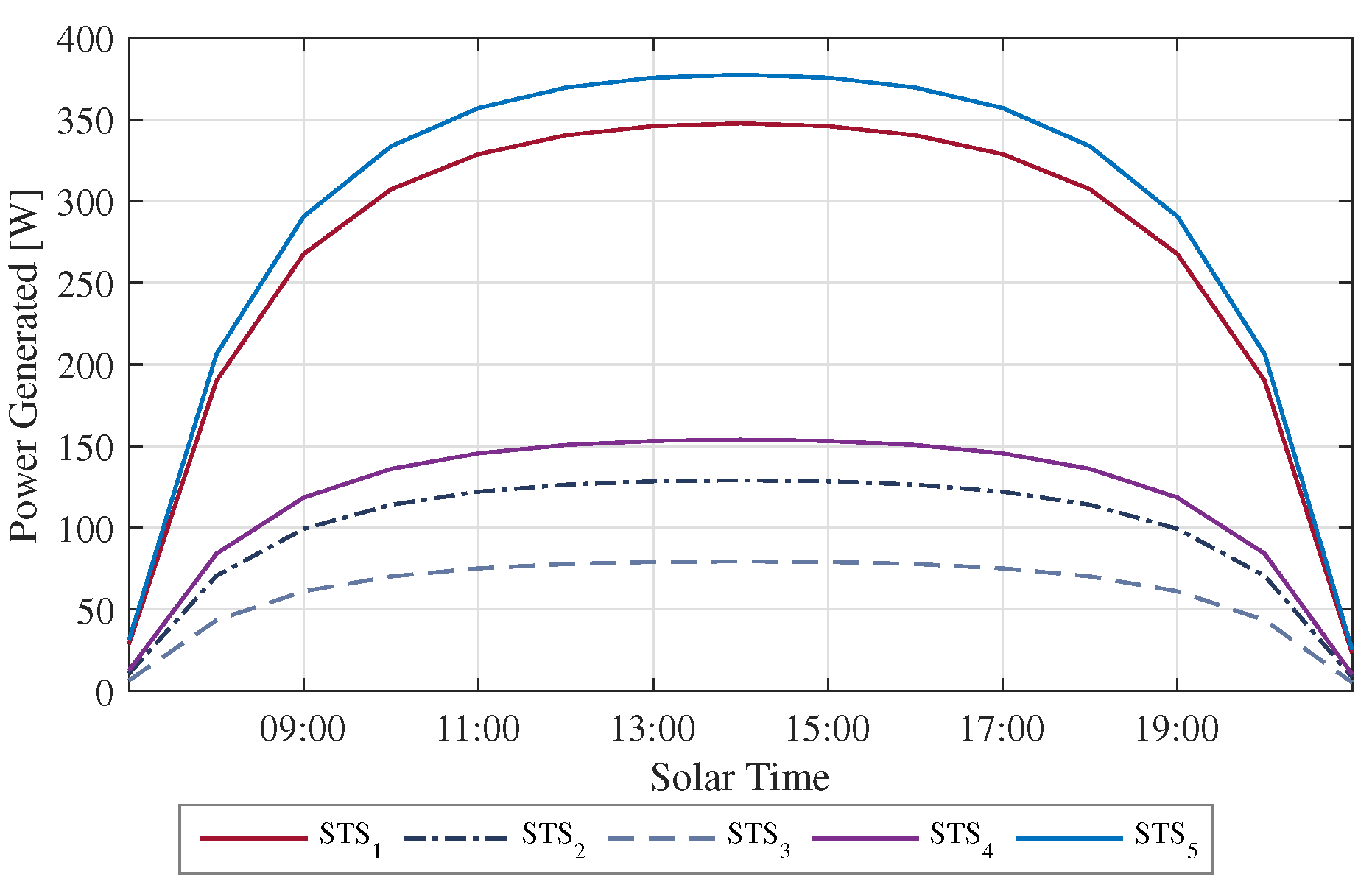
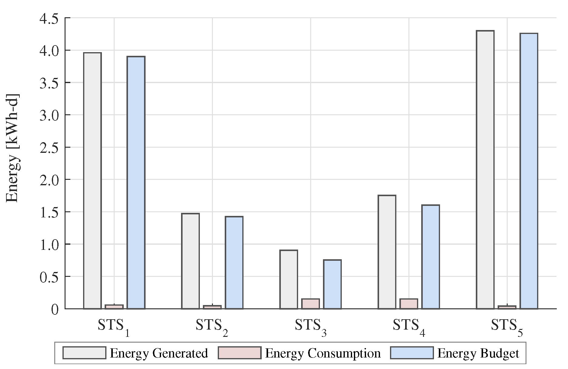
	Panels	${\mathbf{A}}_{\mathit{sc}}$	${\mathbf{m}}_{\mathit{sc}}$	EG	EC	EB	EC${}_{\%}$	CO${}_2$
STS	Array	[m${}^2$]	[kg]	[kWh-d]	[Wh-d]	[kWh-d]	$[\%]$	[g]
STS${}_1$	${\mathrm{PV}}_7-{\mathrm{PV}}_{14}-{\mathrm{PV}}_{14}$	2.3853	28.58	3.9600	59.0916	3.9009	1.4921	36.6368
STS${}_2$	${\mathrm{PV}}_{13}$	0.8074	9.20	1.4709	45.5246	1.4253	3.0950	28.2253
STS${}_3$	${\mathrm{PV}}_8$	0.5159	6.74	0.9053	150.7440	0.7546	16.6496	93.4612
STS${}_4$	${\mathrm{PV}}_2-{\mathrm{PV}}_{14}$	1.1515	15.00	1.7537	150.7440	1.6029	8.5955	93.4612
STS${}_5$	${\mathrm{PV}}_{10}-{\mathrm{PV}}_{14}-{\mathrm{PV}}_{14}$	2.6850	31.26	4.2998	41.4546	4.2583	0.9641	25.7018

).

Figure 14 shows the comparison of the estimated power generation in a clear day of the five solar trackers, where trackers STS${}_1$ and STS${}_5$ are the ones that generated the most electrical power. The energy budget can be expressed as the energy flow of the system, that is, system energy income minus energy expenditure. Figure 15 shows the comparison of the power budget of the trackers along the day.

Figure 16 shows the bar graph of the energy analysis of the systems. The developed system has the best energy budget, with $4.2583$ kWh-d, followed by the STS${}_1$ system, with $3.9009$ kWh-d. Considering that the tracking systems must use less than $3\%$ of the generated energy for the tracking action [56], the systems STS${}_1$, STS${}_2$, and STS${}_5$ are appropriate for solar power generation applications, where the developed system has the lowest percentage, with $0.9641\%$ as shown in Table 11.

It is important to determine the impact of CO${}_2$ from systems, due to the warming effect of CO${}_2$. The impact of CO${}_2$ is presented in Table 11, indicating the carbon impact for each solar tracker during the daytime operation, is obtained by multiplying the Energy Consumption of each tracker with the Greenhouse Gas (GhG) conversion rate of $0.41$ [gCO${}_2$/Wh], reported in CO${}_2$ emissions of electricity generation in Spain [57]. This factor depends on the country, is a function of the power generation technology mix in that country. The total estimated CO${}_2$ impact of the developed STS is $25.7018$ g, being the system with the lowest CO${}_2$ impact.

6. Conclusions and Future Work

This research proposes a novel concurrent strategy for the optimization of the global performance in STS at the design stage, allowing to select the optimal components of the system and to reduce the tracking error and the energy consumption in a balanced way. This strategy allows the definition of the objective functions depending on the tracking application, as well as the optimal selection of the critical components, and the optimal design of the system, simultaneously. The values obtained from the simulations are close to the experimental values, validating the system design previously the implementation, reducing cost of experimentation. To demonstrate the impact of the present proposal, the developed system was compared with four commercial systems. The pointing accuracy is competitive in open-loop method, being ${0.09}^{°}$. It is possible to achieve a similar accuracy to the other systems in a closed-loop by implementing a solar pointing sensor and an adequate control strategy. The developed tracker presents the best results in terms of energy consumption and energy budget, with a consumption percentage of $0.9641\%$, lower than the established by Mousazadeh in [56], which indicates that the tracking systems must have a consumption between 2–3% of the generated energy to be efficient. In comparison with other approaches, the strategy developed considerably improves energy consumption. In [58], a $5.6295\%$ percentage of energy consumed percentage is obtained with $21.215$ Wh for tracking action and $376.85$ Wh of generated energy, increasing approximately $26.9\%$ compared to a fixed system. Other developments may have lower values of energy consumption, such as in [59] with $0.08\%$. However, tracking accuracy is low, with high tracking errors around of $2^{°}$. This strategy finds a harmonic balance between energy consumption and tracking accuracy. Currently, the impact of CO${}_2$ is highly relevant in new technological developments, there are various analyzes in tracking systems [60,61,62], where it is established that two-axis systems are those that have the least impact. In the developed system, due to the high energy budget, the CO${}_2$ impact is reduced, and it is $8.94\%$ less than the commercial solar tracker with the lowest value. For Concentrated Photovoltaic Systems, where the STS are critical for the rise of the generation efficiency, the present strategy can improve the energy budget for this technology due to the design of tracking systems with low energy consumption and high tracking accuracy. Finally, as the application of the STS developed is for the measurement of solar parameters with sensor devices, the estimates and values obtained from the performance function in the design process are not affected by the temperature parameter, neither the results obtained from the experimental tests. However, for future research when using the proposed method to develop STS for power generation applying PV technology, the temperature parameter should be considered in the models, as it will significantly affect the conversion efficiency of photovoltaic technology.

References

- REN21. Renewables 2020 Global Status Report; Technical Report; REN21: Paris, France, 2020. [Google Scholar]
- Sofia, S.E.; Wang, H.; Bruno, A.; Cruz-Campa, J.L.; Buonassisi, T.; Peters, I.M. Roadmap for cost-effective, commercially-viable perovskite silicon tandems for the current and future PV market. Sustain. Energy Fuels 2020, 4, 852–862. [Google Scholar] [CrossRef] [Green Version]
- Stolterfoht, M.; Grischek, M.; Caprioglio, P.; Wolff, C.M.; Gutierrez-Partida, E.; Peña-Camargo, F.; Rothhardt, D.; Zhang, S.; Raoufi, M.; Wolansky, J.; et al. How to quantify the efficiency potential of neat perovskite films: Perovskite semiconductors with an implied efficiency exceeding 28%. Adv. Mater. 2020, 32, 2000080. [Google Scholar] [CrossRef] [PubMed]
- Jiang, X.; Zang, Z.; Zhou, Y.; Li, H.; Wei, Q.; Ning, Z. Tin Halide Perovskite Solar Cells: An Emerging Thin-Film Photovoltaic Technology. Acc. Mater. Res. 2021, 2, 210–219. [Google Scholar] [CrossRef]
- Hasan, A.; Dincer, I. A new performance assessment methodology of bifacial photovoltaic solar panels for offshore applications. Energy Convers. Manag. 2020, 220, 112972. [Google Scholar] [CrossRef]
- Muehleisen, W.; Loeschnig, J.; Feichtner, M.; Burgers, A.; Bende, E.; Zamini, S.; Yerasimou, Y.; Kosel, J.; Hirschl, C.; Georghiou, G. Energy yield measurement of an elevated PV system on a white flat roof and a performance comparison of monofacial and bifacial modules. Renew. Energy 2021, 170, 613–619. [Google Scholar] [CrossRef]
- Mohammadnia, A.; Ziapour, B.M. Investigation effect of a spectral beam splitter on performance of a hybrid CPV/Stirling/TEG solar power system. Appl. Therm. Eng. 2020, 180, 115799. [Google Scholar] [CrossRef]
- Valera, Á.; Rodrigo, P.M.; Almonacid, F.; Fernández, E.F. Efficiency improvement of passively cooled micro-scale hybrid CPV-TEG systems at ultra-high concentration levels. Energy Convers. Manag. 2021, 244, 114521. [Google Scholar] [CrossRef]
- Albert, P.; Jaouad, A.; Hamon, G.; Volatier, M.; Valdivia, C.E.; Deshayes, Y.; Hinzer, K.; Béchou, L.; Aimez, V.; Darnon, M. Miniaturization of InGaP/InGaAs/Ge solar cells for micro-concentrator photovoltaics. Prog. Photovolt. Res. Appl. 2021, 29, 990–999. [Google Scholar] [CrossRef]
- Jost, N.; Vallerotto, G.; Tripoli, A.; L’Eprevier, B.D.; Domínguez, C.; Askins, S.; Antón, I. Molded glass arrays for micro-CPV applications with very good performance. In AIP Conference Proceedings; AIP Publishing LLC: College Park, PA, USA, 2020; Volume 2298, p. 050003. [Google Scholar]
- Maliani, O.; Bekkaoui, A.; Baali, E.; Guissi, K.; El Fellah, Y.; Errais, R. Investigation on novel design of solar still coupled with two axis solar tracking system. Appl. Therm. Eng. 2020, 172, 115144. [Google Scholar] [CrossRef]
- Meng, X.l.; Liu, C.l.; Bai, X.h.; Kong, D.h.; Du, K. Improvement of the performance of parabolic trough solar concentrator using freeform optics and CPV/T design. AIMS Energy 2021, 9, 286–304. [Google Scholar] [CrossRef]
- Vallerotto, G.; Victoria, M.; Jost, N.; Askins, S.; Domínguez, C.; Herrero, R.; Antón, I. Comparison of achromatic doublet on glass Fresnel lenses for concentrator photovoltaics. Opt. Express 2021, 29, 20601–20616. [Google Scholar] [CrossRef]
- Wang, G.; Wang, F.; Shen, F.; Jiang, T.; Chen, Z.; Hu, P. Experimental and optical performances of a solar CPV device using a linear Fresnel reflector concentrator. Renew. Energy 2020, 146, 2351–2361. [Google Scholar] [CrossRef]
- Barbón, A.; Bayón-Cueli, C.; Bayón, L.; Ayuso, P.F. Influence of solar tracking error on the performance of a small-scale linear Fresnel reflector. Renew. Energy 2020, 162, 43–54. [Google Scholar] [CrossRef]
- Du, X.; Li, Y.; Wang, P.; Ma, Z.; Li, D.; Wu, C. Design and optimization of solar tracker with u-pru-pus parallel mechanism. Mech. Mach. Theory 2021, 155, 104107. [Google Scholar] [CrossRef]
- Morón, C.; Ferrández, D.; Saiz, P.; Vega, G.; Díaz, J.P. New prototype of photovoltaic solar tracker based on arduino. Energies 2017, 10, 1298. [Google Scholar] [CrossRef]
- Alexandru, C. Optimizing the mechanical device of a mono-axial sun tracking mechanism. In MATEC Web of Conferences; EDP Sciences: Les Ulis, France, 2018; Volume 184, p. 01001. [Google Scholar]
- Lim, B.H.; Lim, C.S.; Li, H.; Hu, X.L.; Chong, K.K.; Zong, J.L.; Kang, K.; Tan, W.C. Industrial design and implementation of a large-scale dual-axis sun tracker with a vertical-axis-rotating-platform and multiple-row-elevation structures. Sol. Energy 2020, 199, 596–616. [Google Scholar] [CrossRef]
- Jamroen, C.; Komkum, P.; Kohsri, S.; Himananto, W.; Panupintu, S.; Unkat, S. A low-cost dual-axis solar tracking system based on digital logic design: Design and implementation. Sustain. Energy Technol. Assess. 2020, 37, 100618. [Google Scholar] [CrossRef]
- Zhu, Y.; Liu, J.; Yang, X. Design and performance analysis of a solar tracking system with a novel single-axis tracking structure to maximize energy collection. Appl. Energy 2020, 264, 114647. [Google Scholar] [CrossRef]
- Quesada, G.; Guillon, L.; Rousse, D.R.; Mehrtash, M.; Dutil, Y.; Paradis, P.L. Tracking strategy for photovoltaic solar systems in high latitudes. Energy Convers. Manag. 2015, 103, 147–156. [Google Scholar] [CrossRef]
- Alexandru, C. Optimal design of the dual-axis tracking system used for a PV string platform. J. Renew. Sustain. Energy 2019, 11, 043501. [Google Scholar] [CrossRef]
- Marcu, A.; Alexandru, C.; Barbu, I. Dynamic optimization of a dual-axis solar tracker for PV modules. In IOP Conference Series: Materials Science and Engineering; IOP Publishing: Bristol, UK, 2019; Volume 514, p. 012037. [Google Scholar]
- Gutierrez, S.; Rodrigo, P.M.; Alvarez, J.; Acero, A.; Montoya, A. Development and Testing of a Single-Axis Photovoltaic Sun Tracker through the Internet of Things. Energies 2020, 13, 2547. [Google Scholar] [CrossRef]
- Fuentes-Morales, R.F.; Diaz-Ponce, A.; Peña-Cruz, M.I.; Rodrigo, P.M.; Valentín-Coronado, L.M.; Martell-Chavez, F.; Pineda-Arellano, C.A. Control algorithms applied to active solar tracking systems: A review. Sol. Energy 2020, 212, 203–219. [Google Scholar] [CrossRef]
- Fernández-Ahumada, L.; Ramírez-Faz, J.; López-Luque, R.; Varo-Martínez, M.; Moreno-García, I.; de la Torre, F.C. Influence of the design variables of photovoltaic plants with two-axis solar tracking on the optimization of the tracking and backtracking trajectory. Sol. Energy 2020, 208, 89–100. [Google Scholar] [CrossRef]
- Mi, Z.; Chen, J.; Chen, N.; Bai, Y.; Fu, R.; Liu, H. Open-loop solar tracking strategy for high concentrating photovoltaic systems using variable tracking frequency. Energy Convers. Manag. 2016, 117, 142–149. [Google Scholar] [CrossRef]
- Sallaberry, F.; Pujol-Nadal, R.; Larcher, M.; Rittmann-Frank, M.H. Direct tracking error characterization on a single-axis solar tracker. Energy Convers. Manag. 2015, 105, 1281–1290. [Google Scholar] [CrossRef]
- Flores-Hernández, D.; Palomino-Resendiz, S.; Lozada-Castillo, N.; Luviano-Juárez, A.; Chairez, I. Mechatronic design and implementation of a two axes sun tracking photovoltaic system driven by a robotic sensor. Mechatronics 2017, 47, 148–159. [Google Scholar] [CrossRef]
- Shams, M.H.; Kia, M.; Heidari, A.; Zhang, D. Optimal design of photovoltaic solar systems considering shading effect and hourly radiation using a modified PSO algorithm. Simulation 2019, 95, 931–939. [Google Scholar] [CrossRef]
- Aste, N.; Del Pero, C.; Leonforte, F.; Manfren, M. A simplified model for the estimation of energy production of PV systems. Energy 2013, 59, 503–512. [Google Scholar] [CrossRef]
- Flores-Hernandez, D.A.; Palomino-Resendiz, S.I.; Luviano-Juárez, A.; Lozada-Castillo, N.; Gutierrez-Frias, O. A heuristic approach for tracking error and energy consumption minimization in solar tracking systems. IEEE Access 2019, 7, 52755–52768. [Google Scholar] [CrossRef]
- Buede, D.M.; Miller, W.D. The Engineering Design of Systems: Models and Methods; John Wiley & Sons: Hoboken, NJ, USA, 2016. [Google Scholar]
- Stafford, B.; Davis, M.; Chambers, J.; Martínez, M.; Sanchez, D. Tracker accuracy: Field experience, analysis, and correlation with meteorological conditions. In Proceedings of the 2009 34th IEEE Photovoltaic Specialists Conference (PVSC), Philadelphia, PA, USA, 7–12 June 2009; pp. 002256–002259. [Google Scholar]
- Rao, S.S. Engineering Optimization: Theory and Practice; John Wiley & Sons: New Delhi, India, 2019. [Google Scholar]
- Velasquez, M.; Hester, P.T. An analysis of multi-criteria decision making methods. Int. J. Oper. Res. 2013, 10, 56–66. [Google Scholar]
- Hirshorn, S.; Voss, L.; Bromley, L. NASA Systems Engineering Handbook; NASA Technical Reports Server: Washington, DC, USA, 2017.
- McKenzie, W.M. Examples in Structural Analysis; CRC Press: Boca Raton, FL, USA, 2006. [Google Scholar]
- Saaty, T.L. Decision making with the analytic hierarchy process. Int. J. Serv. Sci. 2008, 1, 83–98. [Google Scholar] [CrossRef] [Green Version]
- Isermann, R. Mechatronic Systems: Fundamentals; Springer Science & Business Media: Berlin/Heidelberg, Germany, 2007. [Google Scholar]
- Jung, R.; Schneider, J. Elektische Kleinmotoren. Konstruktions-katalog und Marktübersicht. Feinw. Meßtechnik 1984, 92, 153–165. [Google Scholar]
- Storn, R.; Price, K. Differential evolution–a simple and efficient heuristic for global optimization over continuous spaces. J. Glob. Optim. 1997, 11, 341–359. [Google Scholar] [CrossRef]
- Villarreal-Cervantes, M.G.; Rodríguez-Molina, A.; García-Mendoza, C.V.; Peñaloza-Mejía, O.; Sepúlveda-Cervantes, G. Multi-Objective On-Line Optimization Approach for the DC Motor Controller Tuning Using Differential Evolution. IEEE Access 2017, 5, 20393–20407. [Google Scholar] [CrossRef]
- Civicioglu, P.; Besdok, E. A conceptual comparison of the Cuckoo-search, particle swarm optimization, differential evolution and artificial bee colony algorithms. Artif. Intell. Rev. 2013, 39, 315–346. [Google Scholar] [CrossRef]
- Deb, K. An efficient constraint handling method for genetic algorithms. Comput. Methods Appl. Mech. Eng. 2000, 186, 311–338. [Google Scholar] [CrossRef]
- Reda, I.; Andreas, A. Solar position algorithm for solar radiation applications. Sol. Energy 2004, 76, 577–589. [Google Scholar] [CrossRef]
- Sira-Ramírez, H. Sliding Modes, Δ-Modulators, and Generalized Proportional Integral Control of Linear Systems. Asian J. Control 2003, 5, 467–475. [Google Scholar] [CrossRef]
- Zaini, N.; Ab Kadir, M.; Izadi, M.; Ahmad, N.; Radzi, M.; Azis, N. The effect of temperature on a mono-crystalline solar PV panel. In Proceedings of the 2015 IEEE Conference on Energy Conversion (CENCON), Johor Bahru, Malaysia, 19–20 October 2015; pp. 249–253. [Google Scholar]
- Machniewicz, A.; Knera, D.; Heim, D. Effect of transition temperature on efficiency of PV/PCM panels. Energy Procedia 2015, 78, 1684–1689. [Google Scholar] [CrossRef] [Green Version]
- Elibol, E.; Özmen, Ö.T.; Tutkun, N.; Köysal, O. Outdoor performance analysis of different PV panel types. Renew. Sustain. Energy Rev. 2017, 67, 651–661. [Google Scholar] [CrossRef]
- Du, Y.; Fell, C.J.; Duck, B.; Chen, D.; Liffman, K.; Zhang, Y.; Gu, M.; Zhu, Y. Evaluation of photovoltaic panel temperature in realistic scenarios. Energy Convers. Manag. 2016, 108, 60–67. [Google Scholar] [CrossRef]
- Skoplaki, E.; Palyvos, J.A. On the temperature dependence of photovoltaic module electrical performance: A review of efficiency/power correlations. Sol. Energy 2009, 83, 614–624. [Google Scholar] [CrossRef]
- Lazaroiu, G.C.; Longo, M.; Roscia, M.; Pagano, M. Comparative analysis of fixed and sun tracking low power PV systems considering energy consumption. Energy Convers. Manag. 2015, 92, 143–148. [Google Scholar] [CrossRef]
- Gilbert, M.M. Renewable and Efficient Electric Power Systems; John Wiley & Sons: Hoboken, NJ, USA, 2004. [Google Scholar]
- Mousazadeh, H.; Keyhani, A.; Javadi, A.; Mobli, H.; Abrinia, K.; Sharifi, A. A review of principle and sun-tracking methods for maximizing solar systems output. Renew. Sustain. Energy Rev. 2009, 13, 1800–1818. [Google Scholar] [CrossRef]
- REE. CO2 Emissions of Electricity Generation in Spain; Technical Report; Red Eléctrica de España: Madrid, Spain, 2021. [Google Scholar]
- Sidek, M.; Azis, N.; Hasan, W.; Ab Kadir, M.; Shafie, S.; Radzi, M. Automated positioning dual-axis solar tracking system with precision elevation and azimuth angle control. Energy 2017, 124, 160–170. [Google Scholar] [CrossRef]
- Abdollahpour, M.; Golzarian, M.R.; Rohani, A.; Zarchi, H.A. Development of a machine vision dual-axis solar tracking system. Sol. Energy 2018, 169, 136–143. [Google Scholar] [CrossRef]
- Konneh, K.V.; Masrur, H.; Othman, M.L.; Wahab, N.I.A.; Hizam, H.; Islam, S.Z.; Crossley, P.; Senjyu, T. Optimal Design and Performance Analysis of a Hybrid Off-Grid Renewable Power System Considering Different Component Scheduling, PV Modules, and Solar Tracking Systems. IEEE Access 2021, 9, 64393–64413. [Google Scholar] [CrossRef]
- Sneineh, A.A.; Salah, W.A. Design and implementation of an automatically aligned solar tracking system. Int. J. Power Electron. Drive Syst. 2019, 10, 2055. [Google Scholar] [CrossRef]
- Prinsloo, G.; Dobson, R.; Schreve, K. Carbon footprint optimization as PLC control strategy in solar power system automation. Energy Procedia 2014, 49, 2180–2190. [Google Scholar] [CrossRef] [Green Version]