
Uncertainty in Unit Commitment in Power Systems: A Review of Models, Methods, and Applications


1
Department of Electrical Engineering, Chung Yuan Christian University, Taoyuan 32023, Taiwan
2
Electrical Engineering Department, Technological Institute of the Philippines, Manila 1001, Philippines
*
Author to whom correspondence should be addressed.
Energies 2021, 14(20), 6658; https://doi.org/10.3390/en14206658
Submission received: 31 August 2021
/
Revised: 23 September 2021
/
Accepted: 11 October 2021
/
Published: 14 October 2021
(This article belongs to the Section F: Electrical Engineering)
Abstract
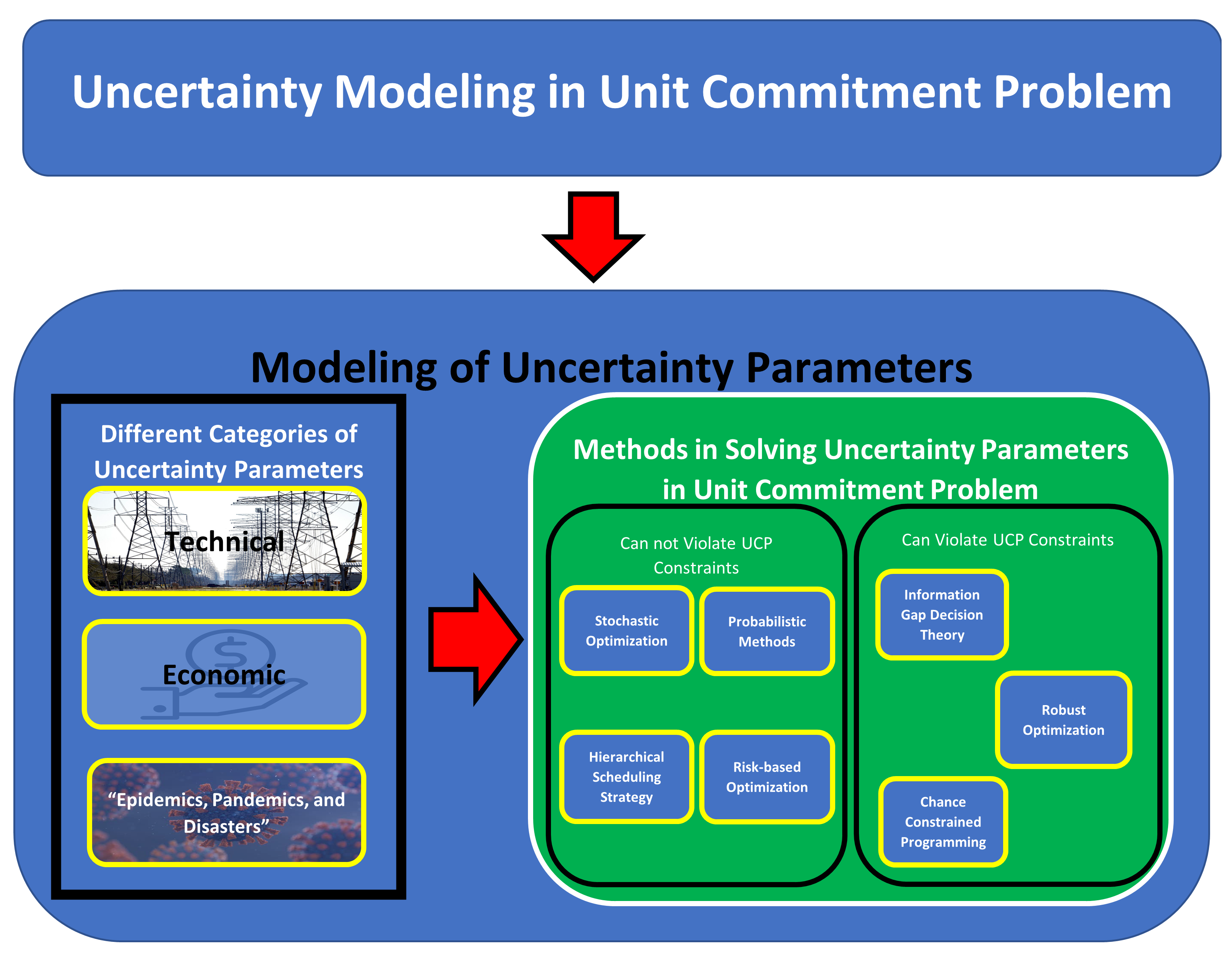
:The unit commitment problem (UCP) is one of the key and fundamental concerns in the operation, monitoring, and control of power systems. Uncertainty management in a UCP has been of great interest to both operators and researchers. The uncertainties that are considered in a UCP can be classified as technical (outages, forecast errors, and plugin electric vehicle (PEV) penetration), economic (electricity prices), and “epidemics, pandemics, and disasters” (techno-socio-economic). Various methods have been developed to model the uncertainties of these parameters, such as stochastic programming, probabilistic methods, chance-constrained programming (CCP), robust optimization, risk-based optimization, the hierarchical scheduling strategy, and information gap decision theory. This paper reviews methods of uncertainty management, parameter modeling, simulation tools, and test systems.

1. Introduction
A UCP involves the optimization of the ON/OFF states of generation units by minimizing the total operational cost while considering different constraints, in a particular period, generally one day/week. This problem arises mainly from the changing nature of human activities, which result in frequent load changes in each interval (minute, hour, day). Changes in load patterns require a change in available generation power plants. Mathematically, this problem is to optimize a set of completely mixed and nonlinear integer equations under different constraints to minimize the operational cost by solving the optimal combination of units from all possible scenarios.
In the last century, the UCP has continued to be significant, on account of developments and other changes in the power industry. Environmental policies, restructuring, privatization of the grid, penetration of RE, and the advent of smart grids have resulted in many changes and randomness in the power grid.
Uncertainties associated with various input parameters in the grid have raised several operational issues for system operators and other stakeholders. According to Ebeed et al. [1], the uncertainties of the parameters can be classified into two general categories: — uncertainties of technical parameters and those of economic parameters. The COVID – 19 pandemic has resulted in an unexpected global economic and social dilemma [2], leading to the identification of a third category of “epidemics, pandemics, and disasters”, all of which have techno-socio-economic effects on the energy sector.
Uncertainty affects schedules and may raise new challenges for the power grid. Various techniques and methods have been studied and employed to control the consequences of uncertainties associated with parameters.
Different studies and reviews were published considering uncertainty management. Uncertainty management can be implemented using different decision – making techniques [3] and various system optimization algorithms [4,5,6,7]. Abujarad et al. [5] discussed different optimization approaches for a UCP considering intermittent renewable energy resources. Dai et al. [6] provided a summary of different SP applications in a UCP. Lastly, Jurković et al. [7] highlighted the advantages and disadvantages of commonly used methods (stochastic, robust, and interval) in UCPs for uncertainty management. Unlike previous studies, this paper will focus on a review of previously implemented methods such as stochastic programming, probabilistic methods, CCP, RO, risk-based optimization, hierarchical scheduling strategy, and IGDT in uncertainty management considering technical, economical, and “epidemics, pandemics, and disasters” parameters.
The objectives of this paper are as follows:
- Delve into research that has considered uncertainty in the unit commitment problem.
- Discuss models, methods, test systems, and simulation tools that are used for uncertainty management.
- General comparison of different methods in terms of hardware specification, solver, run – time, and results.
This paper is structured as follows: Section 2 formulates the general unit commitment problem. Section 3 shows the modeling of different uncertainties that are considered in relation to unit commitment. Section 4 briefly reviews methods or techniques that are used to address these uncertainties. Section 5 addresses the different constraints that are applied in each method as well as the implemented test systems and simulation tools. Section 6 presents general notes on reviewed methods or techniques in addressing uncertainties. Lastly, Section 7 concludes by presenting the most important findings.
2. Unit Commitment Formulation
A UCP is a high-dimensional, mixed-variable, and complex problem because of its combinatorial behavior. The UCP involves the minimization of cost or maximization of profit. The formulation in this section involves all commonly used cost functions and constraints from various studies. Section 5 will summarize them.
2.1. Objective Function
The general expression of the objective function in the UCP is minimizing the total cost of running all the units for a given time. The difference between TC and TR is defined as,
where TC, or total operation cost, is specified mainly in terms of fuel cost, shutdown, start-up, emissions, and social welfare cost. TR represents the total revenue because of market involvement. The essential parameter that affects TR is the payment method, which is specified in terms of market operations and market-clearing mechanisms. All of these must be optimized by taking into account the constraints that govern the problem. In the classical UCP, TR is not considered because the market is regulated.
2.2. Different Terms of Objective Function
Section 2.2 presents the terms associated with TC and TR.
2.2.1. Total Cost Terms
The five cost terms are fuel, start-up, shutdown, emission, and social welfare cost functions.
TC is calculated as,
The social welfare and emission functions are not directly included in the TC term and will be considered in a multi-objective optimization framework.
Fuel Cost Function
The fuel cost function of a thermal generator is given in quadratic form. The conventional form of this function is as follows.
Emission Function
Emission function is presented in a non-linear form as follows.
Social Welfare Function
Social welfare function involves the so-called penalty cost function. Social welfare is maximized when this penalty cost function is minimized. Table 1 shows the different models of this function and the studies that consider them.
Start-Up Cost
In a thermal power plant, the start-up cost varies on fuel and emission prices, along with depreciation costs. These costs vary on off-time and therefore on a generator’s temperature at the time when it is started up again. Mostly, a basic approach is implemented to specify the start – up cost. This cost is a function of the operational status of the thermal generator and can be allocated into cold and hot start – up costs, as follows.
The start – up cost of a thermal generator is modeled as,
Shutdown Cost
Most of the time, the shutdown cost is constant. This cost is developed as a constant term for each thermal generator, which is shut down in a specified hour.
2.2.2. Total Revenue of Generation Companies
The total revenue is taken from the sales of power. The three main approaches for payment are PPD, PRA, and PPRP. Abdi reviewed these methods [54].
2.3. Problem Constraints
This subsection presents the primary constraints in the UCP.
2.3.1. System Constraints
System constraints, known as global constraints, are important in the UCP. The main system constraints are as follows.
System Energy Balance or Real Power Constraints
Energy Constraints
Reserve Constraints
Transmission Losses
The transmission losses are considered as follows.
2.3.2. Unit Constraints (Local Constraints)
Unit constraints are the local constraints that are considered on each generating unit. They are as follows.
Power Unit Limits
Reserve Unit Limits
Unit Minimum Up/Down Times (MUT/MDT)
Ramp Rate Limits (RRLs)
Unit Status Limits
Several units may be needed to be online at a specified duration (must run) or may become offline due to scheduled maintenance or forced outages (must not run), due to reliability issues, economic factors, or operating limitations.
2.3.3. Security Constraints
In the SCUCP, security constraints are developed as follows.
AC Power Flow Constraints
Transmission Line MVA Flow Limits
Bus Voltage Constraints
3. Modeling of Uncertainty
The challenges that are raised by uncertain parameters in the power grid have encouraged operators to use different uncertainty modeling techniques to prepare for their consequences and to make the best decisions. Table 2 shows works concerning each category of uncertainty.
The uncertainties of parameters can be classified as technical, economic, and “epidemics, pandemics, and disasters”. The following subsection will describe each model of uncertain parameters in the power system.
3.1. Outage or Failure of Any Element (Lines, Generators, or Others)
3.2. Load Demand Uncertainty Model
3.3. Wind Energy Uncertainty Model
Wind speed is an important parameter in determining wind energy output. The distribution of wind speeds can be modeled as a Weibull PDF or as Rayleigh PDF. Equations (22) and (23) describe the Weibull PDF and Rayleigh PDF of wind speed [23], respectively.
A Weibull PDF with is called a Rayleigh PDF.
The output wind power can be expressed by means of various models. Table 4 presents commonly used models.
3.4. PV Energy Uncertainty Model
The PV energy output is affected by the irradiance at the location. The probability distribution of irradiance is represented as a lognormal PDF as follows [127,128,129].
The probability distribution of solar irradiance can also be expressed using the Beta distribution function as follows.
where and are parameters in the beta probability function. The parameter of the Beta PDF can be assessed using the standard deviation and mean of the random variable [128,129]:
The output PV power can be expressed using different models. Table 5 presents commonly used models.
3.5. PEVs Uncertainty Model
3.6. Load Growth Uncertainty Model
Load growth is essential information in the research of a power system; it is also considered to be a random parameter. denotes the initial load in the base year while is the incremental load growth in year y. Therefore, the load in year y is . Its PDF can be expressed as follows [122]:
3.7. Electricity Price Uncertainty Model
3.8. Epidemics, Pandemics, and Disasters
Natural disasters such as typhoons, droughts, tsunamis, and earthquakes may generate uncertainty in the power grid. No base model exists for this category as each type of disaster can have certain consequences in the system (it can cause outages of power system components, a deficiency of supply, or excess supply). Huang et al. modeled the spillage of water from hydropower plants as an uncertain parameter [100]. Arab et al. proposed a post-disaster model that considered whether a component was “damaged” or “functional” [116]. Components that are classified as “damaged” undergo repairs for a specified time, and the VOLL is included in the UCP. Zhao et al. considered the worst load forecasting and line failure scenario in the UCP after a hurricane has occurred [36]. Pandemics and epidemics are presently highly significant,—specifically due to the COVID-19 pandemic [2]. This category will motivate new studies and modeling techniques since it influences the energy sector not only techno-economically but socially as well.
4. Different Methods Used for Uncertainty in Unit Commitment
The previous section considered the models of different uncertain parameters in the power grid. Different methods are required to solve the UCP with these uncertain parameters. Ebeed et al. [1] and Majidi et al. [133] classified these methods as possibilistic, probabilistic, hybrid possibilistic – probabilistic, IGDT, robust optimization, and interval analysis. This section discusses the methods considered in the literature review.
4.1. Stochastic Programming
SP is an approach that is risk-neutral and optimizes the expected outcome over a known probability distribution. Li et al. provided a brief history and review of stochastic programming methods [134]. They also discussed instances of SP, such as two – stage SP, multistage SP, multistage SP that goes through endogenous uncertainty, and scenario tree generation that is data-driven. Table 7 presents studies in which stochastic programming was used and the uncertain parameters modeled.
4.2. Probabilistic Methods
A PDF is identified for each random input parameter. Numerical and analytical methods are the commonly known category of probabilistic approaches or uncertainty modeling methods.
4.2.1. Numerical Methods
Numerical methods are mathematical tools used to find the uncertain input parameter. The main drawback of this method, also known as the conventional or purely mathematical method, is its high dimensionality and computing time. The following subsection will discuss MCS and MCMCS.
Monte Carlo Simulation
The MCS is applied to develop the probabilities of several outcomes of a process that cannot easily be predicted owing to the involvement of random variables. This is used to understand the impact of uncertainty and risk in forecasting and prediction models. Table 8 lists studies in which the MCS method was used and the uncertain parameters that were modeled in them. Most studies that use this method focus on renewable energy and demand as sources of uncertainty for the power grid.
Markov Chain MCS
MCMCS is a dynamic variation of the MCS method that is utilized to manage the uncertainty of parameters of a system. In this method, MCMCS is used to generate the samples based on the probability distribution, in which the probability of creating a unique state in the chain is based only on the present state.
In the MCMCS implementation, the probability of change is defined using the Metropolis method, which states that transition probability from state to , is while the probability of the accepted state is [1].
Table 9 presents studies in which the MCMS method has been used and the uncertain parameters that are modeled in them.
4.2.2. Analytic Methods
Different analytical methods (scenario – based and PDF approximation) are established for calculation with PDFs of uncertain input parameters.
Scenario-Based Method
The scenario – based method is a simple and efficient method for developing probabilistic uncertainties in which the continuous space of an uncertain function is converted into discrete scenarios with subsequent probabilities, and the PDF curve is divided into subregions [1]. Each region denotes a scenario that has a particular probability. Suppose that the divided regions have k = 1,2, 3…, N and their subsequent probabilities are , , , …, . The expected output value is given by,
The scenario-based method approximates and provides the expected values of the output functions.
Table 10 lists studies in which a scenario – based method is used, and the associated uncertain parameters. Scenario Trees are most used in the scenario-based method. Other methods include the WILMAR model, the PEM, GP regression, and the Roulette Wheel.
PDF Approximation
Approximate methods provide a simple description of the uncertain parameters by random variables. The main advantage of these methods is the use of deterministic routines for solving the UCP. In addition, approximate methods are computationally more efficient than other probabilistic methods.
Table 11 presents studies in which the PDF approximation method was used, the uncertain parameters modeled, and the type of technique considered. This method has been mostly applied to uncertainties with demand and renewable energy.
4.3. Chance Constrained Programming
The core idea of conventional CCP is to permit constraint violation. The probability violation must be smaller than a predefined risk level (confidence interval). A general form of a chance constraint is as follows. [40]
The symbol “Pr{•}” indicates the value of a probability.
CCP is regarded as solving a stochastic problem with some probabilistic constraints, such that certain constraints that are related to some uncertain parameters are fulfilled with a given probability.
Table 12 presents different studies in which CCP is used and the uncertain parameters modeled. A significant number of studies uses CCP to deal with uncertainties that are generated by wind power and demand.
4.4. Robust Optimization
RO methods are commonly used for uncertainty management in power systems. For instance, RO methods are used to solve the optimization problem with the worst scenario concerning the uncertain parameters.
Table 13 lists studies in which robust optimization is used and how this method is implemented for uncertain parameters. Different studies consider the uncertainty set to have fixed limits [15,16,17,18,22], while others model it as a flexible one [25,27,31]. MCS [17,94], PSO [82], and historical data [15,22,29,114,115] are commonly used to generate the uncertainty set for the reviewed studies.
4.5. Risk-Based Optimization
Risk-based optimization is based on the definition of risk measures and associated optimization problem formulation that accounts for the risk induced in system-level outputs by uncertain parameters.
Table 14 presents studies in which risk-based optimization is used, and the risk considered. Risk-based optimization is performed by adding a penalty term in the objective function [10,98], or by including the risk to constraints in the UCP [28,84], or by doing both [39,49,50,77]. Additional constraints are defined in [77,84] while others integrate the risk in the energy balance [98] and reserve constraint [28,49,50]. Wind power [10,28,39,49,98], demand [10,50,84], and failure of units [28,49,77] are considered as uncertain parameters in the risk-based optimization.
4.6. Hierarchical Scheduling Strategy
A hierarchical scheduling strategy is the process of scheduling components or entities according to rank of importance. In a UCP, it can be carried out concerning committed generation units or reserve allocation [23,24], [88].
Table 15 presents studies in which the hierarchical scheduling strategy is used and how this method is implemented for uncertain parameters modeling. Power trading is implemented in [23] to manage the uncertainty of renewable energy and demand. In this study, the penalty cost of power trading between microgrids is implemented through the hierarchical approach considering the least cost. In [24], the author emphasize that the tie-line schedule is solved first before considering the generation schedule when a power interchange occurs during load uncertainty. Lastly, in [88], the study implements a hierarchical scheduling strategy considering generation reserve, ramping reserve, and transmission reserve. This method is implemented in the UCP using the energy balance constraint and penalty cost function.
4.7. Information Gap Decision Theory (IGDT)
IGDT identifies the extent to which an uncertain parameter can function while ensuring that the minimum income is received by the decision – maker. Its two essential features are robustness and opportuneness. A detailed review of this approach can be found in the paper by Majidi et al. [133].
Table 16 presents the studies in which the IGDT method is used and how this method is implemented for uncertain parameters. The studies discussed in Table 16 consider a robust function wherein the uncertainty level is maximum when the function is maximized. The IGDT may be applied to the UCP by adding a penalty cost to the objective function; the IGDT’s robust function is integrated into the energy balance constraint.
4.8. Discussion of Reviewed Methods
A comprehensive review of the different studies and the method implementation were discussed in Section 4.4, Section 4.5, Section 4.6 and Section 4.7. These include SP, probabilistic methods, CCP, RO, risk-based optimization, hierarchical scheduling strategy, and IGDT. SP is a method that optimizes the expected outcome on a risk-neutral perspective using a probability distribution. Commonly used PDFs are Gaussian, Rayleigh, Weibull, and Beta Distribution. In most cases, this method is transformed into a deterministic approach making it much simpler and easily implemented. Renewable energy and demand uncertainty are the most common areas of study that implement this method. The PDF can be formulated using historical data, forecasted data, or simulation results. Aside from using a given PDF, other ways of generating input are numerical and analytic methods which fall under the second discussed method which is the probabilistic method. This method together with SP has been applied by many studies involving outages, demand, and renewable uncertainty. Unfortunately, using these two methods may lead to an infeasible solution due to the constraint violation. In this case, the use of IGDT and CCP methods can be applied. These two methods can relax constraint violations by augmenting a penalty factor when these violations are relaxed.
CCP is an approach wherein a constraint violation is allowed. When these constraints are violated, a penalty cost is introduced on the UCP. Commonly used penalty costs are related to the load shedding and wind spillage of renewable energy spillage. Like the SP and probabilistic methods, the expected outcome can be compared over a known PDF or interval. Unfortunately, CCP does not consider the given interval or known PDF, resulting in a limitation of its flexibility and robustness. IGDT, on the other hand, like the CCP, allows constraint violations. The difference is that a robust function is implemented in IGDT. In this method, the framework is independent of the PDF or membership set and it allows the SO to vary the operating strategy easily.
The risk-based method, unlike the SP, optimizes the UCP using a risk-level approach. Most of the studies that applied this method involve the wind power and demand uncertainty. Unlike the SP, the reserve allocation in the UCP is fixed and cannot be adjusted; the risk-based optimization allows violations on constraints at a given risk level. Some risk-based methods consider the penalty cost while others just integrate it in the energy balance constraint or in the reserve constraint.
The other two methods discussed in Section 4 are the hierarchical scheduling strategy and RO. The hierarchical scheduling strategy is, unlike SP, CCP, and IGDT, a hierarchical process which is implemented to mitigate the effect of uncertainty. Reserve allocation is the common application of this method. RO solves the UCP by considering the worst-case scenario which may not be considered by the previous methods.
Lastly, since more uncertainty parameters in the UCP can be considered, it results in more data and variables to be considered. Different methods may be integrated together to increase computational efficiency.
5. Evaluation of Constraints, Test System, and Simulation Tools of Different Studies
Table 17 gives an outline of studies on the UCP that consider uncertainty. The constraints that are applied in the problem, along with the test system and the applied simulation tools, are shown in each scenario.
A variety of constraints are identified in the studies and the demand balance and constraints on thermal units are mentioned in most of them.
The studied systems range from simple systems to IEEE bus systems and sometimes real-life grids with periods of 4, 24, 168, and 8760 h. Most of the studies involve the IEEE test system for 24 h.
CPLEX and GUROBI have been the most used solvers to be implemented using C, C++, Python, MATLAB, and GAMS. In most of the studies, MATLAB and GAMS have been used for simulation owing to their availability and ease of use.
6. General Notes on Reviewed Methods
Section 6 discusses some important issues regarding the reviewed methods. Table 18 summarizes all the reviewed studies in this paper in terms of method, solver, hardware specification, run – time, and simulation results. Based on Table 18, the following information can be summarized:
- As the system size increases, the corresponding run – time also increases.
- As more constraints are included in the UCP, the solution steps require a longer run time.
- The modeling of uncertainty parameters affects the UCP result.
- The CPLEX solver can be applied to any method.
- The Gurobi solver is used on some methods where uncertainty can be adjusted; they include CCP, risk-based optimization and RO.
- Advanced computing tools result in short run time regardless of methods applied.
- SP has been used in the majority of the studies due to the short run – time. The drawback is it may result in a sub-optimal result or infeasible solution due to its limitation. SP combined with other methods will optimize the solution but increase the run time. This has been the commonly used strategy due to the advancement of computing tools.
- RO has become of interest to a lot of researchers since it can handle more constraints compared to other methods. The only drawback to this method is its run – time, but this has already been solved due to more advanced computing tools.
7. Conclusions
Uncertainty management in a UCP is crucial in the operations, control, and monitoring of power systems. It has attracted considerable attention since it influences the cost of the operation and maintenance of power grids. Considering the significance of this topic, this paper reviews a significant number of studies in this area.
The review identifies various types of uncertainty parameters and identifies how each is modeled. These types are technical, economic, and “epidemics, pandemics, and disasters”. The latter category is found to be of great importance because this type cannot be modeled as simply as the first two types because it affects not only the techno-economic aspect of the energy sector but also the social aspect and thus, may lead to future studies.
This review examines various methods for uncertainty management and describes key concepts and innovations. The management of uncertainties related to renewable energy has seen an increase in studies conducted in recent years. These uncertainties arise from sustainable grid reconstruction and evolving environmental policies. In addition, the management of uncertainties related to electricity prices and demand continue to be of great importance today. These uncertainties arise from market liberalization and the increase in world population.
Computing tools such as GAMS and MATLAB are identified as the most used software tools, along with CPLEX or GUROBI solvers. For the studied system, IEEE test systems using 24-h intervals are easily implemented owing to data availability and their ease of use. A realistic test system (real power grid) should also be considered in conducting the uncertainty management of a UCP. Robust optimization has recently become a method of interest due to the availability of highly advanced computing tools. Lastly, this review shows how different studies propose policies or strategies in improving the control and operation for power systems. These strategies include the hierarchical scheduling of reserve, penalty cost for RE spillage and load shedding, and proper management of thermal units and ESS.
Author Contributions
Conceptualization, Y.-Y.H.; methodology, G.F.D.A.; writing—original draft preparation, G.F.D.A.; supervision, Y.-Y.H.; funding acquisition, Y.-Y.H. All authors have read and agreed to the published version of the manuscript.
Funding
This research was funded by the Ministry of Science and Technology in Taiwan, grant number MOST 110-3116-F-008-001.
Institutional Review Board Statement
Not applicable.
Informed Consent Statement
Not applicable.
Data Availability Statement
Not applicable.
Acknowledgments
The authors would also like to thank the editors and reviewers for their valuable insight and suggestions on this paper.
Conflicts of Interest
The authors declare no conflict of interest.
Abbreviations
| ACPF | AC Power Flow |
| ADP | Adaptive Dynamic Programming |
| ATC | Analytical Target Cascading |
| BB | Branch/Bound |
| BCD | Block Coordinate Descent |
| BESS | Battery Energy Storage System |
| BPECI | Bulk Power Energy Curtailment Index |
| BPII | Bulk Power Interruption Index |
| BVC | Bus Voltage Constraint |
| CCP | Chance Constrained Programming |
| CCTS | Chance – Constrained Two – Stage |
| CHP | Combined Heat and Power |
| CFSDP | Clustering by Fast Search and the finding of Density Peaks |
| CVaR | Conditional Value-at-Risk |
| DDRC | Data-driven Distributionally Robust Chance – Constrained |
| DG | Distributed Generation |
| DHN | District Heating Network |
| DLOL | Duration of Loss of Load |
| DR | Demand Response |
| DR&RO | Distributionally Robust and Robust Optimization |
| DRUC | Distributionally Robust UC |
| EB | Energy Balance |
| EC | Energy Constraint |
| ED | Economic Dispatch |
| EENS | Expected Energy Not Supplied |
| EOB | Expected Overflow of Branch |
| EWPC | Expected Wind Power Curtailed |
| ESS | Electricity Storage System |
| ESU | Energy Storage Unit |
| EUE | Expected Unserved Energy |
| EV | Electric Vehicle |
| FDCUCP | Frequency Dynamics – Constrained UCP |
| FLOL | Frequency of Loss Of Load |
| GAMS | General Algebraic Modeling Language |
| GENCO | Generation Company |
| GP | Gaussian Process |
| GRCC-RTD | Generalized Robust Chance Constrained Real-Time Dispatch |
| HLOLE | Hourly Loss of Load Expectation |
| HUC | Hierarchical Unit Commitment |
| IEEE | Institute of Electrical and Electronics Engineers |
| IEEE RTS | IEEE Reliability Test System |
| IGDT | Information Gap Decision Theory |
| IMS | Interconnected Microgrid System |
| IP | Interior – Point |
| LMP | Locational Marginal Price |
| LOLE | Loss of Load Expectation |
| LOLP | Loss of Load Probability |
| LS | Line Search |
| MBA | Modified Bat Algorithm |
| MCMCS | Markov Chain MCS |
| MCS | Monte Carlo Simulation |
| MI-SDP | Mixed – Integer Semi – Definite Programming |
| MDT | Minimum Down Time |
| MILP | Mixed – Integer Linear Programming |
| MIP | Mixed – Integer Programming |
| MUT | Minimum Up Time |
| NCUC | Network – Constrained Unit Commitment |
| NS | Not Stated |
| NWP | Numerical Weather Predictions |
| Probability Density Function | |
| PDN | Power Distribution Network |
| PEM | Point Estimate Method |
| PEV | Plug-in Electric Vehicle |
| PHEV | Plug-in Hybrid Electric Vehicle |
| PLOL | Probability of Loss of Load |
| POPM | Probability of Positive Margin |
| PPD | Payment for Power Delivered |
| PPRP | Price Process for Reserve Price Payment |
| PRA | Payment for Reserve Allocation |
| PRCBUC | Probabilistic Risk/Cost-Based UC |
| PSO | Particle Swarm Optimization |
| PUL | Power Unit Limit |
| PV | Photovoltaics |
| Q | Quality index |
| RBDAUC | Risk – Based Day – Ahead UC |
| RE | Renewable Energy |
| RES | Renewable Energy Source |
| RLD | Risk – Limiting Dispatch |
| RR | Reserve Requirement |
| RRL | Ramp Rate Limit |
| RTED | Real – Time Economic Dispatch |
| RTD | Real – Time Dispatch |
| RUC | Robust UC |
| RUL | Reserve Unit Limit |
| SAA | Sample Average Approximation |
| SCED | Security – Constrained Economic Dispatch |
| SCUC | Security – Constrained UC |
| SCUCP | Security – Constrained UCP |
| SO | System Operator |
| SOC | State of Charge |
| SP | Stochastic Programming |
| STT | Scenario Tree Tool |
| TL | Transmission Loss |
| TLF | Transmission Line MVA Flow Limits |
| U-LMP | Uncertainty – contained – Locational Marginal Price |
| UBFUCCDRRs | Uncertainty – Based Flexible UC and Construction in Combination with Demand Response Resources |
| UC | Unit Commitment |
| UCP | Unit Commitment Problem |
| USL | Unit Status Limit |
| UT | Unscented Transformation |
| VOLL | Value Of Lost Load |
| V2G | Vehicle – to – Grid |
| WECS | Wind Energy Conversion System |
| XLNS | Conditional Expectation of Load Not Supplied |
| XLOL | Expected Loss of Load |
| Index | |
| i and j | Generator Unit |
| p and q | Bus |
| t | Period (hour) |
| Parameters | |
| A | Area swept by the rotor |
| Area of the PV power plant | |
| Confidence interval (p.u.) | |
| Cost coefficients for thermal generator i | |
| Target value | |
| , and | Coefficients of power losses in the B matrix |
| Mutual susceptance of the connected lines between buses p and q | |
| c | PV module constant |
| Power coefficient | |
| Cooling constant of thermal generator i | |
| Total cold start maintenance and staff cost of thermal generator i ($/h) | |
| Cold start-up costs for thermal generator i ($/h) | |
| Allowable rate of decrease of generator i | |
| Maximum energy deliveries of generator i | |
| Minimum energy deliveries of generator i | |
| EP | Electricity price |
| FF | Fill factor of the PV module |
| Conductance of the connected lines between buses p and q | |
| Solar radiation in the standard environment (1000 W/m2) | |
| Hot start-up costs for thermal generator i ($/h) | |
| Current at the maximum power point | |
| Nominal short – circuit current | |
| Short – circuit current of the PV module | |
| k | Boltzmann constant |
| Current temperature coefficient | |
| Voltage temperature coefficient | |
| Maximum MVA flow of transmission line p-q | |
| n | Density factor (n = 1.5) |
| Set number of network buses | |
| Total generator units | |
| Number of PV modules in series | |
| Number of PV modules in parallel | |
| Set number of PQ buses | |
| NOCT | Normal operational cell temperature |
| Demand in period t | |
| Maximum generations of generator i | |
| Minimum generations of generator i | |
| Transmission power loss in period t | |
| Rated power output of PV | |
| Rated wind power | |
| q | Charge of an electron |
| Shutdown cost of generator i | |
| Forecasted solar irradiance | |
| Forecasted reserve in period t | |
| Start-up cost of generator i | |
| T | Time horizon (24, 48, 96, 168, 8760 h) |
| Minimum downtime duration of generator i | |
| Minimum uptime duration of generator i | |
| Allowable rate of increase of generator i | |
| Voltage at the maximum power point | |
| Nominal open – circuit voltage | |
| Open – circuit voltage of the PV module | |
| Allowable maximum voltage at bus q | |
| Allowable minimum voltage at bus q | |
| Certain radiation point (150 W/m2) | |
| , , , , and | Emission coefficients for generator i |
| Voltage angle difference between buses p and q | |
| Scale parameter for the PDF of the Weibull function | |
| Shape parameter for the PDF of the Weibull function | |
| PV temperature coefficient | |
| Error of the function | |
| Efficiency of the PV power plant | |
| Mean value of the load demand | |
| Mean value of electricity price | |
| Mean deviation of solar irradiance | |
| Mean value of load growth | |
| Power reduction factor of photo-voltaic panels (%) | |
| Standard deviation of the load demand | |
| Standard deviation of electricity price | |
| Standard deviation of solar irradiance | |
| Standard deviation of load growth | |
| Wind speed (m/s) | |
| Cut – in wind speed (m/s) | |
| Cut – off wind speed (m/s) | |
| Rated wind speed (m/s) | |
| Temperature | |
| Actual module temperature | |
| Cell temperature | |
| Nominal module temperature | |
| Air density | |
| Variables | |
| Emission function of generator i in period t | |
| Fuel cost of generator i in period t | |
| PDF of the electricity price | |
| PDF of the load demand | |
| PDF of the solar irradiance | |
| PDF of the wind speed | |
| PDF of | |
| PDF of the incremental load growth | |
| MVA flow of the power transmission line p-q in period t | |
| Real power that is delivered by generator i in period t | |
| Real power that is delivered by generator j in period t | |
| Absorbed active power at bus p in period t | |
| Generated active power at bus p in period t | |
| Output wind power (kW or MW) at wind speed (m/s) | |
| Output power of PV | |
| Average power output from a PV module for a given | |
| Absorbed reactive power at bus p in period t | |
| Generated reactive power at bus p in period t | |
| Reserve of generator i in period t | |
| Cumulative downtime of thermal generator i in period t | |
| Time taken to cool thermal generator i in period t | |
| Time of downstate for thermal generator i in period t | |
| Time of the ON state for thermal generator i in period t | |
| Time of the OFF state for thermal generator i in period t | |
| Total cost ($) of generator i at period t | |
| Total revenue ($) of generator i at period t | |
| Status of generator i in period t | |
| Voltage of bus q in period t | |
| ON/OFF status of generator i in period t |
References
- Ebeed, M.; Aleem, S.H.E.A. Overview of Uncertainties in Modern Power Systems: Uncertainty Models and Methods; Elsevier Inc.: Amsterdam, The Netherlands, 2021. [Google Scholar] [CrossRef]
- OECD. The Impact of the Coronavirus (COVID-19) Crisis on Development Finance, Tackling Coronavirus Contribution to a Global Effort. Volume 100, pp. 468–470. 2020. Available online: http://www.oecd.org/termsandconditions (accessed on 4 August 2021).
- Emovon, I. A Fuzzy Multi-Criteria Decision-Making Approach for Power Generation Problem Analysis. J. Eng. Sci. 2020, 7, E26–E31. [Google Scholar] [CrossRef]
- Kanagasabai, L. Heat Transfer and Simulated Coronary Circulation System Optimization Algorithms for Real Power Loss Reduction. J. Eng. Sci. 2021, 8, E1–E8. [Google Scholar] [CrossRef]
- Abujarad, S.Y.; Mustafa, M.W.; Jamian, J.J. Recent approaches of unit commitment in the presence of intermittent renewable energy resources: A review. Renew. Sustain. Energy Rev. 2017, 70, 215–223. [Google Scholar] [CrossRef]
- Dai, H.; Zhang, N.; Su, W. A Literature Review of Stochastic Programming and Unit Commitment. J. Power Energy Eng. 2015, 3, 206–214. [Google Scholar] [CrossRef]
- Jurković, K.; Pandžić, H.; Kuzle, I. Review on unit commitment under uncertainty approaches. In Proceedings of the 38th International Convention on Information and Communication Technology, Electronics and Microelectronics (MIPRO), Opatija, Croatia, 25–29 May 2015; pp. 1093–1097. [Google Scholar] [CrossRef]
- Reddy, S.; Panwar, L.; Panigrahi, B.K.; Kumar, R.; Goel, L.; Al-Sumaiti, A.S. A profit-based self-scheduling framework for generation company energy and ancillary service participation in multi-constrained environment with renewable energy penetration. Energy Environ. 2020, 31, 549–569. [Google Scholar] [CrossRef]
- Zhao, C.; Wang, Q.; Wang, J.; Guan, Y. Expected value and chance constrained stochastic unit commitment ensuring wind power utilization. IEEE Trans. Power Syst. 2014, 29, 2696–2705. [Google Scholar] [CrossRef]
- Zhang, N.; Kang, C.; Xia, Q.; Ding, Y.; Huang, Y.; Sun, R.; Huang, J.; Bai, J. A Convex Model of Risk-Based Unit Commitment for Day-Ahead Market Clearing Considering Wind Power Uncertainty. IEEE Trans. Power Syst. 2015, 30, 1582–1592. [Google Scholar] [CrossRef]
- Wang, Q.; Wang, J.; Guan, Y. Stochastic unit commitment with uncertain demand response. IEEE Trans. Power Syst. 2013, 28, 562–563. [Google Scholar] [CrossRef]
- Tuohy, A.; Meibom, P.; Denny, E.; O’Malley, M. Unit Commitment for Systems with Significant Wind Penetration. IEEE Trans. Power Syst. 2009, 24, 592–601. [Google Scholar] [CrossRef] [Green Version]
- Wang, Q.; Wang, J.; Guan, Y. Price-based unit commitment with wind power utilization constraints. IEEE Trans. Power Syst. 2013, 28, 2718–2726. [Google Scholar] [CrossRef]
- Wang, Q.; Guan, Y.; Wang, J. A chance-constrained two-stage stochastic program for unit commitment with uncertain wind power output. IEEE Trans. Power Syst. 2012, 27, 206–215. [Google Scholar] [CrossRef]
- Jiang, R.; Wang, J.; Guan, Y. Robust Unit Commitment with Wind Power and Pumped Storage Hydro. IEEE Trans. Power Syst. 2012, 27, 800–810. [Google Scholar] [CrossRef]
- Zhao, C.; Wang, J.; Watson, J.P.; Guan, Y. Multi-stage robust unit commitment considering wind and demand response uncertainties. IEEE Trans. Power Syst. 2013, 28, 2708–2717. [Google Scholar] [CrossRef]
- Zhao, C.; Guan, Y. Unified stochastic and robust unit commitment. IEEE Trans. Power Syst. 2013, 28, 3353–3361. [Google Scholar] [CrossRef]
- Lorca, Á.; Sun, X.A.; Litvinov, E.; Zheng, T. Multistage adaptive robust optimization for the unit commitment problem. Oper. Res. 2016, 64, 32–51. [Google Scholar] [CrossRef] [Green Version]
- Takriti, S.; Krasenbrink, B.; Wu, L.S.Y. Incorporating fuel constraints and electricity spot prices into the stochastic unit commitment problem. Oper. Res. 2000, 48, 268–280. [Google Scholar] [CrossRef]
- Carpentier, P.; Cohen, G.; Culioli, J.C. Stochastic Optimization of Unit Commitment: A New Decomposition Framework. IEEE Trans. Power Syst. 1996, 11, 1067–1073. [Google Scholar] [CrossRef]
- Takriti, S.; Birge, J.R.; Long, E. A stochastic model for the unit commitment problem. IEEE Trans. Power Syst. 1996, 11, 1497–1508. [Google Scholar] [CrossRef]
- Isuru, M.; Hotz, M.; Gooi, H.B.; Utschick, W. Network-constrained thermal unit commitment fortexhybrid AC/DC transmission grids under wind power uncertainty. Appl. Energy 2020, 258, 114031. [Google Scholar] [CrossRef]
- Kong, X.; Liu, D.; Wang, C.; Sun, F.; Li, S. Optimal operation strategy for interconnected microgrids in market environment considering uncertainty. Appl. Energy 2020, 275, 115336. [Google Scholar] [CrossRef]
- Zheng, X.; Chen, H.; Xu, Y.; Liang, Z.; Chen, Y. A Hierarchical Method for Robust SCUC of Multi-Area Power Systems with Novel Uncertainty Sets. IEEE Trans. Power Syst. 2020, 35, 1364–1375. [Google Scholar] [CrossRef]
- Du, Y.; Li, Y.; Duan, C.; Gooi, H.B.; Jiang, L. Adjustable Uncertainty Set Constrained Unit Commitment with Operation Risk Reduced through Demand Response. IEEE Trans. Ind. Inform. 2021, 17, 1154–1165. [Google Scholar] [CrossRef]
- Zhou, Y.; Shahidehpour, M.; Wei, Z.; Sun, G.; Chen, S. Multistage robust look-ahead unit commitment with probabilistic forecasting in multi-carrier energy systems. IEEE Trans. Sustain. Energy 2021, 12, 70–82. [Google Scholar] [CrossRef]
- Zhang, G.; Li, F.; Xie, C. Flexible Robust Risk-Constrained Unit Commitment of Power System Incorporating Large Scale Wind Generation and Energy Storage. IEEE Access 2020, 8, 209232–209241. [Google Scholar] [CrossRef]
- Bavafa, F.; Niknam, T.; Azizipanah-Abarghooee, R.; Terzija, V. A New Biobjective Probabilistic Risk-Based Wind-Thermal Unit Commitment Using Heuristic Techniques. IEEE Trans. Ind. Inform. 2017, 13, 115–124. [Google Scholar] [CrossRef] [Green Version]
- Velloso, A.; Street, A.; Pozo, D.; Arroyo, J.M.; Cobos, N.G. Two-stage robust unit commitment for co-optimized electricity markets: An adaptive data-driven approach for scenario-based uncertainty sets. IEEE Trans. Sustain. Energy 2020, 11, 958–969. [Google Scholar] [CrossRef] [Green Version]
- Naghdalian, S.; Amraee, T.; Kamali, S.; Capitanescu, F. Stochastic Network-Constrained Unit Commitment to Determine Flexible Ramp Reserve for Handling Wind Power and Demand Uncertainties. IEEE Trans. Ind. Inform. 2020, 16, 4580–4591. [Google Scholar] [CrossRef]
- Zhang, M.; Fang, J.; Ai, X.; Zhou, B.; Yao, W.; Wu, Q.; Wen, J. Partition-Combine Uncertainty Set for Robust Unit Commitment. IEEE Trans. Power Syst. 2020, 35, 3266–3269. [Google Scholar] [CrossRef]
- Wang, Y.; Dong, K.; Zeng, K.; Lan, X.; Zhou, W.; Yang, M.; Hao, W. Robust unit commitment model based on optimal uncertainty set. IEEE Access 2020, 8, 192787–192796. [Google Scholar] [CrossRef]
- Morales, J.M.; Conejo, A.J.; Pérez-Ruiz, J. Economic valuation of reserves in power systems with high penetration of wind power. IEEE Trans. Power Syst. 2009, 24, 900–910. [Google Scholar] [CrossRef]
- Liu, K.; Zhong, J. Generation dispatch considering wind energy and system reliability. In Proceedings of the IEEE PES General Meeting, Minneapolis, MN, USA, 25–29 July 2010; pp. 1–7. [Google Scholar] [CrossRef] [Green Version]
- Zheng, X.; Chen, H.; Xu, Y.; Li, Z.; Lin, Z.; Liang, Z. A mixed-integer SDP solution to distributionally robust unit commitment with second order moment constraints. CSEE J. Power Energy Syst. 2020, 6, 374–383. [Google Scholar] [CrossRef]
- Zhao, T.; Zhang, H.; Liu, X.; Yao, S.; Wang, P. Resilient Unit Commitment for Day-Ahead Market Considering Probabilistic Impacts of Hurricanes. IEEE Trans. Power Syst. 2021, 36, 1082–1094. [Google Scholar] [CrossRef]
- Esfahani, M.; Amjady, N.; Bagheri, B.; Hatziargyriou, N.D. Robust Resiliency-Oriented Operation of Active Distribution Networks Considering Windstorms. IEEE Trans. Power Syst. 2020, 35, 3481–3493. [Google Scholar] [CrossRef]
- Shi, Z.; Liang, H.; Dinavahi, V. Data-Driven Distributionally Robust Chance-Constrained Unit Commitment with Uncertain Wind Power. IEEE Access 2019, 7, 135087–135098. [Google Scholar] [CrossRef]
- Zhang, Y.; Han, X.; Xu, B.; Wang, M.; Ye, P.; Pei, Y. Risk-Based Admissibility Analysis of Wind Power Integration into Power System with Energy Storage System. IEEE Access 2018, 6, 57400–57413. [Google Scholar] [CrossRef]
- Wang, Y.; Zhao, S.; Zhou, Z.; Botterud, A.; Xu, Y.; Chen, R. Risk Adjustable Day-Ahead Unit Commitment with Wind Power Based on Chance Constrained Goal Programming. IEEE Trans. Sustain. Energy 2017, 8, 530–541. [Google Scholar] [CrossRef]
- Poncelet, K.; Delarue, E.; D’haeseleer, W. Unit commitment constraints in long-term planning models: Relevance, pitfalls and the role of assumptions on flexibility. Appl. Energy 2020, 258, 113843. [Google Scholar] [CrossRef]
- Hetzer, J.; Yu, D.C.; Bhattarai, K. An Economic Dispatch Model Incorporating Wind Power. IEEE Trans. Energy Convers. 2008, 23, 603–611. [Google Scholar] [CrossRef]
- De Jonghe, C.; Hobbs, B.F.; Belmans, R. Value of price responsive load for wind integration in unit commitment. IEEE Trans. Power Syst. 2014, 29, 675–685. [Google Scholar] [CrossRef]
- Xu, Y.; Ding, T.; Qu, M.; Du, P. Adaptive Dynamic Programming for Gas-Power Network Constrained Unit Commitment to Accommodate Renewable Energy with Combined-Cycle Units. IEEE Trans. Sustain. Energy 2020, 11, 2028–2039. [Google Scholar] [CrossRef]
- Upadhyay, A.; Hu, B.; Li, J.; Wu, L. A chance-constrained wind range quantification approach to robust scuc by determining dynamic uncertainty intervals. CSEE J. Power Energy Syst. 2016, 2, 54–64. [Google Scholar] [CrossRef]
- Wen, T.; Zhang, Z.; Lin, X.; Li, Z.; Chen, C.; Wang, Z. Research on Modeling and the Operation Strategy of a Hydrogen-Battery Hybrid Energy Storage System for Flexible Wind Farm Grid-Connection. IEEE Access. 2020, 8, 79347–79356. [Google Scholar] [CrossRef]
- Pérez-Díaz, J.I.; Jiménez, J. Contribution of a pumped-storage hydropower plant to reduce the scheduling costs of an isolated power system with high wind power penetration. Energy 2016, 109, 92–104. [Google Scholar] [CrossRef] [Green Version]
- Wu, L.; Shahidehpour, M.; Li, T. Stochastic Security-Constrained Unit Commitment. IEEE Trans. Power Syst. 2007, 22, 800–811. [Google Scholar] [CrossRef]
- Zhou, W.; Sun, H.; Peng, Y. Risk reserve constrained economic dispatch model with wind power penetration. Energies 2010, 3, 1880–1894. [Google Scholar] [CrossRef]
- Ghorani, R.; Pourahmadi, F.; Moeini-Aghtaie, M.; Fotuhi-Firuzabad, M.; Shahidehpour, M. Risk-Based Networked-Constrained Unit Commitment Considering Correlated Power System Uncertainties. IEEE Trans. Smart Grid. 2020, 11, 1781–1791. [Google Scholar] [CrossRef]
- Li, N.; Uckun, C.; Constantinescu, E.M.; Birge, J.R.; Hedman, K.W.; Botterud, A. Flexible Operation of Batteries in Power System Scheduling with Renewable Energy. IEEE Trans. Sustain. Energy 2016, 7, 685–696. [Google Scholar] [CrossRef]
- Marino, C.; Quddus, M.A.; Marufuzzaman, M.; Cowan, M.; Bednar, A.E. A chance-constrained two-stage stochastic programming model for reliable microgrid operations under power demand uncertainty. Sustain. Energy Grids Netw. 2018, 13, 66–77. [Google Scholar] [CrossRef]
- Zhou, Z.; Botterud, A. Dynamic scheduling of operating reserves in co-optimized electricity markets with wind power. IEEE Trans. Power Syst. 2014, 29, 160–171. [Google Scholar] [CrossRef]
- Abdi, H. Profit-based unit commitment problem: A review of models, methods, challenges, and future directions. Renew. Sustain. Energy Rev. 2021, 138, 110504. [Google Scholar] [CrossRef]
- Wu, C.X.; Chung, C.Y.; Wen, F.S.; Du, D.Y. Reliability/cost evaluation with pev and wind generation system. IEEE Trans. Sustain. Energy 2014, 5, 273–281. [Google Scholar] [CrossRef]
- Ruiz, P.A.; Philbrick, C.R.; Zak, E.; Cheung, K.W.; Sauer, P.W. Uncertainty management in the unit commitment problem. IEEE Trans. Power Syst. 2009, 24, 642–651. [Google Scholar] [CrossRef]
- Bouffard, F.; Galiana, F.D. Stochastic security for operations planning with significant wind power generation. In Proceedings of the IEEE Power and Energy Society General Meeting—Conversion and Delivery of Electrical Energy in the 21st Century, Pittsburgh, PA, USA, 20–24 July 2008; Volume 23, pp. 306–316. [Google Scholar] [CrossRef]
- Lowery, C.; O’Malley, M. Impact of Wind Forecast Error Statistics Upon Unit Commitment. IEEE Trans. Sustain. Energy 2012, 3, 760–768. [Google Scholar] [CrossRef]
- Jeong, J.; Park, S. A robust contingency-constrained unit commitment with an N-αk security criterion. Int. J. Electr. Power Energy Syst. 2020, 123, 1581–1590. [Google Scholar] [CrossRef]
- Contaxis, G.C.; Kabouris, J. Short term scheduling in a wind/diesel autonomous energy system. IEEE Trans. Power Syst. 1991, 6, 1161–1167. [Google Scholar] [CrossRef]
- Galiana, F.D.; Bouffard, F.; Arroyo, J.M.; Restrepo, J.F. Scheduling and pricing of coupled energy and primary, secondary, and tertiary reserves. Proc. IEEE 2005, 93, 1970–1982. [Google Scholar] [CrossRef]
- Bouffard, F.; Galiana, F.D.; Conejo, A.J. Market-clearing with stochastic security—Part I: Formulation. IEEE Trans. Power Syst. 2005, 20, 1818–1826. [Google Scholar] [CrossRef]
- Bouffard, F.; Galiana, F.D.; Conejo, A.J. Market-clearing with stochastic security—Part II: Case studies. IEEE Trans. Power Syst. 2006, 20, 1827–1835. [Google Scholar] [CrossRef]
- Pozo, D.; Contreras, J. A chance-constrained unit commitment with an n-k security criterion and significant wind generation. IEEE Trans. Power Syst. 2013, 28, 2842–2851. [Google Scholar] [CrossRef]
- Vrakopoulou, M.; Margellos, K.; Lygeros, J.; Andersson, G. A Probabilistic Framework for Reserve Scheduling and N—1 Security Assessment of Systems with High Wind Power Penetration. IEEE Trans. Power Syst. 2013, 28, 3885–3896. [Google Scholar] [CrossRef]
- Liu, G.; Tomsovic, K. Quantifying Spinning Reserve in Systems With Significant Wind Power Penetration, IEEE Trans. Power Syst. 2012, 27, 2385–2393. [Google Scholar] [CrossRef]
- Salkuti, S.R. Day-ahead thermal and renewable power generation scheduling considering uncertainty. Renew. Energy 2019, 131, 956–965. [Google Scholar] [CrossRef]
- Osório, G.J.; Lujano-Rojas, J.M.; Matias, J.C.O.; Catalão, J.P.S. A probabilistic approach to solve the economic dispatch problem with intermittent renewable energy sources. Energy 2015, 82, 949–959. [Google Scholar] [CrossRef]
- Wang, M.Q.; Yang, M.; Liu, Y.; Han, X.S.; Wu, Q. Optimizing probabilistic spinning reserve by an umbrella contingencies constrained unit commitment. Int. J. Electr. Power Energy Syst. 2019, 109, 187–197. [Google Scholar] [CrossRef]
- Ahmadi, A.; Nezhad, A.E.; Siano, P.; Hredzak, B.; Saha, S. Information-Gap Decision Theory for Robust Security-Constrained Unit Commitment of Joint Renewable Energy and Gridable Vehicles. IEEE Trans. Ind. Inform. 2020, 16, 3064–3075. [Google Scholar] [CrossRef]
- Khorramdel, H.; Aghaei, J.; Khorramdel, B.; Siano, P. Optimal Battery Sizing in Microgrids Using Probabilistic Unit Commitment. IEEE Trans. Ind. Inform. 2016, 12, 834–843. [Google Scholar] [CrossRef]
- Khodayar, M.E.; Wu, L.; Shahidehpour, M. Hourly coordination of electric vehicle operation and volatile wind power generation in SCUC. IEEE Trans. Smart Grid. 2012, 3, 1271–1279. [Google Scholar] [CrossRef]
- Restrepo, J.F.; Galiana, F.D. Assessing the yearly impact of wind power through a new hybrid deterministic/stochastic unit commitment. IEEE Trans. Power Syst. 2011, 26, 401–410. [Google Scholar] [CrossRef]
- Ruiz-Rodriguez, F.J.; Hernández, J.C.; Jurado, F. Probabilistic load flow for photovoltaic distributed generation using the Cornish-Fisher expansion. Electr. Power Syst. Res. 2012, 89, 129–138. [Google Scholar] [CrossRef]
- Langenmayr, U.; Wang, W.; Jochem, P. Unit commitment of photovoltaic-battery systems: An advanced approach considering uncertainties from load, electric vehicles, and photovoltaic. Appl. Energy 2020, 280, 115972. [Google Scholar] [CrossRef]
- Wang, Y.; Xia, Q.; Kang, C. Unit Commitment with Volatile Node Injections by Using Interval Optimization. IEEE Trans. Power Syst. 2011, 26, 1705–1713. [Google Scholar] [CrossRef]
- Shayesteh, E.; Yousefi, A.; Moghaddam, M.P. A probabilistic risk-based approach for spinning reserve provision using day-ahead demand response program. Energy 2010, 35, 1908–1915. [Google Scholar] [CrossRef]
- Hou, Q.; Zhang, N.; Du, E.; Miao, M.; Peng, F.; Kang, C. Probabilistic duck curve in high PV penetration power system: Concept, modeling, and empirical analysis in China. Appl. Energy 2019, 242, 205–215. [Google Scholar] [CrossRef]
- Zhang, Y.; Wang, J.; Zeng, B.; Hu, Z. Chance-Constrained Two-Stage Unit Commitment under Uncertain Load and Wind Power Output Using Bilinear Benders Decomposition. IEEE Trans. Power Syst. 2017, 32, 3637–3647. [Google Scholar] [CrossRef] [Green Version]
- Ahmadi, A.; Nezhad, A.E.; Hredzak, B. Security-Constrained Unit Commitment in Presence of Lithium-Ion Battery Storage Units Using Information-Gap Decision Theory. IEEE Trans. Ind. Inform. 2019, 15, 148–157. [Google Scholar] [CrossRef]
- Luo, L.; Abdulkareem, S.S.; Rezvani, A.; Miveh, M.R.; Samad, S.; Aljojo, N.; Pazhoohesh, M. Optimal scheduling of a renewable based microgrid considering photovoltaic system and battery energy storage under uncertainty. J. Energy Storage 2020, 28, 101306. [Google Scholar] [CrossRef]
- Swaroop, P.V.; Erlich, I.; Rohrig, K.; Dobschinski, J. A stochastic model for the optimal operation of a wind-thermal power system. IEEE Trans. Power Syst. 2009, 24, 940–950. [Google Scholar] [CrossRef]
- Domínguez, R.; Carrión, M.; Oggioni, G. Planning and operating a renewable-dominated European power system under uncertainty. Appl. Energy 2020, 258, 113989. [Google Scholar] [CrossRef]
- Entriken, R.; Varaiya, P.; Wu, F.; Bialek, J.; Dent, C.; Tuohy, A.; Rajagopal, R. Risk limiting dispatch. In Proceedings of the IEEE Power and Energy Society General Meeting, San Diego, CA, USA, 22–26 July 2012; pp. 1–5. [Google Scholar] [CrossRef]
- Fang, X.; Hodge, B.M.; Du, E.; Kang, C.; Li, F. Introducing uncertainty components in locational marginal prices for pricing wind power and load uncertainties. IEEE Trans. Power Syst. 2019, 34, 2013–2024. [Google Scholar] [CrossRef]
- Kavousi-Fard, A.; Niknam, T.; Fotuhi-Firuzabad, M. Stochastic Reconfiguration and Optimal Coordination of V2G Plug-in Electric Vehicles Considering Correlated Wind Power Generation. IEEE Trans. Sustain. Energy 2015, 6, 822–830. [Google Scholar] [CrossRef]
- Wu, T.; Yang, Q.; Bao, Z.; Yan, W. Coordinated energy dispatching in microgrid with wind power generation and plug-in electric vehicles. IEEE Trans. Smart Grid. 2013, 4, 1453–1463. [Google Scholar] [CrossRef]
- Zhou, B.; Geng, G.; Jiang, Q. Hierarchical unit commitment with uncertain wind power generation. IEEE Trans. Power Syst. 2016, 31, 94–104. [Google Scholar] [CrossRef]
- Wang, J.; Shahidehpour, M.; Li, Z. Security-constrained unit commitment with volatile wind power generation. IEEE Trans. Power Syst. 2008, 23, 1319–1327. [Google Scholar] [CrossRef]
- Khorramdel, B.; Raoofat, M. Optimal stochastic reactive power scheduling in a microgrid considering voltage droop scheme of DGs and uncertainty of wind farms. Energy 2012, 45, 994–1006. [Google Scholar] [CrossRef]
- Constantinescu, E.M.; Zavala, V.M.; Rocklin, M.; Lee, S.; Anitescu, M. A computational framework for uncertainty quantification and stochastic optimization in unit commitment with wind power generation. IEEE Trans. Power Syst. 2011, 26, 431–441. [Google Scholar] [CrossRef]
- Wu, L.; Shahidehpour, M.; Li, Z. Comparison of scenario-based and interval optimization approaches to stochastic SCUC. IEEE Trans. Power Syst. 2012, 27, 913–921. [Google Scholar] [CrossRef]
- Zhao, L.; Zeng, B. Robust unit commitment problem with demand response and wind energy. In Proceedings of the IEEE Power and Energy Society General Meeting, San Diego, CA, USA, 22–26 July 2012; pp. 1–8. [Google Scholar] [CrossRef] [Green Version]
- Jiang, R.; Wang, J.; Zhang, M.; Guan, Y. Two-stage minimax regret robust unit commitment. IEEE Trans. Power Syst. 2013, 28, 2271–2282. [Google Scholar] [CrossRef]
- Methaprayoon, K.; Yingvivatanapong, C.; Lee, W.J.; Liao, J.R. An integration of ANN wind power estimation into unit commitment considering the forecasting uncertainty. IEEE Trans. Ind. Appl. 2007, 43, 1441–1448. [Google Scholar] [CrossRef]
- Barth, R.; Brand, H.; Meibom, P.; Weber, C. A stochastic unit-commitment model for the evaluation of the impacts of integration of large amounts of intermittent wind power. In Proceedings of the International Conference on Probabilistic Methods Applied to Power Systems, Stockholm, Sweden, 11–15 June 2006. [Google Scholar] [CrossRef]
- Zhu, X.; Yu, Z.; Liu, X. Security Constrained Unit Commitment with Extreme Wind Scenarios. J. Mod. Power Syst. Clean Energy 2020, 8, 464–472. [Google Scholar] [CrossRef]
- Nikoobakht, A.; Aghaei, J.; Shafie-Khah, M.; Catalao, J.P.S. Minimizing Wind Power Curtailment Using a Continuous-Time Risk-Based Model of Generating Units and Bulk Energy Storage. IEEE Trans. Smart Grid. 2020, 11, 4833–4846. [Google Scholar] [CrossRef]
- He, D.; Tan, Z.; Harley, R.G. Chance constrained unit commitment with wind generation and superconducting magnetic energy storages. In Proceedings of the IEEE Power and Energy Society General Meeting, San Diego, CA, USA, 22–26 July 2012; pp. 1–6. [Google Scholar] [CrossRef]
- Huang, K.; Liu, P.; Ming, B.; Kim, J.S.; Gong, Y. Economic operation of a wind-solar-hydro complementary system considering risks of output shortage, power curtailment and spilled water. Appl. Energy 2021, 290, 116805. [Google Scholar] [CrossRef]
- Venkatesh, B.; Yu, P.; Gooi, H.B.; Choling, D. Fuzzy MILP Unit Commitment Incorporating Wind Generators. IEEE Trans. Power Syst. 2008, 23, 1738–1746. [Google Scholar] [CrossRef]
- Yang, Y.; Zhou, J.; Liu, G.; Mo, L.; Wang, Y.; Jia, B.; He, F. Multi-plan formulation of hydropower generation considering uncertainty of wind power. Appl. Energy 2020, 260, 114239. [Google Scholar] [CrossRef]
- Kalantari, A.; Restrepo, J.F.; Galiana, F.D. Security-constrained unit commitment with uncertain wind generation: The loadability set approach. IEEE Trans. Power Syst. 2013, 28, 1787–1796. [Google Scholar] [CrossRef]
- Williams, T.; Crawford, C. Probabilistic load flow modeling comparing maximum entropy and gram-charlier probability density function reconstructions. IEEE Trans. Power Syst. 2013, 28, 272–280. [Google Scholar] [CrossRef]
- Khaloie, H.; Abdollahi, A.; Shafiekhah, M.; Anvari-Moghaddam, A.; Nojavan, S.; Siano, P.; Catalão, J.P.S. Coordinated wind-thermal-energy storage offering strategy in energy and spinning reserve markets using a multi-stage model. Appl. Energy 2020, 259, 114168. [Google Scholar] [CrossRef]
- Zhang, N.; Hu, Z.; Han, X.; Zhang, J.; Zhou, Y. A fuzzy chance-constrained program for unit commitment problem considering demand response, electric vehicle and wind power. Int. J. Electr. Power Energy Syst. 2015, 65, 201–209. [Google Scholar] [CrossRef]
- Soltani, N.Y.; Nasiri, A. Chance-Constrained Optimization of Energy Storage Capacity for Microgrids. IEEE Trans. Smart Grid. 2020, 11, 2760–2770. [Google Scholar] [CrossRef]
- Zhou, A.; Yang, M.; Wang, Z.; Li, P. A linear solution method of generalized robust chance constrained real-time dispatch. IEEE Trans. Power Syst. 2018, 33, 7313–7316. [Google Scholar] [CrossRef] [Green Version]
- Wen, Y.; Li, W.; Huang, G.; Liu, X. Frequency Dynamics Constrained Unit Commitment with Battery Energy Storage. IEEE Trans. Power Syst. 2016, 31, 5115–5125. [Google Scholar] [CrossRef]
- Kamjoo, A.; Maheri, A.; Putrus, G.A. Chance constrained programming using non-Gaussian joint distribution function in design of standalone hybrid renewable energy systems. Energy 2014, 66, 677–688. [Google Scholar] [CrossRef]
- Zhu, F.; Zhong, P.; Xu, B.; Liu, W.; Wang, W.; Sun, Y.; Chen, J.; Li, J. Short-term stochastic optimization of a hydro-wind-photovoltaic hybrid system under multiple uncertainties. Energy Convers. Manag. 2020, 214, 112902. [Google Scholar] [CrossRef]
- Soleimanpour, N.; Mohammadi, M. Probabilistic load flow by using nonparametric density estimators. IEEE Trans. Power Syst. 2013, 28, 3747–3755. [Google Scholar] [CrossRef]
- Roukerd, S.P.; Abdollahi, A.; Rashidinejad, M. Uncertainty-based unit commitment and construction in the presence of fast ramp units and energy storages as flexible resources considering enigmatic demand elasticity. J. Energy Storage 2020, 29, 101290. [Google Scholar] [CrossRef]
- Hajimiragha, A.H.; Cañizares, C.A.; Fowler, M.W.; Moazeni, S.; Elkamel, A. A robust optimization approach for planning the transition to plug-in hybrid electric vehicles. IEEE Trans. Power Syst. 2011, 26, 2264–2274. [Google Scholar] [CrossRef]
- Baringo, L.; Conejo, A.J. Offering strategy via robust optimization. IEEE Trans. Power Syst. 2011, 26, 1418–1425. [Google Scholar] [CrossRef]
- Arab, A.; Khodaei, A.; Khator, S.K.; Han, Z. Electric Power Grid Restoration Considering Disaster Economics. IEEE Access 2016, 4, 639–649. [Google Scholar] [CrossRef]
- Albrecht, P.F.; Garver, L.L.; Jordan, G.A.; Patton, A.D.; van Horne, P.R. Reliability Indexes for Power Systems. Final Report, March 1981; U.S. Department of Energy: Washington, DC, USA, 1981. [Google Scholar] [CrossRef]
- Kayal, P.; Chanda, C.K. Placement of wind and solar based DGs in distribution system for power loss minimization and voltage stability improvement. Int. J. Electr. Power Energy Syst. 2013, 53, 795–809. [Google Scholar] [CrossRef]
- Liang, R.H.; Liao, J.H. A fuzzy-optimization approach for generation scheduling with wind and solar energy systems. IEEE Trans. Power Syst. 2007, 22, 1665–1674. [Google Scholar] [CrossRef]
- Shojaabadi, S.; Abapour, S.; Abapour, M.; Nahavandi, A. Simultaneous planning of plug-in hybrid electric vehicle charging stations and wind power generation in distribution networks considering uncertainties. Renew. Energy 2016, 99, 237–252. [Google Scholar] [CrossRef]
- Ali, E.S.; Elazim, S.M.A.; Abdelaziz, A.Y. Ant Lion Optimization Algorithm for optimal location and sizing of renewable distributed generations. Renew. Energy 2017, 101, 1311–1324. [Google Scholar] [CrossRef]
- Gong, Q.; Lei, J.; Ye, J. Optimal siting and sizing of distributed generators in distribution systems considering cost of operation risk. Energies 2016, 9, 61. [Google Scholar] [CrossRef]
- Reddy, S.S.; Bijwe, P.R.; Abhyankar, A.R. Real-Time Economic Dispatch Considering Renewable Power Generation Variability and Uncertainty over Scheduling Period. IEEE Syst. J. 2015, 9, 1440–1451. [Google Scholar] [CrossRef]
- Suganthi, S.T.; Devaraj, D.; Ramar, K.; Thilagar, S.H. An Improved Differential Evolution algorithm for congestion management in the presence of wind turbine generators. Renew. Sustain. Energy Rev. 2018, 81, 635–642. [Google Scholar] [CrossRef]
- Amrollahi, M.H.; Bathaee, S.M.T. Techno-economic optimization of hybrid photovoltaic/wind generation together with energy storage system in a stand-alone micro-grid subjected to demand response. Appl. Energy 2017, 202, 66–77. [Google Scholar] [CrossRef]
- Pallabazzer, R. Evaluation of wind-generator potentiality. Sol. Energy 1995, 55, 49–59. [Google Scholar] [CrossRef]
- Ali, A.; Raisz, D.; Mahmoud, K.; Lehtonen, M. Optimal Placement and Sizing of Uncertain PVs Considering Stochastic Nature of PEVs. IEEE Trans. Sustain. Energy 2020, 11, 1647–1656. [Google Scholar] [CrossRef] [Green Version]
- Rawat, M.S.; Vadhera, S. Impact of Photovoltaic Penetration on Static Voltage Stability of Distribution Networks: A Probabilistic Approach. Asian J. Water Environ. Pollut. 2018, 15, 51–62. [Google Scholar] [CrossRef]
- Salameh, Z.M.; Borowy, B.S.; Amin, A.R.A. Photovoltaic Module-Site Matching Based on the Capacity Factors. IEEE Trans. Energy Convers. 1995, 10, 326–332. [Google Scholar] [CrossRef]
- Ruiz-Rodriguez, F.J.; Gomez-Gonzalez, M.; Jurado, F. Binary particle swarm optimization for optimization of photovoltaic generators in radial distribution systems using probabilistic load flow. Electr. Power Compon. Syst. 2011, 39, 1667–1684. [Google Scholar] [CrossRef]
- Qian, K.; Zhou, C.; Allan, M.; Yuan, Y. Modeling of load demand due to EV battery charging in distribution systems. IEEE Trans. Power Syst. 2011, 26, 802–810. [Google Scholar] [CrossRef]
- Zangeneh, A.; Jadid, S.; Rahimi-Kian, A. Uncertainty based distributed generation expansion planning in electricity markets. Electr. Eng. 2010, 91, 369–382. [Google Scholar] [CrossRef]
- Majidi, B.; Mohammadi-Ivatloo, B.; Soroudi, A. Application of information gap decision theory in practical energy problems: A comprehensive review. Appl. Energy. 2019, 249, 157–165. [Google Scholar] [CrossRef] [Green Version]
- Li, C.; Grossmann, I.E. A Review of Stochastic Programming Methods for Optimization of Process Systems Under Uncertainty. Front. Chem. Eng. 2021, 2, 1–20. [Google Scholar] [CrossRef]
- Yang, Z.; Li, K.; Niu, Q.; Xue, Y. A comprehensive study of economic unit commitment of power systems integrating various renewable generations and plug-in electric vehicles. Energy Convers. Manag. 2017, 132, 460–481. [Google Scholar] [CrossRef]

Table 1.
Different Models of Penalty Cost (Social Welfare) Function.
| Study | Model |
|---|---|
| [8,9,10,11,12,13,14,15,16,17,18,19,20,21,22,23,24,25,26,27,28,29,30,31,32,33,34,35,36,37,38,39,40,41] | Load Shedding |
| [10,24,27,30,31,32,33,39,40,42,43,44,45,46,47] | Wind Spillage |
| [12,48] | Fuel Consumption |
| [12,32,48] | Emission Allowance |
| [12,18,31,41,49,50,51,52] | Replacement Reserve Penalty |
| [12,18,31,41,49,50,51,53] | Spinning Reserve Penalty |
| [15,16,17,18] | Transmission Capacity/Ramp – Rate Limit Violations |
| [25,29] | RE Curtailment |
| [44] | BESS Charge and Discharge Index |
Table 2.
Studies Concerning Uncertainty Parameters in Unit Commitment Problem.
| Category | Description | Related Works |
|---|---|---|
| 1 (Technical) | outage or failure of any element (lines, generators, or others) | [20,21,28,46,53,55,56,57,58,59,60,61,62,63,64,65,66,67,68,69,70,71,72] |
| load demand alteration/load growth | [9,10,11,12,17,18,21,23,24,25,27,28,29,30,31,32,33,34,41,43,47,48,49,50,53,55,56,57,58,60,61,62,63,64,66,70,71,72,73,74,75,76,77,78,79,80,81,82,83,84,85] | |
| renewable output (wind, PV, etc.) | [9,10,12,13,14,15,16,17,22,23,24,25,26,27,28,29,30,31,32,33,34,35,38,39,40,41,42,43,44,45,47,49,51,53,55,57,58,60,65,66,67,68,69,70,71,72,73,74,75,76,78,79,81,82,83,84,85,86,87,88,89,90,91,92,93,94,95,96,97,98,99,100,101,102,103,104,105,106,107,108,109,110,111] | |
| Fluctuation | [11,13,24,35,44,50,65,74,76,112,113] | |
| uncertain penetration of PEVs | [55,70,72,75,86,87,104,114] | |
| 2 (Economic) | variations in electricity market price | [11,16,18,19,24,43,61,81,83,84,103,109,115] |
| 3 | epidemics, pandemics, and disasters | [36,100,116] |
Table 3.
Various Reliability Indices in Power System.
| Deterministic Indices | Probabilistic Indices |
|---|---|
| Percent reserve based on peak load Percent reserve based on installed capacity Reserve equal to several large units Maximum load not supplied Maximum energy not supplied Minimum load supplying capability Minimum simultaneous interchange capability Maximum line flow | HLOLE LOLE/LOLP POPM Q PLOL EENS XLNS/XLOL FLOL DLOL BPII BPECI |
Table 4.
Models for Determining Wind Energy Output.
| Model | Study |
| [42,118,119,120,121,122,123] | |
| [29,110,124] | |
| [49,125] | |
| [126] |
Table 5.
Models for Determining PV Power Output.
| Model | Study |
| [119,123] | |
| [121,122] | |
| [78,129] | |
| [110,130] | |
| [118] | |
| [127,128] | |
| [74,125] |
Table 6.
Random Variables Concerning PEVs.
| Random Variable | Study |
|---|---|
| daily arrival time (initial parking time) | [55,70,75,86,114,127] |
| initial state of charge (SOC) of the EV battery | [72,86,87,127,131] |
| vehicle travel (distance) | [55,70,75,86,87] |
| charge and discharge power of the EV | [55,72,87,125,131] |
Table 7.
Studies that Use Stochastic Programming.
| Uncertainty Model | Ref. | Remarks |
|---|---|---|
| Demand | [11] |
|
| Demand | [17] |
|
| Wind Power | [12] |
|
| Wind Power | [33] |
|
| Wind Power | [34] |
|
| Wind Power | [42] |
|
| Wind Power | [43] |
|
| Wind Power | [51] |
|
| Wind Power | [58] |
|
| Wind Power | [73] |
|
| Wind Power | [89] |
|
| Wind Power | [91] |
|
| Wind Power | [92] |
|
| Wind Power | [95] |
|
| Wind Power | [96] |
|
| Wind Power | [97] |
|
| Wind Power | [107] |
|
| Wind Power and Demand | [30] |
|
| Wind Power and Demand | [57] |
|
| Renewable Energy | [44] |
|
| Renewable Energy and Demand | [111] |
|
| Solar, Wind, and Demand | [123] |
|
| PEV | [86] |
|
| PEV, Demand and Wind Power | [72] |
|
| PEV, Demand and PV | [75] |
|
| PEV and Wind Power | [87] |
|
| Electricity Price | [19] |
|
| Electricity Price Wind, Solar, and Demand | [81] |
|
| Electricity Price (Investment) Load Growth | [83] |
|
| Electricity Price Wind Power | [103] |
|
| Electricity Price Renewable Energy | [113] |
|
| Electricity Price Load GrowthPEV | [120] |
|
| Outages of Generation Units | [20] |
|
| Outages of Generation Units Demand Electricity Price | [21] |
|
| Outages of Generation Units and Transmission Lines Demand | [48] |
|
| Outages of Generation Units Demand | [56] |
|
| Outages of Generation Units Demand and Wind Power | [60] |
|
| Outages of Generation Units Wind, PV, and Demand | [67] |
|
Table 8.
Studies In Which MCS Is Used.
| Ref. | Uncertainty Model |
|---|---|
| [11] | Demand |
| [12] | Wind Power |
| [48] | Demand |
| [60] | Demand and Wind Power |
| [75] | Demand, PEV and PV |
| [89] | Wind Power |
| [92] | Wind Power |
| [97] | Wind Power |
| [113] | RE |
| [120] | Load Growth, Electricity Price and PHEV |
Table 9.
Studies In Which MCMS Is Used.
| Ref. | Uncertainty Model |
|---|---|
| [46] | Outages of Generation Units and Transmission Lines |
| [56] | Outages of Generation Units |
| [60] | Outages of Generation Units |
Table 10.
Studies In Which Scenario-based Is Used.
| Ref. | Uncertainty Model | Approach/Technique |
|---|---|---|
| [12] | Wind Power | WILMAR Model |
| [19] | Electricity Prices | Scenario Trees |
| [21] | Outages of Generation Units Demand Electricity Price | Scenario Generation (not stated) |
| [30] | Wind Power and Demand | PEM |
| [43] | Wind Power | Scenario Trees |
| [48] | Demand | Scenario Trees |
| [51] | Wind Power | GP Regression |
| [58] | Wind Power | Scenario Trees |
| [81] | Wind, Solar, and Demand Electricity Price | The Scenario – Based Technique (not stated) |
| [83] | Load Growth Electricity Price (Investment) | Scenario Trees |
| [103] | Electricity Price Wind Power | Scenario Generation (Roulette Wheel) |
| [111] | Renewable Energy and Demand | Synthetic Ensemble Forecasts and Scenario Trees |
Table 11.
Studies In Which PDF Approximation Is Used.
| Ref. | Uncertainty Model | Approach/Technique |
|---|---|---|
| [36] | Disaster (Hurricane) | Fast Kernel Density Estimation Algorithm |
| [74] | PV | Cornish – Fisher Expansion |
| [75] | PV and Demand PEV | Kernel Distribution Estimation |
| [78] | PV and Demand | Gaussian Copula |
| [86] | PEV | Unscented Transformation |
| [104] | RE and Demand | Maximum Entropy and Gram – Charlier Probability Density Function Reconstructions |
| [112] | Wind Power | Nonparametric Density Estimators |
Table 12.
Studies In Which CCP Is Used.
| Uncertainty Model | Ref. | Remarks |
|---|---|---|
| Wind Power | [9] |
|
| Wind Power | [14] |
|
| Wind Power | [40] |
|
| Wind Power | [45] |
|
| Wind Power | [99] |
|
| Wind Power | [108] |
|
| Wind Power Demand | [64] |
|
| Wind Power Demand | [79] |
|
| Wind Power Electricity Price | [13] |
|
| Renewable Energy | [52] |
|
| Renewable Energy | [110] |
|
| Renewable Energy Demand | [107] |
|
| Fluctuation | [65] |
|
| Electricity Price | [85] |
|
| PEV Wind Power Demand | [106] |
|
| PEV Wind Power PV Power | [122] |
|
Table 13.
Studies In Which Robust Optimization Method Is Used.
| Ref. | Method Implementation | Remarks |
|---|---|---|
| [15] |
|
|
| [16] |
|
|
| [17] |
|
|
| [18] |
|
|
| [22] |
|
|
| [25] |
|
|
| [26] |
|
|
| [27] |
|
|
| [29] |
|
|
| [31] |
|
|
| [32] |
|
|
| [35] |
|
|
| [36] |
|
|
| [37] |
|
|
| [38] |
|
|
| [59] |
|
|
| [82] |
|
|
| [85] |
|
|
| [93] |
|
|
| [94] |
|
|
| [108] |
|
|
| [114] |
|
|
| [115] |
|
|
Table 14.
Studies In Which Risk-Based Optimization Is Used.
| Ref. | Risk Considered | Remarks |
|---|---|---|
| [10] |
|
|
| [28] |
|
|
| [39] |
|
|
| [49] |
|
|
| [50] |
|
|
| [77] |
|
|
| [84] |
|
|
| [98] |
|
|
Table 15.
Studies In Which The Hierarchical Scheduling Strategy Is Used.
| Ref. | Method Implementation | Remarks |
|---|---|---|
| [23] |
|
|
| [24] |
|
|
| [88] |
|
|
Table 16.
Studies In Which IGDT Method Is Used.
| Ref. | Method Implementation | Remarks |
|---|---|---|
| [70] |
|
|
| [80] |
|
|
Table 17.
Methods For UCP With Uncertainty Management.
| Ref. | Constraints | Uncertainty Considered | Studied System | Simulation Tool | |||||||||||
|---|---|---|---|---|---|---|---|---|---|---|---|---|---|---|---|
| EB | EC | RR | TL | PULs | RULs | MUT/MDT | RRLs | USLs | ACPF | TLF | BVC | ||||
| [9] | ● | ● | ● | ● | ● | ● | ● | Wind Power | 6 Bus System IEEE 118 Bus System | C+ with CPLEX 12.1 | |||||
| [10] | ● | ● | ● | ● | ● | ● | ● | ● | ● | ● | Wind Power | IEEE RTS79 System (24 h) | CPLEX 12.5 using MATLAB | ||
| [11] | ● | ● | ● | ● | ● | ● | ● | ● | ● | Demand | IEEE 118 Bus System | NS | |||
| [12] | ● | ● | ● | ● | ● | Wind Power | Irish System in 2020 | CPLEX | |||||||
| [13] | ● | ● | ● | ● | Wind Power | 3 Generator System Complicated System Multi-Bus System (24 h) | C+ with CPLEX 12.1 | ||||||||
| [14] | ● | ● | ● | ● | ● | ● | ● | Wind Power | 6 Bus System IEEE 118 Bus System (24 h) | C+ with CPLEX 12.1 | |||||
| [15] | ● | ● | ● | ● | ● | ● | ● | Wind Power | 6 Bus System IEEE 118 Bus System (24 h) | CPLEX 12.1 | |||||
| [16] | ● | ● | ● | ● | ● | ● | ● | Wind Power Demand Electricity Price | IEEE 118 Bus System 118 TW System (24 h) | CPLEX 12.1 | |||||
| [17] | ● | ● | ● | ● | ● | ● | Demand | IEEE 118 Bus System (24 h) | C+ with CPLEX 12.1 | ||||||
| [18] | ● | ● | ● | ● | ● | ● | ● | ● | ● | ● | Electricity Price Demand | ISO New England Inc. (24 h) | GAMS with CPLEX 12.1 | ||
| [19] | ● | ● | ● | ● | ● | ● | ● | ● | Electricity Price | Electric Utility in the midwestern United States (168 h) | Optimization Subroutine Library of IBM (OSL) | ||||
| [20] | ● | ● | Outages of Generation Units | Thermal generation mix of Electricite de France (24 h) | NS | ||||||||||
| [21] | ● | ● | Outages of Generation Units Demand Electricity Price | Michigan Electric Power Coordination Center (168 h) | C | ||||||||||
| [22] | ● | ● | ● | ● | ● | ● | ● | ● | ● | ● | ● | ● | Renewable Energy | 2383 Bus Test Case—Polish Transmission Grid (24 h) | CPLEX and MATLAB |
| [23] | ● | ● | ● | Renewable Energy Demand | IM (Interconnected Microgird) system consisting of three MGs (Microgrids) and an IMO (Integrated Microgrid System Operator) in a DN (Distributed Network) (24 h) | MATLAB 2019 and Gurobi | |||||||||
| [24] | ● | ● | ● | ● | ● | ● | ● | ● | Demand | 2 Area 157 Bus System (IEEE 39 and 118) (24 h) | CPLEX 12.5 | ||||
| [25] | ● | ● | ● | ● | ● | Renewable Energy | IEEE 6 Bus System IEEE 30 Bus System IEEE 300 Bus System (24 h) | MATLAB with YALMIP and Gurobi | |||||||
| [26] | ● | ● | ● | ● | ● | Renewable Energy | Barry Island Multicarrier Energy System (2 h) | CPLEX | |||||||
| [27] | ● | ● | ● | ● | ● | ● | ● | ● | ● | ● | Wind Power | IEEE 39 Bus System (24 h) | YALMIP toolbox in MATLAB and CPLEX 12.8 | ||
| [28] | ● | ● | ● | ● | Wind Power Demand Outages of Generation Units | 10 Unit Test System IEEE 118 Bus System (24 h) | FORTRAN Power Station | ||||||||
| [29] | ● | ● | ● | ● | ● | Renewable Energy Demand | 4 Bus System IEEE 118 Bus System (24 h) | Gurobi 7.0.2 under JuMP (Julia 0.5) | |||||||
| [30] | ● | ● | ● | ● | ● | ● | ● | ● | ● | ● | ● | Wind Power Demand | IEEE 118 Bus System (24 h) | GAMS with CPLEX | |
| [32] | ● | ● | ● | ● | ● | ● | ● | ● | Renewable Energy Demand | Power Grid of Southern Island | CPLEX 12.1 | ||||
| [33] | ● | ● | ● | ● | ● | ● | ● | ● | ● | Wind Power | 3 Bus System (4 h) | CPLEX 10.2.0 under GAMS | |||
| [34] | ● | ● | ● | ● | ● | Wind Power | IEEE 39 Bus System | GAMS | |||||||
| [35] | ● | ● | ● | ● | ● | ● | Renewable Energy | IEEE 6 Bus System (24 h and 30 days) | GUROBI 8.1.1 and MOSEK8.1 | ||||||
| [36] | ● | ● | ● | ● | ● | ● | ● | Disaster (Hurricane) | IEEE RTS IEEE RTS-96 (24 h) | CPLEX | |||||
| [37] | ● | ● | ● | ● | ● | ● | ● | Disaster (Windstorms) Wind Power PV Power Demand | IEEE 33 Bus System (24 h) | GAMS using CPLEX | |||||
| [38] | ● | ● | ● | ● | ● | ● | Wind Power | IEEE 6 Bus System IEEE 118 Bus System (24 h) | MATLAB with YALMIP toolbox using GUROBI | ||||||
| [39] | ● | ● | ● | ● | ● | ● | Wind Power | 6 Bus System IEEE 118 Bus System (24 h) | CPLEX 12.8 | ||||||
| [40] | ● | ● | ● | ● | ● | ● | ● | ● | ● | Wind Power | IEEE 39 Bus System (24 h) | MATLAB and GAMS with CPLEX | |||
| [42] | ● | ● | ● | Wind Power | NS | MATLAB Optimization toolbox | |||||||||
| [43] | ● | ● | ● | ● | ● | ● | ● | ● | Wind Power | NS (48 h) | NS | ||||
| [44] | ● | ● | ● | ● | ● | ● | ● | ● | ● | Renewable Energy | IEEE RTS-24 System with 20 node gas network (24 h) | CPLEX 12.5 | |||
| [45] | ● | ● | ● | ● | ● | ● | ● | Wind Power | 6 Bus System IEEE 118 Bus System (24 h) | CPLEX 12.4 | |||||
| [47] | ● | ● | ● | ● | ● | Wind Power | Isolated Power System (8760 h) | NS | |||||||
| [48] | ● | ● | ● | ● | Outages of Generation Units and Transmission Lines Demand | 6 Bus System IEEE 118 Bus System 1168 Bus System | NS | ||||||||
| [49] | ● | ● | ● | ● | Wind Power Demand Outage of Generation Units | Test System with 10 conventional generator and 1 windfarm | NS | ||||||||
| [50] | ● | ● | ● | ● | ● | ● | ● | ● | ● | ● | Demand | IEEE RTS-96 System IEEE 300 Bus System (24 h) | Gurobi 7.5.1 | ||
| [51] | ● | ● | ● | ● | ● | ● | ● | ● | ● | Wind Power | IEEE RTS 24 Bus System (24 h) | NS | |||
| [52] | ● | ● | ● | ● | ● | ● | Renewable Energy | NS | Python with GUROBI 6.5.1 | ||||||
| [53] | ● | ● | ● | ● | ● | ● | ● | ● | Demand Wind Power Outages of Generation Units | Simplified Illinois Power System (744 h) | NS | ||||
| [54] | ● | ● | ● | ● | ● | ● | ● | ● | Outages of Generation Units Demand | IEEE Reliability Test System (48 h) | NS | ||||
| [58] | ● | ● | ● | ● | ● | ● | ● | ● | ● | ● | ● | ● | Wind Power | Portfolio 5 of All Island Grid Study (24 h) | GAMS with CPLEX 12 |
| [59] | ● | ● | ● | ● | ● | ● | ● | Outage of Generation Units | 3 Generator Unit System Case Study built on a Base Test System with 10 generators (Real Size) | Xpress-MP 7.0 under MOSEL | |||||
| [60] | ● | ● | ● | Outages of Generation Units Demand Wind Power | Generation System of a medium-size Greek Island (6 h) | NS | |||||||||
| [61] | ● | ● | ● | ● | ● | Electricity Price | 3 Bus System | NS | |||||||
| [64] | ● | ● | ● | ● | ● | ● | ● | Wind Power Demand | 10—Unit System (24 h) | GAMS with CPLEX 11 | |||||
| [65] | ● | ● | ● | Wind Power | IEEE 30 Bus System (24 h) | YALMIP toolbox in MATLAB and CPLEX | |||||||||
| [66] | ● | ● | ● | ● | ● | ● | ● | Wind Power Demand Outages of Generation Units | IEEE Reliability Test System (24 h) | MATLAB with CPLEX 12.2 | |||||
| [67] | ● | ● | ● | ● | ● | ● | ● | Outages of Generation Units Wind Power PV Power Demand | Test System | MATLAB 2016a | |||||
| [69] | ● | ● | ● | ● | ● | ● | Outages of Generation Units | IEEE RTS (24 h) | GAMS with CPLEX 12.7 | ||||||
| [70] | ● | ● | ● | ● | ● | ● | PEV Wind Power | 6 Bus System IEEE RTS 24 Bus System IEEE 118 Bus System (24 h) | GAMS with CPLEX | ||||||
| [71] | ● | ● | ● | ● | ● | Wind Power | Typical MG Network (24 h) | MATLAB | |||||||
| [72] | ● | ● | ● | ● | ● | ● | ● | ● | ● | PEV Demand Wind Power | 6 Bus System 118 Bus System (24 h) | CPLEX 12.1 | |||
| [73] | ● | ● | ● | ● | ● | Wind Power | IEEE RTS (24 h) | GAMS 22.5 with CPLEX 10.2 | |||||||
| [75] | ● | ● | Demand PEV PV | Residential PV-Battery System with EV (24 h) | MATLAB | ||||||||||
| [76] | ● | ● | ● | ● | ● | ● | Demand Wind Power | IEEE 30 Bus System (24 h) | CPLEX 12.1 | ||||||
| [77] | ● | ● | ● | Demand | IEEE 57 Bus System (24 h) | NS | |||||||||
| [79] | ● | ● | ● | ● | ● | ● | ● | ● | ● | Wind Power Demand | IEEE 118 Bus System (24 h) | GAMS with CPLEX 12.5 | |||
| [80] | ● | ● | ● | ● | ● | ● | ● | ● | ● | ● | Demand | 6 Bus System IEEE 24 Bus System IEEE 118 Bus System (24 h) | GAMS with CPLEX | ||
| [82] | ● | ● | ● | ● | ● | ● | ● | Wind Power Demand | 12 Generators and a windfarm serving a load of 8 GW (24 h) | NS | |||||
| [83] | ● | ● | ● | ● | ● | ● | ● | ● | ● | Load Growth Electricity Price | European Power System (8760 h) | GAMS with CPLEX 12.6.1 | |||
| [85] | ● | ● | ● | ● | ● | ● | Electricity Price | PJM 5 Bus System IEEE 118 Bus System (8760 h) | GAMS with MINOS | ||||||
| [86] | ● | ● | ● | ● | ● | ● | ● | ● | ● | ● | ● | ● | PEV | IEEE 69 Bus System (24 h) | NS |
| [88] | ● | ● | ● | ● | ● | ● | ● | ● | Wind Power | 8 Bus System Province level Power Grid in China (24 h) | CPLEX 12.4 | ||||
| [89] | ● | ● | ● | ● | ● | ● | ● | ● | ● | ● | Wind Power | 6 Bus System 118 IEEE Bus System (24 h) | NS | ||
| [91] | ● | ● | ● | ● | ● | Wind Power | NS | AMPL CBC Solver from the COIN-OR repository | |||||||
| [92] | ● | ● | ● | ● | ● | ● | ● | ● | ● | Wind Power | 6 Bus System IEEE 118 Bus System (24 h) | CPLEX 12.1 | |||
| [93] | ● | ● | ● | ● | ● | Wind Power | IEEE 118 Bus System (24 h) | CPLEX 12.1 | |||||||
| [94] | ● | ● | ● | ● | ● | ● | ● | ● | Wind Power | IEEE-118 Bus System (24 h) | CPLEX 12.1 | ||||
| [96] | ● | ● | ● | ● | ● | ● | ● | ● | ● | Wind Power | Denmark, Finland, Germany, Norway, and Sweden (168 h) | NS | |||
| [97] | ● | ● | ● | ● | ● | ● | Wind Power | IEEE 118 Bus System (24 h) | MATLAB | ||||||
| [98] | ● | ● | ● | ● | ● | ● | Wind Power | Modified IEEE RTS Modified IEEE 118 Bus System | CPLEX 12.6.2 | ||||||
| [99] | ● | ● | ● | ● | ● | ● | ● | ● | Wind Power | Single Bus Test System (12 h) | NS | ||||
| [100] | ● | ● | ● | Disaster | Wind-Solar-Hydro Hybrid System (24 h) | NS | |||||||||
| [101] | ● | ● | ● | ● | ● | ● | ● | ● | Wind Power | 26—Generator System 100—Generator System | NS | ||||
| [102] | ● | ● | ● | Wind Power | Hubei Power Grid (24 h) | NS | |||||||||
| [103] | ● | ● | ● | ● | ● | ● | ● | ● | Wind Power | IEEE RTS (24 h) | GAMS with CPLEX 12.3 | ||||
| [105] | ● | ● | ● | ● | ● | Electricity Price Wind Power | NS | GAMS with CPLEX 12 | |||||||
| [106] | ● | ● | ● | ● | ● | ● | PEV Wind Power Demand | 10 Unit System (24 h) | MATLAB 7.8 | ||||||
| [107] | ● | ● | Renewable Energy Demand | Fort Sill Microgrid (24 h) | NS | ||||||||||
| [109] | ● | ● | ● | ● | ● | ● | ● | ● | ● | ● | Wind Power | 6 Bus System IEEE RTS (24 h) | CPLEX 12.1 | ||
| [111] | ● | ● | Renewable Energy Demand | East China Power Grid (24 h) | NS | ||||||||||
| [113] | ● | ● | ● | ● | ● | ● | ● | ● | Electricity Price Renewable Energy | Standard System (8760 h) | MATLAB GAMS | ||||
| [115] | ● | ● | ● | ● | Electricity Price | Iberian Peninsula (24 h) | GAMS with CPLEX 11.2.1 | ||||||||
| [116] | ● | ● | ● | ● | ● | ● | ● | ● | Random Disaster | IEEE 118 Bus System | NS | ||||
| [119] | ● | ● | ● | ● | ● | ● | PV Power Wind Power | Study System (24 h) | MATLAB | ||||||
| [135] | ● | ● | ● | ● | ● | ● | PV Power Wind Power | 10 unit Benchmark System (24 h) | NS | ||||||
Table 18.
Summaries Regarding Methods, Hardware Specification, Run – time And Simulation Results.
| Method | Solver | Ref. | Hardware Specification | Run – Time, or Simulation Results |
|---|---|---|---|---|
| SP | CPLEX | [12] | Intel Core Duo (1.83 MHz), 1 GB RAM | NS |
| SP | CPLEX | [30] | Intel core i7-7700 (4.2 GHz), 32 GB RAM | 21.25 s |
| SP | CPLEX | [44] | NS | 28.3 min. in 153 iterations |
| SP | CPLEX | [58] | Intel Xeon-W3520 (2.67 GHz), 12 GB RAM | 24 h |
| SP | CPLEX | [72] | NS | NS |
| SP | CPLEX | [73] | 64-bit Dual Core (2.39 GHz) AMD Opteron | NS |
| SP | CPLEX | [83] | Server using Linux with four 3.0 GHz processors, 250 GB RAM | NS |
| SP | CPLEX | [103] | i5 with 4 cores (3.2 GHz), 4 GB RAM | 1.155 s |
| SP | OSL | [19] | NS | 553.1 s at 729 scenarios |
| SP | CBC | [91] | 350 compute nodes (each with a 2.4-GHz Pentium Xeon and 1.5 GB RAM) | 32 CPUs for 10 h |
| CCP | CPLEX | [9] | Computer workstation with 4 Intel Cores, 8 GB RAM | 1364 s |
| CCP | CPLEX | [13] | Workstation with 4 Intel Cores, 8 GB RAM | 1334.5 s |
| CCP | CPLEX | [14] | Intel Quad Core (2.40 GHz), 8 GB RAM | 6 Bus System—0.02 s 118 Bus System—64.5 s |
| CCP | CPLEX | [40] | NS | 18.142 s |
| CCP | CPLEX | [64] | Intel Core Duo-E7500 (2.93 GHz), 4 GB RAM | Independent Constrained—11.8 s Jointly Constrained—149 s |
| CCP | CPLEX | [65] | NS | NS |
| CCP | CPLEX | [79] | 3.10 GHz, 8 GB RAM | 6 Bus System—42.40 s 118 Bus System—1092 s |
| CCP | Gurobi | [38] | Intel Core i7-6700 (3.40 GHz), 8 GB RAM | NS |
| CCP | Gurobi | [52] | Intel Core i7-4790 (3.60 GHz), 16 GB RAM | 397,696 constraints—889.24 s 389,952 constraints—160.69 s |
| RO | CPLEX | [15] | Intel Quad Core (2.40 GHz), 8 GB RAM | No Uncertainty—1876 s 50% Uncertainty—3594 s |
| RO | CPLEX | [16] | Intel Quad Core (2.40 GHz), 8 GB RAM | 1126 s |
| RO | CPLEX | [18] | Intel Core 2 Duo (2.50 GHz), 3 GB RAM | NS |
| RO | CPLEX | [22] | Intel Core i7- 7500U Two Core (2.70 GHz), 16 GB RAM | 500 s/iteration |
| RO | CPLEX | [24] | Intel i5 (1.80 GHz), 8 GB RAM | 680 s for 3 iterations |
| RO | CPLEX | [26] | Intel Core (3.2 GHz), 8 GB RAM | 2 Uncertainty Sets—0.36 s 20 Uncertainty Sets—2.18 s |
| RO | CPLEX | [27] | Intel Core i3, 8 GB RAM | UC—3.50 s ($ 485,195.9) FRRUC—38.23 s ($ 484,970.2) |
| RO | CPLEX | [32] | PC with a 2.2 GHz, 4 GB RAM | NS |
| RO | CPLEX | [36] | NS | NS |
| RO | CPLEX | [37] | Core i7 (3.0 GHz), 8 GB RAM | NS |
| RO | CPLEX | [93] | Dell OPTIPLEX 760 (3.00 GHz), 3 GB RAM | 1 Uncertainty Budget Constraint—85 s ($ 587,606) 5 Uncertainty Budget Constraint—622 s ($ 580,419) |
| RO | CPLEX | [94] | Intel Quad Core (2.40 GHz), 8 GB RAM | 3468.16 s |
| RO | CPLEX | [115] | Server using Linux with four 2.6 GHz processors, 32 GB RAM | NS |
| RO | Gurobi | [25] | 3.2 GHz CPU, 32 GB RAM | NS |
| RO | Gurobi | [29] | Xeon E5-2680 (2.5 GHz), 128 GB RAM | 6 Bus System—20 s 118 Bus System—774 s |
| RO | Gurobi | [35] | Intel i5 CPU (1.80 GHz), 8 GB RAM | UC—0.25 s RUC—0.94 s DRUC—271.57 s |
| RO | MOSEL | [59] | Intel Core i7 (3.2-GHz), 16 GB RAM | 10 Unit System—0.8 s 100 Unit System—33.6 s |
| Risk-based Optimization | CPLEX | [10] | Windows-based PC with four threads (2.5 GHz), 4 GB RAM | DUC (5924 constraints)—5.52 s RUC (15524 constraints)—10.4 s SUC1 (70924 constraints)—286.39 s SUC2 (77164 constraints)—518.75 s |
| Risk-based Optimization | CPLEX | [39] | Intel Core i7-8700k, 16 GB RAM | 6 Bus System—0.172 s 118 Bus System—8.417 s |
| Risk-based Optimization | CPLEX | [98] | Intel Core-i7 (4.2 GHz), 32 GB RAM | 35 min. |
| Risk-based Optimization | Gurobi | [50] | Intel Xeon (3.50 GHz), 32 GB RAM | 325 s |
| Hierarchical Scheduling Strategy | CPLEX | [88] | Intel dual core (3.2 GHz), 4 GB RAM | With Constraints Simplification—40.33 s ($ 1,612,972) Without Constraints Simplification—398.31 s ($ 1,612,436) |
| IGDT | CPLEX | [80] | Core i5, 4 GB RAM | NS |
| SP and RO | CPLEX | [17] | 4 Intel Cores, 8 GB RAM | SP—62 s ($ 49,500) SP and RO—50 s ($ 49,500) RO—375 s ($ 49, 500) |
| CCP and RO | Gurobi | [38] | Core i7-6700 (3.40 GHz), 8 GB RAM | 50 Data Size—$ 1,150,931.70 5000 Data Size—$ 1,144,773.40 |
| CCP and RO | CPLEX | [45] | NS | NS |
| RO and IGDT | CPLEX | [70] | Core i7 CPU, 16 GB RAM | NS |
| CCP and RO | Minos | [85] | NS | Gaussian Distribution—$ 54,165.50 Symmetrical Robustness—$ 57,524.10 Distributional Robustness—$ 59,636.10 |
Publisher’s Note: MDPI stays neutral with regard to jurisdictional claims in published maps and institutional affiliations. |
© 2021 by the authors. Licensee MDPI, Basel, Switzerland. This article is an open access article distributed under the terms and conditions of the Creative Commons Attribution (CC BY) license (https://creativecommons.org/licenses/by/4.0/).
Share and Cite
MDPI and ACS Style
Hong, Y.-Y.; Apolinario, G.F.D. Uncertainty in Unit Commitment in Power Systems: A Review of Models, Methods, and Applications. Energies 2021, 14, 6658. https://doi.org/10.3390/en14206658
AMA Style
Hong Y-Y, Apolinario GFD. Uncertainty in Unit Commitment in Power Systems: A Review of Models, Methods, and Applications. Energies. 2021; 14(20):6658. https://doi.org/10.3390/en14206658
Chicago/Turabian StyleHong, Ying-Yi, and Gerard Francesco DG. Apolinario. 2021. "Uncertainty in Unit Commitment in Power Systems: A Review of Models, Methods, and Applications" Energies 14, no. 20: 6658. https://doi.org/10.3390/en14206658
Note that from the first issue of 2016, this journal uses article numbers instead of page numbers. See further details here.