
An Explicit Finite Element Method for Thermal Simulations of Buildings with Phase Change Materials †


Department of Applied Physics and Electronics, Umeå University, 90187 Umeå, Sweden
*
Author to whom correspondence should be addressed.
†
This paper is an extended version of our paper entitled “Influence of Phase Change Materials (PCMs) on the thermal performance of building envelopes” published in 12th Nordic Symposium on Building Physics (NSB), Tallinn, Estonia, 6–9 September 2020, E3S Web of Conferences 172.
Energies 2021, 14(19), 6194; https://doi.org/10.3390/en14196194
Submission received: 2 August 2021
/
Revised: 10 September 2021
/
Accepted: 22 September 2021
/
Published: 28 September 2021
(This article belongs to the Special Issue Energy Performance, Management and Recovery in Buildings)
Abstract
:The thermal performance of building envelopes is essential for building thermal comfort and the reduction of building energy requirements. Phase change materials (PCMs) implemented in building envelopes can improve thermal performance. An explicit finite element method (ex-FEM) has been developed based on a previous study to investigate the heat transfer performance through building walls with installed PCMs. For verification, we introduce an electrical circuit analogy (ECA) method. For model validation, at first, COMSOL is used. For comparison, data were collected from experiments using a small hotbox, part of the sides are covered by PCMs with different configurations. This work shows how the ex-FEM model can predict the wall’s temperature profile with and without incorporated PCM. With the implementation of PCMs, the work problematizes unpredictable influences for modeling. In addition, the study introduces results from simulations of sequencing of PCM layers in wall construction.
1. Introduction
To maintain a stable indoor temperature, an effective and efficient heat storage and release system is desired. This heat storage is significant in areas characterized by large diurnal variation in outdoor temperature and solar radiation. It can decrease the supplied energy demand for heating and cooling and improve indoor thermal comfort (i.e., suppress indoor temperature fluctuation). Investigations of improved building thermal comfort and energy efficiency have been performed by [1,2,3,4,5] during the last few decades. Additionally, they presented various strategies for enhancing the thermal performance (i.e., heat storage and release) in building components and/or envelopes.
Conventionally, heavy materials such as soil [6], concrete [7], brick, stones [8] in building construction materials in the envelopes can give sufficient thermal storage capacity and moderate indoor temperature variations over time, and an improvement of the thermal comfort. This strategy has turned out to be quite effective. Still, heavy materials are contrary to the design trend [5] in modern buildings, using glass walls and structures of materials with low mass and thermal storage capacity. An example of this is wood, frequently used in some countries.
As opposed to the conventional strategies with thermally heavy materials mentioned above, a novel technique is phase change materials (PCMs) implemented in the building envelopes. PCMs in this context are often substances as polynary fatty acids [9], paraffin, and crystalline salt hydrates [5], that undergo a phase transition with a heat absorption/release within a narrow temperature interval. PCM is mostly selected based on the desired indoor temperature. The results by Athienitis et al. [10] showed that the indoor peak temperature reduction by 4 °C during the day in Montreal, Canada, and Ismail and Castro [11] showed that the cooling demand reduced by 19–31% in rooms in Campinas, Brazil, by using PCM composite walls and a PCM layer in the ceiling. Also, the application of PCM as energy storage in building envelopes can shift the energy demand away from peak hours, which has been studied by [12]. Moreover, PCMs are versatile and flexible. They can work well in different weather conditions during winter and summer [13], and it is claimed they meet other engineering purposes such as easy implementation and cost-effectiveness [1,2,3,4,5,14]. Therefore, PCMs have been recognized [5,15] as promising heat storage and indoor climate control candidates. Zhou et al. [16] have reviewed the application of PCMs for building applications. They mentioned the incorporation method and the location of PCMs in building systems, which work as wallboard [17,18]. Also, there are different numerical approaches. A comprehensive compilation was produced by Kosny [19] in 2015 regarding knowledge and results for PCMs, their properties, performed laboratory tests and full-scale experiments, and an overview of numerical methods used in thermal simulations of building constructions.
To enhance and optimize the thermal performance of PCMs, implemented in building envelopes, a variety of numerical and/or experimental studies have been carried out by [11,12,20,21,22,23]. The thermal performance of concrete walls with microencapsulated PCMs was simulated with an implicit finite difference method [20]. It also included a comparison with experimental data using small-scale lab testing equipment. The thickness of the concrete wall sample containing PCM was varied, and a higher amount of PCM lowered the electrical power consumption needed to keep a stabilized indoor temperature. However, there is a slightly more significant difference between the simulated and experimental results at cooling in their result. This discrepancy might be due to hysteresis and subcooling effects in the transition at cooling, not considered in their simulation since they used cp-data from the heating process. The melting temperature, essential during the application, has been studied by [22] based on a numerical optimization process. They pointed out that for heating and dominant cooling regions, the best melting temperature differs.
Jin et al. [24] have studied the influence of the PCM layer position on the temperature and heat flux variation. From the external temperature variation side, the PCM layer was at different distances (0/5, 1/5, 2/5, 3/5, 4/5, and 5/5). They found that the optimal location of the PCM, giving the lowest heat flux and an extended load shifting time, was at a 1/5 distance from the internal surface of the wall. Also, Gounni and Alami [25] investigated optimal locations of PCM in building envelopes. In their study, they kept the wall thickness constant, with and without PCM for comparison, but found, contrary to Jin et al. [24], that the optimal position of PCM should be close to the heat variation side. However, this conclusion is made based on partially melted PCM. Muslum et al. (2020) [26] studied the optimal location of PCM in the external wall of the buildings and concluded that the best place regarding energy saving is changeable according to seasons. Kishore et al. (2021) [27] made a sensitivity study of various PCM parameters (including the location of PCM) on thermal performance and load capacity of the PCM integrated lightweight buildings. They found a 10% width from the stable temperature side gives the most considerable heat gain reduction for a daily measurement. These divergent conclusions intensify the importance of selecting and matching the phase transition temperature to the application temperature. In [25], organic paraffin is the PCM, with a wide melting temperature range. Zhu et al. [28] studied the performance of two layers of different PCMs in multilayer walls, making use of weather data from Wuhan, China, giving the best performance of PCM used during both cooling and heating seasons. They found a higher total energy-saving effect when both PCM layers were towards the internal side of the wall than when one of the PCM layers was on the internal side and the other on the external side separated by an EPS board. Heim and Wieprzkowicz [29] studied the PCM layer’s positioning, using ESP-r software. They simulated five positions of the PCM layer (0, 1/3, 1/2, 2/3, 1) and concluded that with the PCM layer next to the temperature variation (external) side, the material was able to melt entirely. In that specific case, the accumulated energy was ten times higher than in the other cases.
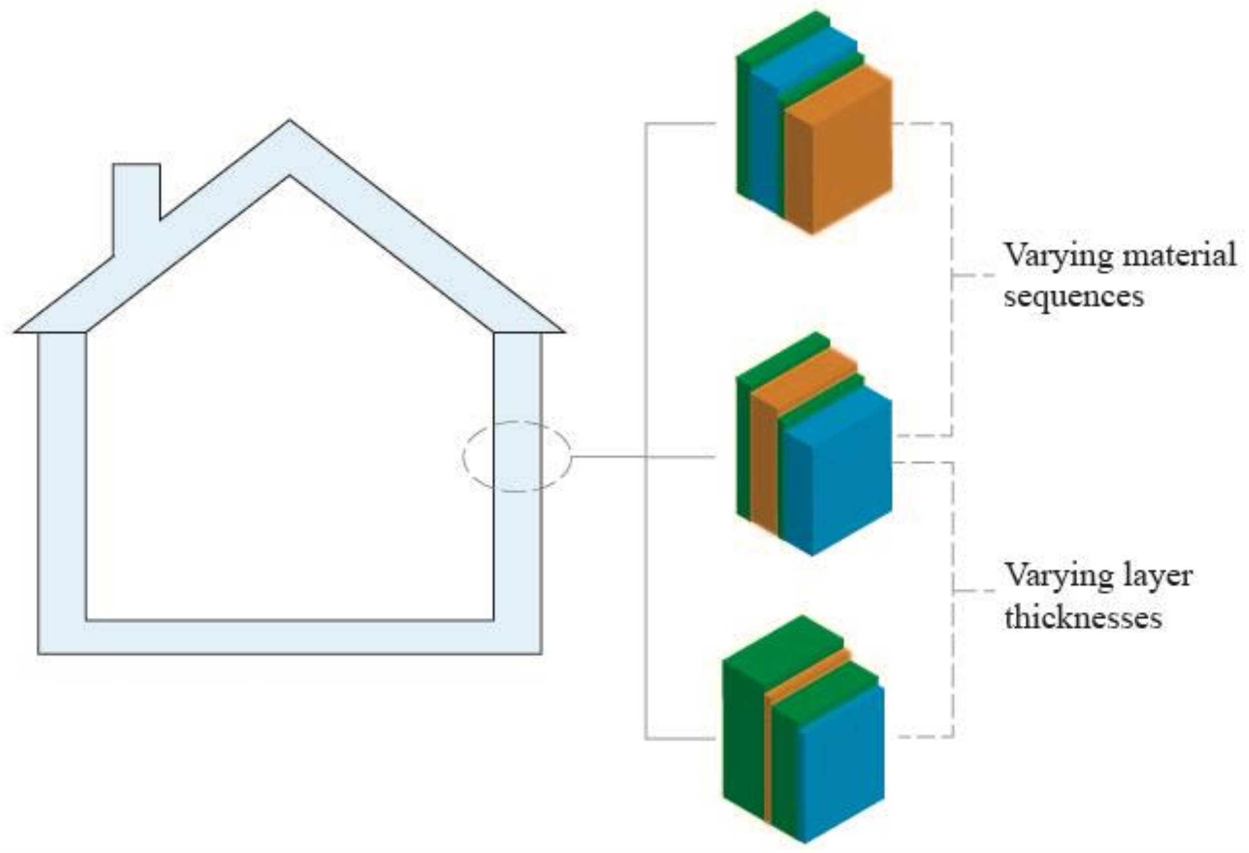
To summarize, and based on the studies of [24,25,26,27,28,29], the positioning of PCM in building envelopes is a challenge in terms of optimization, and the reported results are not always consistent. For example, Jin et al. [24] concluded a specific and optimized distance to the PCM layer’s temperature variation (external) side. Based on experiments Gounni and Alami [25] concluded that the PCM layer needs to be located next to the temperature variation side to assure a complete transition. Similar conclusions were drawn from simulations by Heim and Wieprzkowicz [29], who concluded that the PCM layer should be at the external wall. By contrast, Zhu et al. [28] concluded that the PCM layer should be located nearest the internal wall, far from the temperature variation side. The temperature over the envelope gradually changes over the wall thickness, and this temperature gradient might be more than 40 °C from the outside to the inside in wintertime in northern countries, with a daily variation. Thus it is essential to select a PCM with a transition interval to match the temperature and overlapped variation at that specific position in the wall. Suppose the PCM is positioned at wall temperatures out or partly out of the transition range. In that case, it will not fully contribute to the heat buffering at daily variations in the outside temperature. However, if temperature variation occurs inside due to electrical equipment or heating from humans, another match and strategy have to be considered. Therefore, the sequencing of the PCM layer in building envelopes needs further investigations and thickness dependency, shown in principal in Figure 1. Additionally, a well-established computational tool is required to support the design, which would be valuable when guiding, evaluating, and optimization PCM wall configurations.
The scope of this study is to introduce and validate a numerical approach to evaluate the influence on the thermal performance of a building envelope by sequencing PCM layers. Also, it concerns the question raised above: where should the PCM layer be located? The proposed approach is a finite element method (FEM), developed from a preliminary model introduced in [30] to simulate heat transfer performance of the building walls with PCM layers. Other researchers have previously studied FEM for building structures with a constant phase element. In this study, the FEM model is developed for the building construction incorporating phase change materials. For validation, the study includes an experimental study performed in a hotbox setup. The model introduced in [30] has been further improved in this study to obtain a better prediction for experimental results. Furthermore, an air gap and sub-cooling have been noticed, which is extremely important for further study. Also, a further extension has been made, including heat flux discussion.
The organized of the structure of this paper is as follows. First, in Section 2, the ex-FEM tool simulates PCM walls’ heat transfer and temperature profiles. Also, it introduces the experimental setup and materials used in the study. Then, in Section 3, the model is validated in three ways: (1) comparison with an electrical circuit analogy model presented by Gori et al. [31]. The comparison is based on the same parameters introduced in [30], including the same temperature profile, although not considered in the preliminary study as shown in [30]; also, the same materials; (2) it is validated with a results comparison with a COMSOL model; and (3) it is validated with the experimental data, followed by a summary of the model validation. In Section 4, a proposed following step study has been presented, and some preliminary results. Finally, in Section 5, a discussion of this study and some recommendations are given.
2. Methods
An explicit FEM is used to analyze the heat transfer through a wall, based on the one-dimensional heat transfer equation,
where T is the temperature, and k is the thermal conductivity, ρ is the material density, and cp refers to the specific heat capacity.
2.1. Numerical Method
2.1.1. Explicit FEM Approach
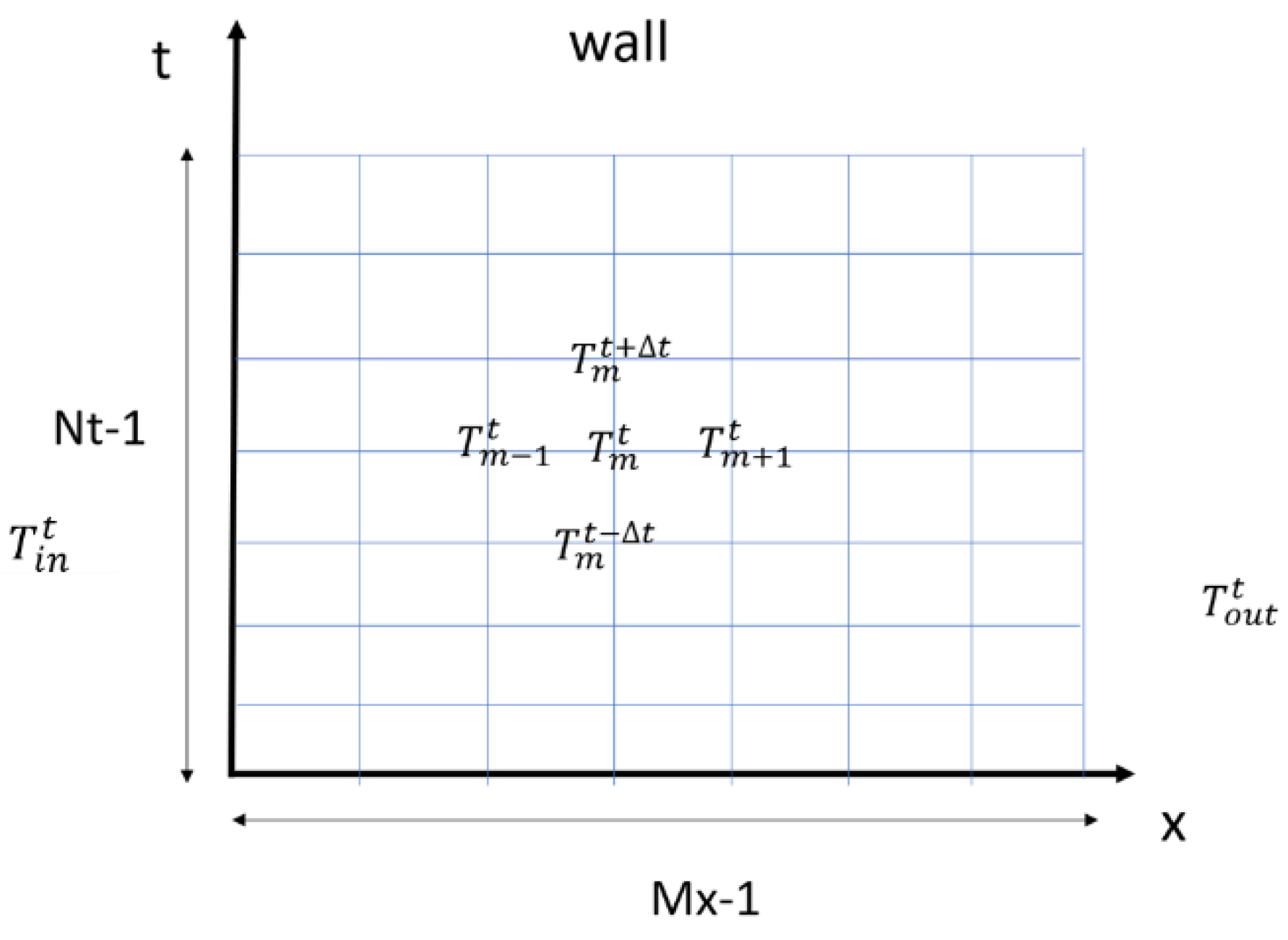
Figure 2 shows the general working procedure of the explicit FE-method. The x-axis is along with the wall thickness, while the y-axis is time. The temperature () at time step t + ∆t is derived directly from the temperature () at the previous time step t. The wall is discretized into Mx-1 elements from the inside to the outside. For convergence, the element size is 1 mm along the x-axis and 0.001 s along the time-axis in this study.
For element 1, at the inside wall boundary, the heat transfer equation is expressed as,
The inside air temperature of the box () follow the experimental values received in the hotbox study. The heat transfer coefficient at the inside surface () in the model simulation is obtained by numerical calibration, in the adjustment of the simulated temperature data at the internal wall to the experimental temperature data.
For the element Mx-1 at the outside boundary, the heat transfer equation is,
The outside air temperature () is a constant value, 23 °C. The value of the heat transfer coefficient on the outside () is also adjusted to follow the experimental data of the outside wall.
Regarding the in-between elements, the equation is,
2.1.2. Wall Configurations Studied
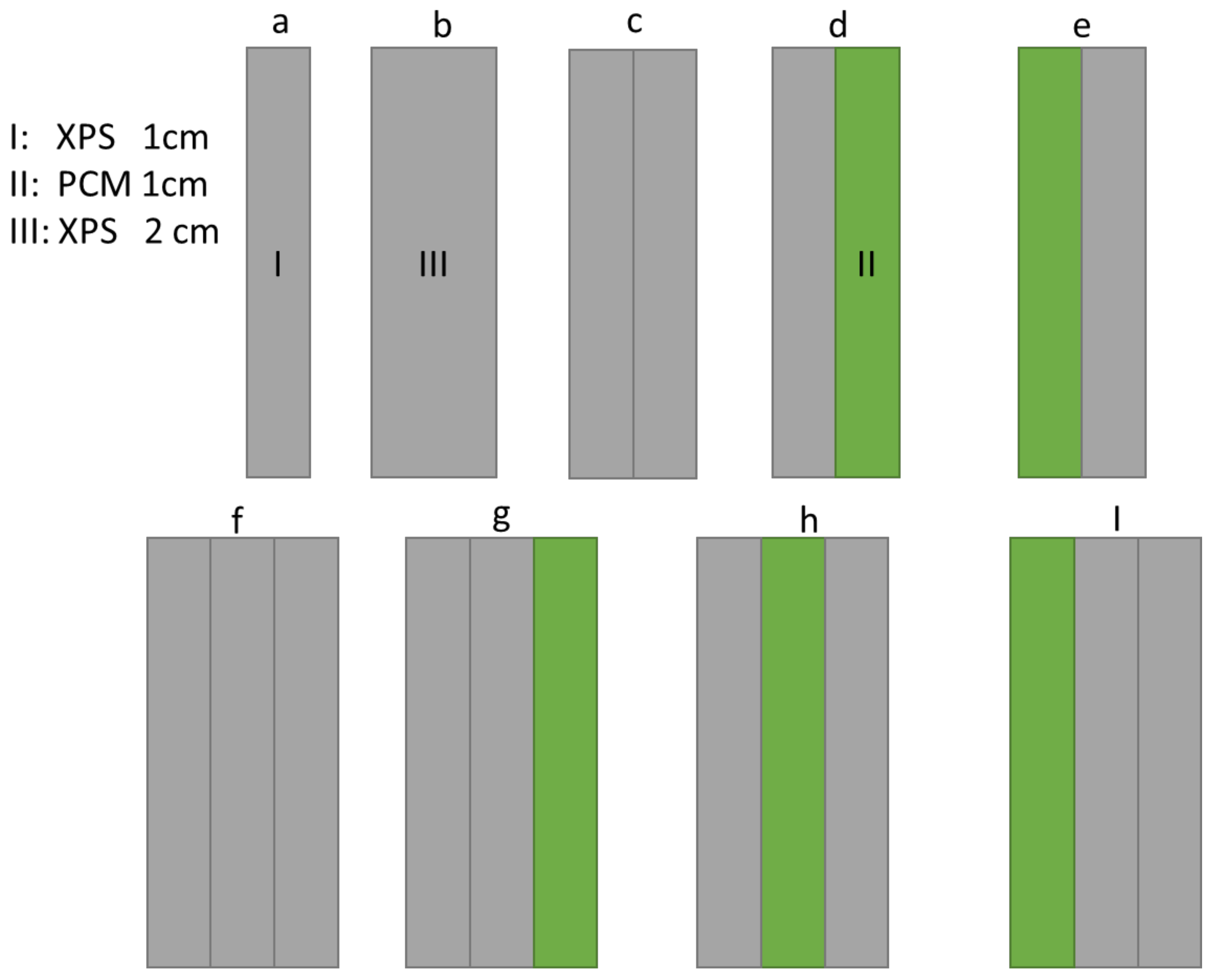
The wall configurations analyzed in this study are in Figure 3, illustrated from a to I. I (grey) is extruded polystyrene (XPS) layer of 1 cm: II (green) is PCM layer of 1 cm: III (grey) is XPS layer of 2 cm. The left side of the wall is the inside of the hotbox, where the temperature is regulated. The right side of the wall is the outside of the hotbox (the office room).
As Figure 3 shows, the experiments include three parts: one layer: a and b; two layers: c (XX), d (XP), and e (PX); three layers: f (XXX), g (XXP), h (XPX), and i (PXX) where P stands for PCM, and X stands for XPS. The sequence of the characters stands for the location of different materials. XPX, for instance, means XPS-PCM-XPS. The location of the PCM layer in the wall varied in the cases of two-layer and three-layer.
2.2. Lab Tests
For validating the accuracy of the explicit FEM model, the study used the small-scale experimental hotbox setup. This section also presents and discusses the experimental method, materials used, and the model validation results.
2.2.1. Experimental Setup
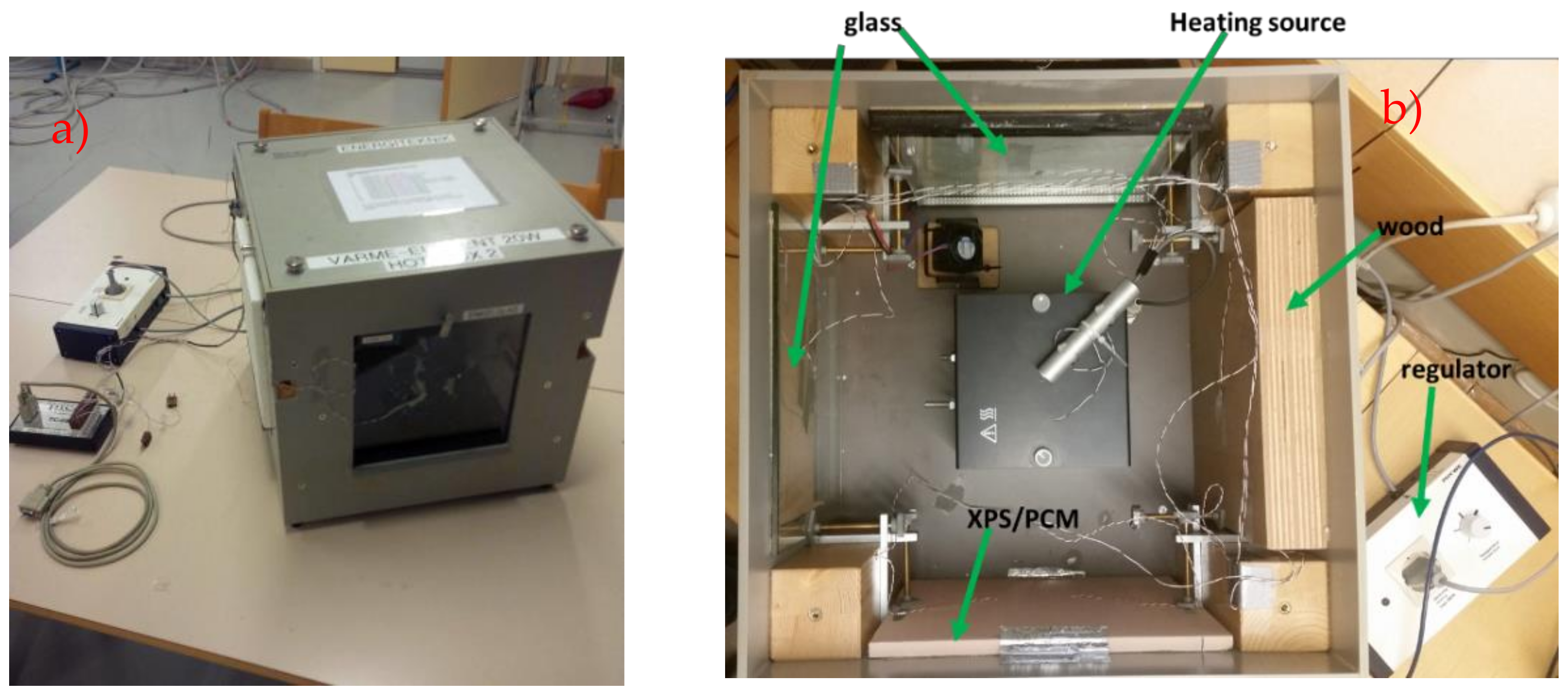
Figure 4a shows the hotbox with a L × W × H as 40 cm × 40 cm × 37 cm. The hotbox has four interchangeable wall Sections of different materials: styrofoam, wood, single glass, and double-glazed window. In this study, different wall layer configurations replaced the styrofoam wall, showed in Figure 3. All other walls were unchanged, as shown in Figure 4b.
The hotbox was located in an office room with an air temperature at approximately 23 °C, and a daily temperature variation of less than 1 °C. It was measured before the experiments were performed. Thus, the experimental conditions were limited to room temperature at around 23 °C as our lowest experimental temperature. The inside temperature of the hotbox was controlled by a regulator attached to a cylinder on the top of the black heating unit. The heating unit was located in the center of the hotbox to ensure a uniform distance to all surrounding four side surfaces. The temperature could be controlled and set within a range from room temperature up to a maximum of about 60 °C, depending on the actual heat losses through the walls. In this study, a maximum inside temperature was set close to 40 °C, which was reached when steady-state heat transfer conditions were achieved.
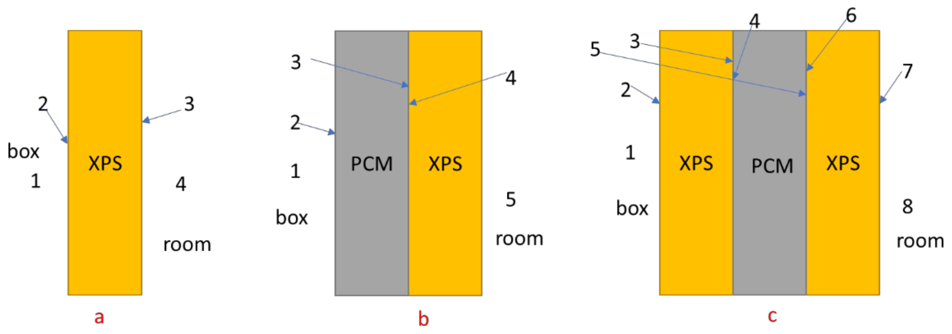
The temperatures at different positions and depths in the wall were measured by using type T thermocouples. The locations of the measured temperatures, numbered from the inside of the box for one layer, two layers, and three layers, are shown in Figure 5. The indication of the numbers of Figure 5b is taken as an example: (1) at the inside of the box in the air space at a half distance between the heating unit and the wall, (2) on the inner surface layer, (3) on the inner layer but the surface facing the outside of the box, (4) on the outer layer but on the surface facing the inside of the box, (5) on the outside layer on the surface facing the outside of the box, (6) in the air at a 5 cm distance from the outside surface facing the office. In the simulation, points 3 and 4 are considered one location, which is defined as a contact surface, and the contact surface properties are taken as a mixture of XPS and PCM. For three layers of Figure 5c, point 3 and point 4 are combined, and point 5 and point 6 are integrated into the simulation.
In a test, vertical air temperature gradients of about 6 °C were detected inside the box. To ensure a good air mixing and a uniform temperature distribution, a 40 mm × 40 mm fan was placed inside, not shown in Figure 4. It reduced the temperature gradient to less than 0.5 °C. All the thermocouples were connected to a Picolog TC-08 data logger associated with corresponding software and connected to a PC.
2.2.2. Materials
The investigated materials are XPS and PCM, and their properties are given in Table 1. The XPS was purchased from Sundolitt AB, and the PCM is Climsel 28 was purchased from Climator Sweden AB.
For PCM, the density and the thermal conductivity are considered to have constant values in each phase. For the specific heat capacity, a continuous function is used.
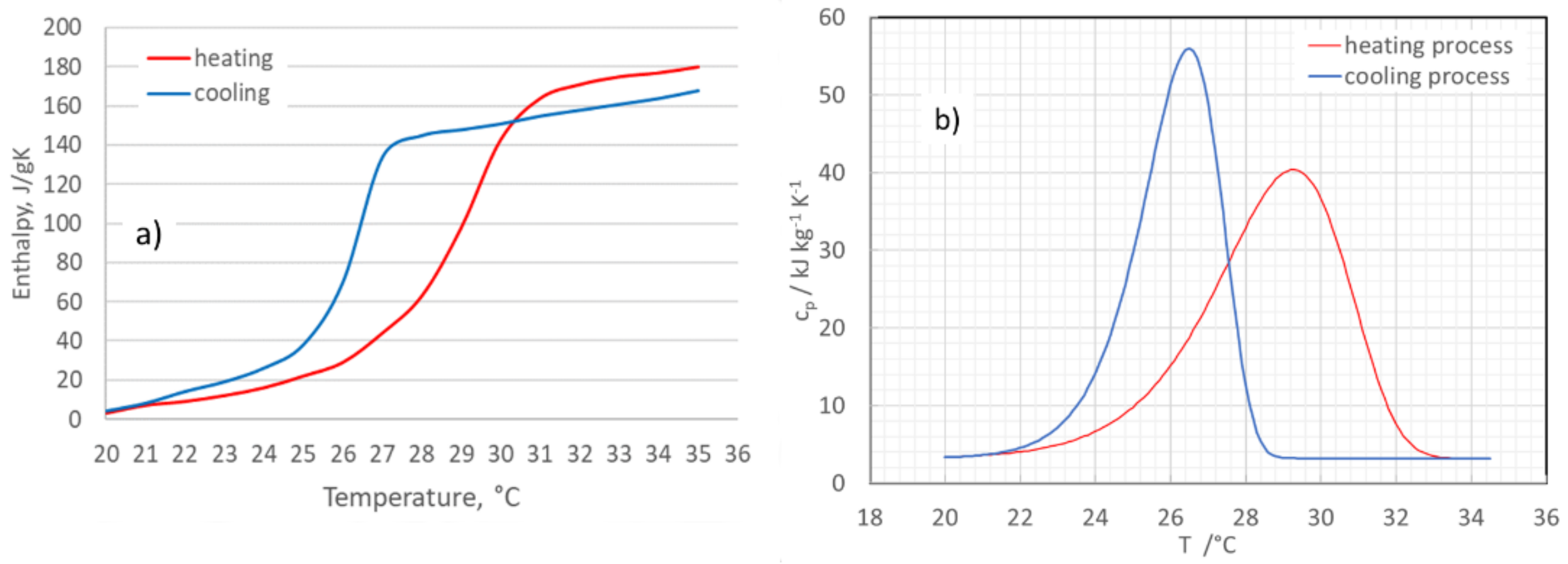
The specific heat of PCM is derived from the enthalpy data received from the PCM provider (Figure 6a). The enthalpy data is firstly integrated by a Weibull2 function, with parameters shown in the figure and a residential square of 0.99137. Then the derivation of the Weibull 2 function is derived as the cp function as Equation (5). The area under the cp-curve reflects the latent heat of the PCM transition (shown in Figure 6b).
For heating process: a = 176.6311, b = 8.32946, d = 17.59206, k = 0.03406.
For cooling process: a = 156.9963, b = 10.43071, d = 25.94152, k = 0.0377.
Figure 6 shows that the PCM material has a phase transition starting at about 23 °C and ends at about 32 °C in the heating process, with a transition maximum close to 29 °C. While in the cooling process, the transition starts at about 29 °C, which is about 3 °C different from that in the heating process. This is called a sub-cooling phenomenon of the phase change materials.
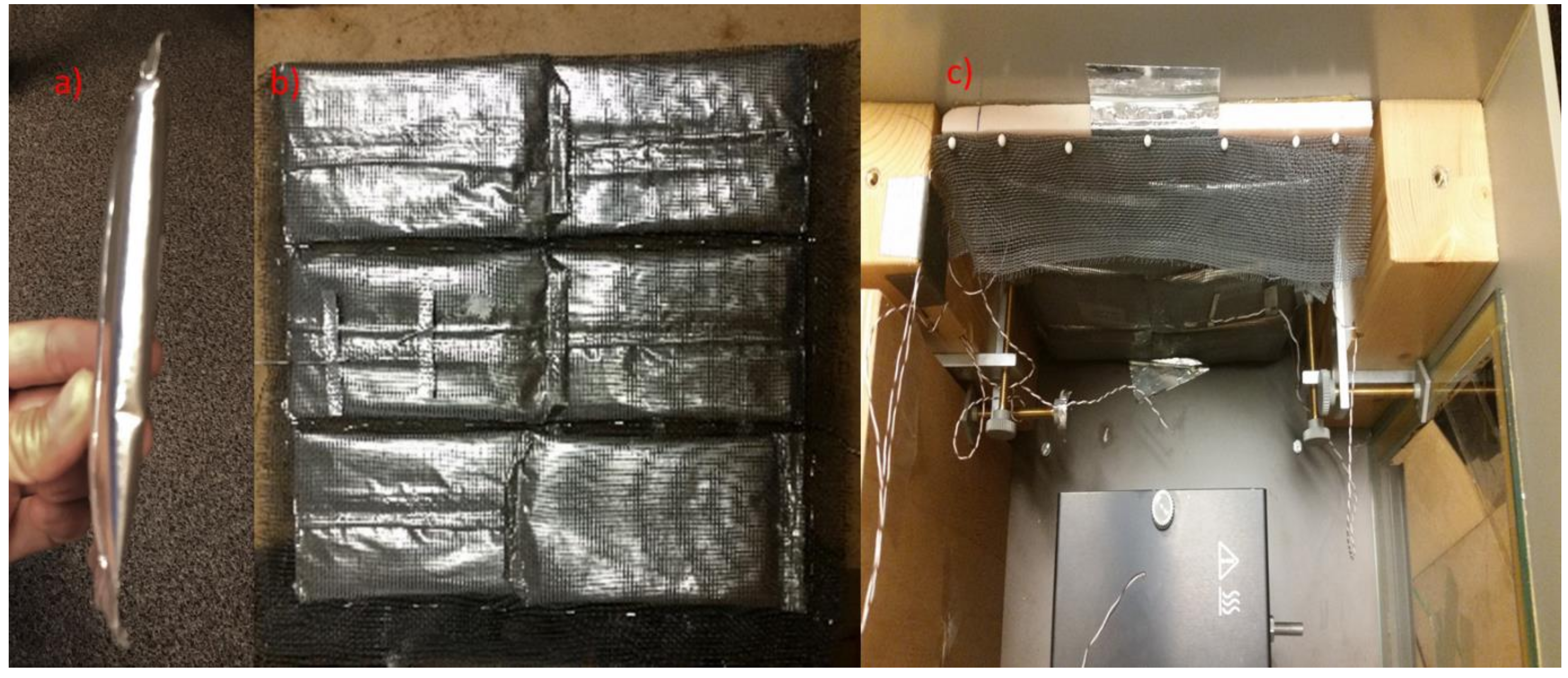
The PCM material purchased is packed in small bags of size 7 cm × 12 cm and a thickness of about 1 cm, as shown in Figure 7a. Six of the bags were enclosed in a thin polymer net (as shown in Figure 7b). Some of the edges are overlapping to reduce the effects of air gaps, which will result in inhomogeneous heat transfer through the surface, which will be discussed in the result Section below. Tiny needles pin the net onto the XPS wall (Figure 7c) in the two-layer experiment. In the simulations, the netted PCM bags were modeled as a uniform PCM layer, with an equivalent thickness of 1 cm.
3. Results
3.1. Validation of the Model with ECA
The explicit FEM model is verified by comparing the obtained results with the results obtained by using the electrical circuit analogy model introduced by Gori et al. [25] for the wall configurations of d and e in Figure 3.
In the electrical circuit analogy (ECA) method, the heat flow corresponds to the electrical current. Gori et al. [25] used that method and sequenced insulating and thermally conductive layers. In our study, the XPS material is considered the insulation (I) layer, while concrete/steel is regarded as the conduction (C) layer. The temperature variation side for the model verification is on the room side. Therefore, Figure 3d corresponding to IC (insulation/conduction wall configuration, with temperature variation in the insulation side) mode, while Figure 3e corresponding to CI (conduction/insulation wall configuration, with temperature variation in the conduction side) mode, discussed in the later text in this Section. In our comparison of the two methods, we have used the same material properties as Gori. For the insulating I-layer, we used thermal conductivity λ = 0.034 W/mK, thermal diffusivity m2/s; and for the C-layer thermal conductivity λ = 0.81 W/mK, thermal diffusivity m2/s. More details about the electrical circuit analogy method can be found in [25].
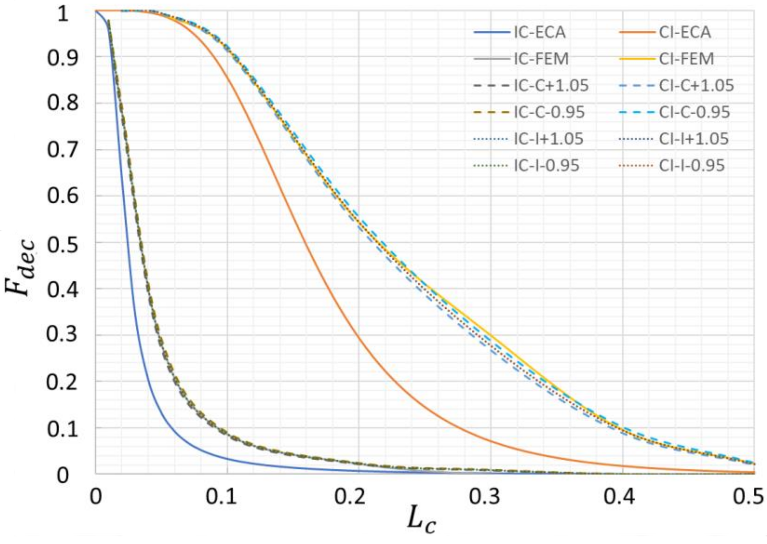
Figure 8 shows the results from both ECA and FEM. Fdec in y-axis is the temperature decrement factor defined as . and are the temperature variation amplitudes on the internal and external surfaces of the wall. Lc in the x-axis is the thickness of the conduction layer. The ratio of Lc and the total thickness of the wall is 0.5. For FEM, the inside temperature is set to 23 °C, while the outside temperature is set to a sinusoidal function as , where w is the angular frequency ω = 2π/T = 7.27 · 10−5 rad/s for one day. The external heat transfer coefficient in the FEM-model is set to be an extremely high value () to obtain an external surface temperature that follows To. The internal surface temperature variation is then obtained based on Equations (2)–(4) by using adiabatic boundary conditions, setting hi = 0. The sensitivity of the conduction and the insulation layer property () on the temperature performance of the decrement is also analyzed and shown in Figure 4. IC-C + 1.05 denotes that for the wall configuration IC mode, with conduction layer property a deviation of +5%; IC-C − 0.95 (−5%) denotes that for the wall configuration IC mode, with conduction layer property a deviation of −5%; IC-I + 1.05 denotes that for the wall configuration IC mode, with insulation layer property a deviation of +5%; IC-I − 0.95 (−5%) denotes that for the wall configuration IC mode, with insulation layer property a deviation of −5%; the validation was the same for the CI mode.
The results indicate a qualitatively good agreement between the two models, where the trends are quite the same. The difference in the results of the IC mode is quite small, while the results for CI mode give a relatively large deviation with a conduction layer thickness larger than 0.15. Figure 8 also shows that the property combination ) has a minor influence on the temperature decrement factor (within ±5% deviation, the change of Fdec is ignorable).
3.2. Validation of the Model with COMSOL
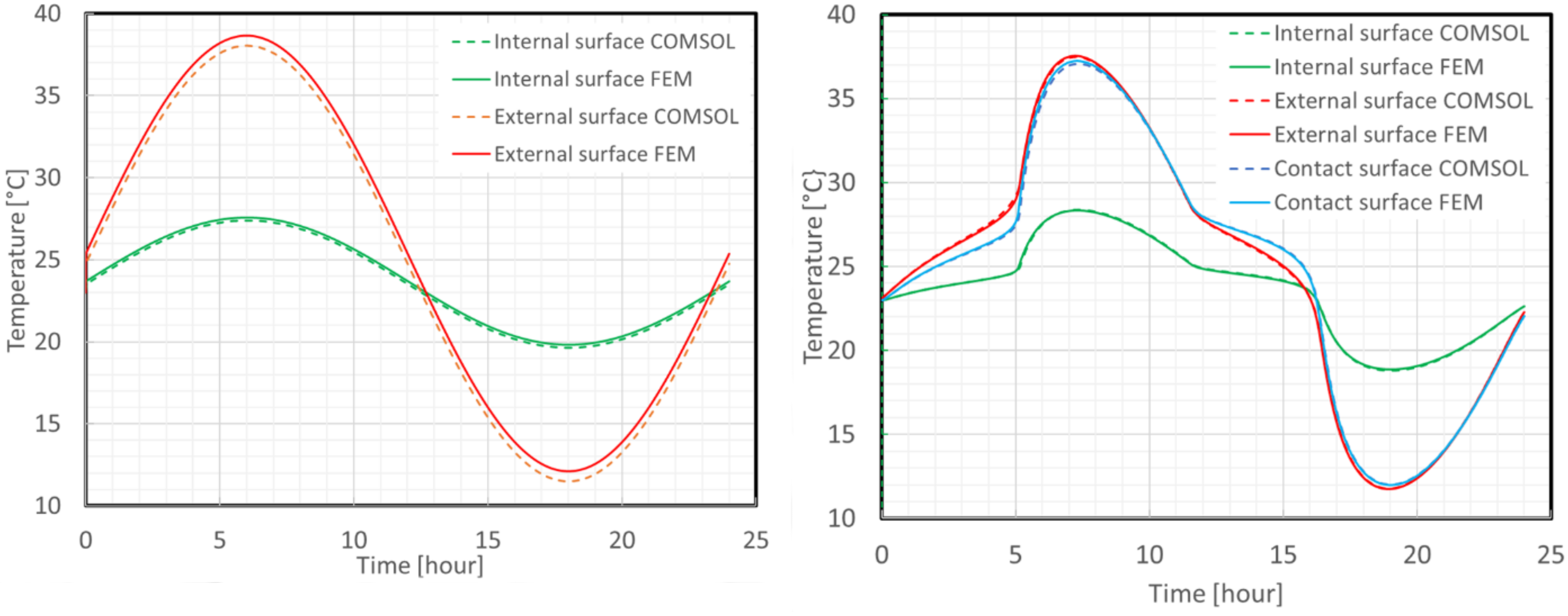
Baghban et al. (2010) [32] have utilized a COMSOL model to simulate a wall system with high-performance materials and concluded that COMSOL Multiphysics has a high potential for building physics simulation tools. This study also uses a COMSOL model to validate the FEM model with wall configurations of a and e shown in Figure 3. A temperature variation of as has been applied. Figure 9 shows the comparison of the results from both FEM and COMSOL. The root mean square between FEM and COMSOL for external and internal surfaces ( ) show the deviation and listed in Table 2, which indicates a good match between the two models regarding the temperatures in different surfaces.
3.3. Validation of the Model with Experimental Data
3.3.1. One Layer (Configurations a and b)
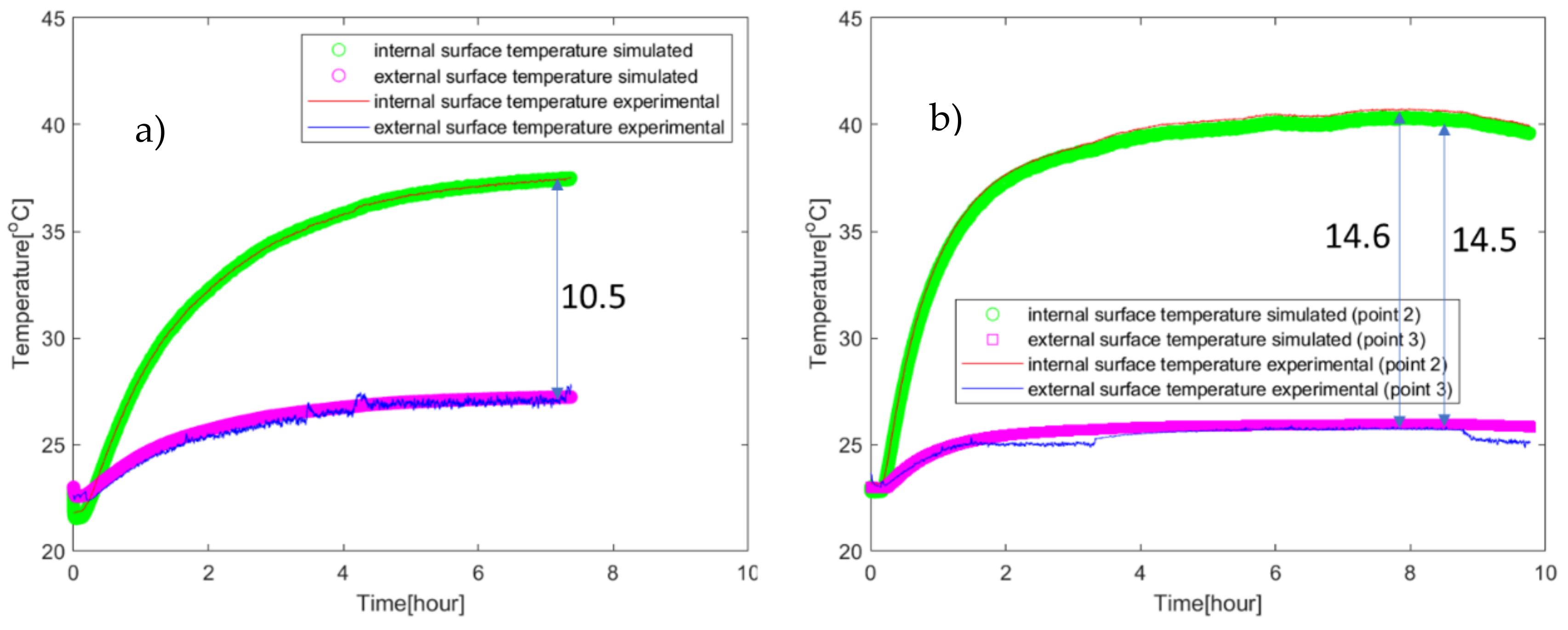
For configuration a, i.e., the 1 cm thick layer of XPS, the results are shown in Figure 10. The data of both the experimental and simulated temperatures obtained at the inside and outside surface. With these two surface temperatures, the inside surface convection coefficient and the outside surface convection coefficient was calibrated. The coefficients are adjusted until we get the best match between the two data sets () and (). Using the difference between the data sets, the root mean square error (RMSE: ) was calculated.
The matching procedure gave a = 18 W/(m2K) and a As shown in Figure 10a, there is a very good match between the simulated and experimental temperatures received in the 1 cm XPS case. = 5.5 W/(m2K), with an RMSE of 0.17 °C and 0.21 °C for the two temperature differences, at the internal and external surfaces, respectively. As expected, we obtain a higher convection coefficient inside the box due to the forced convection of the fan. A comparison was also made with the same convection values for the 2 cm XPS case, i.e., configuration Ib, giving a small increase in the RMSE values to 0.32 °C at the internal surface and 1.27 °C at the external surface respectively, see Figure 10b. In the latter case, which did not happen in case Ia, we see a minor influence in the experimental measurements of the ventilation system in the room turning on and off, expected to have a minor effect on the convection at the external surface of the box, giving a higher RMSE. The good correspondence of the temperature profiles indicates that the simulation tool (ex-FEM), applied in this study, can predict the experimental results well in the XPS cases.
The maximal internal surface temperature of the XPS changes from about 37.8 °C in Figure 10a to 40 °C in Figure 10b. At the same time, the temperature at the outside of the XPS layer is also somewhat lower in the latter case, which indicates better isolation due to a thicker isolation layer. However, due to differences in heat flow, the temperature drop over the wall is not doubled, as might be expected when the wall thickness increased from 1 cm to 2 cm. Thus, the actual temperature drop ratio is 14.5/10.5 = 1.38 in the simulation and 1.39 in the experiment.
3.3.2. Two Layers (Configurations c–e)
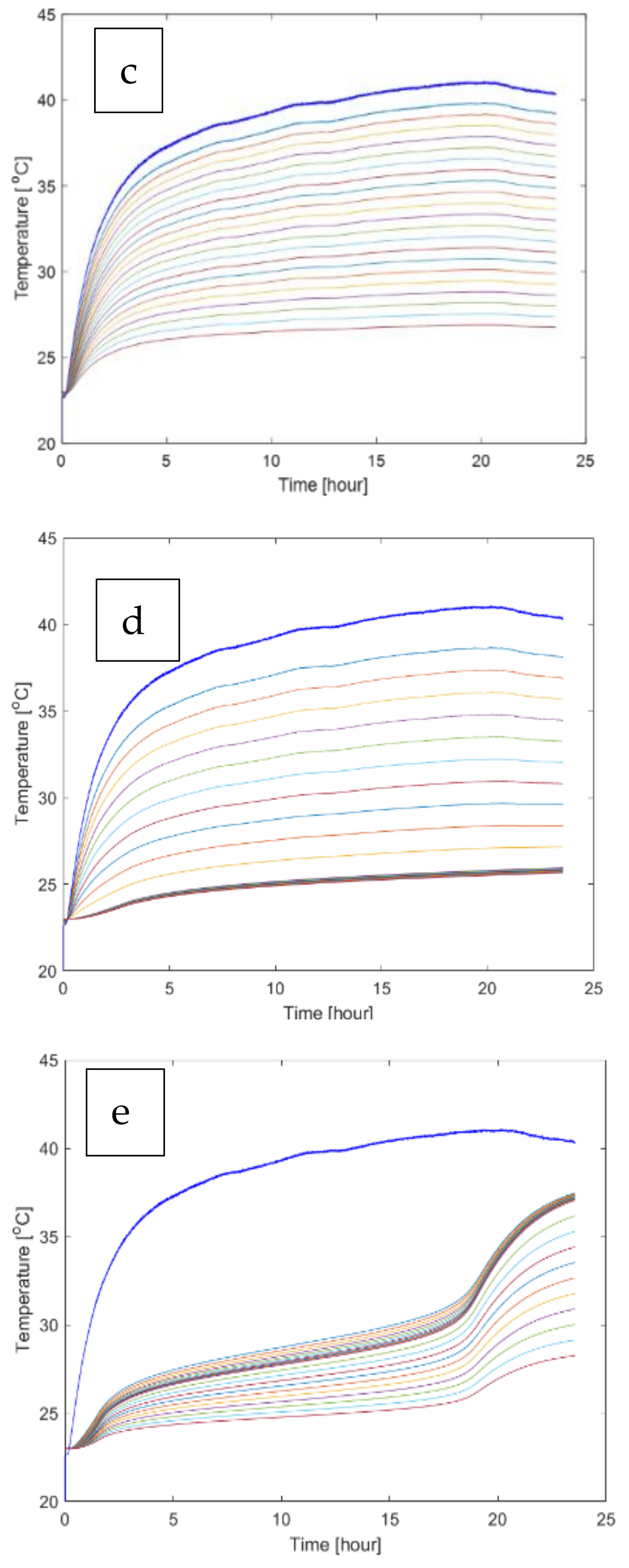
The two-layer configurations c–e are shown in Figure 11, respectively. Each curve in the figure represents a temperature profile at different tenths of the total thickness of each layer in the wall. The blue curve in Figure 11 is the air temperature inside the hotbox, which indicated the temperature variation profile. Due to much higher thermal conductivity in the PCM compared to that in the XPS, the curves of the PCM will lump together, which can be noticed from the comparison of the wall configurations of XX with XP and PX.
When the PCM layer is in the outer position, as in configuration d, the temperature of the PCM will just reach the lower temperature range of the phase transition. The start of the transition is partly observed at about 24 °C, where the initial temperature rise is held back to the highest temperature of about 26 °C. However, the transition is still not completed at this temperature, and in that case, the storage capacity is not entirely used. In configuration e when the PCM layer is at the inner layer, the temperature of the PCM will pass the transition range, and is in Figure 11 e-PX observed at about 30 °C where the temperatures start to rise more rapidly again. Therefore, hotbox experiments were only conducted for the case of wall configuration e.
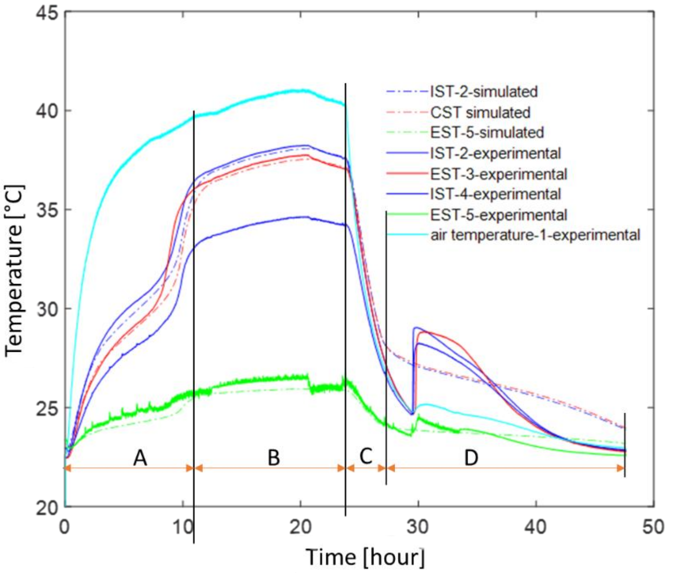
The comparisons of the temperature profiles from experiments and simulations for the two-layer configuration e, are shown in Figure 12. The uppermost temperature profile is the measured air temperature inside the box for the heating process, increasing quickly. Both simulated and experimental temperatures on the PCM layer and the XPS layer show a fast increase which is slowed down after about 2 h when the transition in the PCM starts. This transition ends after about 10 h, which gives a sharp rise in the temperatures and levels out at relatively constant values when steady-state conditions in the heat flow are reached.
The contact surface temperature from simulation follows almost the same pattern (turning points are almost at the same condition) as the experimental measurement at EST-3 during the heating and steady-state process as it shows in Figure 12. At the same time, it shows a big difference compared to the experimental data at point 4. For simulation, the temperature at the contact surface is calculated based on a combination of the properties of PCM and XPS. Due to the high thermal conductivity of PCM, the simulated contact surface is more similar to PCM. Thereby, the CST-simulated follows more with EST-4. Another reason for this can be an unpredictable thermal resistance between point 3 and point 4, which is not considered in the simulation.
For the cooling process (from 23 h to the end as shown in Figure 12), the air temperature decreased from about 40 °C to 25 °C quickly in the beginning (in about 5 h), then slowly to 23 °C within about 17 h. The internal surface temperature from the experiment decreased from 37.8 °C to 25 °C, followed by a sudden jump to 29 °C, and then reduced to 22.9 °C in the end. The sudden jump is caused by a partial, about 7%, release of latent heat due to a subcooling of 4 °C. With a corresponding and successive heat release, the solidification process is ongoing for about another 15 h. The simulated temperature results at the internal PCM surface in Figure 12 show a decrease from 40 °C to 29 °C in the first 5 h and a smooth reduction to about 23 °C at the end of the measurements.
The sudden temperature increase observed in the experimental data is not noticed in the simulation. The reason is that the subcooling effect of the PCM is not considered in the simulation.
The heat convection inside and outside the layers and matching the heat transfer coefficients is not straightforward. Here we have found that hi = 18 W/(m2K) and ho = 13 W/(m2K) gives a reasonably good match with the experimental results (for the values, see Table 3).
The whole process consists of four periods (A–D). Period A is the heating process before steady-state; Period B is the steady-state period. Period C is the cooling process before sub-cooling happened; Period D is from the sub-cooling moment to the end of the experiment. The R-value for period D is excluded. It is because sub-cooling induces a large deviation. It shows in Table 4 that there is a small deviation ( are 0.019 and 0.028 for IST and CST) when a steady-state. The maximum deviation is on the contact surface in the heating process (with a of 0.965, caused by the phase transition, which can induce extra thermal resistance between the two contact surfaces. The external surface shows a quite good match during the whole process, as indicated by the root mean square value (0.184).
3.3.3. Three Layers (Configurations f–i)
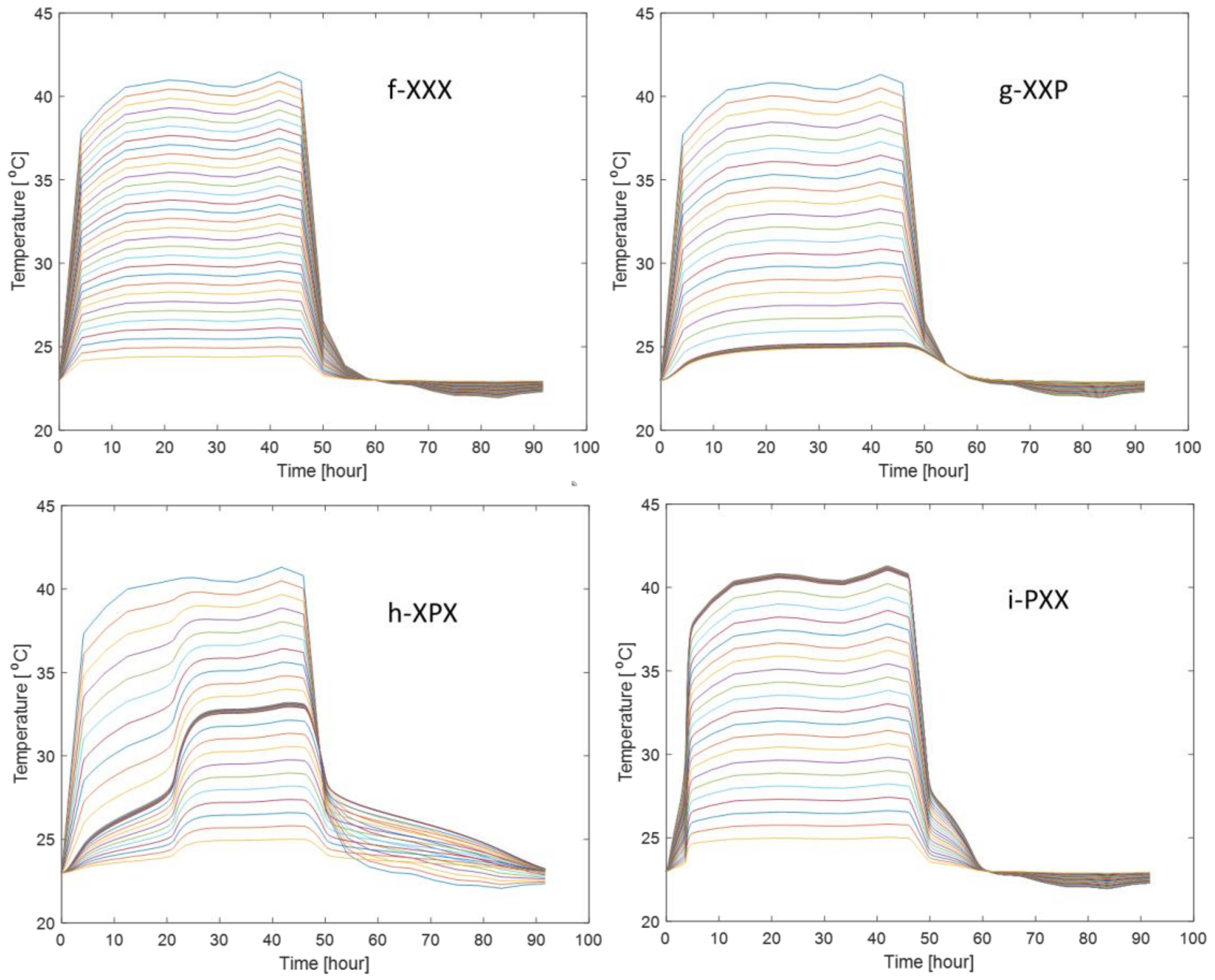
Simulation results of the three-layer wall configurations f–i are shown in Figure 13. These indicate that for the PCM layer located in the middle of the XPS layers, the PCM layer works the best for this study conditions. For the case of XXP, when the PCM layer is on the outside, the PCM cannot be activated. For PXX, the amount of PCM is not enough, then the temperature still increases/decreases fast during the heating and cooling process. The external surface maintains a relatively higher temperature in a longer period during the heating process and a lower temperature during the cooling process. Therefore, only the wall configuration h-XPX was performed for the experimental study.
The comparison of the experimental and the simulation results of wall configuration h-XPX are shown in Figure 14. For the heating process, the air temperature inside the hotbox increases rapidly to about 40 °C and then slightly increases and maintains a temperature of about 41 °C before cooling starts. The internal surface temperature from the simulation does not show a phase transition from the two contact surfaces and the external surface temperature. The phase transition from the simulation and experiment is not the same as for the two-layer wall configuration shown in Figure 12. The phase transition from simulation and experiment started at almost the same time. Nonetheless, it ended earlier in the simulation (period c), at about 12 h with a temperature of 28 °C, while experimental results showed an end at about 27 h with 29 °C (period d), possibly caused by an extra thermal resistance between two surfaces challenging to control in simulation.
The cooling process started at about 48 h, indicating a rapid decrease in the air temperature. The air temperature dropped to 25 °C within about 2 h and then decreased to 23 °C within about 10 h. The contact surface temperature at points 3–5 from the experiment followed the decrease to about 26 °C and then showed a jump, which is the same as shown in Figure 12, caused by a partial release of latent heat subcooling of about 3 °C. After that, it decreased to a final temperature of 23 °C. This phenomenon of a temperature jump was not noticed in the simulation, which is for the same reason as for two layers.
The value between the experimental and simulated results is shown in Table 4 for the internal and external surfaces. The big difference between the contact surfaces has been discussed for uncontrolled thermal resistance problems. Compared with two layers configuration e, three layers configuration h has a thicker wall in total, which can give a higher air velocity inside the hotbox, then a higher can be expected. Therefore, Figure 14 is derived based on a , and then a relatively good match can be obtained as shown in Table 4.
3.4. Short Summary on the Validation
According to the previous Sections, to be trustworthy when simulating building performance incorporated with PCMs, the FEM model has been validated. However, the comparison of the FEM and experimental results indicates that several parameters need to be considered. There are difficulties in controlling the system when conducting experiments. The heat convection must be measured to obtain a reasonable value in the simulation. Also, the thermal resistance between two contact surfaces, when PCMs are applied especially, is difficult to predict. Therefore, more studies are needed to check the usability of the model. Also, the sequencing of PCM layers in the wall configurations needs further investigation with more complexities.
4. Proposal of Future Work
Based on the validation of the model above, in this section, further steps were taken. With the complexity mentioned in 3.4, the adiabatic boundary for the external surface was introduced.
The analyzed system in this Section was a room with an ambient temperature variation as , with a maximum temperature of 40 °C, and a minimum of 10 °C. The wall analyzed comprised XPS and PCMs, which were the same as mentioned above, in different combinations.
4.1. Advantage of Using PCM
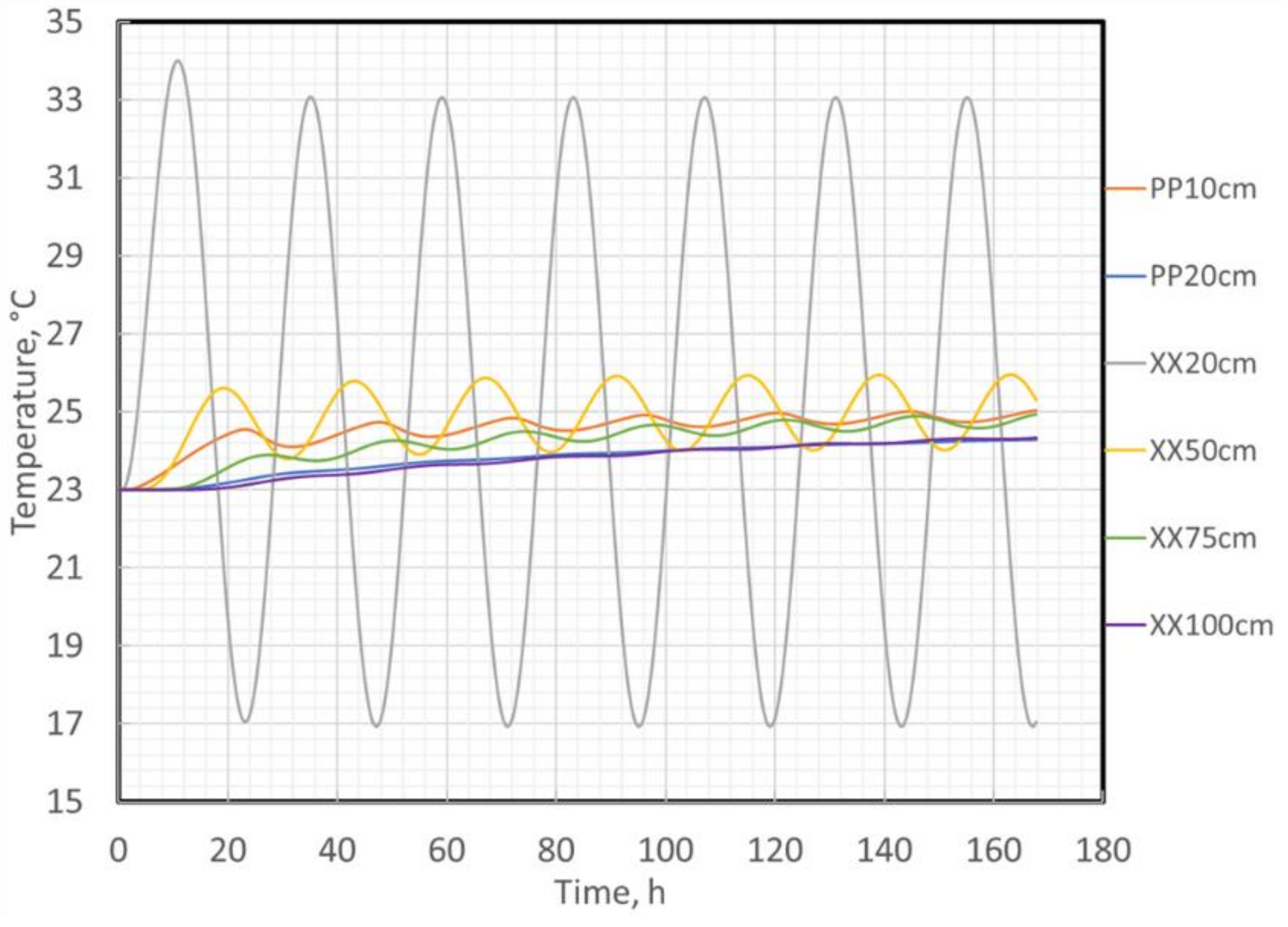
Figure 15 shows the result of the internal temperature variation with different wall materials and thicknesses. For example, in the legend, PP10 cm represents two layers of PCM with a total thickness of 10 cm; XX20 cm stands for two layers of XPS with a total thickness of 20 cm.
Figure 15 shows, with a wall configuration of PP10 cm, that the internal surface temperature varies during the period by about 1 °C. However, a wall configuration of XX20 cm shows a significant variation of the internal surface temperature (17 °C during the period). With a wall configuration XX75 cm, a similar variation with that of PP 10 cm, was achieved. Additionally, wall configurations of PP20 cm and XX100 cm result in a more stable internal surface temperature.
According to Figure 15, it is possible to achieve a stable inside room temperature with an ambient temperature variation of 30 °C (10~40 °C). A five-times thinner wall is needed when only PCMs are applied.
4.2. PCM Location
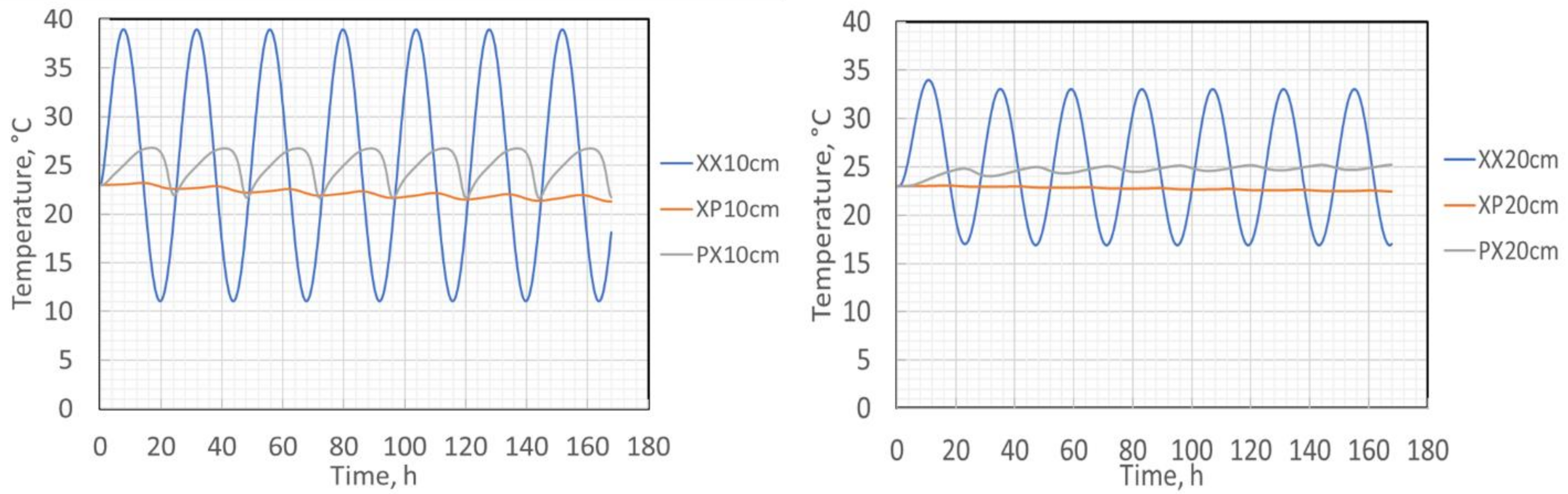
For a two-layer wall configuration, the internal surface temperature comparison of XP and PX, a comparison is shown in Figure 16. It illustrates that without PCM, XX10 cm, the temperature follows the ambient temperature. While a PCM layer replaces one XPS layer, the temperature variation is less with the PCM layer located next to the room side. In addition, the total wall thickness for all situations is the same.
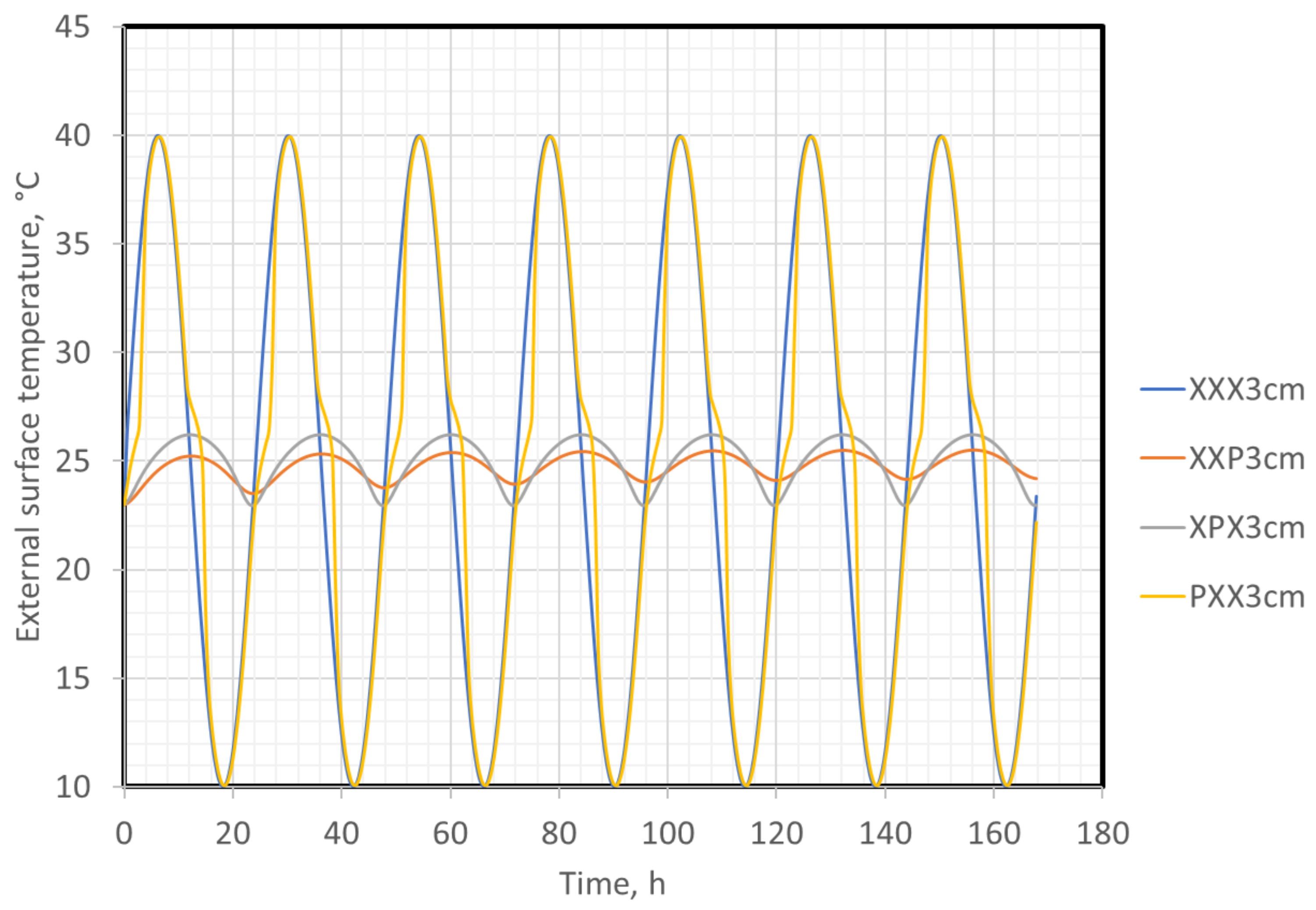
The result with a three-layer wall configuration is shown in Figure 17. It indicates that when the PCM layer is next to the room side, the wall system has a better temperature regulation, giving a much lower temperature variation when the same ambient temperature is applied, with fixed total wall thickness. It is the same as for a two-layer wall configuration, as shown in Figure 16.
4.3. Short Discussion
According to the results shown in Figure 16 and Figure 17, the PCM layer should be next to the room side, where there is a temperature stability requirement, consistent with some of the conclusions from other researchers [28]. However, this conclusion is based on this study’s assumptions, using a sinusoidal temperature variation. Additionally, the PCM layer has the same thickness as the other wall layer (insulation layer). Therefore, according to the results, it is suggested that more ambient temperature profiles, actual weather profiles primarily, should be studied later with further validation of the model and further understanding of the application of PCM wall systems.
5. Discussion
In experiments with a double thickness of the XPS wall layer, we do not observe a doubled temperature drop across the wall, attributed to a difference in heat flow. Therefore, the control system in the experimental setup needs to be improved, together with measurements of the heat flow, to adjust and select a specific heat flow in the different cases. Unfortunately, it has not been possible in this study.
Both the hotbox’s inside and outside heat transfer coefficients are essential factors in the simulations and adjustable to obtain a good fit of simulated temperature data to the experimental data. For example, an installed fan inside the hotbox to reduce temperature gradients gives us a higher heat transfer coefficient at the inside surface. In order to eliminate the influence of the heat transfer coefficient for the simulation result, a boundary temperature variation condition or a measured heat transfer coefficient value can be considered for further study.
There are possible unpredicted thermal resistances between the two contact surfaces to be considered. Also, due to phase transition, that effect can be regarded as unpredictable. Therefore, more layer splitting could be more challenging to control and predict. For example, Fantucci et al. [33] mentioned the possible air-pocket generation because of the volume shrinkage of PCM, which could be avoided by bending the alveolar polycarbonate container used to fill PCM. In a future study, we will further consider air pockets.
Subcooling was observed in the experiment, found to be relevant for consideration in the simulation model. Kuznik and Virgone (2009) [34] have experimentally measured the specific heat capacity of a composite PCM, and they pointed at the differences in the phase change temperatures received at heating and cooling. Hysteresis and subcooling effects are essential factors to be considered in future simulations. Kuznik et al. [35] developed a TRNSYS model based on the experimental data from [26], which gives a good agreement between the experimental and simulated results. Their study also emphasizes the importance of the different thermal properties received during the heating and cooling process. Fantucci et al. [33] also studied the specific heat at heating and cooling for two different PCMs, one organic paraffin and one inorganic salt hydrate. The latter showed a hysteresis effect in the transition temperature, while the first showed almost the same transition temperature at heating and cooling. Therefore, the selection of PCMs is also crucial, depending on the application.
With the validated FEM model, the study has shown the advantage of using PCM and analyzing the location. This study shows that the wall layer thickness can be reduced with PCM to achieve a stable room temperature.
6. Conclusions and Recommendations
An explicit finite element method (ex-FEM) has been verified and validated by other models and experimental data and found to be a promising tool for predicting the thermal performance of the simplified building walls when incorporated with phase change materials (PCMs). Furthermore, the study identified several unpredictable factors relevant for future studies.
The study included sequencing of PCM layers. The experiment illustrated how PCM could be either fully or partly melted when located next to the temperature variation side. Additionally, the simulations conducted indicated a more stable room temperature with PCM next to the room side. Consequently, there is evidence for the location of PCM to be regarded according to the requirement of the application.
Author Contributions
Conceptualization, H.Z. and T.O. and Å. Fransson; methodology, H.Z.; software, H.Z.; validation, H.Z.; formal analysis, H.Z.; investigation, H.Z. and Å. Fransson; resources, H.Z.; data curation, H.Z. and Å.F.; writing—original draft preparation, H.Z.; writing—review and editing, H.Z., T.O. and Å.F.; visualization, H.Z., T.O. and Å. Fransson; supervision, T.O. and Å. Fransson; project administration, T.O.; funding acquisition, T.O. All authors have read and agreed to the published version of the manuscript.
Funding
Northern Periphery and Arctic program, Kolarctic CBC Project: KO1089 Green Arctic Building; ERA-NET Smart Energy Systems and MICall19 project DEVISE- Different Energy Vector Integration for Storage of Energy.
Data Availability Statement
Data is available in the department of Applied Physics and Electronics, Umeå University.
Acknowledgments
The authors would like to thank the Northern Periphery and Arctic program, Kolarctic CBC Project: KO1089 Green Arctic Building, and the ERA-NET Smart Energy Systems and MICall19 project DEVISE- Different Energy Vector Integration for Storage of Energy, for the financial support.
Conflicts of Interest
The authors declare no conflict of interest.
References
- Hasnain, S.M. Review on sustainable thermal energy storage technologies, Part I: Heat storage materials and techniques. Energy Convers. Manag. 1998, 39, 1127–1138. [Google Scholar] [CrossRef]
- Hasnain, S.M. Review on sustainable thermal energy storage technologies, Part II: Cool thermal storage. Energy Convers. Manag. 1998, 39, 1139–1153. [Google Scholar] [CrossRef]
- Navarro, L.; de Gracia, A.; Colclough, S.; Browne, M.; McCormack, S.; Griffiths, P.; Cabeza, L.F. Thermal energy storage in building integrated thermal systems: A review. Part 1. active storage systems. Renew. Energy 2016, 88, 526–547. [Google Scholar] [CrossRef] [Green Version]
- Navarro, L.; de Gracia, A.; Niall, D.; Castell, A.; Browne, M.; McCormack, S.J.; Griffiths, P.; Cabeza, L.F. Thermal energy storage in building integrated thermal systems: A review. Part 2. Integration as passive system. Renew. Energy 2016, 85, 1334–1356. [Google Scholar] [CrossRef] [Green Version]
- Wang, X.; Zhang, Y.; Xiao, W.; Zeng, R.; Zhang, Q.; Di, H. Review on thermal performance of phase change energy storage building envelope. Sci. Bull. 2009, 54, 920–928. [Google Scholar] [CrossRef] [Green Version]
- Zhu, X.; Liu, J.; Yang, L.; Hu, R. Energy performance of a new Yaodong dwelling, in the Loess Plateau of China. Energy Build. 2014, 70, 159–166. [Google Scholar] [CrossRef]
- Uno, P. Concrete thermal mass and energy-efficient design. Constr. Rev. 1993, 66, 159–166. [Google Scholar]
- Goodhew, S.; Griffiths, R. Sustainable earth walls to meet the building regulations. Energy Build. 2005, 37, 451–459. [Google Scholar] [CrossRef]
- He, H.; Zhao, P.; Yue, Q.; Gao, B.; Yue, D.; Li, Q. A novel polynary fatty acid/sludge Ceram-site composite phase change materials and its applications in building energy conservation. Renew. Energy 2015, 76, 45–52. [Google Scholar]
- Athienitis, A.; Liu, C.; Hawes, D.; Banu, D.; Feldman, D. Investigation of the thermal performance of a passive solar test-room with wall latent heat storage. Build. Environ. 1997, 32, 405–410. [Google Scholar] [CrossRef]
- Ismail, K.; Castro, J. PCM thermal insulation in buildings. Int. J. Energy Res. 1997, 21, 1281–1296. [Google Scholar] [CrossRef]
- Wijesuriya, S.; Brandt, M.; Tabares-Velasco, P.C. Parametric analysis of a residential building with phase change material (PCM)-enhanced drywall, precooling, and variable electric rates in a hot and dry climate. Appl. Energy 2018, 222, 497–514. [Google Scholar] [CrossRef]
- Marin, P.; Saari, M.; de Gracia, A.; Zhu, X.; Farid, M.M.; Cabeza, L.F.; Ushak, S. Energy savings due to the use of pcm for relocatable lightweight buildings passive heating and cooling in different weather conditions. Energy Build. 2016, 129, 274–283. [Google Scholar] [CrossRef] [Green Version]
- Yun, H.-D.; Ahn, K.-L.; Jang, S.-J.; Khil, B.-S.; Park, W.-S.; Kim, S.-W. Thermal and Mechanical Behaviors of Concrete with Incorporation of Strontium-Based Phase Change Material (PCM). Int. J. Concr. Struct. Mater. 2019, 13, 18. [Google Scholar] [CrossRef] [Green Version]
- Cabeza, L.; Martorell, I.; Miró, L.; Fernández, A.; Barreneche, C. Introduction to thermal energy storage (TES) systems, Advances in Thermal Energy Storage Systems, Methods and Applications. Woodhead Publ. Ser. Energy 2015, 1–28. [Google Scholar] [CrossRef]
- Zhou, D.; Zhao, C.Y.; Tian, Y. Review on thermal energy storage with phase change materials (PCMs) in building applications. Appl. Energy 2012, 92, 593–605. [Google Scholar] [CrossRef] [Green Version]
- Darkwa, K.; O’Callaghan, P.; Tetlow, D. Phase-change drywalls in a passive-solar building. Appl. Energy 2006, 83, 425–435. [Google Scholar] [CrossRef]
- Borreguero, A.M.; Sanchez-Silva, L.; Valverde, J.L.; Carmona, M.; Rodriguez, J.F. Thermal testing and numerical simulation of gypsum wallboards incorporated with different PCMs content. Appl. Energy 2011, 88, 930–937. [Google Scholar] [CrossRef]
- Kosny, J. PCM-Enhanced Building Components: An Application of Phase Change Materials in Building Envelopes and Internal Structures; Springer International Publishing: Berlin/Heidelberg, Germany, 2015. [Google Scholar]
- Cao, V.D.; Pilehvar, S.; Salas-Bringas, C.; Szczotok, A.M.; Bui, T.Q.; Carmona, M.; Rodriguez, J.F.; Kjøniksen, A.-L. Thermal performance and numerical simulation of geopolymer concrete containing different types of thermoregulating materials for passive building applications. Energy Build. 2018, 173, 678–688. [Google Scholar] [CrossRef]
- Barrientos, M.A.I.; Belmonte, J.F.; Rodriguez-Sanchez, D.; Molina, A.E.; Almendros-Ibanez, J.A. A numerical study of external building walls containing phase change materials (PCMs). Appl. Therm. Eng. 2012, 47, 73–85. [Google Scholar] [CrossRef]
- Saffari, M.; de Gracia, A.; Fernandez, C.; Cabeza, L.F. Simulation based optimization of PCM melting temperature to im-prove the energy performance in buildings. Appl. Energy 2017, 202, 420–434. [Google Scholar] [CrossRef] [Green Version]
- Xiao, W.; Wang, X.; Zhang, Y. Analytical optimization of interior PCM for energy storage in a lightweight passive solar room. Appl. Energy 2009, 86, 2013–2018. [Google Scholar] [CrossRef]
- Jin, X.; Medina, M.A.; Zhang, X. On the importance of the location of PCMs in building walls for enhanced thermal performance. Appl. Energy 2013, 106, 72–78. [Google Scholar] [CrossRef]
- Gounni, A.; Alami, M.E. The optimal allocation of the PCM within a composite wall for surface temperature and heat flux reduction: An experimental approach. Appl. Therm. Eng. 2017, 127, 1488–1494. [Google Scholar] [CrossRef]
- Arıcı, M.; Bilgin, F.; Nižetić, S.; Karabay, H. PCM integrated to external building walls: An optimization study on maximum activation of latent heat. Appl. Therm. Eng. 2019, 165, 114560. [Google Scholar] [CrossRef]
- Kishore, R.A.; Bianchi, M.V.; Booten, C.; Vidal, J.; Jackson, R. Parametric and sensitivity analysis of a PCM-integrated wall for optimal thermal load modulation in lightweight buildings. Appl. Therm. Eng. 2021, 187, 116568. [Google Scholar] [CrossRef]
- Zhu, N.; Wu, M.; Hu, P.; Xu, L.; Lei, F.; Li, S. Performance study on different location of double layers SSPCM wallboard in office building. Energy Build. 2018, 158, 23–31. [Google Scholar] [CrossRef]
- Heim, D.; Wieprzkowicz, A. Positioning of an isothermal heat storage layer in a building wall exposed to the external environment. J. Build. Perform. Simul. 2016, 9, 542–554. [Google Scholar] [CrossRef]
- Zhou, H.; Fransson; Olofsson, T. Influence of Phase Change Materials (PCMs) on the thermal performance of building envelopes. E3S Web Conf. 2020, 172, 21002. [Google Scholar] [CrossRef]
- Gori, P.; Gusyysti, C.; Evangelisti, L.; Asdrubali, F. Design criteria for improving insulation effectiveness of multilayer wall. Int. J. Heat Mass Tran. 2016, 103, 349–359. [Google Scholar] [CrossRef]
- Baghban, M.H.; Hovde, P.J.; Gustavsen, A. Numerical simulation of a building envelope with high performance materials. Proceedings of COMSOL Conference, Paris, France, 17–19 November 2010. [Google Scholar]
- Fantucci, S.; Goia, F.; Perino, M.; Serra, V. Sinusoidal response measurement procedure for the thermal performance assessment of PCM by means of dynamic heat flow meter apparatus. Energy Build. 2018, 183, 297–310. [Google Scholar] [CrossRef] [Green Version]
- Kuznik, F.; Virgone, J. Experimental investigation of wallboard containing phase change material: Data for validation of numerical modelling. Energy Build. 2009, 41, 561–570. [Google Scholar] [CrossRef]
- Kuznik, F.; Virgone, J.; Johannes, K. Development and validation of a new TRNSYS type for the simulation of external building walls containing PCM. Energy Build. 2010, 42, 1004–1009. [Google Scholar] [CrossRef] [Green Version]
Figure 1.
Schematic of the position of PCM in a wall (Note that the colors refer to different materials, e.g., concrete as blue, insulation layer as green, PCMs as orange).
Figure 1.
Schematic of the position of PCM in a wall (Note that the colors refer to different materials, e.g., concrete as blue, insulation layer as green, PCMs as orange).

Figure 2.
Working procedure of the explicit FE method, where Tin and Tout are the air temperatures at the internal and external sides of the wall.
Figure 2.
Working procedure of the explicit FE method, where Tin and Tout are the air temperatures at the internal and external sides of the wall.

Figure 3.
Wall configurations. Note that the wall’s left side is inside the hotbox and the right side is the room. Again, grey stripes stand for XPS; green stripes stand for PCM. a: one layer XPS with thickness of 1 cm; b: one layer XPS with thickness of 2 cm; c: two layer XX; d: two layer XP; e: two layer PX; f: three layer XXX; g: three layer XXP; h: three layer XPX; I: three layer PXX.

Figure 4.
Experimental setup of the hotbox, (a) covered by all sides; (b) top cover removed.

Figure 5.
Measured positions of the temperature sensors for one layer (a), two layers (b) and three layers (c).
Figure 5.
Measured positions of the temperature sensors for one layer (a), two layers (b) and three layers (c).

Figure 6.
(a) Enthalpy data received from the PCM provider Climator Sweden AB; (b) Specific heat (cp/(kJ/kgK)) of the PCM (Climsel 28) used in this study as a Weibull 2 function of temperature.
Figure 6.
(a) Enthalpy data received from the PCM provider Climator Sweden AB; (b) Specific heat (cp/(kJ/kgK)) of the PCM (Climsel 28) used in this study as a Weibull 2 function of temperature.

Figure 7.
PCM used in the study: (a) a PCM bag; (b) six PCM bags enclosed into a polymer net; (c) PCM bags fixed onto an XPS wall.
Figure 7.
PCM used in the study: (a) a PCM bag; (b) six PCM bags enclosed into a polymer net; (c) PCM bags fixed onto an XPS wall.

Figure 8.
Comparison of the results of FEM model and electrical circuit analogy (ECA) model, where IC corresponds to configuration d and CI to e. Based on the data from [25]: 1.05 means that the curve is derived with property values of the corresponding layer of 1.05 × ) and 0.95 to values of 0.95 × ).

Figure 9.
Comparison of the results of FEM model and COMSOL for the wall configurations of a and e shown in Figure 3.
Figure 9.
Comparison of the results of FEM model and COMSOL for the wall configurations of a and e shown in Figure 3.

Figure 10.
Temperature profile of configuration I from the simulation: (a) I-a with XPS thickness of 1 cm; (b) I-b with XPS thickness of 2 cm.
Figure 10.
Temperature profile of configuration I from the simulation: (a) I-a with XPS thickness of 1 cm; (b) I-b with XPS thickness of 2 cm.

Figure 11.
Temperature profiles from simulations for the two-layer configurations c–e. The lumped curves correspond to the temperature profiles over the PCM layer. The blue curve is the air temperature inside the hotbox. The other curves represent a temperature profile at different tenths of the XPS layer.

Figure 12.
Comparison of temperature profiles of experiment and simulation at different wall locations for case e. IST: Internal surface temperature; CST: contact surface temperature; EST: external surface temperature. A: heating process; B: steady-state process; C: cooling process; D: sub-cooling to end.

Figure 13.
Simulation results of three-layer wall configurations f–i as shown in Figure 3. X: stands for XPS; P: stands for PCM. The lumped curves are temperature profiles over the PCM layer; other curves are temperature profiles over the XPS layer in every tenth of the thickness.
Figure 13.
Simulation results of three-layer wall configurations f–i as shown in Figure 3. X: stands for XPS; P: stands for PCM. The lumped curves are temperature profiles over the PCM layer; other curves are temperature profiles over the XPS layer in every tenth of the thickness.

Figure 14.
Comparison of temperature profiles of experiment and simulation at different locations of the wall for case h. IST: Internal surface temperature; CST: contact surface temperature; EST: external surface temperature. a: heating and steady state process; b: cooling process; c: phase transition period; d: phase transition end until steady state is reached.

Figure 15.
The internal temperature variation with different wall configurations. P stands for PCM; X stands for XPS; the number behind stands for the entire wall thickness.
Figure 15.
The internal temperature variation with different wall configurations. P stands for PCM; X stands for XPS; the number behind stands for the entire wall thickness.

Figure 16.
The internal surface temperature variation of a wall configuration of two layers. P stands for PCM; X stands for XPS; the number behind stands for the entire wall thickness.
Figure 16.
The internal surface temperature variation of a wall configuration of two layers. P stands for PCM; X stands for XPS; the number behind stands for the entire wall thickness.

Figure 17.
The internal surface temperature variation of a wall configuration of three layers. P stands for PCM; X stands for XPS; the number behind stands for the entire wall thickness.
Figure 17.
The internal surface temperature variation of a wall configuration of three layers. P stands for PCM; X stands for XPS; the number behind stands for the entire wall thickness.


Table 1.
Thermal properties of the wall materials (XPS and PCM) studied in the experiment.
| Unit | XPS | PCM | ||
|---|---|---|---|---|
| Density (ρ) | kg m−3 | 34 | solid | 1500 |
| liquid | 1500 | |||
| Thermal conductivity (k) | W m−1 K−1 | 0.033 | solid | 0.98 |
| liquid | 0.72 | |||
| Specific heat (cp) | J kg−1 K−1 | 1250 | See Figure 6 | |
Table 2.
Root mean square ( ) analysis between FEM and COMSOL.
| One layer-a | 0.032 | 0.38 | ― |
| Two layer-e | 0.0022 | 0.017 | 0.006 |
Table 3.
Root mean square values for two layers wall configuration e between FEM and experimental data.
Table 3.
Root mean square values for two layers wall configuration e between FEM and experimental data.
| Period | Description | |||
|---|---|---|---|---|
| A | Heating process | 0.332 | 0.965 | 0.184 |
| B | Steady state | 0.019 | 0.028 | |
| C | Cooling process | 0.45 | 0.335 |
Table 4.
Root mean square values for three layers wall configuration h between FEM and experimental data.
Table 4.
Root mean square values for three layers wall configuration h between FEM and experimental data.
| Period | Description | ||
|---|---|---|---|
| a | Heating process | 0.168 | 0.09 |
| b | Cooling process | 1.277 |
Publisher’s Note: MDPI stays neutral with regard to jurisdictional claims in published maps and institutional affiliations. |
© 2021 by the authors. Licensee MDPI, Basel, Switzerland. This article is an open access article distributed under the terms and conditions of the Creative Commons Attribution (CC BY) license (https://creativecommons.org/licenses/by/4.0/).
Share and Cite
MDPI and ACS Style
Zhou, H.; Fransson, Å.; Olofsson, T. An Explicit Finite Element Method for Thermal Simulations of Buildings with Phase Change Materials. Energies 2021, 14, 6194. https://doi.org/10.3390/en14196194
AMA Style
Zhou H, Fransson Å, Olofsson T. An Explicit Finite Element Method for Thermal Simulations of Buildings with Phase Change Materials. Energies. 2021; 14(19):6194. https://doi.org/10.3390/en14196194
Chicago/Turabian StyleZhou, Hongxia, Åke Fransson, and Thomas Olofsson. 2021. "An Explicit Finite Element Method for Thermal Simulations of Buildings with Phase Change Materials" Energies 14, no. 19: 6194. https://doi.org/10.3390/en14196194
Note that from the first issue of 2016, this journal uses article numbers instead of page numbers. See further details here.