
Multi-Objective Optimization of Autonomous Microgrids with Reliability Consideration
by
 ,
,
Maël Riou
1,*, 
Florian Dupriez-Robin
2,
Dominique Grondin
3,
Christophe Le Loup
1,
Michel Benne
3 and
Quoc T. Tran
4 1
Entech Smart Energies, 29000 Quimper, France
2
France Energies Marines, 29280 Plouzané, France
3
ENERGY Lab—LE2P (FRH2 CNRS), 97744 Saint-Denis, France
4
CEA Tech, 44340 Nantes, France
*
Author to whom correspondence should be addressed.
Energies 2021, 14(15), 4466; https://doi.org/10.3390/en14154466
Submission received: 29 June 2021
/
Revised: 10 July 2021
/
Accepted: 13 July 2021
/
Published: 23 July 2021
(This article belongs to the Topic Multi-Energy Systems)
Abstract
:Microgrids operating on renewable energy resources have potential for powering rural areas located far from existing grid infrastructures. These small power systems typically host a hybrid energy system of diverse architecture and size. An effective integration of renewable energies resources requires careful design. Sizing methodologies often lack the consideration for reliability and this aspect is limited to power adequacy. There exists an inherent trade-off between renewable integration, cost, and reliability. To bridge this gap, a sizing methodology has been developed to perform multi-objective optimization, considering the three design objectives mentioned above. This method is based on the non-dominated sorting genetic algorithm (NSGA-II) that returns the set of optimal solutions under all objectives. This method aims to identify the trade-offs between renewable integration, reliability, and cost allowing to choose the adequate architecture and sizing accordingly. As a case study, we consider an autonomous microgrid, currently being installed in a rural area in Mali. The results show that increasing system reliability can be done at the least cost if carried out in the initial design stage.
1. Introduction
Electricity is at the heart of modern economies, and its share in the global energy demand continues to increase [1]. Global electricity demand is expected to grow by 30% by 2040, this growth is largely dominated by developing countries. Most modern economies have robust electricity grids, which guarantee a high degree of reliability to end-users. There is a direct link between access to reliable electricity and economic and social development. However, in many places in the world, electricity access is still lacking. Around 759 million people had no access to electricity worldwide in 2019 [2]. Most of the concerned population lives in Sub-Saharan Africa and Asia. For the regions where the electricity grid is not present, different solutions are available. Grid extension appears to be the logical option, however, this solution becomes less viable as the distance from existing grid infrastructure increases, and as the density, load demand, and revenues of the concerned population decrease [3]. One promising alternative is to build small electricity grids known as microgrids which mutualize production assets to consumers as opposed to standalone systems [4]. It is estimated that at least 34 million people had access to electricity from standalone systems (71%) and microgrids (29%) between 2010 and 2017 [3]. Microgrids integrate more and more renewable resources as the prices of these technologies get more competitive. In terms of the type of renewable resources used, we can cite solar photovoltaics, wind, biomass, micro-hydro, and tidal energy [5]. Autonomous microgrids, which have no connection to the national electricity grid, are the topic of interest in this paper. In Section 2, a review is given including important aspects related to reliability and existing methods for designing these types of power systems. In Section 3, the method developed to size autonomous microgrids taking into consideration reliability aspects is introduced. In Section 4, a microgrid project used as a case study for this article is described. In Section 5, the results obtained after applying the proposed method to the case study are presented.
2. Literature Review on Autonomous Microgrid Design
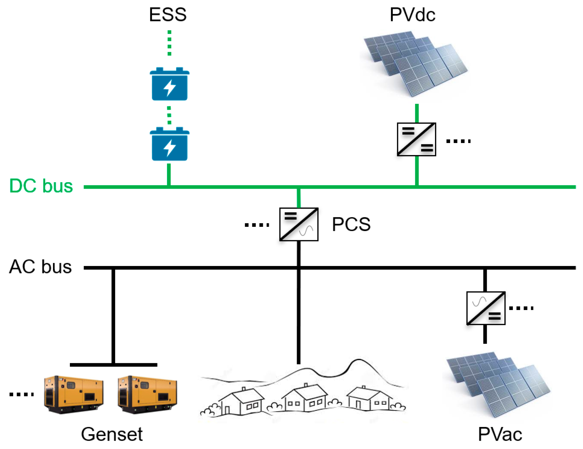
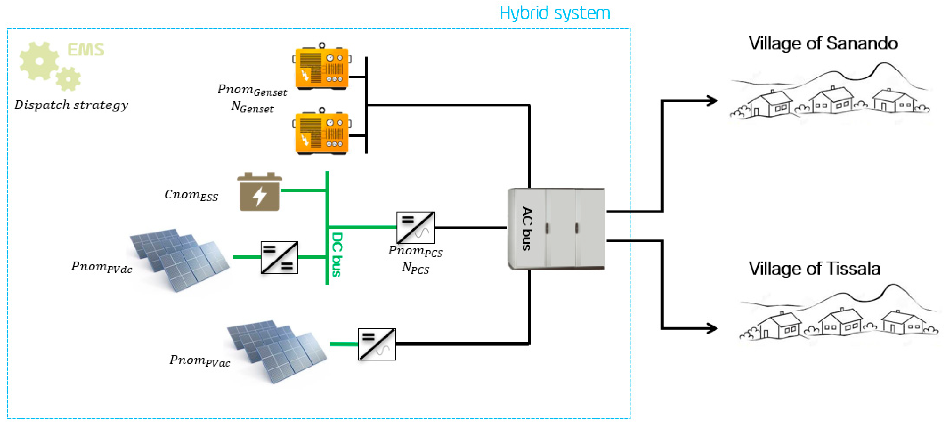
This paper focuses on microgrids that have no ability to connect to the grid and are therefore referred to as autonomous microgrids, also known as mini-grids in the context of rural energy access [6,7,8]. These systems have been used for a long time as a solution to bring access to electricity to remote locations where grid extension is unaffordable. The cut in renewable energy prices has introduced new types of autonomous microgrids, based on renewable energy resources and energy storage. The power ratings of these systems can range from as little as 50 kVA to a few MVA. Only PV systems and diesel generators (Gensets) are considered as the potential sources of generation. PV arrays can be either DC coupled (PVdc), AC coupled (PVac), or integrated into a hybrid architecture where one part of the solar system is connected to a DC bus and another part is connected to an AC bus. Figure 1 shows the microgrid architecture that is considered for the paper. Energy storage systems (ESSs) are used to store excess renewable energy, allowing for a further decrease in the use of fossil-based generation and can be in the form of electrochemical, kinetic, compressed air, or gravitational; however, only battery storage is considered in this paper. A power conversion system (PCS) is required to interface the DC sources (ESS and PVdc) to the AC bus.
Several articles have reviewed the methodologies proposed for the sizing and optimization of autonomous hybrid systems [9,10,11,12,13,14]. Al-falahi et al. [10] listed various indicators used as design objectives. Most of them are economic, reliability, and environmental indicators. Social indicators can also be found in some papers. The authors have observed that single-objective articles were focusing on the optimization of a cost indicator, whereas multi-objective articles were often focusing on the objectives of cost and reliability. The cost thus represents the first optimization objective and includes investment, operation, maintenance, and replacement costs. A recent review on the sizing methodologies of hybrid renewable energy systems from Lian et al. [15] shows that a large proportion of the reviewed sizing methodologies were focusing on off-grid/autonomous applications (79%). To classify the different methods available, Tezer et al. [11] distinguish classical optimization approaches to meta-heuristic approaches. Classical methods require limiting mathematical properties linked to the objective function and include for example the iterative optimization method and linear programming. Meta-heuristic methods include higher-level algorithms to control the whole process of search to explore the solution space efficiently and avoid local optima. These methods can be applied to a wide range of optimization problems. We can distinguish “neighborhood” meta-heuristics developing a single solution at a time to “distributed” or “population-based” meta-heuristics that process a whole population at a time, such as particle swarm optimization (PSO) and genetic algorithms (GA). Various articles have used genetic algorithms to size hybrid energy systems. Katsigiannis et al. [16] use the NSGA-II to design a small autonomous hybrid power system comprising of both renewable and conventional power sources with the objectives of minimizing the energy cost of the system and total greenhouse gas emission during the system lifetime. Reliability was however not considered. Kamjoo et al. [17] have used the NSGA-II algorithm to obtain the trade-offs between cost and reliability in order to size a wind/solar/battery system. Roy et al. [18] used the NSGA-II algorithm to size a multi-energy system solely on renewable energy under the objectives of cost (LCOE) and reliability. Refs. [19,20,21,22,23] have considered long-term sizing with multi-step investments using optimization techniques.
Some reviews also focus on available tools for the design and planning of hybrid renewable energy systems [24,25,26]. Various articles use the software Homer to size hybrid energy systems [27]. Homer is an optimization software that is used to design hybrid systems for microgrid/stand-alone applications. It performs simulations of all possible configurations, calculates energy flows, and lists results according to their relative cost of energy (COE). iHOGA is another hybrid system optimization tool that can be used similarly to model and simulate various components [28]. The authors in [29] make a comparative assessment of Homer and iHoga using a case study, with the motivation that the latter has not been explored as much in the literature. An interesting feature of iHOGA is its ability to perform multi-objective optimization, using up to three objectives (Net Present Cost, CO2 emissions, and Unmet Load), it offers also more flexibility in the control strategies used in the simulations.
Reliability can have different meanings and can account for different aspects depending on the application and field. It can be summarized as the ability of a system to perform as intended without any failure and within the desired performance limits for a specified time, in its lifetime conditions [30]. In power systems, reliability deals with power interruptions, whereas power quality concerns the quality of the sine wave when power is available. Therefore, phenomena of interest in power quality studies, such as swells, swags, impulses, and harmonics are not explored in reliability studies. The reliability of power systems can be separated into adequacy and security [31]. Adequacy relates to the ability of power systems to supply the demand with adequate generation and transmission facilities with a desired level of reserve and can be evaluated in long-term planning studies [30]. Security relates to the ability of the power system to withstand sudden contingencies and outages and is more often integrated into short-term reliability assessment.
Reviews have investigated the use of reliability objectives in designing hybrid systems. Several studies involve reliability assessment in the design of microgrids [32,33,34,35,36]. Most of the reliability indicators used relate to adequacy assessment and account for the risk that generation is lower than consumption [11]. The main adequacy indicators used in the literature for sizing hybrid systems are loss of power supply probability (LPSP), loss of load probability (LOLP), expected energy not supplied (EENS), deficiency of power supply probability (DPSP), loss of load expected (LOLE), and loss of energy expected (LOEE) [15]. The software tools for hybrid system optimization mentioned above also account solely for system adequacy. In the Homer software, reliability can be used as a constraint, specifying a maximum capacity shortage fraction allowed. This capacity shortage accounts for the shortage of generation to power the load, as well as insufficient reserves from the reserve requirement set up by the user. iHOGA also includes a reliability constraint using the indicator of unmet load; however, this indicator does not account for operating reserves.
Some papers in the literature have investigated the security assessment of microgrids. In [37], Paliwal et al. use a Particle Swarm Optimization method to determine optimal autonomous microgrid component sizing with the incorporation of reliability constraints. The reliability analysis of the microgrid is carried out using a multi-state availability model (MSAM) of different generators to calculate the percentage of risk state probability (generation is inadequate to supply load) and the percentage of healthy state probability (system has adequate reserves). Xu et al. [38,39,40] have integrated the consideration of protection and operation into the reliability evaluation of microgrids. However, the reliability analysis developed is not focusing on purely autonomous microgrids with centralized generation and is not integrated into a design method. Escalera et al. [41] suggest that security aspects could be incorporated into reliability analysis in the design phases of microgrids, as the size of the considered systems is small enough to limit the computation time. Security assessment, which in conventional power systems is performed with a short-term horizon, could thus be implemented in long-term planning. Peyghami et al. [30] introduce a new framework for the reliability evaluation of modern power systems. According to the author, security assessment would focus on static phenomena, dynamic and transient, and cybersecurity. In rural autonomous microgrids, security issues are mainly concerned with the stability and thermal limitations of the power electronic interfaces. These limitations impact considerably the protection scheme of the microgrids, as those are typically based on conventional overcurrent devices.
There is thus a research gap in the literature related to the consideration of reliability in the design of isolated microgrid systems, often focusing solely on adequacy. There is a need to model how the design can influence reliability, considering other aspects, such as component failure and protection. There is also a need to explore further the trade-off between design objectives such as cost, reliability, and renewable integration. Therefore, this paper proposes a novel method to size individual components as well as redundancy by exploring the trade-offs between the objectives mentioned above and considering the impact of component failure and protection malfunction on reliability. It aims not to return the optimal sizing of the system, but rather to give the designer the means to carefully select the preferred option according to the observed trade-offs. The method is described in Section 3. A case study is presented in Section 4, and the results obtained from applying the method to this case study are discussed in Section 5 before a conclusion is drawn.
3. Method for Sizing Autonomous Microgrids
This section describes the methodology developed for the sizing and design of autonomous microgrids. The methodology aims to give the user the means to select the optimal component sizing, architecture, as well as control strategy, regarding the objectives of cost, renewable integration, and reliability. There are two general approaches to solve multi-objective optimization problems. The first approach consists of collecting all objectives into a single objective function, using a weighted sum, or treating some objectives as constraints [11]. The second approach is Pareto-based optimization, which uses the Pareto-dominance concept. The Pareto-front is the set of all solutions for which the corresponding objective vectors cannot be improved in any dimension without degradation in another [20]. When considering three objectives, the Pareto-front becomes a three-dimensional surface. The Pareto-based approach was preferred because it does not require fixing a priority or a limit on one of the objectives and it gives the ability to observe trade-offs between optimization objectives.
3.1. Global Multi-Objective Optimisation Method
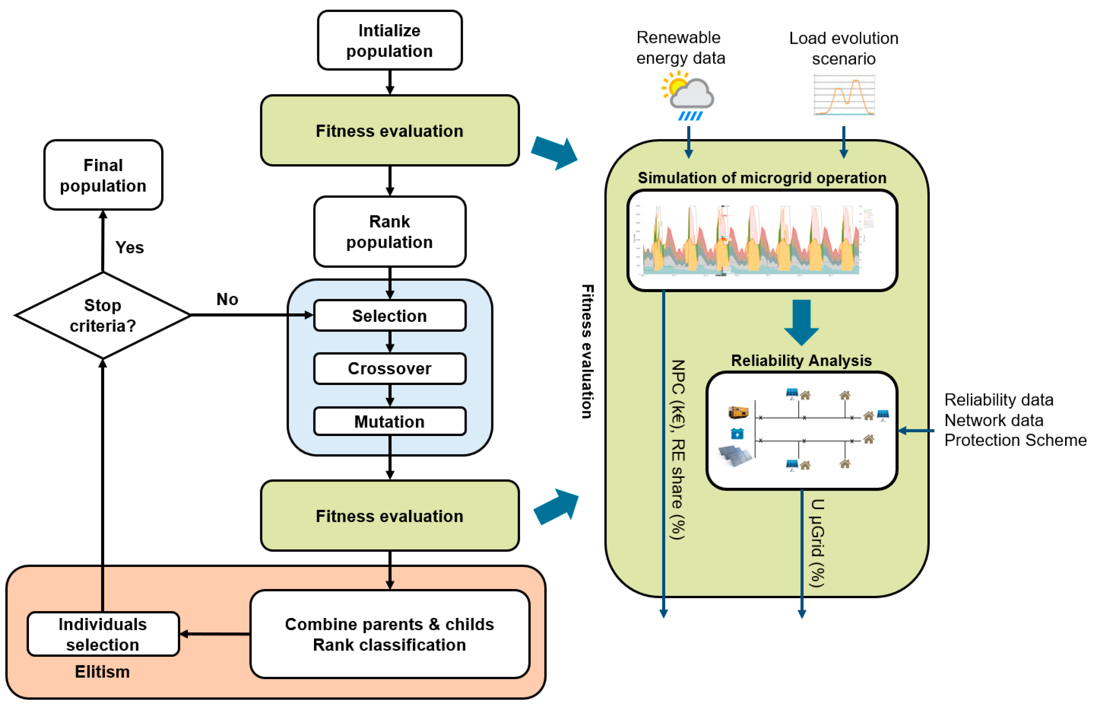
A genetic algorithm was selected for its ability to implement various control algorithms and component models without the need to adapt the optimization formulation. A schematic of the global method developed is presented in Figure 2. This method is presented in [42]. In the evaluation of each microgrid configuration, the simulation gives indicators for the objectives of cost and renewable energy integration and the reliability analysis gives the indicator of unavailability. Both evaluations are performed in a python environment [43]. The planning horizon is 15 years.
The genetic algorithm NSGA-II, developed by K. Deb et al. [44], is used to obtain the non-dominant pareto frontier of the objectives. The advantage of this type of algorithm is that it can efficiently explore the search space. It starts with creating an initial population of a predefined size. Each individual from the population is then evaluated with the simulation and reliability analysis. The population is then ranked based on three indicators (cost, renewable integration, reliability). The algorithm applies a selection, crossover, and mutation to create a new child population. The parent population and children are then combined and ranked to select individuals for the new generation. This process is replicated until the stop criteria are reached. The selection is based on elitism, ensuring the non-dominated individuals from the combined parent and child populations are passed to the next generation.
The variables to optimize are shown in Table 1. Redundancy of diesel generators and PCS inverters is also considered. Different dispatch strategies are considered including “load following” and “cycle charging” as defined in [45]. The NSGA-II algorithm is implemented with the package Pymoo [46], whose settings are given in Table 2. The computation requirement for a population size of 65 is around 11 min per generation.
The first optimization objective is the net present cost (NPC) expressed in k€, and is calculated through Equation (1), where is the net present cost of component i and includes investment cost , yearly operation cost , and replacement cost , as calculated in Equation (2). is the discount rate.
The second optimization objective is the renewable integration as is calculated with Equation (3). The objective is calculated through Equation (3), with being the power produced by all gensets at time t, being the load consumption at time t, being the simulation time step, and T the total number of time steps in the project duration considered.
The third optimization objective concerns reliability. The unavailability is to be minimized and is given as the ratio of the expected energy not served (EENS) to the yearly load demand. The EENS indicator is a sum of three components which are detailed in Section 3.3.
3.2. Simulation Platform Developed
The simulation is made in Python 3.6 (Python Software Foundation, https://www.python.org/ (accessed on 22 July 2021)) and is based on various models describing the behavior of the different microgrid components [43]. The simulation time step is taken as 10 min to account for variability in the load and renewable energy production as well as to model the control of microgrid components with sufficient time resolution. The input data is available as 1-year irradiation and temperature data as well as 15-years load consumption data. Only active power flows are considered in the simulation. The same model is used to calculate the power at the Maximum Power Point for the PV array connected to the AC bus () and the one connected to the DC bus (). Equation (5) describes the model where is the nominal power of the installed PV array (kWp), is the global horizontal irradiance in the plane of array (W/m2), and is the efficiency of the global PV array.
(p.u.) includes temperature losses, inverter losses, and other miscellaneous losses as calculated in Equation (6), where is the inverter efficiency at time t (p.u.), are constant losses and account for cable losses, mismatch, and dirt (p.u.), is the temperature derating coefficient according to the datasheet of the PV module (%/°C), is the module cell temperature (°C), and is the reference cell temperature at Standard Test Conditions (°C).
The module cell temperature is calculated as per Equation (7), where is the ambient temperature at time t (°C), is the nominal operating cell temperature [°C], is the nominal operating ambient temperature (°C), is the nominal operating irradiance (W/m2).
The EMS model calculates active power setpoints for each microgrid component. Only the battery system does not receive a setpoint as its power output is the difference between the power from the bi-directional inverter and the power produced by the PV array connected to the DC bus, both controlled by the energy management system (EMS).
The genset controller model decides to start/stop individual gensets and dispatches the global genset power setpoint to each available unit. The PV converter model applies a saturation of the active power setpoint to the nominal power rating of the converter as well as an efficiency based on an efficiency versus operating power curve. The PCS also applies a saturation and an efficiency to the setpoint but allows for bi-directional power flow.
3.3. Reliability Analysis Method
As discussed in Section 2, reliability can address both adequacy and security aspects. In the sizing method developed, security aspects of component failure and protection failure are considered in addition to generation adequacy. These two aspects considered are described in this section. The system size is sufficiently small to be able to integrate these aspects in a genetic algorithm with acceptable computation time. The methodology is described in this section.
3.3.1. Adequacy Assessment
Adequacy relates to the ability of power systems to supply the demand with adequate generation and transmission facilities with a desired level of reserve and can be evaluated in long-term planning studies [30]. The indicator used in this paper for assessing adequacy is the expected energy not supplied (EENS), which can be calculated from the simulation results. At each time-step, the load power not supplied due to insufficient generation capability is obtained from Equation (8), being the sum of active powers from all generating sources. The EENS indicator is then calculated from Equation (9).
3.3.2. Contingency Enumeration Method
The first security aspect considered is the static response to component failure. Different methods exist to obtain reliability indices in this regard. An enumerative contingency analysis, often used for reliability analysis on conventional power systems, can be easily applied for this application as a small number of components are present in the type of microgrids considered. The following component failures are considered:
- Failure of an AC-coupled PV array;
- Failure of a DC-coupled PV array;
- Failure of a diesel generator;
- Failure of the battery system;
- Failure of a PCS inverter.
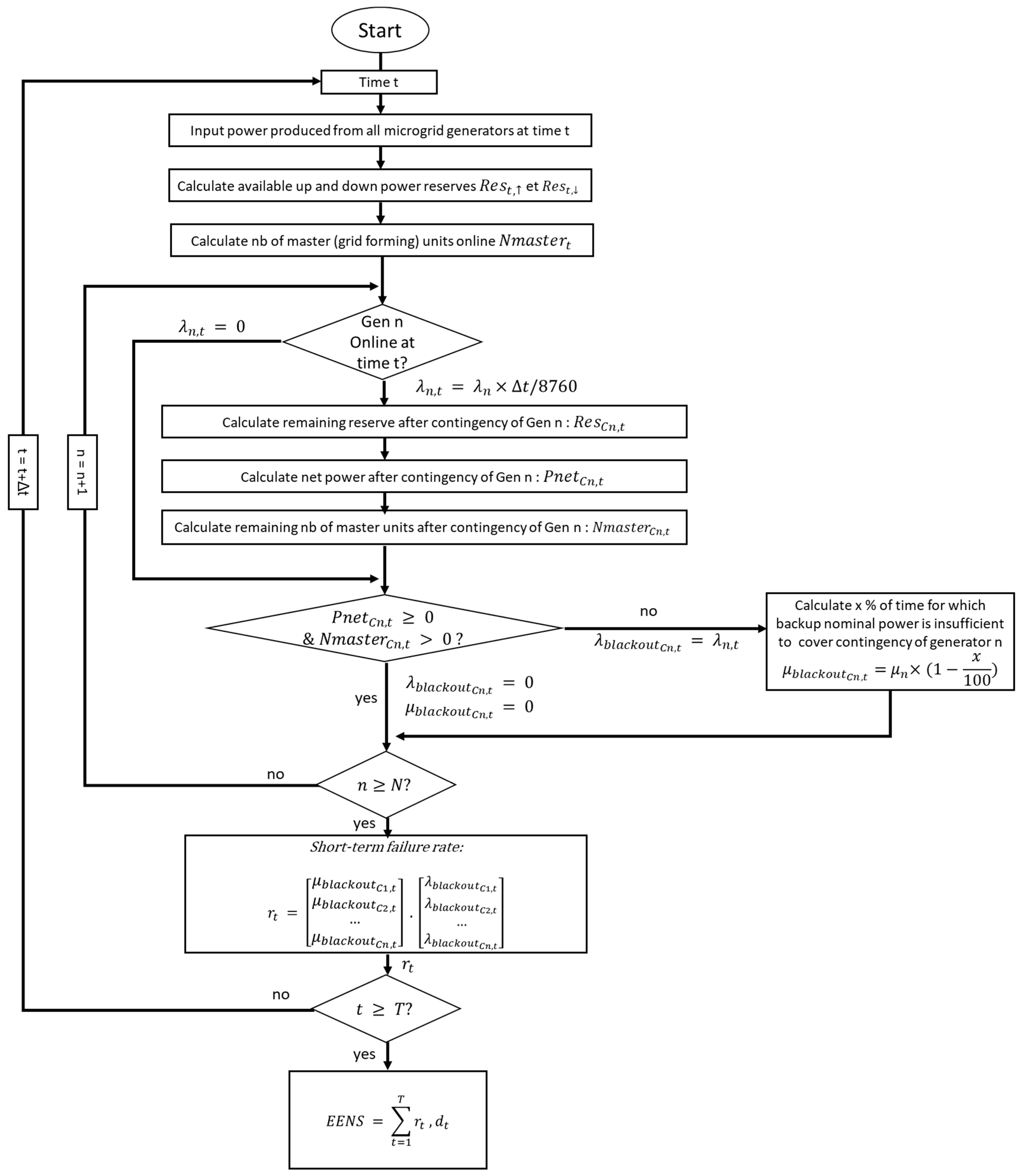
Each component is modeled with a short-term failure rate corresponding to the failure probability of component n at time step t. Failure rates are assumed constant throughout the component life. A blackout state is obtained when there is not enough reserve power to counteract the contingency or when no backup master unit is available to take over the role of grid-forming. For each of the considered failures, the steps illustrated in Figure 3 are followed.
First, the available up and down reserves before contingency are calculated for each time step from the simulation results. The reserve of the storage system and the reserve of the diesel generators are assumed to be effective in counterbalancing generator failures and to be independent of the grid-forming configuration. The storage system reserve (up and down) is the minimum between the power reserve available on the inverters and the power reserve available in the batteries that could be released during the time required to turn on/off an additional generator (if available). The reserve on the diesel generators is calculated based on their nominal power rating for the up-regulating reserve and based on their minimum acceptable operating power for the down-regulating reserve. The number of master units (operated in grid-forming) depends on the selected grid-forming configuration. In this paper, we consider a single-master configuration, where the grid-forming unit(s) is switched between a diesel generator(s) and the PCS inverter(s).
For each considered contingency, the available up and down reserves after the failure of element n, , are calculated by subtracting the reserve provided by the failed unit from the available reserve before contingency. The net power after contingency is then calculated by subtracting the power produced by the failed unit from the available reserve after failure. It is used to estimate whether the available reserve at time t is sufficient to counterbalance the loss of element n. If at t, component n is generating power, then the up-regulating reserve is used. However, if it is absorbing power, the down-regulating reserve is used. The loss of element n at time t induces a blackout of the microgrid if one of the following conditions are met:
- The net power after contingency is negative: ;
- The number of remaining master units after contingency is zero: .
If a blackout state is predicted, then the blackout rate due to contingency n is equal to the short-term failure rate of element n and a repair time is allocated. This repair time depends on the remaining nominal power available in the microgrid after contingency. If sufficient nominal power is available to power the load, the repair time is only the time taken to restart the microgrid. Otherwise, the repair time is calculated according to the time the microgrid can be maintained online with the remaining nominal power. The short-term reliability index at each time step t is calculated by summing each product of failure rate and repair time corresponding to all considered contingencies:
The chosen index to evaluate the reliability related to component failures is the expected energy not supplied (EENS) and is calculated with Equation (11).
3.3.3. Protection Reliability Assessment
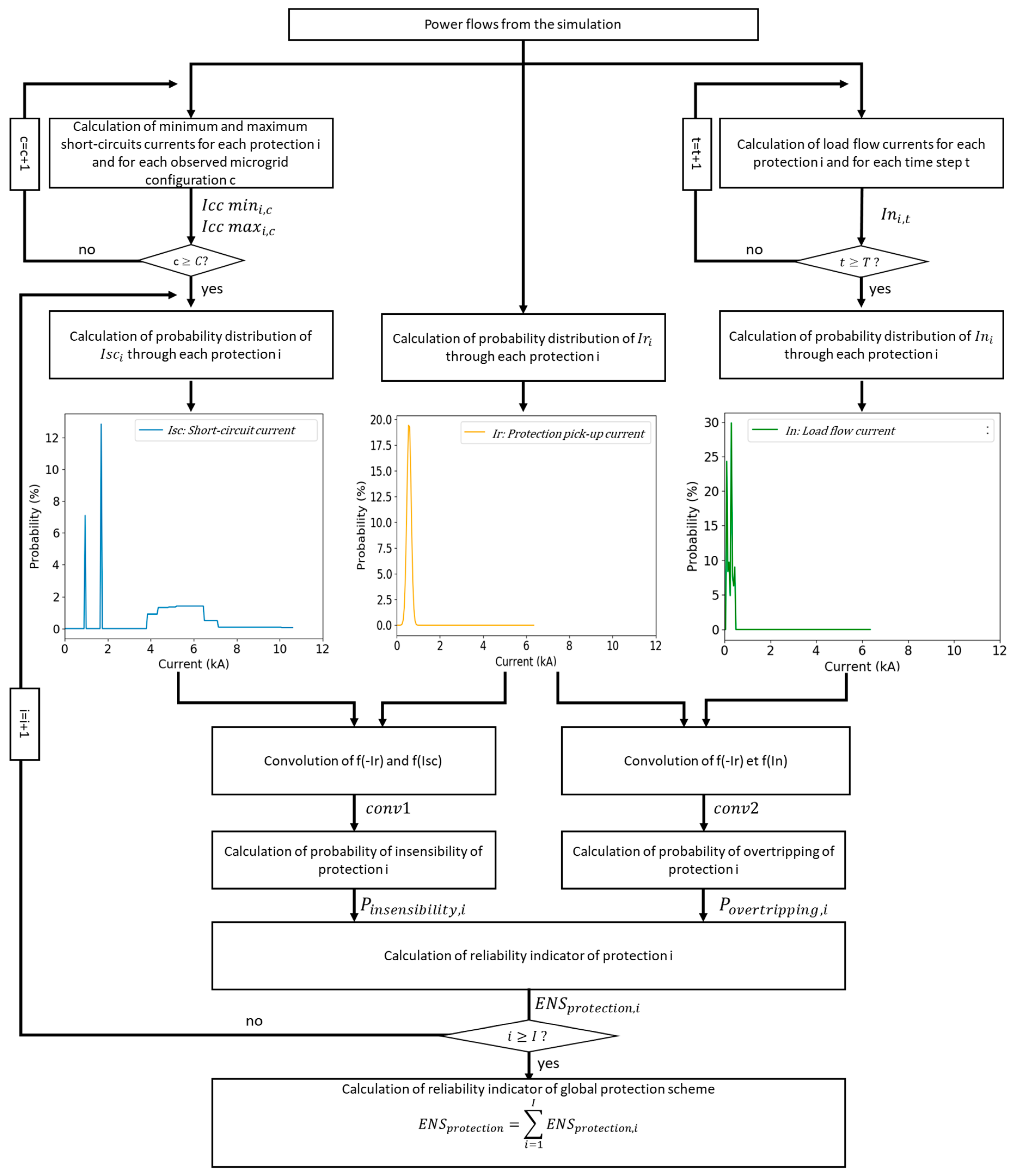
Protection selectivity is another important issue to address in autonomous microgrids, especially as the microgrids of interest can operate in various modes with different short-circuit levels available. There is a need to design a protection scheme that is operating well in all configurations of the microgrid. The protection scheme that is used in our case is based on conventional overcurrent relays and fuses. These devices require a sufficient level of short-circuit current to operate in case of a fault.
Reliability analysis of the protection scheme aims at assessing how well the protection will perform for a particular architecture and sizing, regarding coordination and selectivity, considering two possible causes of protection malfunction:
- The insensitivity of protections in the case of insufficient short-circuit contribution to trigger the right protection;
- Overtripping in the case of protection triggering in healthy operation of the microgrid.
The different steps toward the protection reliability assessment method are described in Figure 4. The microgrid is modeled with the package Pandapower [47] in the Python environment, which is used for static network analysis. All buses, lines, converters, and loads are modeled. The first step consists of calculating short-circuit currents on each microgrid configuration observed from the simulation. These configurations correspond to all possible on/off combinations of the different short-circuit current contributors, including gensets, PCS inverters, and PVac inverters. Next, load flow simulations are made for each simulation time-step to calculate the current flowing through each protection. Reliability indicators are then calculated to assess the protection scheme. Three probability distributions must be obtained to calculate these reliability indicators:
- The probability distribution of short-circuit current in each protection Isc (blue line in Figure 4). This distribution is obtained using the minimum and maximum short-circuit current calculated for each microgrid configuration and the frequency of occurrence of each configuration;
- The probability distribution of the load flow current In (red line in Figure 4). This distribution is obtained directly from the load flow calculation made for each simulation time step;
- The probability distribution of the pick-up current Ir (orange line in Figure 4). This distribution is modeled with a normal distribution with a mean equal to the pick-up setting.
The probability of insensitivity of protection i is the probability that the pick-up current is higher than the short-circuit current available at the protection. This probability is calculated by Equation (12) using a convolution of the probability distributions of Ir and Isc:
The probability of the over-tripping of protection i is the probability that the load flow current In is higher than the pick-up current Ir. This is illustrated in Equation (13) and also calculated by convolution:
These indicators are then combined into a single indicator for reliability assessment of the protection scheme, which is the expected energy not supplied (EENS), calculated with Equations (14)–(17), being the short-circuit rate, the mean power flowing through protection i (obtained from simulation results), the short-term repair time of faults, and the repair time following a blackout.
4. Case Study Description
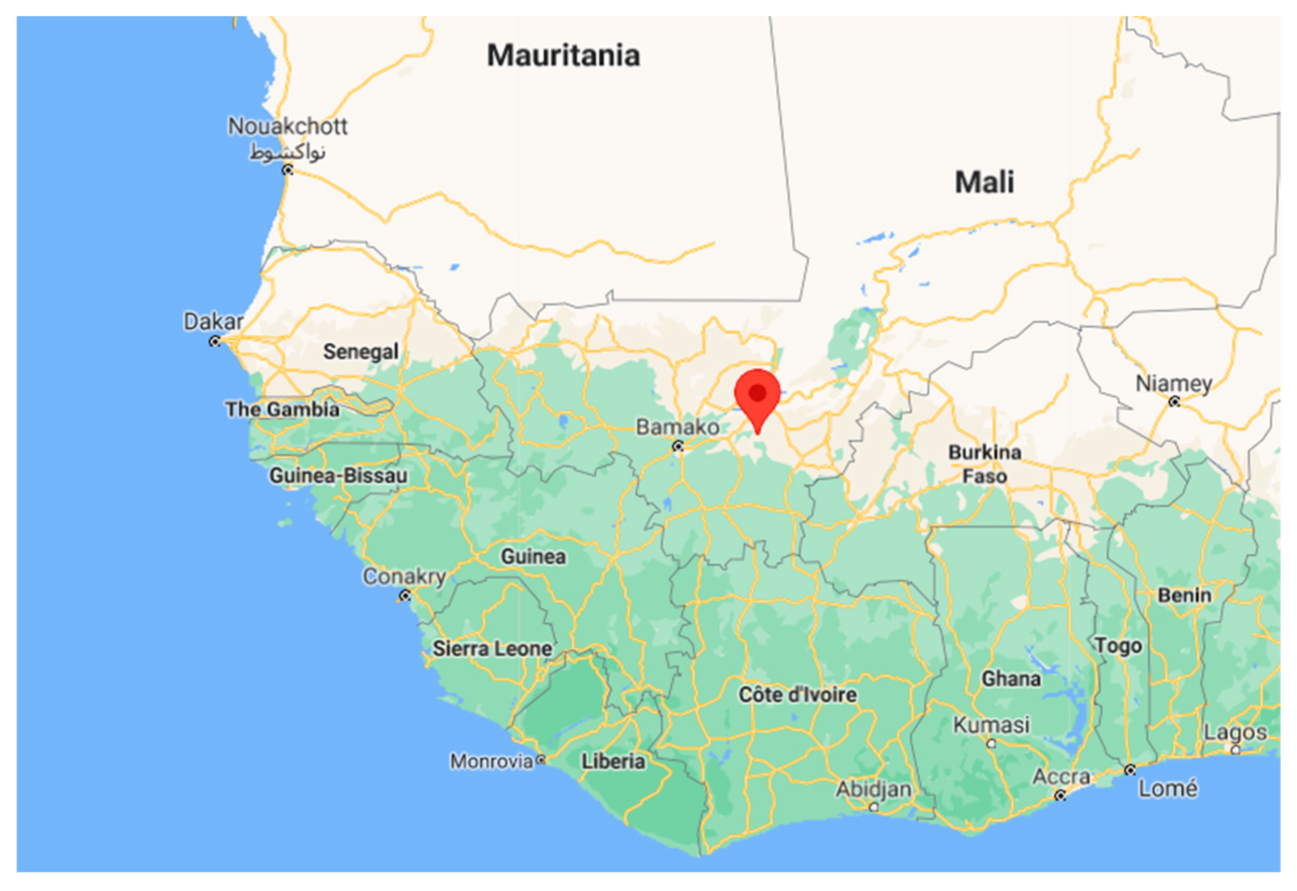
The methodology introduced in the previous section was applied to a case study of an autonomous microgrid currently in installation in the rural localities of Sanando and Tissala in Mali, shown on a map in Figure 5. This microgrid project was enabled by the Energizing Development Program (EnDev) and coordinated by GIZ together with AMADER and the municipality of Sanando. This project aims to build a hybrid power station including a solar PV array, a diesel generator (Genset), and a battery storage system (ESS + PCS) connecting both villages. The operation and maintenance of the microgrid will then be carried out by a consortium including Entech Smart Energies and Sinergie SA. There was initially no electricity grid available to inhabitants, some of them relying on individual solutions (gensets or small solar systems).
The objectives of the operation of the hybrid system to be installed in the villages of Sanando-Tissala are to minimize fuel consumption on-site, to limit the aging of the equipment, and minimize the risk of blackout. To optimize the performance of the system, the following functions will be implemented in the Energy Management System:
- Energy shifting—this function allows excess solar energy to be stored during the day for later redistribution.
- Genset off capability—this function enables the microgrid to operate on solar + storage only without any diesel generator online. It requires the grid-forming capability on the PCS inverters to be able to stabilize frequency and voltage.
- Spinning reserve—this function enables the monitoring of available reserves on the different generators and control the PCS inverters to ensure a certain level of reserve (both upregulation and downregulation).
Figure 6 shows the layout of the case study with the variables to optimize using the method. A wide range of values were considered for the optimization variables as shown in Table 3.
The simulation of the system operation requires various technical parameters whose values are shown in Table A1 in Appendix A. To calculate the net present cost of each sizing configuration, cost parameters regarding investment, operation, and replacement are also required for each component and are shown in Table A2. Investment costs are modeled with two coefficients, as proposed in [48]. Coefficient b accounts for the decreasing unit cost of the equipment with increasing size. The resulting investment cost is given by Equation (18).
The reliability parameters are given in Appendix A in Table A3 for the contingency enumeration method and in Table A4 for the protection reliability assessment.
5. Results and Discussion
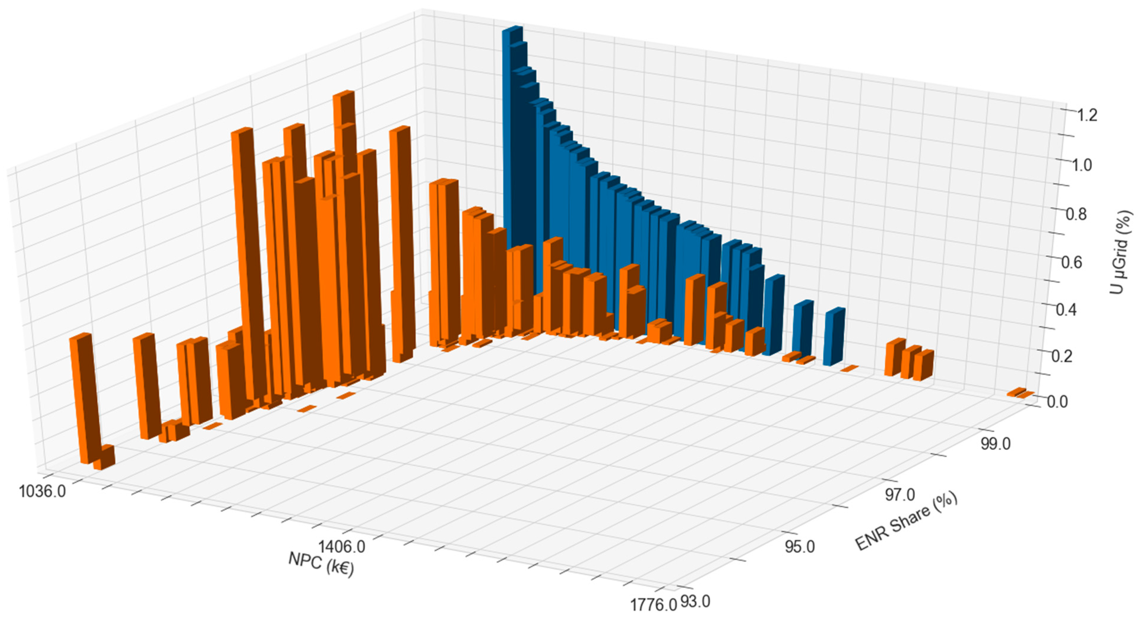
The multi-objectives optimization method presented in Section 3 was applied to the case study. The NSGA-II has led to the 3D Pareto surface shown in Figure 7. There is a strong relationship between all three objectives. To increase the renewable energy integration, an increase in net present cost is required. Configurations without gensets (in blue) lead to an increased unavailability and increased net present cost compared to configurations with gensets (in orange). Configurations with renewable energy integration less than 93% are not included in the Pareto frontier. They are thus not leading to an improvement in either net present cost or reliability. Considering the control strategy, only load following dispatch was found in the Pareto surface, which proves this type of control more interesting for this level of renewable integration.
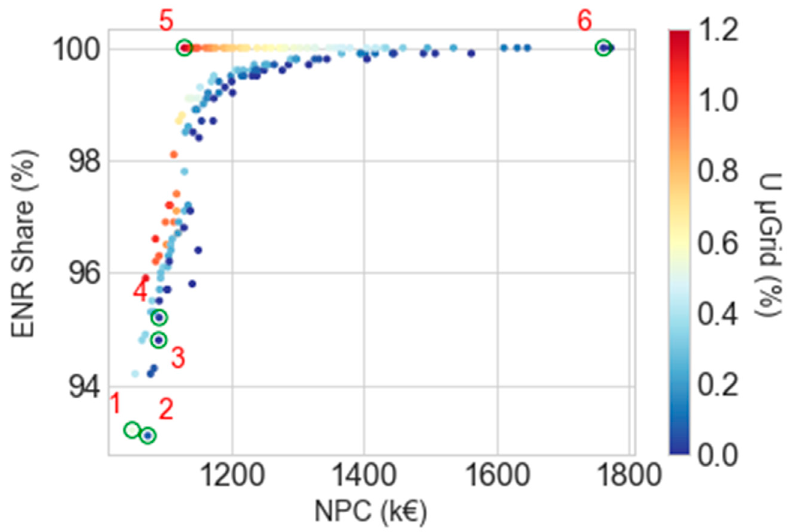
Figure 8 shows the same Pareto points in a 2D graph with the third objective of reliability shown in a color scale. It can be observed that reliability can be improved with a small increase in net present cost for a similar renewable energy integration. In this figure, six configurations of interest have been selected for more detailed analysis:
- Least cost: the configuration with the least net present cost;
- Cost/reliability trade-off: the configuration with the least net present cost that has an unavailability less than 0.1%;
- Most reliable: the configuration with the lowest unavailability;
- Cost/reliability/RE trade-off: the configuration with the least net present cost that has an unavailability less than 0.1% and a renewable energy integration above 95%;
- Most renewable: the cheapest configuration with 100% renewable energy integration;
- Reliability/RE trade-off: The configuration with the highest renewable integration and unavailability less than 0.1%.
The least-cost configuration (config 1) can be obtained at a net present cost of 1.050 M€ over the 15-year period considered. An improvement in reliability (config 2) can be obtained for a net present cost of 1.074 M€. A solution with 0% unavailability (config 3) can be obtained at a cost of 1.089 M€. A compromise between all three objectives (config 4) can be found for a net present cost of 1.091 M€, having a renewable energy integration above 95% and an unavailability under 0.1%. A 100% renewable energy solution can be obtained for a net present cost of 1.130 M€ but with high unavailability of 1.2% (config 5). Reaching a high level of reliability with 100% renewable energy integration (config 6) would require oversizing considerably the components and, therefore, adds significant costs to the design (1.76 M€).
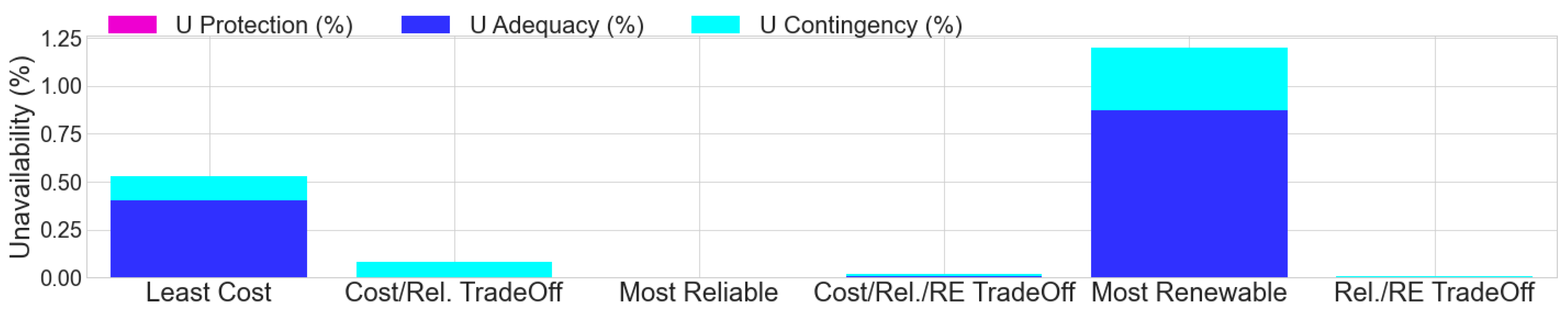
These six configurations are further explored in the following figures. In Figure 9, the reliability indicator is decomposed into the different aspects considered. The least-cost configuration has a significant lack of generation capacity ( of 0.4%). The most renewable configuration also has a significant unavailability related to adequacy and to contingencies. For other configurations, unavailability is essentially related to contingencies. The aspect of protection is well managed in these six configurations with a sufficient short-circuit capacity and the configurations of the Pareto surface have an unavailability related to protection malfunction that is null.
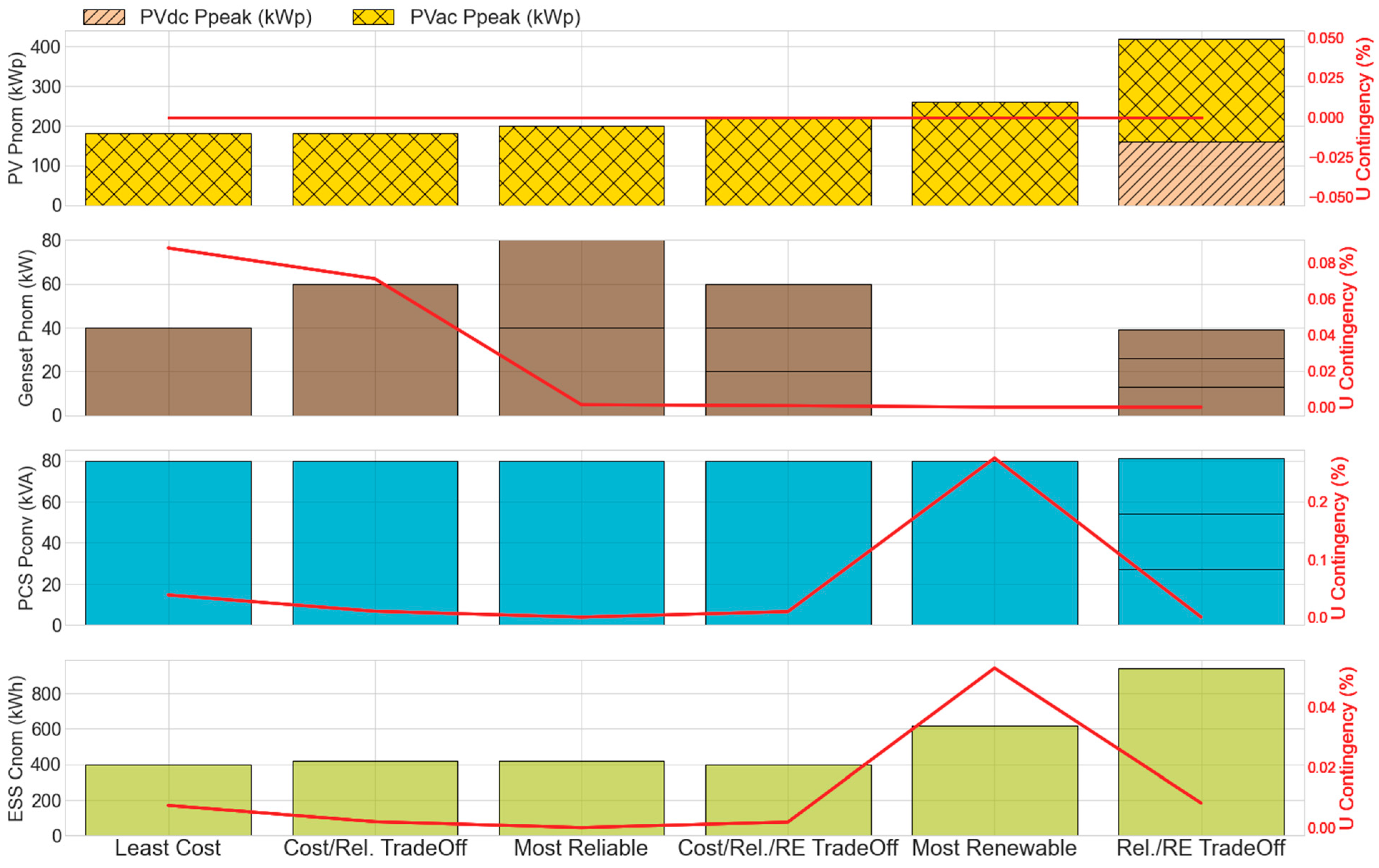
Figure 10 shows the installed PV power, battery capacity, PCS power, and the genset nominal power. In terms of architecture, AC-coupled PV power was preferred, except for the reliability/RE trade-off which is a hybrid AC/DC configuration. The least-cost configuration has a small renewable energy capacity in terms of PV power and battery capacity installed (180 kWp/400 kWh). To increase the reliability (cost/reliability trade-off), an increase in the genset capacity is required (60 kW). The most reliable configuration is similar to the “cost/reliability trade-off” with an increase in PV power (200 kWp) and an additional genset unit (2 × 40 kW). The fourth configuration, being a compromise on the three objectives, requires a small increase in PV power and battery capacity as compared to the least cost option as well as three genset units installed (3 × 20 kW). The most renewable configuration has a significant amount of PV power installed (260 kWp) and ESS (620 kWh). The configuration with the most renewable integration and constrained unavailability (reliability/RE trade-off) leads to a further increase in PV and battery capacity, without reaching 100% renewable integration. This configuration has also three 13 kW gensets installed, as well as three PCS units of 27 kVA each. Apart from this configuration, an optimum size of one unit of 80 kVA for the PCS inverter is found.
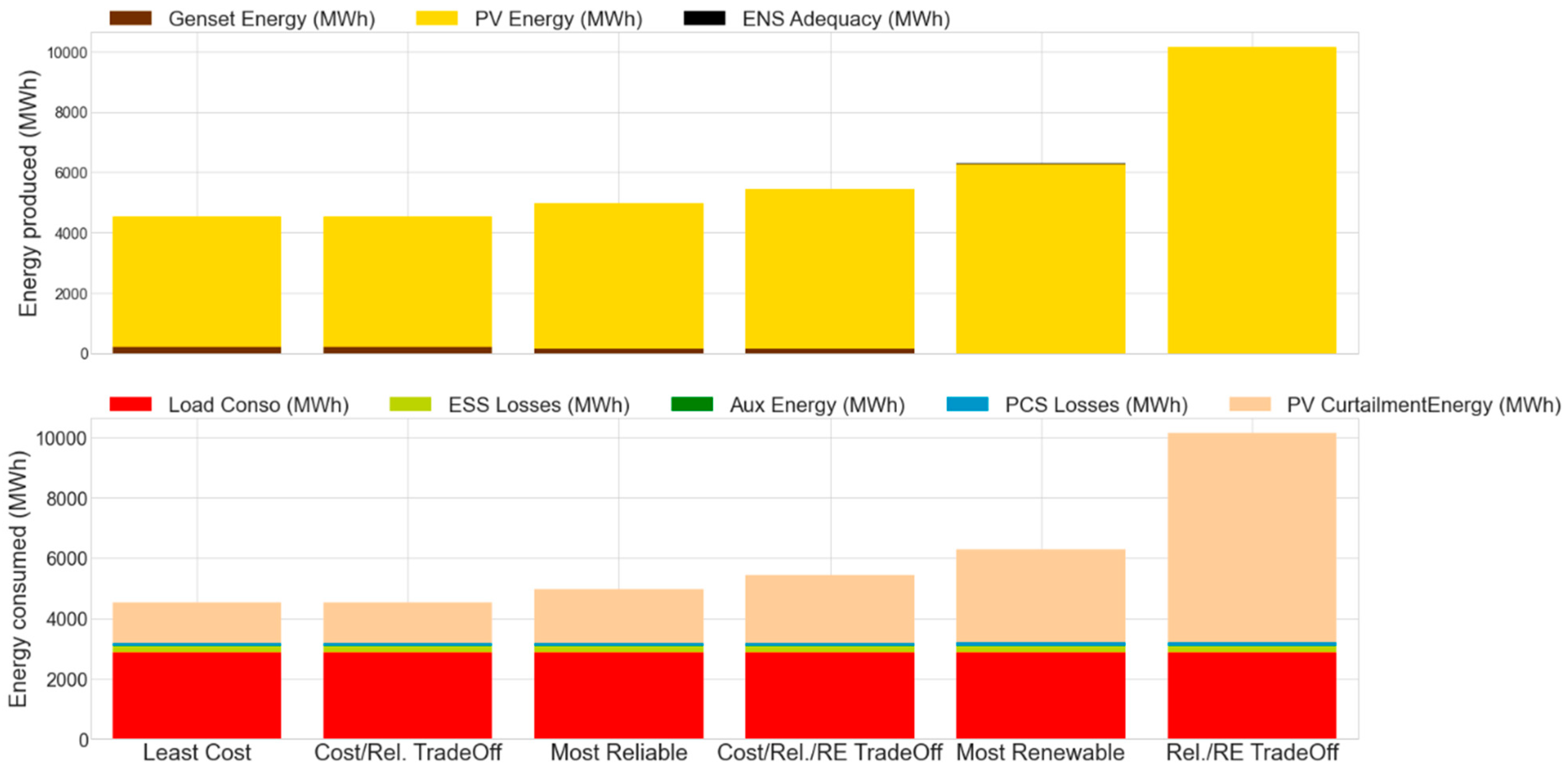
Figure 11 shows the energy flows in the 15-year period for each of the six selected configurations. A small part of the energy production in all configurations is from the gensets. When looking at how this energy is consumed, an important share of the PV production is curtailed, from 31% for the least cost configuration up to 68% for the reliability/RE trade-off.
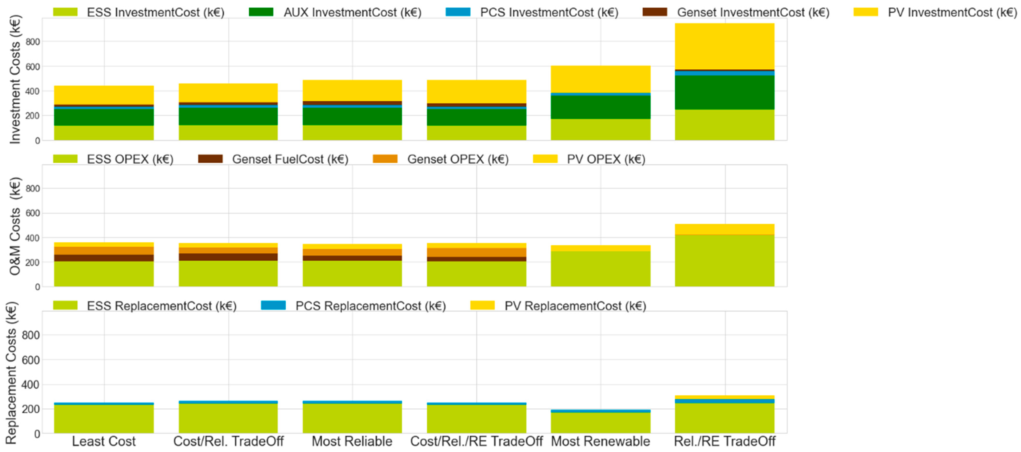
Figure 12 shows the cash flows involved in these six configurations. The investment costs are dominated by the ESS and PV systems. BOS corresponds to the balance of system costs to integrate the storage system. Regarding O&M costs, fuel and genset maintenance costs are a significant part of the two first configurations but are less dominant as renewable integration is increased. The replacement costs are dominated by battery costs. Although, the “most renewable” and “reliability/RE trade-off” configurations have a larger battery capacity installed, the cycling is expected to be less and, therefore, the battery replacement cost over the 15 years is less important.
6. Conclusions
This paper presents a method to optimize an autonomous microgrid considering the three design objectives of cost, renewable integration, and reliability. The multi-objective optimization is implemented with a genetic algorithm and involves a simulation of the system operation as well as a reliability analysis for each configuration evaluated. By accounting for reliability related to component failure and protection, the method gives an additional investigation on the impact of microgrid design on power availability. Additionally, rather than finding a single optimal configuration, it helps to understand the trade-offs between all objectives and estimating the cost of improving either renewable integration, reliability, or both. This method was applied to a case study of a rural microgrid in Mali to size the different microgrid components. The Pareto surface obtained shows all non-dominated solutions over the three design objectives. It was first observed that high renewable integration could be obtained without impacting the long-term cost and reliability. The cost of having high reliability was found to be low in this typical case study. Six different solutions were illustrated, each representing a trade-off between the three design objectives. With the proposed method, the user can decide to select a sizing according to the chosen trade-off. Reaching a high level of reliability with 100% renewable energy integration would require oversizing considerably the components and, therefore, add significant costs to the design. Moreover, it leads to an important curtailment of surplus renewable energy. This energy could however be used for other applications such as long-term energy storage, water heating, or water pumping.
Author Contributions
Writing and editing, M.R.; supervision, F.D.-R., D.G., C.L.L., Q.T.T. and M.B. All authors have read and agreed to the published version of the manuscript.
Funding
This research was supported by ANRT.
Data Availability Statement
Not applicable.
Acknowledgments
The authors would like to thank the GIZ for its contribution to this paper and for giving us the opportunity to apply our method to a real case study.
Conflicts of Interest
The authors declare no conflict of interest.
Appendix A. Parameters of the Optimization Method

Table A1.
Technical parameters of the optimization method.
| Component | Variable | Unit | Value |
|---|---|---|---|
| Genset | % | 30 | |
| % | 120 | ||
| ) | L/kWh | (0.466, 0.304, 0.305, 0.325, 0.375) | |
| h | 15,000 | ||
| % | 90 | ||
| % | 40 | ||
| Pvac | % | 96 | |
| % | 10 | ||
| %/°C | −0.35 | ||
| PVdc | % | 97 | |
| % | 10 | ||
| %/°C | −0.35 | ||
| PCS | ) | % | (0.952, 0.962, 0.97, 0.973, 0.974, 0.975) |
| % | 5 | ||
| Batteries | % | 50 | |
| C-rate | p.u. | 1 | |
| % | 93 | ||
| % | 93 | ||
| Aux | kW | 3 | |
| Air conditioning use | On/Off | Off | |
| EMS | Genset Off fun | On/Off | On |
| Spinning reserve fun | On/Off | On | |
| % | 20 | ||
| % | 100 |
Table A2.
Economical parameters of the optimization method.
| Component | |||||
|---|---|---|---|---|---|
| GE | 1821 €/kW | 0.51 | 5 €/OpHr | - | - |
| PVac | 730 €/kW | 0 | /y | fixed year 15 | |
| PVac conv | 130 €/kW | 0 | /y | fixed year 15 | |
| PVdc | 730 €/kW | 0 | /y | fixed year 15 | |
| PVdc conv | 200 €/kW | 0 | /y | fixed year 10 | |
| PCS | 1816 €/kW | 0.45 | /y | fixed year 10 | |
| ESS | 593 €/kWh | 0.12 | /y | at EOL | |
| BOS | 50% overall ESS cost | 0 | /y | - | - |
Table A3.
Parameters for the contingency enumeration method [49].
Table A3.
Parameters for the contingency enumeration method [49].
| Component Type | Failure Rate (f/Year) | Repair Time (h) |
| Genset | 0.20 | 438 |
| PVac | 0.04 | 480 |
| PVdc | 0.04 | 480 |
| PCS | 0.14 | 168 |
| ESS | 0.03 | 168 |
Table A4.
Parameters for the protection reliability assessment.
| Parameter | Unit | Value |
|---|---|---|
| occ/an | 0.2 | |
| h | 4 | |
| h | 4 | |
| h | 2 | |
| % | 10 |
References
- IEA. World Energy Outlook 2019; IEA: Paris, France, 2019. [Google Scholar]
- Iea, I.; UNSD, W. WHO Tracking SDG 7: The Energy Progress Report; World Bank: Washington, DC, USA, 2021. [Google Scholar]
- Bhatia, M.; Angelou, N. Beyond Connections: Energy Access Redefined; World Bank: Washington, DC, USA, 2015. [Google Scholar]
- Aresti, M.; Barclay, A.; Cherubini, P. RE-Thinking Access to Energy Business Models: Ways to Walk the Water-Energy-Food Nexus Talk in Sub-Saharan Africa; Res4Africa Foundation: Rome, Italy, 2019. [Google Scholar]
- IRENA. Africa 2030: Roadmap for a Renewable Energy Future; IRENA: Abu Dhabi, United Arab Emirates, 2015; p. 72. [Google Scholar]
- Amanda Kahunzire Off-Grid, Mini-Grid and On-Grid Solar PV Solutions in Africa: Opportunities and Challenges. Int. Support Netw. Afr. Dev. ISNAD Afr. 2018. Available online: https://isnad-africa.org/2018/09/30/off-grid-mini-grid-and-on-grid-solar-pv-solutions-in-africa-opportunities-and-challenges-renewable-energy-green-energy-solar-energy-amanda-kahunzire/ (accessed on 20 June 2021).
- Asian Development Bank. Deployment of Hybrid Renewable Energy Systems in Minigrids; Asian Development Bank: Manila, Philippines, 2017. [Google Scholar]
- Bhattacharyya, S.C.; Palit, D. (Eds.) Mini-Grids for Rural Electrification of Developing Countries; Green Energy and Technology; Springer International Publishing: Cham, Switzerland, 2014; ISBN 978-3-319-04815-4. [Google Scholar]
- Siddaiah, R.; Saini, R.P. A Review on Planning, Configurations, Modeling and Optimization Techniques of Hybrid Renewable Energy Systems for off Grid Applications. Renew. Sustain. Energy Rev. 2016, 58, 376–396. [Google Scholar] [CrossRef]
- Al-falahi, M.D.A.; Jayasinghe, S.D.G.; Enshaei, H. A Review on Recent Size Optimization Methodologies for Standalone Solar and Wind Hybrid Renewable Energy System. Energy Convers. Manag. 2017, 143, 252–274. [Google Scholar] [CrossRef]
- Tezer, T.; Yaman, R.; Yaman, G. Evaluation of Approaches Used for Optimization of Stand-Alone Hybrid Renewable Energy Systems. Renew. Sustain. Energy Rev. 2017, 73, 840–853. [Google Scholar] [CrossRef]
- Sinha, S.; Chandel, S.S. Review of Recent Trends in Optimization Techniques for Solar Photovoltaic–Wind Based Hybrid Energy Systems. Renew. Sustain. Energy Rev. 2015, 50, 755–769. [Google Scholar] [CrossRef]
- Rey, J.M.; Vergara, P.P.; Solano, J.; Ordóñez, G. Design and Optimal Sizing of Microgrids. In Microgrids Design and Implementation; Zambroni de Souza, A.C., Castilla, M., Eds.; Springer International Publishing: Cham, Switzerland, 2019; pp. 337–367. ISBN 978-3-319-98686-9. [Google Scholar]
- Bourennani, F.; Rahnamayan, S.; Naterer, G.F. Optimal Design Methods for Hybrid Renewable Energy Systems. Int. J. Green Energy 2015, 12, 148–159. [Google Scholar] [CrossRef]
- Lian, J.; Zhang, Y.; Ma, C.; Yang, Y.; Chaima, E. A Review on Recent Sizing Methodologies of Hybrid Renewable Energy Systems. Energy Convers. Manag. 2019, 199, 112027. [Google Scholar] [CrossRef]
- Katsigiannis, Y.A.; Georgilakis, P.S.; Karapidakis, E.S. Multiobjective Genetic Algorithm Solution to the Optimum Economic and Environmental Performance Problem of Small Autonomous Hybrid Power Systems with Renewables. IET Renew. Power Gener. 2010, 4, 404. [Google Scholar] [CrossRef]
- Kamjoo, A.; Maheri, A.; Dizqah, A.M.; Putrus, G.A. Multi-Objective Design under Uncertainties of Hybrid Renewable Energy System Using NSGA-II and Chance Constrained Programming. Int. J. Electr. Power Energy Syst. 2016, 74, 187–194. [Google Scholar] [CrossRef]
- Roy, A. Optimal Energy Management of a Multi-Source System for a Remote Maritime Area. Ph.D.’s Thesis, Université de Nantes (UNAM), Nantes, France, 2019. [Google Scholar]
- Fioriti, D.; Pintus, S.; Lutzemberger, G.; Poli, D. Economic Multi-Objective Approach to Design off-Grid Microgrids: A Support for Business Decision Making. Renew. Energy 2020, 159, 693–704. [Google Scholar] [CrossRef]
- Fioriti, D.; Poli, D.; Duenas-Martinez, P.; Perez-Arriaga, I. Multi-Year Stochastic Planning of off-Grid Microgrids Subject to Significant Load Growth Uncertainty: Overcoming Single-Year Methodologies. Electr. Power Syst. Res. 2021, 194, 107053. [Google Scholar] [CrossRef]
- Petrelli, M.; Fioriti, D.; Berizzi, A.; Poli, D. Multi-Year Planning of a Rural Microgrid Considering Storage Degradation. IEEE Trans. Power Syst. 2021, 36, 1459–1469. [Google Scholar] [CrossRef]
- Stevanato, N.; Lombardi, F.; Balderrama, S.; Guidicini, G.; Rinaldi, L.; Pavičević, M.; Quoilin, S.; Colombo, E. Long-Term Optimal Sizing of Rural Microgrids: Accounting for Load Evolution through Multi-Step Investment Plan. 2. In Proceedings of the 14th Conference on Sustainable Development of Energy, Water and Environment Systems, Dubrovnik, Croatia, 1–6 October 2019; SDEWES Centre: Dubrovnik, Croatia, 2019. [Google Scholar]
- Pecenak, Z.K.; Stadler, M.; Fahy, K. Efficient Multi-Year Economic Energy Planning in Microgrids. Appl. Energy 2019, 255, 113771. [Google Scholar] [CrossRef]
- Kumar, A.P. Analysis of Hybrid Systems: Software Tools. In Proceedings of the 2016 2nd International Conference on Advances in Electrical, Electronics, Information, Communication and Bio-Informatics (AEEICB), Chennai, India, 27–28 February 2016; pp. 327–330. [Google Scholar]
- Sinha, S.; Chandel, S.S. Review of Software Tools for Hybrid Renewable Energy Systems. Renew. Sustain. Energy Rev. 2014, 32, 192–205. [Google Scholar] [CrossRef]
- Erdinc, O.; Uzunoglu, M. Optimum Design of Hybrid Renewable Energy Systems: Overview of Different Approaches. Renew. Sustain. Energy Rev. 2012, 16, 1412–1425. [Google Scholar] [CrossRef]
- HOMER—Hybrid Renewable and Distributed Generation System Design Software. Available online: https://www.homerenergy.com/ (accessed on 6 April 2020).
- IHOGA—Simulation and Optimization of Stand-Alone and Grid-Connected Hybrid Renewable Systems. Available online: https://ihoga.unizar.es/en/ (accessed on 12 March 2021).
- Saiprasad, N.; Kalam, A.; Zayegh, A. Comparative Study of Optimization of HRES Using HOMER and IHOGA Software; NISCAIR-CSIR: New Delhi, India, 2018; pp. 677–683. [Google Scholar]
- Peyghami, S.; Palensky, P.; Blaabjerg, F. An Overview on the Reliability of Modern Power Electronic Based Power Systems. IEEE Open J. Power Electron. 2020, 1, 34–50. [Google Scholar] [CrossRef] [Green Version]
- Vrana, T.K.; Johansson, E. Overview of Analytical Power System Reliability Assessment Techniques. In Proceedings of the CIGRE Symposion, Recife, Brasil, 3–6 April 2011; p. 14. [Google Scholar]
- Mitra, J.; Singh, C. Optimal Deployment of Distributed Generation Using a Reliability Criterion. IEEE Trans. Ind. Appl. 2016, 52, 1989–1997. [Google Scholar] [CrossRef]
- Arefifar, S.A.; Mohamed, Y.A.-I.; EL-Fouly, T.H.M. Optimum Microgrid Design for Enhancing Reliability and Supply-Security. IEEE Trans. Smart Grid 2013, 4, 1567–1575. [Google Scholar] [CrossRef]
- Baghaee, H.R.; Mirsalim, M.; Gharehpetian, G.B.; Talebi, H.A. Reliability/Cost-Based Multi-Objective Pareto Optimal Design of Stand-Alone Wind/PV/FC Generation Microgrid System. Energy 2016, 115, 1022–1041. [Google Scholar] [CrossRef]
- Vallem, M.R.; Mitra, J. Siting and Sizing of Distributed Generation for Optimal Microgrid Architecture. In Proceedings of the 37th Annual North American Power Symposium, Ames, IA, USA, 25 October 2005; pp. 611–616. [Google Scholar]
- Mitra, J.; Vallem, M.R. Determination of Storage Required to Meet Reliability Guarantees on Island-Capable Microgrids With Intermittent Sources. IEEE Trans. Power Syst. 2012, 27, 2360–2367. [Google Scholar] [CrossRef]
- Paliwal, P.; Patidar, N.P.; Nema, R.K. Determination of Reliability Constrained Optimal Resource Mix for an Autonomous Hybrid Power System Using Particle Swarm Optimization. Renew. Energy 2014, 63, 194–204. [Google Scholar] [CrossRef]
- Xu, X.; Mitra, J.; Wang, T.; Mu, L. Evaluation of Operational Reliability of a Microgrid Using a Short-Term Outage Model. IEEE Trans. Power Syst. 2014, 29, 2238–2247. [Google Scholar] [CrossRef]
- Xu, X.; Mitra, J.; Wang, T.; Mu, L. Reliability Evaluation of a Microgrid Considering Its Operating Condition. J. Electr. Eng. Technol. 2016, 11, 47–54. [Google Scholar] [CrossRef] [Green Version]
- Xu, X.; Mitra, J.; Wang, T.; Mu, L. An Evaluation Strategy for Microgrid Reliability Considering the Effects of Protection System. IEEE Trans. Power Deliv. 2016, 31, 1989–1997. [Google Scholar] [CrossRef]
- Escalera, A.; Hayes, B.; Prodanović, M. A Survey of Reliability Assessment Techniques for Modern Distribution Networks. Renew. Sustain. Energy Rev. 2018, 91, 344–357. [Google Scholar] [CrossRef]
- Riou, M.; Le Loup, C.; Dupriez-Robin, F.; Tran, Q.T.; Grondin, D. Michel Benne A Method for Planning Evolutive Design of Isolated Renewable Microgrids with Multi-Objective Optimisation. Unpublished work. 2021. [Google Scholar]
- Welcome to Python.Org. Available online: https://www.python.org/ (accessed on 3 September 2020).
- Deb, K.; Pratap, A.; Agarwal, S.; Meyarivan, T. A Fast and Elitist Multiobjective Genetic Algorithm: NSGA-II. IEEE Trans. Evol. Comput. 2002, 6, 182–197. [Google Scholar] [CrossRef] [Green Version]
- Aziz, A.; Tajuddin, M.; Adzman, M.; Ramli, M.; Mekhilef, S. Energy Management and Optimization of a PV/Diesel/Battery Hybrid Energy System Using a Combined Dispatch Strategy. Sustainability 2019, 11, 683. [Google Scholar] [CrossRef] [Green Version]
- Pymoo: Multi-Objective Optimization in Python. Available online: https://pymoo.org/index.html (accessed on 3 September 2020).
- Pandapower. Available online: http://www.pandapower.org/ (accessed on 14 May 2020).
- Tsuanyo, D.; Azoumah, Y.; Aussel, D.; Neveu, P. Modeling and Optimization of Batteryless Hybrid PV (Photovoltaic)/Diesel Systems for off-Grid Applications. Energy 2015, 86, 152–163. [Google Scholar] [CrossRef]
- Adefarati, T. Reliability Assessment of Distribution System with the Integration of Renewable Distributed Generation. Appl. Energy 2017, 185, 14. [Google Scholar] [CrossRef]
Figure 1.
Architecture of the considered microgrids.

Figure 2.
Global multi-objective optimization method developed using the NSGA-II algorithm.

Figure 3.
Schematic of the contingency enumeration method.

Figure 4.
Overview of the method developed to assess protection reliability.

Figure 5.
Localization of the microgrid case study.

Figure 6.
Schematic of the case study.

Figure 7.
3D Pareto surface of non-dominated solutions (in orange: solutions with gensets, in blue: solutions with no gensets).
Figure 7.
3D Pareto surface of non-dominated solutions (in orange: solutions with gensets, in blue: solutions with no gensets).

Figure 8.
2D Pareto front with the third objective of reliability shown in color and six selected configurations of interest.
Figure 8.
2D Pareto front with the third objective of reliability shown in color and six selected configurations of interest.

Figure 9.
Sources of unavailability for the six selected configurations.

Figure 10.
Component sizes for the six selected solutions with unavailability contribution.

Figure 11.
Energy flows for the six selected solutions.

Figure 12.
Cashflows for the six selected solutions.

Table 1.
Sizing variables of the genetic algorithm.
| Sizing Variables | Redundancy Variables | Control Variables |
|---|---|---|
Table 2.
Tuning of the genetic algorithm.
| Parameter | Value |
|---|---|
| Population size | 65 |
| Number of generations | 100 |
| Selection type | Elitism |
| Crossover probability | 1.0 |
| Mutation probability | 1.0 |
| Stop criteria | Max number of generations |
Table 3.
Variable range of the genetic algorithm.
| Sizing Variables (Unit) | Minimum Value | Maximum Value | Step Size |
|---|---|---|---|
| (kW) | 0 | 100 | 20 |
| (kWp) | 0 | 1000 | 20 |
| (kWp) | 0 | 1000 | 20 |
| (kVA) | 0 | 150 | 20 |
| (kWh) | 0 | 1000 | 20 |
| (nb) | 0 | 4 | 1 |
| 0 | 4 | 1 |
Publisher’s Note: MDPI stays neutral with regard to jurisdictional claims in published maps and institutional affiliations. |
© 2021 by the authors. Licensee MDPI, Basel, Switzerland. This article is an open access article distributed under the terms and conditions of the Creative Commons Attribution (CC BY) license (https://creativecommons.org/licenses/by/4.0/).
Share and Cite
MDPI and ACS Style
Riou, M.; Dupriez-Robin, F.; Grondin, D.; Le Loup, C.; Benne, M.; Tran, Q.T. Multi-Objective Optimization of Autonomous Microgrids with Reliability Consideration. Energies 2021, 14, 4466. https://doi.org/10.3390/en14154466
AMA Style
Riou M, Dupriez-Robin F, Grondin D, Le Loup C, Benne M, Tran QT. Multi-Objective Optimization of Autonomous Microgrids with Reliability Consideration. Energies. 2021; 14(15):4466. https://doi.org/10.3390/en14154466
Chicago/Turabian StyleRiou, Maël, Florian Dupriez-Robin, Dominique Grondin, Christophe Le Loup, Michel Benne, and Quoc T. Tran. 2021. "Multi-Objective Optimization of Autonomous Microgrids with Reliability Consideration" Energies 14, no. 15: 4466. https://doi.org/10.3390/en14154466
Note that from the first issue of 2016, this journal uses article numbers instead of page numbers. See further details here.