
Energy Performance Optimization of a House with Grid-Connected Rooftop PV Installation and Air Source Heat Pump


Department of Mechanical Engineering, University of Thessaly, 383 34 Volos, Greece
*
Author to whom correspondence should be addressed.
Energies 2021, 14(3), 740; https://doi.org/10.3390/en14030740
Submission received: 21 November 2020
/
Revised: 17 January 2021
/
Accepted: 27 January 2021
/
Published: 31 January 2021
(This article belongs to the Special Issue Energy Efficiency in Plants and Buildings 2020)
Abstract
:The use of air source heat pump systems for space heating and cooling is a convenient retrofitting strategy for reducing building energy costs. This can be combined with the rooftop installation of photovoltaic panels, which can cover, to a significant degree—or even significantly exceed the building’s electricity needs, moving towards the zero energy building concept. Alternatively, increased capacity for rooftop photovoltaic (PV) installation may support the ongoing process of transforming the Greek power system away from the reliance on fossil fuels to potentially become one of the leaders of the energy transition in Europe by 2030. Standard building energy simulation tools allow good assessment of the Heating, Ventilation and Air Conditioning (HVAC) and PV systems’ interactions in transient operation. Further, their use enables the rational sizing and selection of the type of panels type for the rooftop PV installation to maximize the return on investment. The annual performance of a three-zone residential building in Volos, Greece, with an air-to-water heat pump HVAC system and a rooftop PV installation, are simulated in a TRNSYS environment. The simulation results are employed to assess the expected building energy performance with a high performance, inverter driven heat pump with scroll compressor and high efficiency rooftop PV panels. Further, the objective functions are developed for the optimization of the installed PV panels’ area and tilt angle, based on alternative electricity pricing and subsidies. The methodology presented can be adapted to optimize system design parameters for variable electricity tariffs and improve net metering policies.
1. Introduction
The minimization of energy consumption is crucial nowadays on the path towards the zero-energy building concept. Nearly zero-energy buildings (NZEB) require a small amount of energy because of their high energy performance. This low energy demand is covered mostly by renewable sources. The European Commission closely monitors the number of nearly zero-energy buildings (NZEBs) in Europe [1]. In 2016, the Commission developed guidelines to promote NZEBs so that by 2020, all new buildings would be nearly zero-energy [2]. This requirement is legislated in the consolidated version of the Energy Performance of Buildings Directive [3].
Nearly zero-energy buildings play an important role in the Concerted Action Energy Performance of Buildings (EPBD) forum and an overview of national applications of the respective definitions is presented in [4]. In 2019, a comprehensive study of building renovation activities and the progress towards NZEB in the EU was compiled [5]. The above legislation resulted in significant progress with NZEBs in Europe during the last years. Different pathways towards NZEB are followed depending on the climatic conditions and building practices in each country [6,7,8,9,10]. According to the results of a number of studies in Greece by the use of the official KENAK software, (EN 15459-1 standard) the attainment of NZEB targets would require substantial economic incentives in Greek climatic zones B and beyond, especially for existing buildings to be renovated [11,12]. As regards the onsite photovoltaic generation of NZEB buildings, studies in Estonia for different typologies by the use of the dynamic simulation software IDA-ICE indicated that, due to the low electricity prices there, government subsidies would be required at rates of EUR 0.044/kWh for a single family house, EUR 0.037/kWh for a multifamily dwelling/apartment building, while office buildings would be profitable without subsidies [13]. A comparative cost-effectiveness study between Greece and Denmark, concerning the use of (low price) organic photovoltaics for electricity self-consumption, concluded significant electricity bill savings in 2017 for residential houses in Greece (38%), but not so significant for similar houses in Denmark (6.5%), mainly due to different PV regulatory schemes [14]. The increase in PV installations in these types of buildings sets the base for the near-future operation of autonomous or semiautonomous microgrids where photovoltaic panels are supported by storage units and other forms of electricity production [15,16,17,18]. On the other hand, there exist certain guidelines that are common to all approaches. On efficiency and sustainability grounds, the use of heat pumps for space heating and cooling (building electrification) is advantageous. Moreover, the use of electricity for heating and cooling can be profitably combined with installation of rooftop PV panels. Several studies focus on energy efficient buildings with rooftop PV in mild climates [19,20,21,22,23]. The progress towards zero energy buildings is equally significant in US and Canada [24,25]. In California, the new building code requires new houses to be equipped with photovoltaic (PV) installations. This code applies also to multifamily houses up to three stories high [26,27]. In addition, the electrification path is strategically selected in California for the new houses; that is, heating by natural gas will be phased out in the process of rapidly shifting to renewable electricity.
Greece, on the other hand, is rapidly transforming its power system away from reliance on fossil fuels to potentially become one of the leaders in the European energy transition by 2030, according to Bloomberg NEF’s Greece Market Outlook [28]. Currently, the country is in the process of fast-track closure of its lignite-fired steam turbine power plants. The installed capacity is currently at 2.8 GW, and the plan is to have it all shut down by 2028. This process gradually reduces local production capacity. For the time being, significant amounts of electricity are imported from Italy and Greece’s northern neighbors, covering about 20% of the total consumption. The backbone of production is now being shifted from lignite to natural gas. In the long term, economics alone can drive Greece’s power sector to more than 90% renewable electricity by 2050 [28]. The transformation of the country’s energy sector started with the liberation of the energy market, with extensive licensing of renewable energy plants, mainly photovoltaic and wind parks. Photovoltaic systems were initially installed with financial support based on the feed-in tariff system, followed by the incentivization of rooftop installation of PV systems in buildings, through net-metering feed-in tariffs. Similar policies were successful in other countries of the European South [29,30]. Energy saving policies in the building sector subsidized the installation of these types of systems in large numbers [31].
The overall attainable energy savings depend on a variety of factors, such as the optimal selection and sizing of the HVAC equipment, the insulation type, the building materials and the ventilation system. The heating and cooling schedules, the control approach and the prevailing climatic conditions also affect the energy efficiency [32]. As regards the electrical energy consumption, specifically, it is important to also minimize the peak demand, to avoid equipment oversizing. Proper system sizing should rely upon a detailed system simulation. This must include the building envelope, the detailed HVAC equipment and its control [33]. A certain degree of matching between the electricity consumption and production profiles can be advantageous to the building’s and electricity grid’s performance and economy as will be demonstrated in the current study.
According to the above presentation, there exist numerous studies that assess the profitability and sustainability of rooftop PV installations in NZEB buildings in various countries. However, the majority of these studies are based on general tools employed for the initial, comparative assessment of the effect of various policies. Moreover, the financial incentives are calculated as the average values over the total life of the investment, which may exceed 20 years. Since the profitability of investment in rooftop PV installations is gradually improving, it is interesting to examine if it is possible to accelerate rooftop PV installations in Greece as a means of supporting the Greek electricity grid’s performance, which suffers important capacity losses due to the rapid delignitization. To this end, it is necessary to perform more detailed, high accuracy studies by physics-based models of the building and its energy systems to support the development of the right policies and accurately defined tariffs. As a second, parallel objective, it is interesting to study the effect of the gradual building electrification that is occurring due to the increased penetration on heat pumps for the heating and cooling of new and existing houses.
The above-mentioned objectives can be fulfilled by employing a detailed simulation of the transient operation of a house with heat pump heating and cooling and a rooftop PV installation. Understanding in depth the interaction between the two systems is a pre-requisite for rationally supporting the national effort towards the transformation of the Greek electric power system away from fossil fuels. The transformation process needs significant funding and the contribution of small private investment by the owners of new houses, or of renovated ones, can be an important factor, with only minor subsidies required, as proved by the optimization study presented in this paper.
This paper attempts to explore, by means of a detailed, transient building and energy system model, how the combination of a rooftop PV system with a heat pump may influence the economic profile of the overall energy system of a household. This is necessary to support rationally derived incentives that could assist the rapid transformation of the Greek electric power system away from fossil fuels in the current decade.
2. Materials and Methods
The existing building energy simulation methodologies usually address in detail the building envelope and employ simplifying assumptions for the HVAC equipment. On the other hand, detailed transient simulation of the building shell and the HVAC equipment, along with its control system, is increasingly applied. Simulations of the “typical day operation” type have been carried out with detailed HVAC control system modelling [34]. In most studies, the focus lies on a specific component of the HVAC system. For example, an air-cooled heat pump (ACHP) coupled with a horizontal air-ground heat exchanger has been simulated during the winter and summer periods in [35]. Detailed HVAC system simulations are carried out to assess the effect of high efficiency heat pumps with inverter-driven compressors and advanced control on the building’s energy performance. They can be based on software with standard modules, like the DOE-2 [36], or EnergyPlus [37], or on transient simulations [38,39,40,41]. As demonstrated in [42,43], detailed HVAC system simulations enable realistic prediction of a house’s heating and cooling energy consumption by use of efficient heat pumps. Moreover, the effect of equipment sizing, climatic conditions, operating schedule and specific control system implementation can be conveniently studied by this type of building simulation.
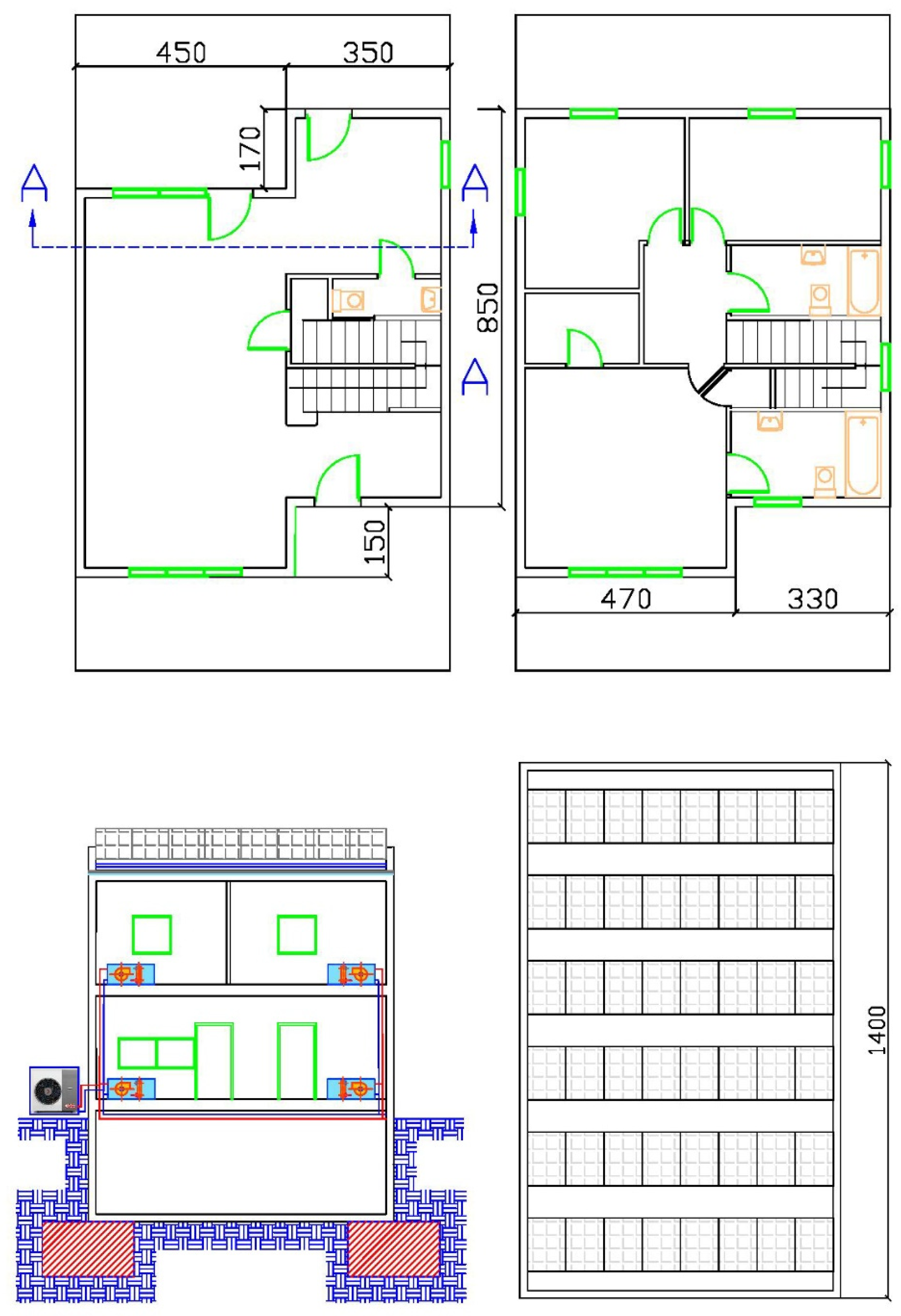
A detailed building and HVAC system simulation is carried out in the present paper for the reference house of Figure 1—a two story building with basement (insulation data in Table 1). The total floor area of the building is 221.81 m2, and the floor area of the conditioned zones is 141.81 m2. Ceiling height is 3 m. The house is located in Volos, a coastal port city in Greece, with latitude 39°:21′, longitude 22°:56′. The climate of the site is warm and temperate, with average monthly temperatures ranging between 8—10 °C during winter and 25–28 °C summer and about 500 mm annual precipitation [37]. It is a single-family, detached house with a level roof with 2 m overhangs at the northern and southern sides. The resulting large roof may be exploited for the installation of PV panels. In order to optimize the PV panels’ area and tilt angle for this specific building, comparative energy simulation runs are carried out for variable installed capacities and tilt angles of south-facing rooftop PV panels.
A plan view of the rooftop photovoltaic installation with maximum capacity is shown in Figure 1. The applied distance of 0.85 m between two consecutive south facing photovoltaic panel strings (portrait orientation, 1.65 × 0.99 m panels) has been proven adequate for minimal shading effect.
2.1. Building, HVAC System and PV Installation Modeling
A 3-ton capacity, (1 RT = 12,000 Btu/h = 3.6 kW) inverter driven air-to-water heat pump with scroll compressor is employed for space heating and cooling (SEER = 20, HSPF = 11). The heat pump produces a nominal 11 kW for heating (at standard ambient conditions of 7 °C) and 10.5 kW for cooling (at standard ambient conditions of 35 °C DB) [44]. The heat pump is connected to a hydronic heating and cooling distribution system with a fan coil unit for each space. The use of fan coils continues to be a good choice in Greece for a number of reasons: simplicity of installation and maintenance, possibility of retrofitting in older heating systems with oil or natural gas heating, where significant subsidies are available through EU funding. Efficient lighting by use of LED lamps and high efficiency (A+) electrical appliances are considered. TRNSYS 16 software was employed to predict the thermal and electrical performance and carry out a preliminary economic analysis of the reference building, located in Volos, Greece.
TRNSYS is a simulation program with a modular structure, well designed to solve complex energy system problems by breaking them down into a series of smaller components [45]. TRNSYS components (“Types”) are configured and assembled using a visual interface: The Simulation Studio. Building input data is also entered through a visual interface. Once the system components and their interconnection are specified, the simulation engine solves the resulting system of equations. New components may be developed and it is possible to embed components implemented using other software. The TRNSYS library includes numerous components and routines for weather data and forcing functions. It is well suited for detailed analyses of systems and is one of the simulation programs listed in the European Standards on solar thermal systems (ENV-12977-2). The TRNSYS “Type 56”, is compliant with ANSI/ASHRAE Standard 140-2001. TRNSYS is widely employed in building energy system simulations [6,42,46,47,48,49,50]. The performance of this software against experimental results and results of other standard tools for building energy simulation is well documented [51,52].
2.2. TRNSYS Simulation Details
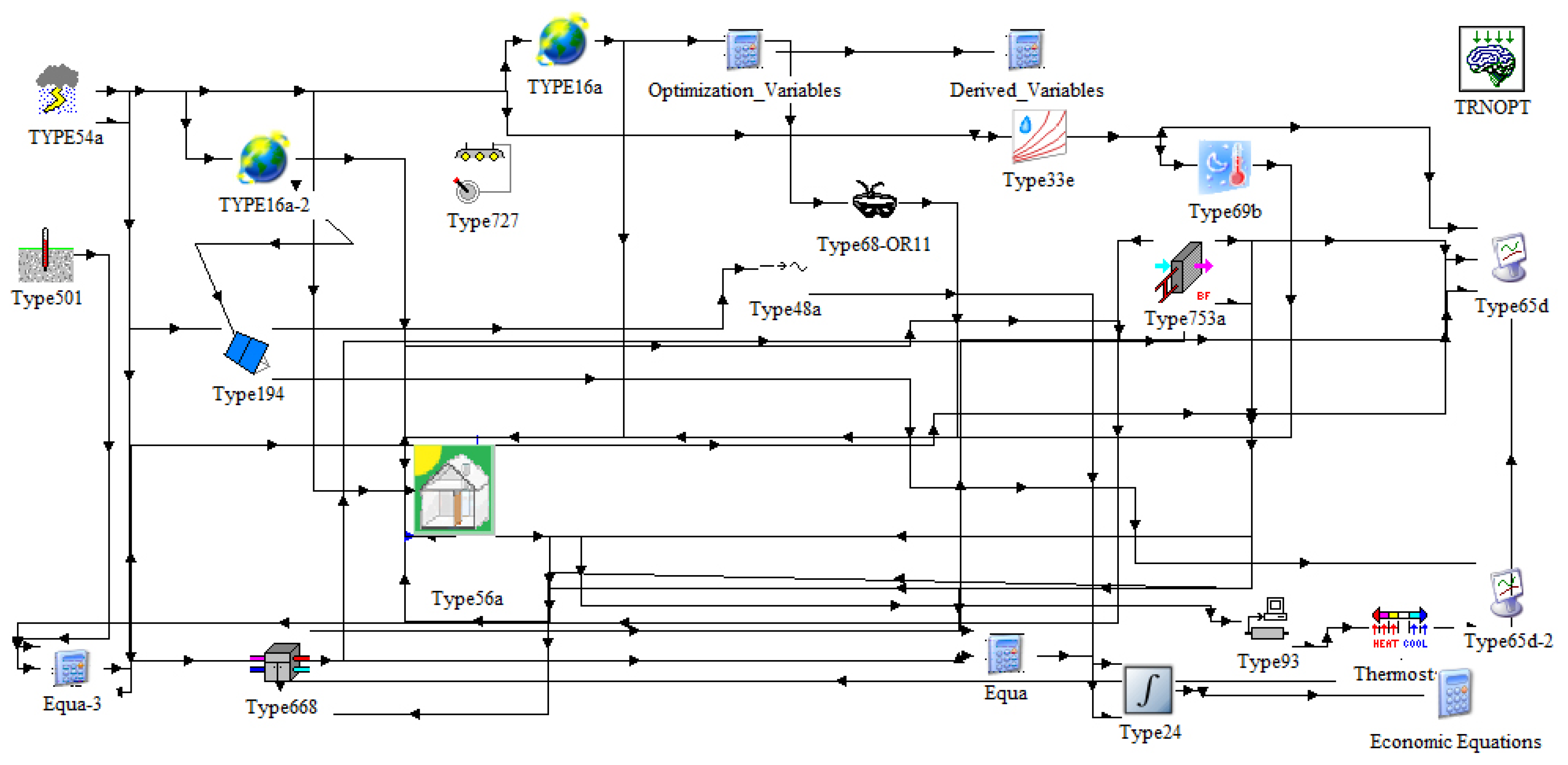
The system modelled is presented in Figure 2. It comprises a 3-zone building model of the reference house, employing an air-source heat pump for space heating and cooling. A rooftop PV installation is included. The HVAC installation comprises a hydronic distribution system with fan coils in the different parts of the house.
Apart from the standard utility components of the program, the specific TRNSYS component models (Types) employed in the simulations are listed in Table 2, along with several types belonging to the TESS library [53].
The information provided by the manufacturers [54], is not sufficient for detailed modeling of the PV-array. De Soto et al. [55] described a method to derive the PV module operating parameters based on the manufacturer’s data. The module is represented as an equivalent one-diode circuit based on the following five parameters: IL (the light current), I0 (reverse diode current), RS (module series resistance), RSH (shunt resistance) and a (modified ideality factor). The I–V curve is modeled by the following expression:
The modified ideality factor a is based on the cell temperature TC, the number of cells in series NS, the usual ideality factor ηI, the Boltzmann constant k and the electron charge q:
By using the I–V values provided in the manufacturer’s data sheet, the above equations can be solved for different reference conditions. By employing an existing EES plugin for TRNSYS Type 194, these parameters have been calculated to the values of Table 3. This is a high-end monocrystalline PV panel, as may be assessed by the unusual, almost ideal values of RS and RSH.
The main technical data for a single-phase inverter are presented in Table A2 (Appendix A). A 3-phase inverter is to be employed whenever the maximum of PV panels’ capacity is installed.
As regards the building envelope characteristics, the insulation values used, already listed in Table 1, adhere to current legislated standards in Greece. Double glazed windows are employed with U = 2.3 W/m2 K and g = 0.295 (Solar Heat Gain Coefficient). Window to wall ratio is 0.17. Ventilation rates comply with the requirements of ASHRAE 62.2-2004 [56]. Internal heat gains are according to ASHRAE [57]. The operation schedule provides uninterrupted heating or cooling of the house. The shading effect of two adjacent houses is also considered. Climatic data are inserted in the form of a Typical Meteorological Year (TMY) for the city of Volos. Hourly values of the following data are used: ambient temperature (DB), relative humidity, wind direction/speed, total/direct solar horizontal radiation. The HVAC control assumes a free-floating fan coil, that is, the fan coil heats the air stream as much as possible given the inlet conditions of both the air and the water streams [53]. The room thermostat controls zone temperature by switching on and off the air-source heat pump. The modeling of the air source heat pump is based on Type 668a [53]. The heat pump is employed solely for space heating and cooling. Domestic hot water production is done by a solar thermal collector, as required by Greek legislation. The heating and cooling mode characteristics of the heat pump are presented in Table A1. The reference size of the rooftop PV installation is 16 panels, arranged in portrait orientation in 2 rows of 8 Black Monocrystalline Standard panels each. Panel dimensions are 991 × 1650 mm and nominal output is 300 Wp (technical data in Table 4) [54]. Thus, the reference system is sized at 4.8 kWp. The maximum installation size that can be accommodated on the flat roof of the building would consist of 48 panels, (6 rows of 8), sized at 14.4 kWp (Figure 1). The number of 8 panels per row is only indicative. A variable number of panels per string may be accommodated by the inverter (see Table A2), thus the allowable number of panels is not necessarily modulated as integral multiples of 8. A year-round (8760 h) simulation with a time step of 0.1 h takes one minute of computation time on a PC with 8-core Ryzen 5 processor.
3. Results
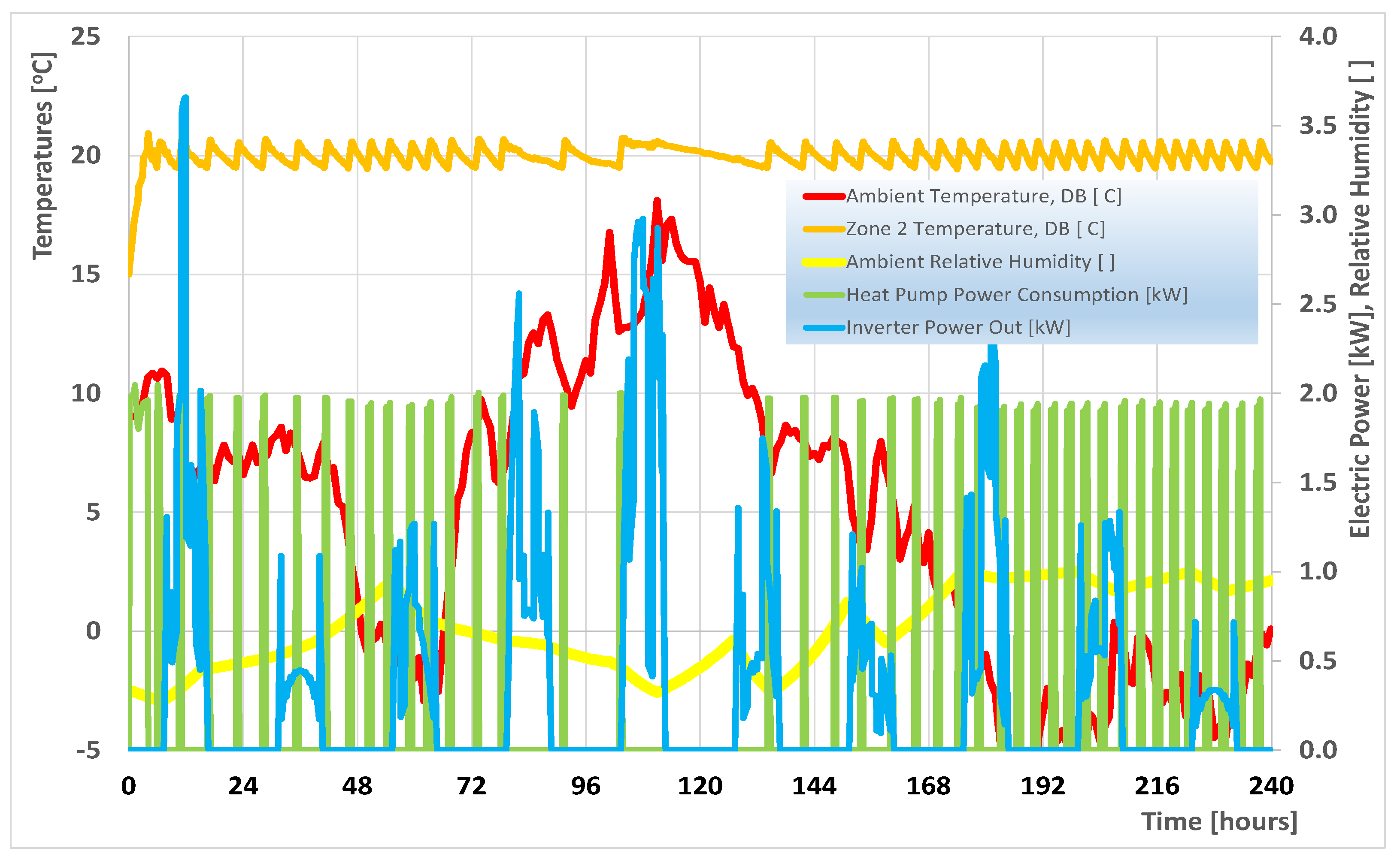
A graph of the simulated house’s winter operation, with the specific heat pump and a rooftop PV installation of 16 panels, is presented in Figure 3 for the first 10 days of January of the Typical Meteorological Year. The system’s control ON/OFF operation in heating mode is clearly observable.
During the first two hours, the room thermostat commands the heat pump to be always on, to heat the house up from an initial temperature of 15 °C. During this period, the heat pump is controlled by its own thermostat. After heating up, the room thermostat cycles on/off, keeping the room’s temperature at 20 °C ± 1 °C.
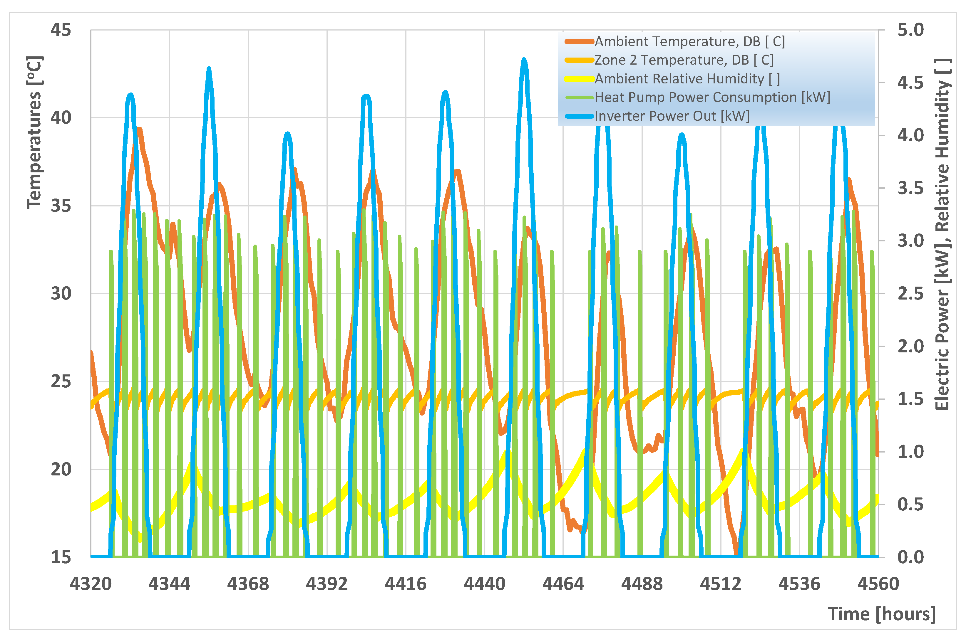
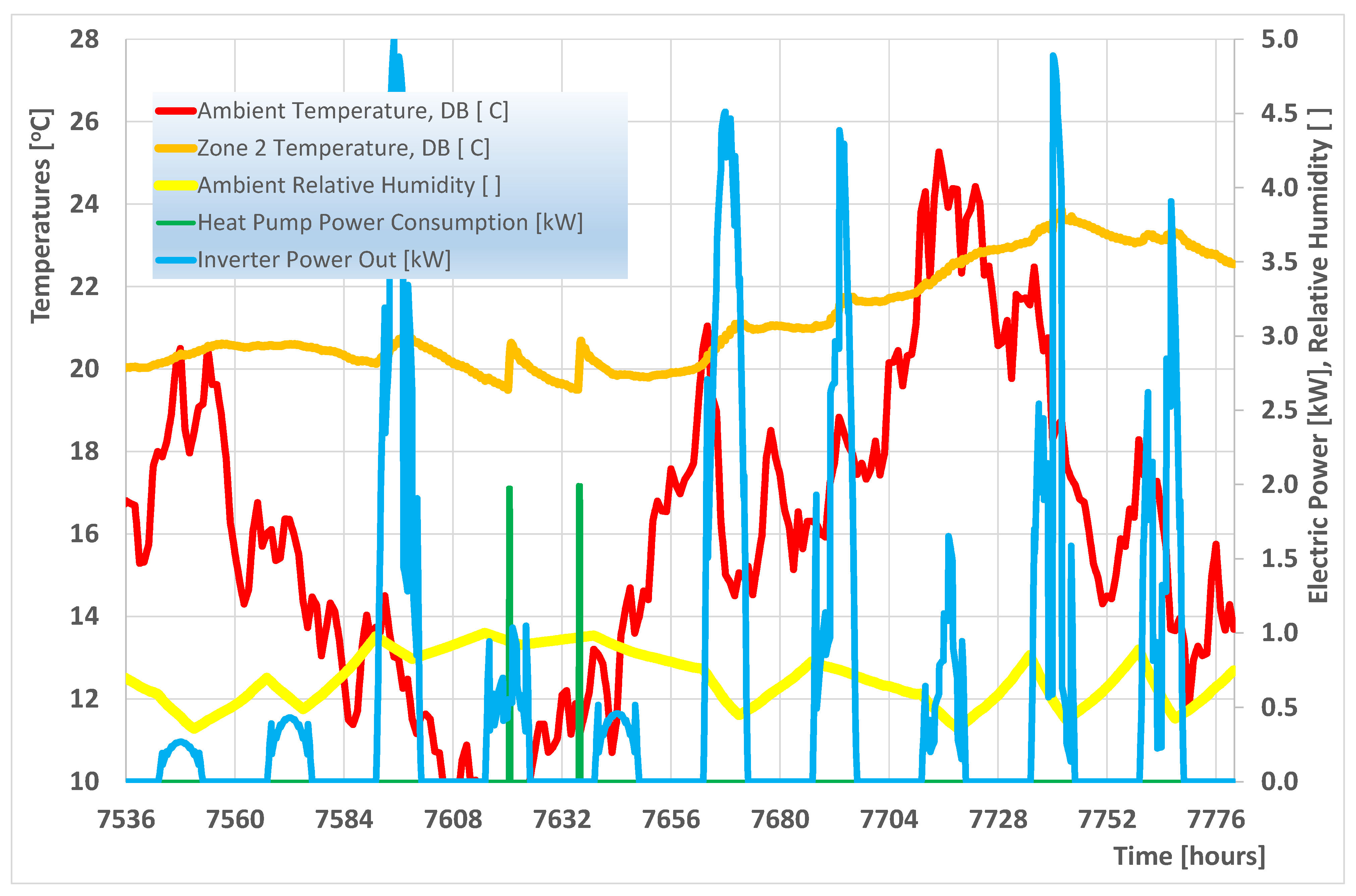
A graph of the system’s operation for the first days of July is presented in Figure 4. The heat pump control operation in cooling mode is observed. The onset of high ambient temperatures at about 4330 h is seen to increase the operation time and consumption of the heat pump during the hot hours of each day. This specific heat pump is more optimized for winter operation—for this reason its electricity consumption during the summer is observed to be higher. The heat pump’s operation becomes less pronounced when the ambient temperatures drop after 4460 h.
Figure 5 presents the transient performance of the system during ten consecutive days in mid-October, which is a neutral season for heating or cooling loads. The heat pump only needs to be switched on in heating mode for two short periods on the fourth and fifth day, (overcast days without sunshine), because the outdoor temperatures fell below 10 °C during the preceding nights.
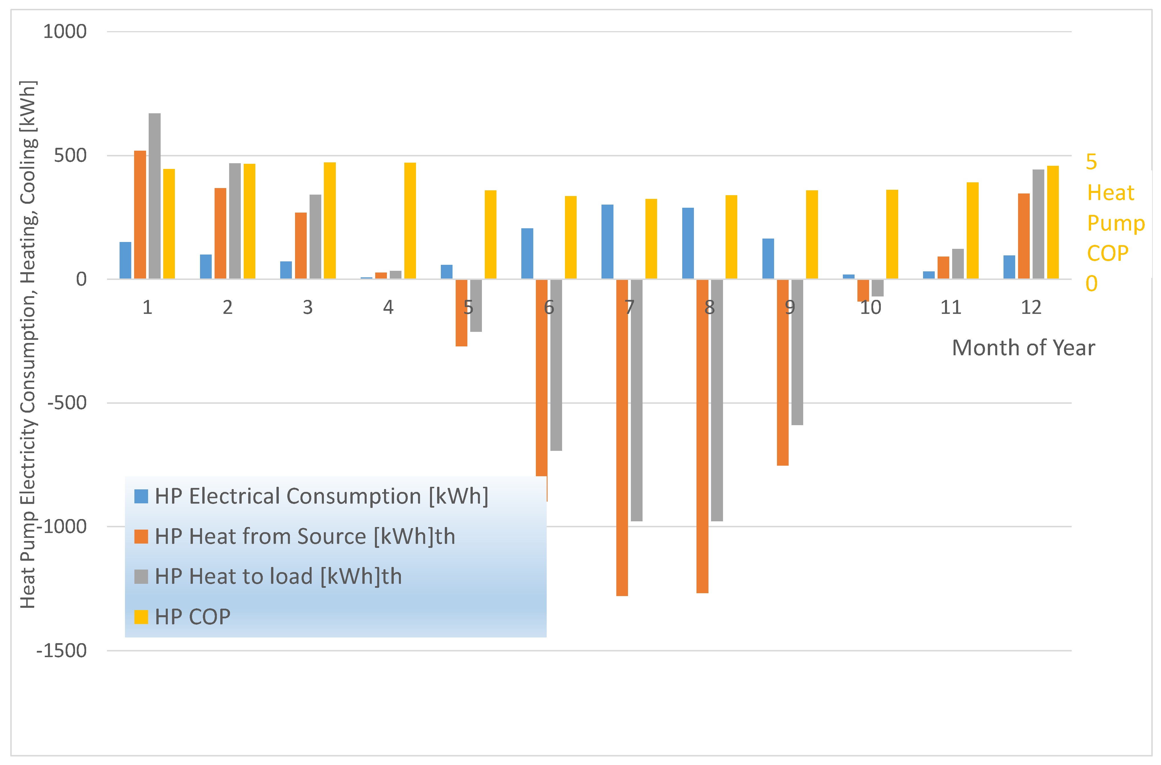
Next, we proceed to the calculation of seasonal heat pump heating-cooling production and seasonal Coefficient of Performance (COP) on a monthly basis, presented in Figure 6. Monthly average COP during winter is seen to vary in the range 3.9–4.7, whereas monthly average COP during the cooling season varies between 3.2–3.6. The cooling loads during the summer are considerably higher than the heating loads during the winter months. This is due to the prevailing climatic conditions on the site, with mild winters and relatively hot summers.
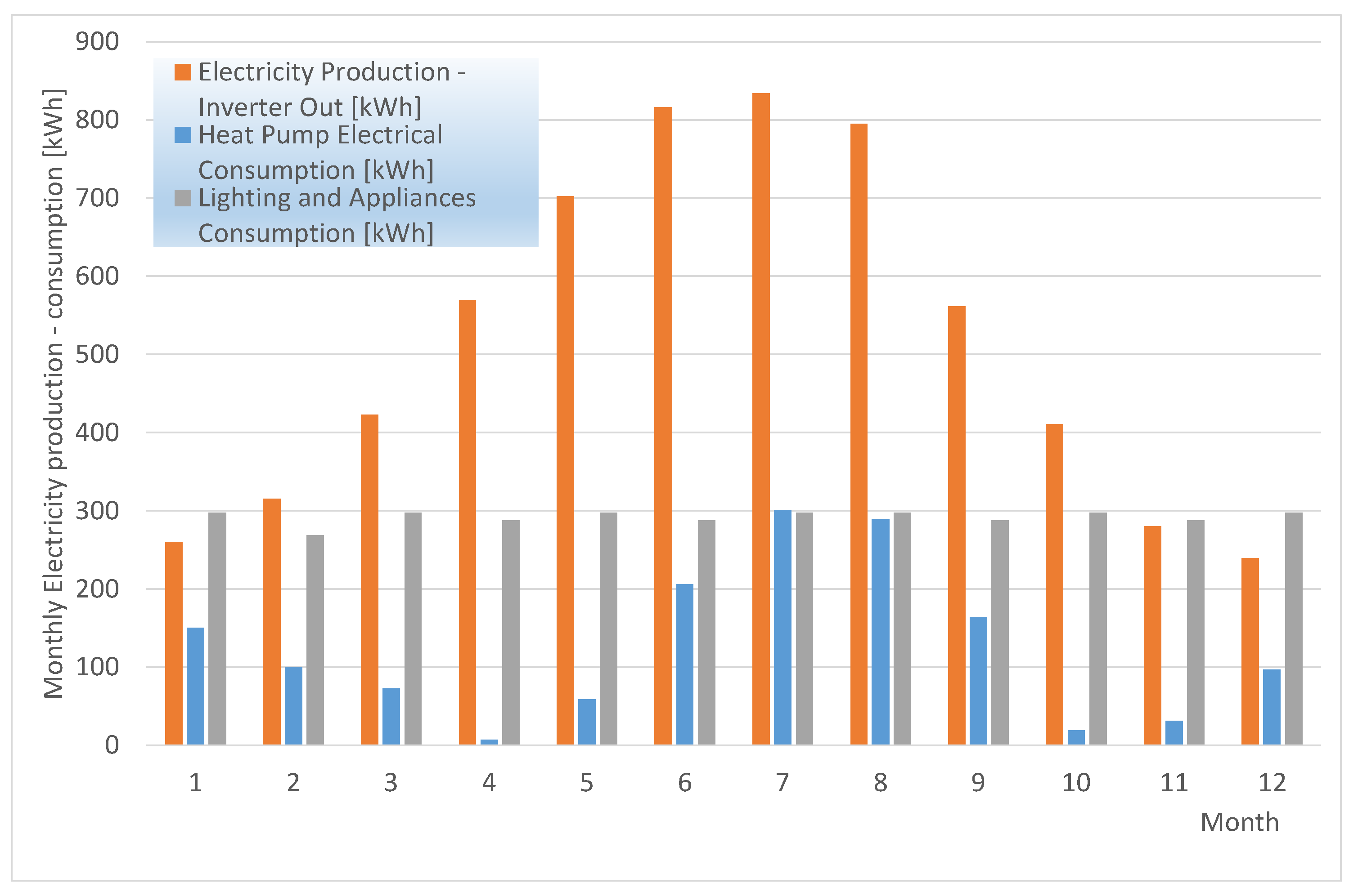
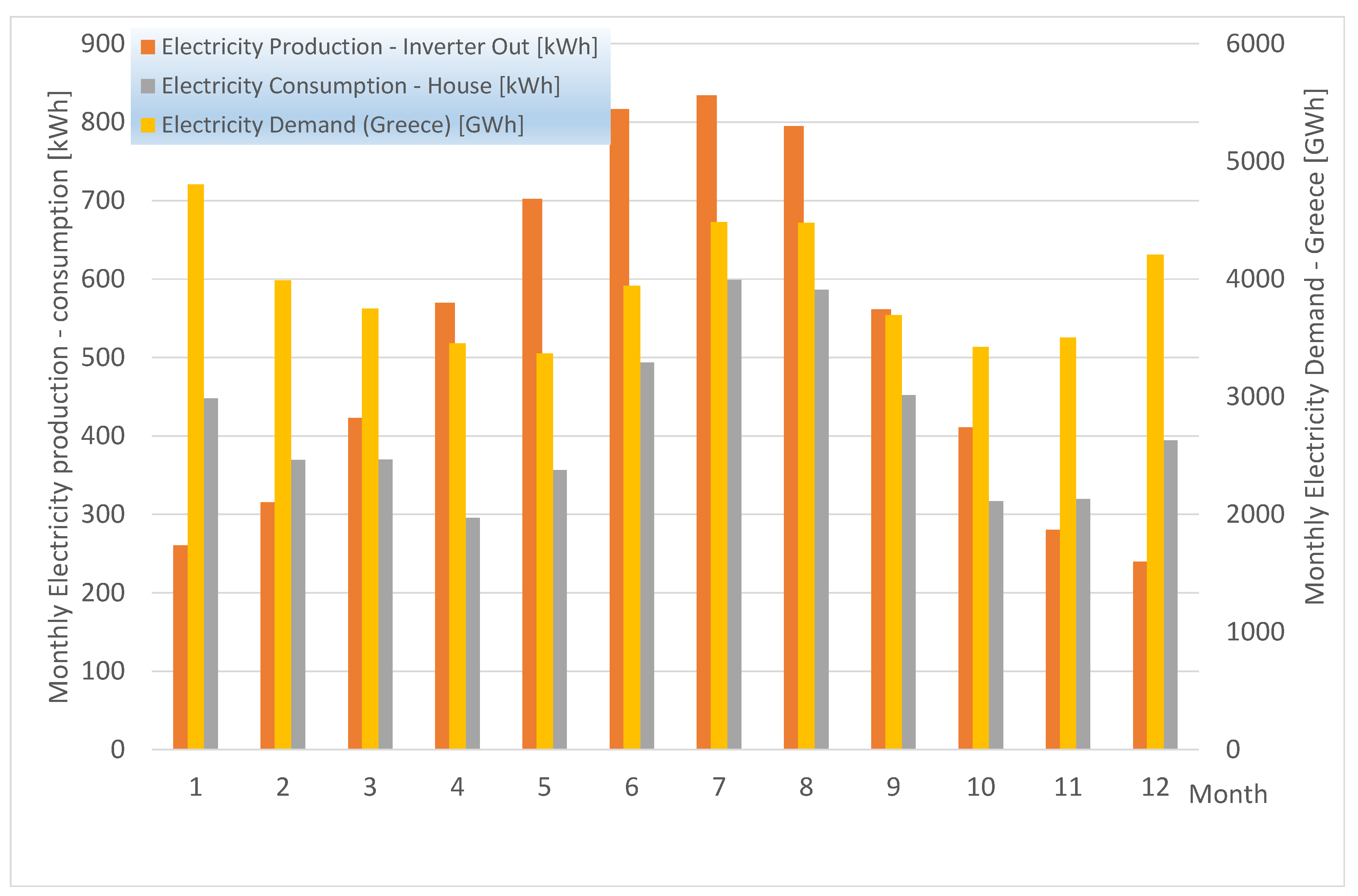
The monthly electricity production and consumption summary during the year is presented in Figure 7, with a reference size of 16 PV panels. The total annual electricity consumption of the house amounts to 5000 kWh, or about 35 kWh/m2 y. This is a low consumption compared to the average electricity consumption in Greece, despite the fact that oil and gas are mainly used for space heating [58]. A requirement for a passive house would be to consume less than 120 kWh/m2 y primary energy consumption, which is about the same level [59]. For comparison, the share of final energy consumption in the residential sector in Greece (2016) was 63% for space heating, 7% for water heating, 9% for cooking and 22% for electrical appliances (including space cooling) [60]. One may observe that this size of high efficiency PV installation already results overall in a zero-energy house, based on the annual electricity balance. However, on a monthly basis, one may observe that during the winter months, the house would produce less electricity that it would consume. On the other hand, during the summer months, the house’s electricity production significantly outperforms its electricity consumption, despite the fact that this consumption is maximum during these months (as already observed in Figure 6 and as will be further discussed in the context of Figure 8).
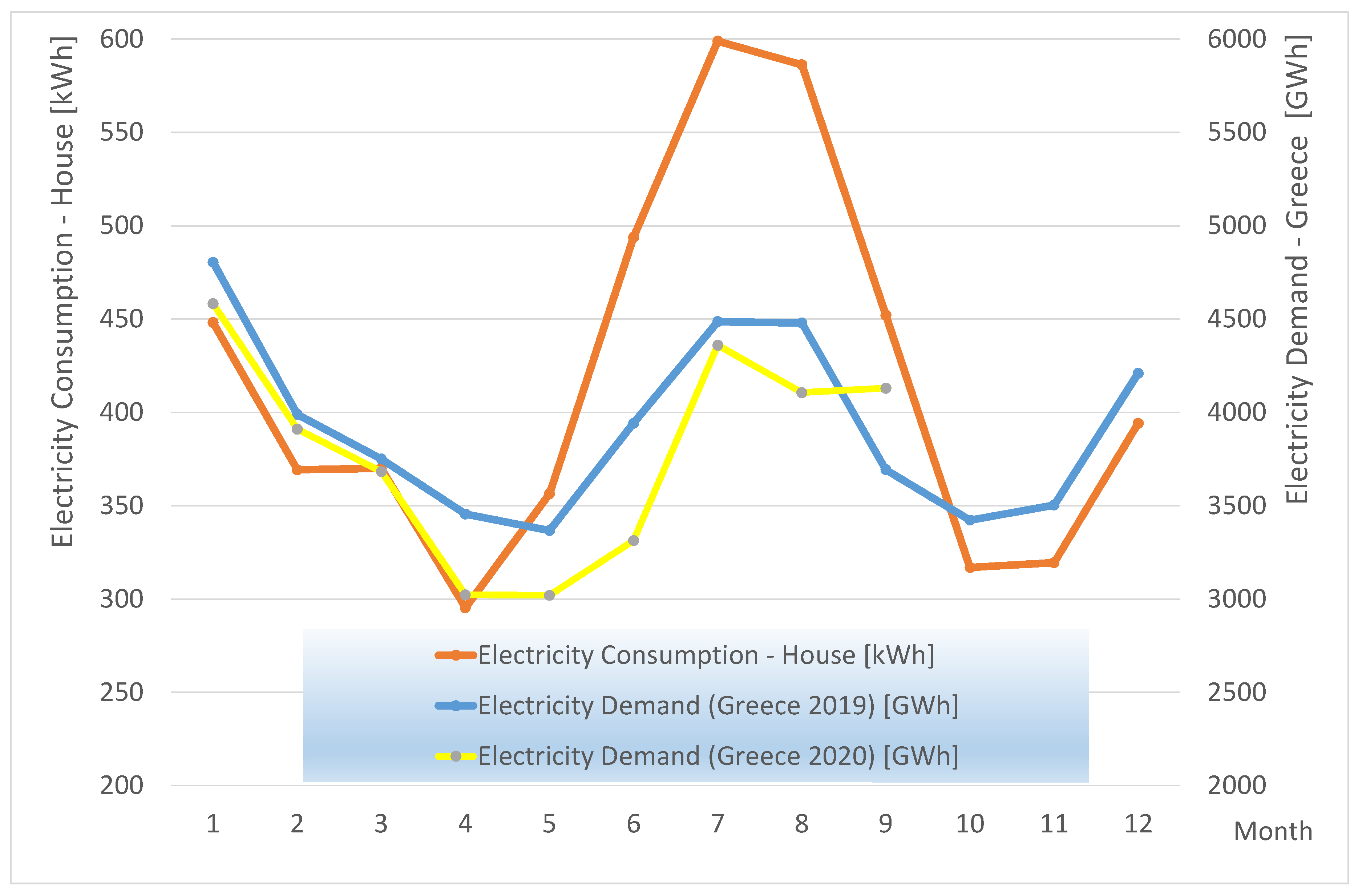
The monthly variation in electricity consumption of the specific house, as simulated based on a TMY, is compared in Figure 8 with the monthly variation of electricity consumption in Greece in 2019. The monthly electricity consumption of Greece is also presented for the first 9 months of 2020, in order to draw some useful conclusions about the effect of tourism on Greece’s electricity consumption during the summer months. It is interesting to observe that the COVID-19 shutdown in Greece resulted in significant reductions in the monthly electricity consumption only for the months of April, May and June. The consumption during July was similar to the 2019 levels, and August was associated with a smaller reduction. This would imply that the effect of tourism on the electricity consumption of Greece is much less pronounced than one would intuitively expect.
Now as regards the house, since the heat pump operation contributes significantly to the electricity consumption, we observe peaks during the summer and winter, with lower levels during the neutral months of spring and autumn. The same trend is followed by the monthly electricity consumption of Greece. However, the summer peak is significantly higher than the winter peak in the house’s consumption. This is due to the local microclimate with very mild winters but hot summers, and the fact that the specific heat pump’s efficiency is more optimized for the heating mode. On the other hand, the electricity consumption peak for the house coincides with the electricity production peak of the PV installation, which is favorable on self-sustainability grounds, if long term electricity storage is included.
3.1. Rooftop PV Installation Size Optimization
As already discussed in previous sections, in countries with high solar potential, while the upfront costs of a new home will be increased by the installation of rooftop PV panels, the savings benefits for the homeowner outweigh these initial costs. However, it is interesting to see if the size of the PV installation could reach the maximum permissible PV area based on the roof area, or if there exists an optimal size based on the specific cost–benefit assumptions to be adopted.
Starting from the initial cost, one may use an indicative cost assumption of USD 3.00 per watt (peak) of the installed solar panel system [61]. Obviously, the system size is constrained by the available rooftop area. Based on a typical calculation and taking into account the shading effect between the series of panels, the maximum allowable installation size is 48 panels (6 series of 8 panels each). Furthermore, the cost would have a tendency to drop with the installation size. For this specific study it was assumed that the above-mentioned cost of USD 3.00 per watt (peak) of installed panels will drop to USD 2.50 per watt (peak) if the maximum size of 48 panels is installed, and this drop is assumed to be proportional to installation size [61]. As regards the annual operation and maintenance costs, these would include the scheduled maintenance/cleaning of the panels, any unscheduled maintenance and an inverter replacement reserve, amounting to a total of USD 0.05 per watt (peak) of installed panels [62].
Next one should focus on electricity savings due to the rooftop PV installation. Here, there exist differences in tariffs among different countries and net metering policies. However, an indicative assumption could be that the home owner will save at an average electricity price of USD 0.20 per kilowatt-hour (kWh), produced at the inverter’s outlet, for the part of the demand covered by PV generation. On the other hand, it is reasonable to assume a lower electricity rate of, say, USD 0.10 per kilowatt-hour (kWh), for the excess electricity produced [63,64]. This difference is due to the fact that the first kilowatt-hours are—more or less—directly consumed at house level, without loading the electricity distribution system [14]. On the other hand, the kilowatt-hours produced beyond the average house consumption must be fed to the distribution network and it is reasonable that the producer would receive a lower price. The reference time for the energy balance calculations for the pricing of these electricity amounts is set to one year, for the sake of simplicity.
As regards the efficiency deterioration of the PV panels from year to year, we will assume an average annual drop of efficiency by 1% of its average value for the previous year, based on experience from monitoring similar types of PV panels [65].
The above indicative figures are to be employed in the development of the objective functions for the optimization. Another important assumption that must be taken into account is the cost of the money that may be deployed by means of the net present value (NPV).
The net present value is commonly employed to express the value of future income from a solar installation. It is computed by subtracting the initial investment from the sum of the total discounted future cash flows over its lifetime, which is the present value of future cash flows, calculated using a discounted rate. In our case, the negative cash flows are the costs of the project, comprising the PV installation, the ongoing maintenance and the electricity purchased form the grid. The positive cash flows are the benefits to the project: the surplus electricity from the PV sold into the grid as the feed-in tariff and the financial savings due to self-consumption of PV electricity—thus avoiding the costs of purchasing electricity from the grid. As regards the last benefit, the NPV of the project is of the house with PV installation and heat pump heating and cooling, in comparison to an identical house but with no PV system. For the house without PV installation, all electricity would be purchased from the grid at the above-specified tariff. Hence, for the house with PV installation for the self-consumed component of the electricity demand—there is a benefit in comparison to the house with no PV—equal to the negative of the financial cost of purchasing the self-consumed component of the electricity demand.
The net present value may be calculated using the following equation:
where N is the lifetime of the installation (assumed to be 20 years); i is a specific year in the lifetime of the PV installation; Cash_Flow for year 0 is minus the system cost; and for years i = 1 through 20 positive cash flows are the electricity savings and profits as explained above, and negative cash flow as the operation and maintenance costs. The investment tax credit, which is normally applied in year 0, is neglected in this calculation. d is the discount rate, assumed here as 1.5%.
The initial calculation will assume that the money for the initial investment is paid by the home owner as an alternative means of investing his/her savings.
Based on the above assumptions, the net present value of (3) is employed as the objective function for the optimization process.
The optimum area of installed PV panels will maximize the NPV of the investment. The selection of US currency for this study is based on the following energy economics facts: (i) the ever decreasing prices of photovoltaic panels are driven by China, which has its currency pegged to the US currency; (ii) the prices of natural gas, which affect electricity prices, are also in US dollars. Thus, the economic data produced by this study will be more widely relevant.
3.2. Size and Tilt Angle Optimization by Genopt
The performance summary for each month of the year with the initial reference installation size of 16 panels is presented in Figure 9. According to these results, the electricity produced by a total of 16 PV panels (which is close to the optimal size), is comparable to the total electricity consumption of the house (heat pump + lighting + equipment).
The type of simulation demonstrated here allows for optimal sizing of the PV installation, for the specific building envelope construction and heat pump quality. In this way, it can be a valuable tool for the design process [66]. Moreover, the use of this type of modeling allows us to assess the effect of variable electricity pricing during the day
The optimization is carried out by the GenOpt optimization software, produced by Lawrence Berkeley National Laboratory (LBNL). The interfacing of TRNSYS with the GenOpt software is made by TRNOPT subroutine (Thermal Energy System Specialists, LLC). TRNOPT is an interface code between the two piece of software which tailors the optimization process to the programmer’s needs. Thus, the process of optimizing the TRNSYS simulation results just requires the selection of a TRNSYS input file, the selection of the variables which will be allowed to vary, the choice of the optimization algorithm and the choice of the objective function.
The following variables are varied during the optimization process:
- Total installed area of PV panels (number of parallel loops of series connected panels)
- Tilt angle of the south-facing PV panels
Optimization is made by use of the Hooke-Jeeves method, tilt angle is allowed to vary between 10 and 50 degrees and system size between 8 and 48 panels.
To demonstrate the effect of different electricity pricing policies, we are going to apply the above-mentioned methodology for the economic analysis of the rooftop PV installation. Starting with the reference size of 16 panels with 4.8 kWp capacity, Figure 9 presents the monthly electricity production of this installation, along with the monthly electricity consumption of the house, which includes the consumption of the heat pump, lighting and appliances of the house. The annual electricity consumption is about 5000 kWh, which is only 25% higher than typical single family houses in Europe with gas heating [14]. The monthly electricity consumption of Greece in GWh is presented for comparison in the same figure.
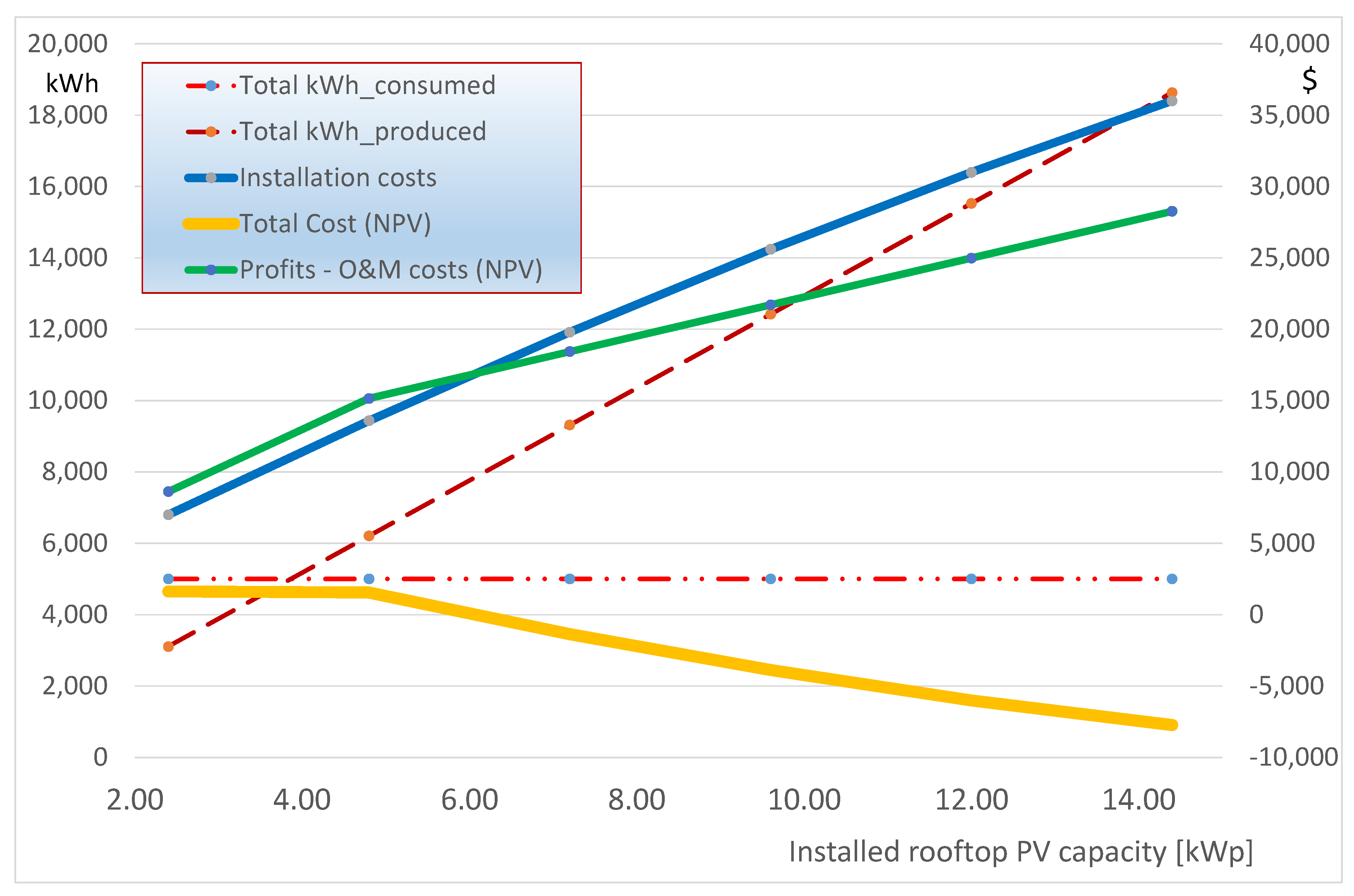
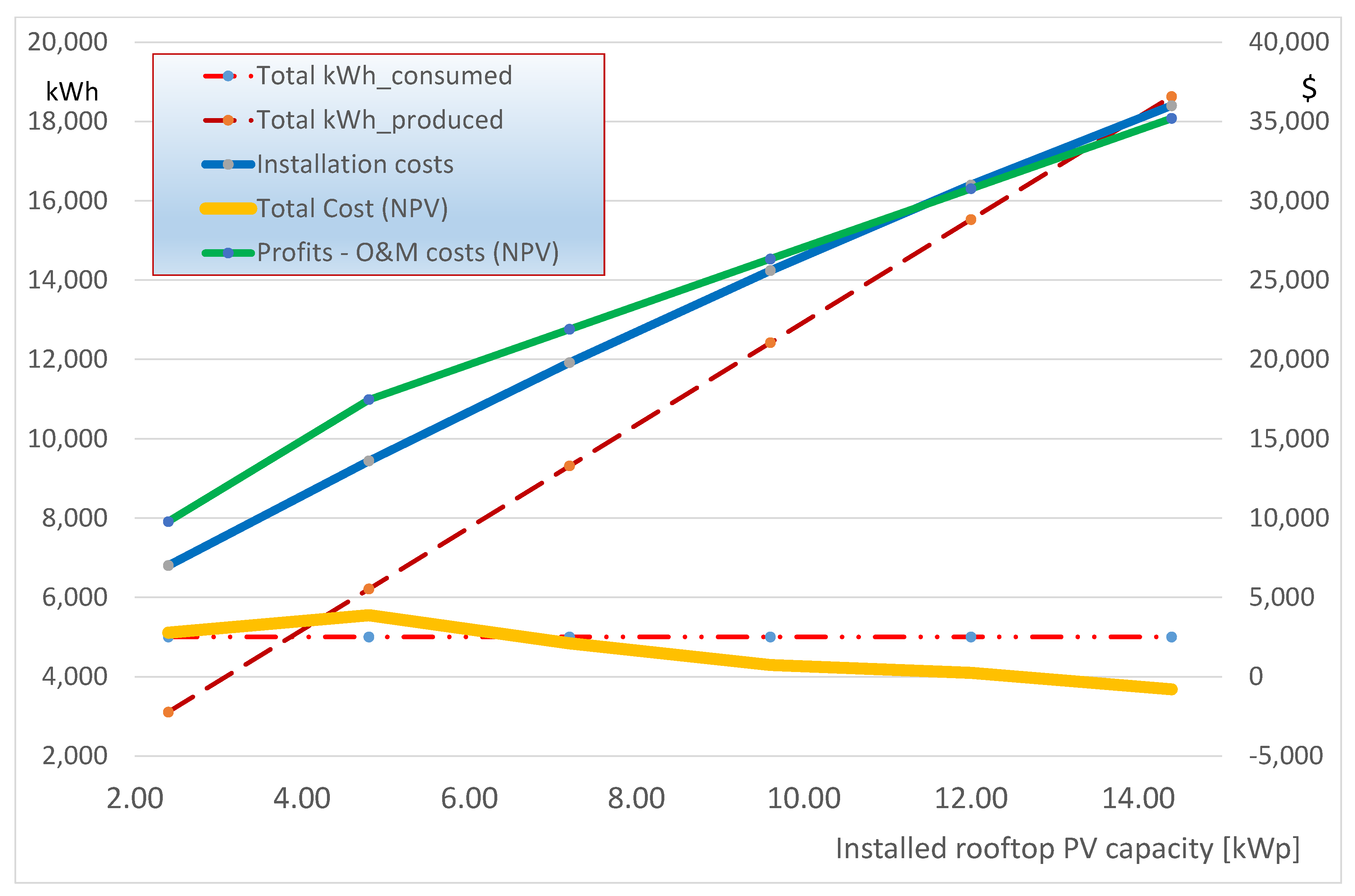
The results of the system’s annual performance are presented in Figure 10. For ease of understanding the tilt angle is set to the optimal value of 30 degrees, which resulted from the optimization process. The rooftop PV installation size is varied from 1 to 6 strings of 8 panels. This corresponds to 8 to 48 panels of 300 Wp each. The annual electrical kWh consumed are constant, since the house and heat pump system are not modified between runs. However, the system’s electricity production is increased with the number of panels installed and the same is true for the initial capital cost of the rooftop PV installation. The net present value analysis is carried out for a lifetime of 20 years. According to these computations, the NPV of cash flows from electricity production minus operation and maintenance costs increase faster than the equipment cost, until the PV installation size rises to 4.8 kWp. This size is capable of covering the annual electricity consumption of this specific house. If the rooftop PV installation size increases above this figure, the trend is reversed and when one exceeds a capacity of 6 kWp, the NPV of the investment becomes negative, which means that under these specific assumptions it is not profitable to install more than 6 kWp without some kind of financial subsidy. The above figures are in general agreement with the results of other studies utilizing dynamic building simulation software [13], or more simple standardized techno-economic software tools as the NREL’s system advisor model (SAM) [67]. Based on the above results, an alternative approach that would accelerate rooftop PV installations without any form of subsidies, would be to allow small rooftop PV capacities to feed directly to the houses’ internal electrical installations, without requiring a second electricity power meter and the associated net metering contracts.
4. Discussion
As already reported in the Introduction, California is a pioneer in the mandatory installation of rooftop PV panels in all new houses since the start of 2020. It is also a pioneer in house electrification (the shift here was also from natural gas to heat pumps for heating). In an analogous manner, Greece has the opportunity to become a pioneer in Europe in house electrification and the production of electricity mainly by renewables. There are significant similarities regarding the climatic conditions (high sunshine and mild climate; the urban areas of San Diego or Los Angeles are comparable with seaside cities in central and southern Greece). Of course, the house construction and building materials are different, but the heat pump and photovoltaic technology is international.
It is interesting to compare the optimal size of the PV installation computed above to the one suggested in the Compliance Manual for the 2019 California Building Energy Efficiency Standards [68] for a house of similar size and climate. According to this document, the following equation is employed for Title 24 to calculate the minimum required solar panel system size in peak kilowatts (DC):
where CFA is the conditioned floor area of the house in square feet, NDwell the number of dwelling units (equal to one since this is a single-family house) and A and B adjustment factors based on the climate zone of the building. For our specific site the values of A = 0.6 and B = 1.2 could be assumed, corresponding to the shoreline climatic zones 5 or 6 (central California). Since the conditioned floor area of the house is 140 m2, the above approximate calculation gives a PV size of 2.15 kWp. Since the PV modules employed in this study are 300 Wp, the required size for the installation would be close to 8 panels, (2.4 kWp), with a total area of about 13 m2. It is observed that the optimal size of the installation computed by the above optimization study is about twice the minimum size set by the California solar mandate for similar climatic conditions.
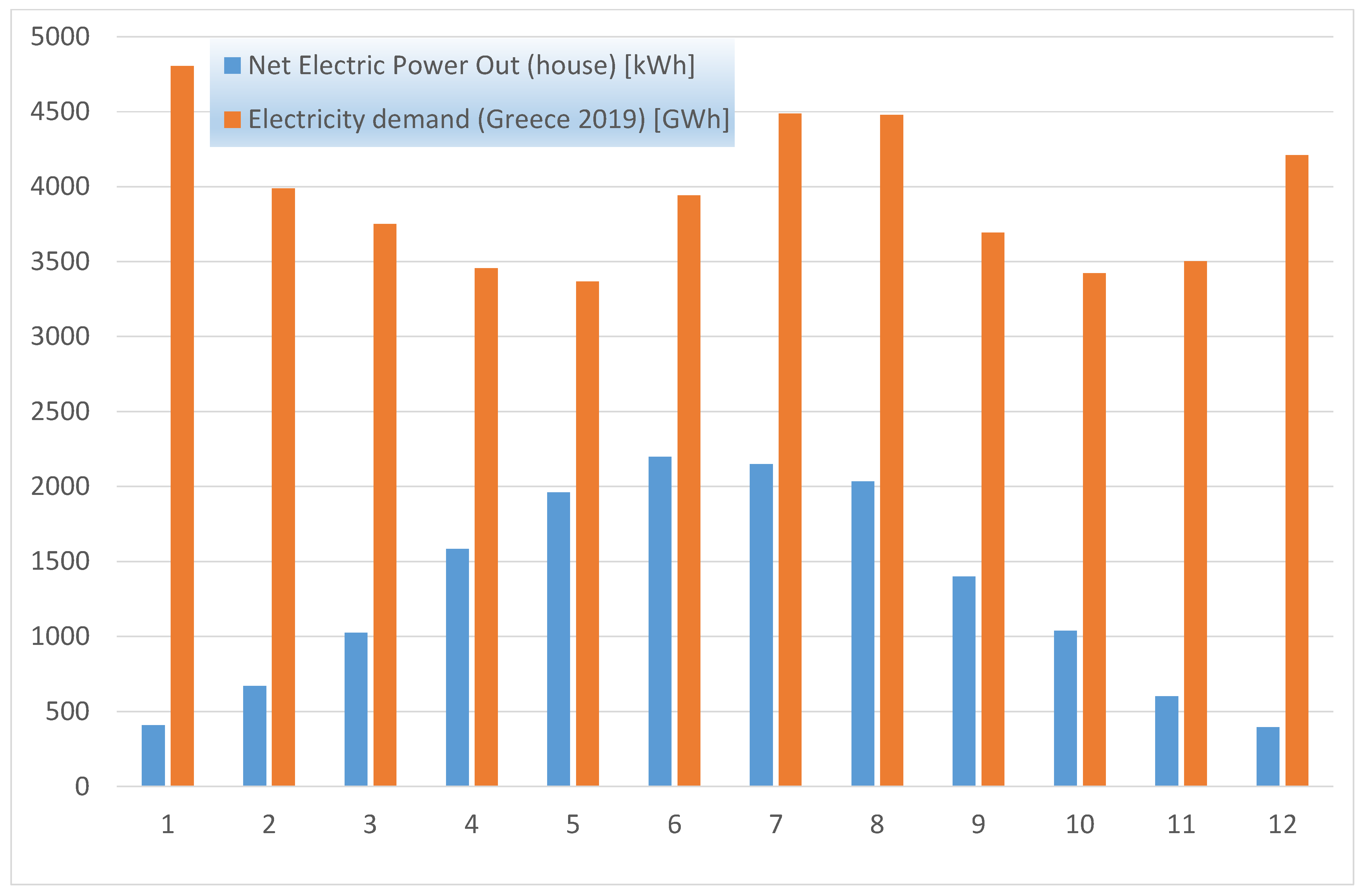
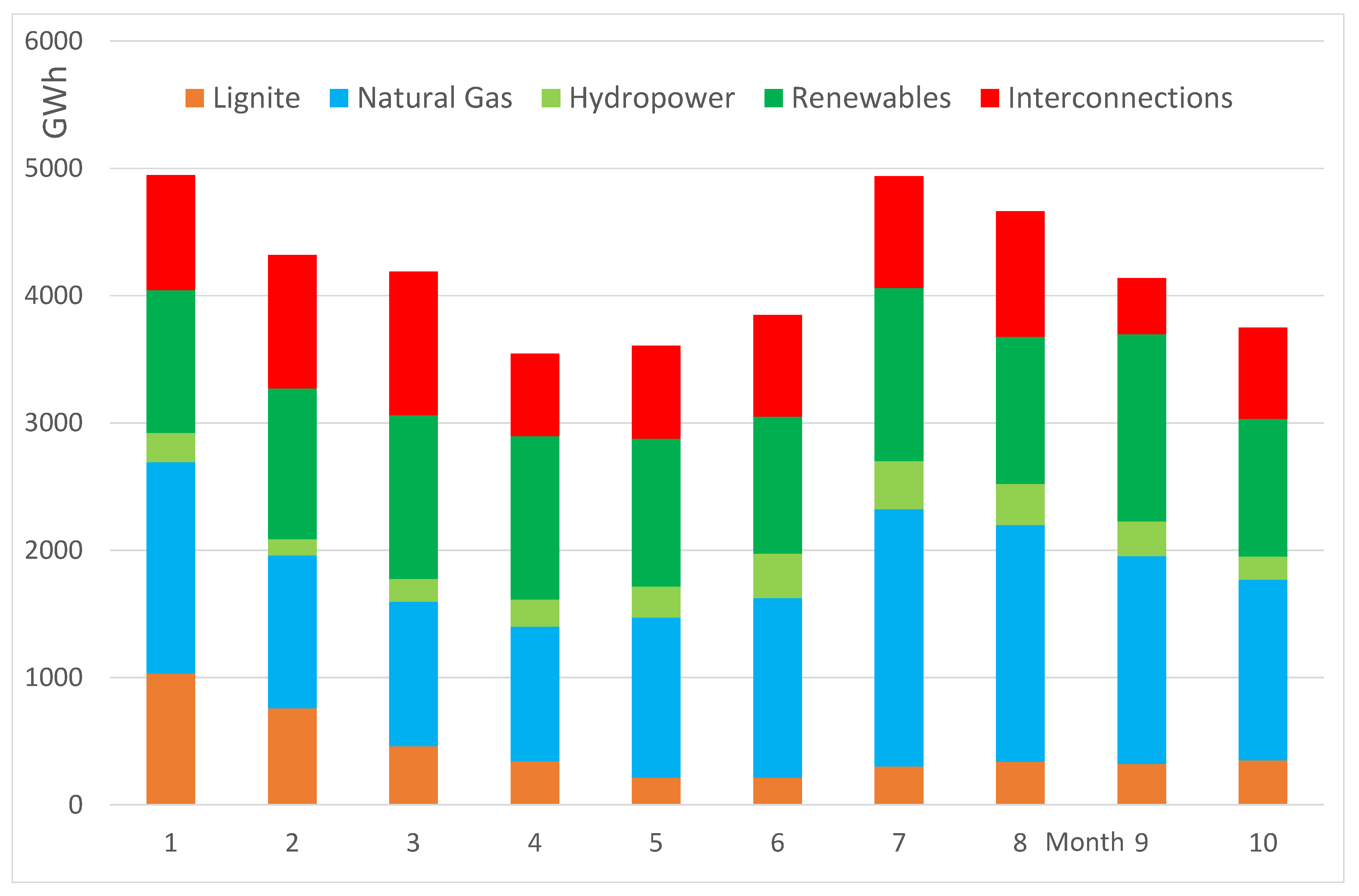
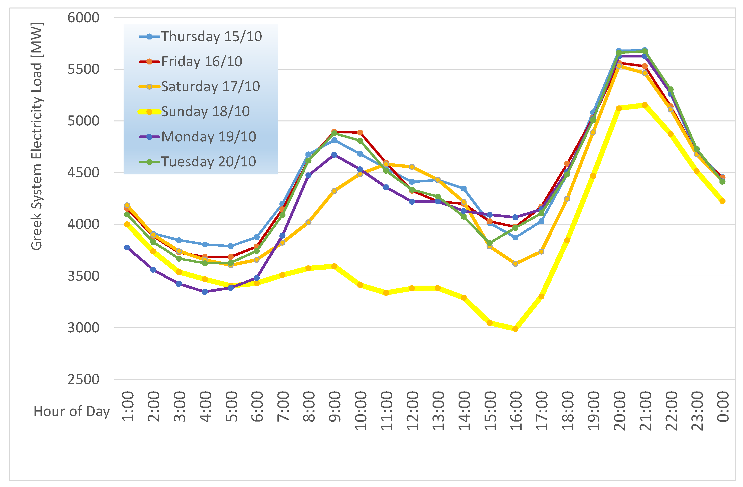
On the other hand, one may observe by a comparison with Figure 1, that the optimal size of the rooftop PV installation is significantly smaller than the installation capacity for a house with a flat roof. There is more room for installation even for a house with an inclined roof. Figure 11 presents the monthly variation of the net electric power that can be sent to the network if this specific house is installed with the maximum possible capacity of 48 panels on its roof. Moreover, on the same figure we plotted the variation of electrical power consumption of all Greece for 2019 (the year before COVID-19). It can be seen that the maximum permissible rooftop PV installation size may supply electricity to the grid that is desperately needed, especially during the summer months. If we look at the balances of incoming—outgoing electricity in the 400 KV interconnection transmission lines with its neighboring countries, Figure 12, it is apparent that under the current circumstances Greece is a net importer of electricity.
Greek net imports of electricity have significantly increased and constituted 20% of total electricity consumption during the first 10 months of 2020. It is interesting to examine the possibility for a part of these electricity imports to be replaced in due time by electricity produced from additional privately owned PV installations. As induced by systematic observation of the daily evolution of hourly electric power imports from the 400 kV interconnection lines [70], significant imports in the power range from 300–500 MW occur during hours from 08:00–14:00, which are hours of the first peak that is normally observed in the Greek electricity system’s load curve during the working days (Figure 13). According to this figure, during the neutral season, a maximum ramp rate of about 0.5 GW/h is observed between the hours 07:00–08:00 during the morning ramp-up. The increased installation of photovoltaic units assists the electricity grid to face this ramp rate with reduced employment of flexible power plants as open cycle gas turbines. On the other hand, the gradual increase in heat pump units in the process of heating electrification has a certain effect on the morning, and especially the evening ramp, which interesting to study in more detail by means of field measurements and transient simulations [71].
4.1. Effect of Net Metering Policy on the Rooftop PV Installation Rate
As already observed in the results of Figure 3, Figure 4 and Figure 5, the time between the hours 08:00–14:00 is associated with significant production capacity by PV installations. Thus, the economy-driven increase in rooftop PV installations in new and existing houses in Greece could help to bridge this morning gap during the period of fast-track closure of lignite-fired power stations.
Of course, there exists one bigger peak in the daily electricity demand of Greece (Figure 13), which cannot be addressed by photovoltaics, since it happens during the evening hours. Now the discussion should shift to the economic profitability for the house owner for installation of higher capacity rooftop PV panels. As already discussed in the context of the optimization in Figure 10, the installation of a PV capacity exceeding 7.2 kWp, under the specific net metering tariff, crosses the break-even line and makes the investment unprofitable.
On the other hand, we have already seen that the profitability is marginal under the current installation costs without some form of financial motive or subsidy. However, it should become clear by the above discussion that the introduction of flat subsidies per kWh produced is not an easy to implement solution, because the period of effect of the subsidies extends for many years and this would require the rate of subsidies to be updated every two or three years. This practice produces an uneven playing field for the investors. What is needed here is to minimize the level of the subsidies by a more accurate assessment of their effects on the daily grid operation. Since our purpose this time is to further increase installed PV capacity at a fast rate by private investment, the optimization process can be modified to examine the effect of smart electricity pricing, with a somewhat higher price to be paid to the house owner for net electricity supplied to the network by the PV installation during the previously mentioned hours of day between 08:00–14:00. For the net electricity transferred to the network during this 6-h peak demand period, it would be reasonable to pay an additional premium of USD 0.03 to the owner. To address this optimization problem, the availability of a transient simulation of the house’s energy system’s performance is essential. That is, the added complexity of the physics-based building and energy system’s model employed in this study is capable of performing this type of calculation, which is not possible with other packages that are based on statistically derived predictive regression models, predicting energy consumption and production based on a few common weather-based factors.
The results of this new pricing policy for the electricity transferred to the network by the rooftop PV installation for the 20 year lifetime performance of the system are presented in Figure 14. Under this alternative policy, one can observe that a bigger PV installation becomes profitable. This will be further assisted by the continuously decreasing installation price of photovoltaic panels. To this end, it will be necessary to further improve the rules of net metering in Greece, especially to reduce the reference interval for calculating the feed-in tariffs, which is currently three years and thus causes a degree of uncertainty for the prospective investor.
4.2. Financing Possibilities by Extension of Housing Mortgages
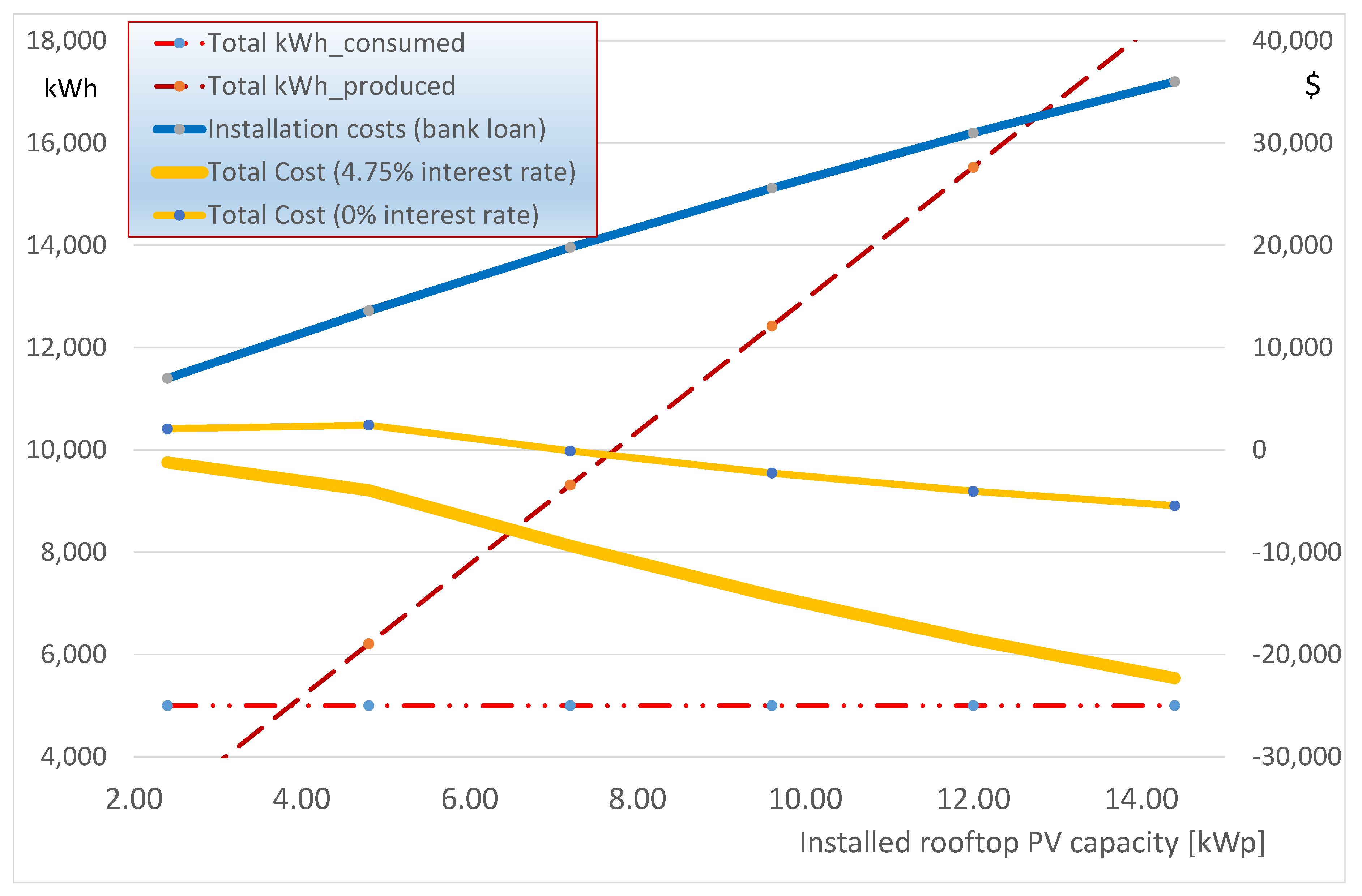
As already reported in the introduction, the regular practice in California is to extend the mortgages of new houses to include the additional financing required for the rooftop installation. In this section, the detailed model’s results are employed to calculate the required additional monthly installment for the financing of the installation by a bank loan. The resulting monthly mortgage payment would be USD 45 for the installation of eight panels, (2.4 kWp) but this would be reduced to USD 30 for the same size if a zero interest rate were to be applied as a means of government financial incentive.
If zero interest loans are available for this investment, the results of Figure 15 indicate a negative NPV for a rooftop PV installation capacity of 7.2 kWp. That is, for a new house, the owner may finance the rooftop PV installation by an extension of his/her mortgage contract, which would be recuperated by the reduced electricity bill. Even bigger installation sizes would become profitable with variable electricity pricing (an additional premium for electricity sent to the grid during the daily hours of peak consumption), as already investigated in the context of Figure 14. Further decreasing prices per Wp of PV panels would enhance the profitability of this type of investment.
5. Conclusions
A detailed, transient simulation of a house’s HVAC system operation along with the electricity production of the rooftop PV installation was carried out to shed light on the effect of installation sizing on the system’s performance, and the daily and seasonal balance between electricity consumed and electricity supplied to the network. Size and tilt angle optimization of the PV installation was carried out in the framework of emerging policies aiming at a significant increase in renewable electricity in Greece. An analysis of the electricity demand from the Greek power grid was comparatively presented, to find the periods during the year that rooftop PV electricity could support the process of transforming the Greek power system away from the reliance on fossil fuels.
To this end, the economic viability of installing rooftop PV panels was examined under different electricity pricing and equipment financing scenarios.
Under the basic pricing scenario, the installation of up to 4.8 kWp capacity was found profitable for a 20 year lifetime for a house owner who invested his own money in this project. The optimal tilt of the south-facing PV panels in this context was found to be 30 degrees. This resulted in increased electricity production during the summer, which matches the increased needs of the Greek electricity market.
The most interesting result of this study was the prediction of the effect of variable electricity pricing in net metering. This was demonstrated in the example of a premium to be paid for electricity produced during the hours 08:00–14:00, which are peak hours for the Greek system. Under this scenario, it would be profitable to further increase the total size of rooftop PV installation up to 12 kWp, which is close to the maximum capacity of the flat roof of the house. Such policies would speed up the already significant increase in renewable electricity in the Greek system, which is currently phasing out its lignite-fueled power plants at an accelerated pace. These results could be employed in the more rational design of the net metering tariffs to support further expansion of rooftop PV systems in new and existing buildings. Building electrification, along with the installation of rooftop PV panels on new and existing houses based on private investment or mortgage extensions, is a viable option that can strongly support the energy transition in Greece based on private investment at the lowest level. To this end, the existing legislation needs to be improved, especially regarding the rather long reference period of three years for the electricity balance calculations required for the calculation of feed-in tariffs.
The methodology developed was also applied to assess the economic viability of alternative financing scenarios, where the rooftop PV installation is financed by a bank loan, considered as an extension of the mortgage of the new house. The results indicate that this type of financing is also effective for increasing rooftop PV installations on new or existing houses, provided that the equivalent of zero interest rates would be applied, by means of financing the down-payment of the bank loan by the government.
Future studies on rooftop PV installation could further explore, with similar methodologies, how the combination of the PV system with other building energy systems’ components, including the battery storage from the owner’s electric vehicles, may influence the economic profile of the overall residential building’s energy system.
Author Contributions
Conceptualization, O.Z. and A.S.; methodology, O.Z.; software validation, G.S.; formal analysis, G.S.; investigation, G.S.; writing—original draft preparation, G.S.; writing—review and editing, A.S.; project administration, O.Z. All authors have read and agreed to the published version of the manuscript.
Funding
This research received no external funding.
Acknowledgments
The authors wish to thank Aphrodite Ktena, Energy Systems Laboratory, National and Kapodistrian University of Athens, for her advice and fruitful discussions on the operation principles of the Greek electricity grid and its interconnections.
Conflicts of Interest
The authors declare no conflict of interest.
Appendix A
This section that contains more details and data on the characteristics of the heat pump employed in this simulation, as well as technical data of the reference single phase inverter.

Table A1.
Heating and cooling mode characteristics of the air-to-water heat pump.
| Heating Mode | Outdoor Ambient Temperature [°C] | |||||||||||||
|---|---|---|---|---|---|---|---|---|---|---|---|---|---|---|
| 18.0 | 15.0 | 13.0 | 10.0 | 8.5 | 7.0 | 4.5 | 2.0 | 0.0 | −3.0 | −6.0 | −8.0 | −10.0 | ||
| KW | 2.34 | 2.29 | 2.25 | 2.20 | 2.17 | 2.15 | 2.10 | 2.06 | 2.10 | 2.04 | 2.00 | 1.97 | 1.95 | |
| COP | 5.8 | 5.6 | 5.4 | 5.2 | 5.0 | 4.9 | 4.6 | 4.4 | 4.2 | 4.0 | 3.8 | 3.6 | 3.5 | |
| kW thermal | 13.6 | 12.9 | 12.2 | 11.4 | 10.9 | 10.5 | 9.8 | 9.0 | 8.9 | 8.1 | 7.5 | 7.1 | 6.8 | |
| Cooling Mode | Outdoor Ambient Temperature [°C] | |||||||||||||
| 29.4 | 35.0 | 40.6 | 46.1 | |||||||||||
| kW thermal | 11.31 | 10.67 | 10.67 | 10.55 | ||||||||||
| kW | 3.4 | 3.9 | 4.4 | 4.9 | ||||||||||
| EER | 11.3 | 9.3 | 8.3 | 7.4 | ||||||||||
| COP | 3.3 | 2.7 | 2.4 | 2.2 | ||||||||||
Table A2.
Specifications of the Steca Coolcept StecaGrid 3010 inverter (single phase) [72].
Table A2.
Specifications of the Steca Coolcept StecaGrid 3010 inverter (single phase) [72].
| Parameter | Value |
|---|---|
| DC input side (PV generator) | - |
| Maximum input voltage | 500 V |
| Operating input voltage range | 125 V, …, 500 V |
| Number of MPP tracker | 1 |
| Maximum input current | 11.5 A |
| Maximum short circuit current | +20 A/−13 A |
| Maximum input power at maximum active output power | 3070 W |
| AC output side (Grid connection) | - |
| Grid voltage | 185 V, …, 276 V |
| Rated grid voltage | 230 V |
| Maximum output current | 14.0 A |
| Maximum active power (cos φ = 0.95) | 3000 W |
| Maximum apparent power (cos φ = 0.95) | 3160 VA |
| Rated frequency | 50 Hz |
| Night-time power loss | <2 W |
| Total harmonic distortion (cos φ = 1) | <2% |
| Power factor cos φ | 0.95 capacitive, 0.95 inductive |
| Maximum efficiency | 98.00% |
| MPP efficiency | >99.7% (static) > 99% (dynamic) |
| Self-consumption | <4 W |
References
- European_Commission. Progress by Member States towards Nearly Zero-Energy Buildings. COM(2013) 483 final/2; Office for Official Publications of the European Communities: Luxembourg, 2013. [Google Scholar]
- European_Commission. Commission Recommendation (EU) 2016/1318 on Guidelines for the Promotion of nearly Zero-Energy Buildings and Best Practices to Ensure that, by 2020, all New Buildings are nearly Zero-Energy Buildings; Office for Official Publications of the European Communities: Luxembourg, 2016. [Google Scholar]
- European_Commission. Directive 2010/31/EU of the European Parliament and of the Council of 19 May 2010 on the Energy Performance of Buildings. Amended by: Directive (EU) 2018/844 of the European Parliament and of the Council of 30 May 2018 and Regulation (EU) 2018/1999 of the European Parliament and of the Council of 11 December 2018; Office for Official Publications of the European Communities: Luxembourg, 2018. [Google Scholar]
- Erhorn, H.; Erhorn-Kluttig, H. Overview of national applications of the Nearly ZeroEnergy Building (NZEB) Definition. Detailed Report; European Commission: Brussels, Belgium, 2015. [Google Scholar]
- European_Commission. Comprehensive study of building energy renovation activities and the uptake of nearly zero-energy buildings in the EU; Final report; European Commission: Brussels, Belgium, 2019. [Google Scholar]
- Wang, L.; Gwilliam, J.; Jones, P. Case study of zero energy house design in UK. Energy Build. 2009, 41, 1215–1222. [Google Scholar] [CrossRef]
- Cabeza, L.F.; Castell, A.; Medrano, M.; Martorell, I.; Pérez, G.; Fernández, I.F. Experimental study on the performance of insulation materials in Mediterranean construction. Energy Build. 2010, 42, 630–636. [Google Scholar] [CrossRef]
- Álvarez-Feijoo, M.Á.; Orgeira-Crespo, P.; Arce, E.; Suárez-García, A.; Ribas, R. Effect of Insulation on the Energy Demand of a Standardized Container Facility at Airports in Spain under Different Weather Conditions. Energies 2020, 13, 5263. [Google Scholar] [CrossRef]
- Dobrzycki, A.; Kurz, D.; Mikulski, S.; Wodnicki, G. Analysis of the Impact of Building Integrated Photovoltaics (BIPV) on Reducing the Demand for Electricity and Heat in Buildings Located in Poland. Energies 2020, 13, 2549. [Google Scholar] [CrossRef]
- Foteinaki, K.; Rongling, L.; Heller, A.; Rode, C. Heating system energy flexibility of low-energy residential buildings. Energy Build. 2018, 180, 95–108. [Google Scholar] [CrossRef]
- Pallis, P.; Gkonis, N.; Varvagiannis, E.; Braimakis, K.; Karellas, S.; Katsaros, M.; Vourliotis, P. Cost effectiveness assessment and beyond: A study on energy efficiency interventions in Greek residential building stock. Energy Build. 2019, 182, 1–18. [Google Scholar] [CrossRef]
- Pallis, P.; Gkonis, N.; Varvagiannis, E.; Braimakis, K.; Karellas, S.; Katsaros, M.; Vourliotis, P.; Sarafianos, D. Towards NZEB in Greece: A comparative study between cost optimality and energy efficiency for newly constructed residential buildings. Energy Build. 2019, 198, 115–137. [Google Scholar] [CrossRef]
- Pikas, E.; Kurnitski, J.; Thalfeldt, M.; Koskela, L. Cost-benefit analysis of nZEB energy efficiency strategies with on-site photovoltaic generation. Energy 2017, 128, 291–301. [Google Scholar] [CrossRef]
- Chatzisideris, M.D.; Laurent, A.; Christoforidis, G.C.; Krebs, F.C. Cost-competitiveness of organic photovoltaics for electricity self-consumption at residential buildings: A comparative study of Denmark and Greece under real market conditions. Appl. Energy 2017, 208, 471–479. [Google Scholar] [CrossRef] [Green Version]
- Angelopoulos, A.; Ktena, A.; Manasis, C.; Voliotis, S. Impact of a Periodic Power Source on a RES Microgrid. Energies 2019, 12, 1900. [Google Scholar] [CrossRef] [Green Version]
- Mele, E.D.; Elias, C.; Ktena, A. Machine Learning Platform for Profiling and Forecasting at Microgrid Level. Electr. Control Commun. Eng. 2019, 15, 21–29. [Google Scholar] [CrossRef] [Green Version]
- Schlachtberger, D.P.; Brown, T.; Schramm, S.; Greiner, M. The benefits of cooperation in a highly renewable European electricity network. Energy 2017, 134, 469–481. [Google Scholar] [CrossRef] [Green Version]
- Cebulla, F.; Naegler, T.; Pohl, M. Electrical energy storage in highly renewable European energy systems: Capacity requirements, spatial distribution, and storage dispatch. J. Energy Storage 2017, 14, 211–223. [Google Scholar] [CrossRef] [Green Version]
- Gomez-Exposito, A.; Arcos-Vargas, A.; Gutierrez-Garcia, F. On the potential contribution of rooftop PV to a sustainable electricity mix: The case of Spain. Renew. Sustain. Energy Rev. 2020, 132, 110074. [Google Scholar] [CrossRef]
- Aparicio-Gonzalez, E.; Domingo-Irigoyen, S.; Sánchez-Ostiz, A. Rooftop extension as a solution to reach nZEB in building renovation. Application through typology classification at a neighborhood level. Sustain. Cities Soc. 2020, 57, 102109. [Google Scholar] [CrossRef]
- Pinamonti, M.; Baggio, P. Energy and economic optimization of solar-assisted heat pump systems with storage technologies for heating and cooling in residential buildings. Renew. Energy 2020, 157, 90–99. [Google Scholar] [CrossRef]
- Protopapadaki, C.; Saelens, D. Heat pump and PV impact on residential low-voltage distribution grids as a function of building and district properties. Appl. Energy 2017, 192, 268–281. [Google Scholar] [CrossRef]
- Yu, Z.; Gou, Z.; Qian, F.; Fu, J.; Tao, Y. Towards an optimized zero energy solar house: A critical analysis of passive and active design strategies used in Solar Decathlon Europe in Madrid. J. Clean. Prod. 2019, 236, 117646. [Google Scholar] [CrossRef]
- Athienitis, A.; O’Brien, W. Modeling, Design, and Optimization of Net-Zero Energy Buildings; Wiley: Hoboken, NJ, USA, 2015. [Google Scholar]
- Charron, R.; Athienitis, A. Design and optimization of net zero energy solar homes. ASHRAE Trans. 2006, 112, 285–295. [Google Scholar]
- EEE. Residential Building Electrification in California. Consumer Economics, Greenhouse Gases and Grid Impacts; Energy Environmental Economics: San Francisco, CA, USA, 2019. [Google Scholar]
- CEC. 2019 Building Energy Efficiency Standards for Residential and Nonresidential Buildings California; CEC-400-2018-020-CMF; CEC: Los Angeles, CA, USA, 2019. [Google Scholar]
- Bloomberg_NEF. Economics Alone Could Drive Greece to a Future Powered by Renewables. Available online: https://about.bnef.com/blog/economics-alone-could-drive-greece-to-a-future-powered-by-renewables/ (accessed on 17 December 2020).
- Orioli, A.; Di Gangi, A. Review of the energy and economic parameters involved in the effectiveness of grid-connected PV systems installed in multi-storey buildings. Appl. Energy 2014, 113, 955–969. [Google Scholar] [CrossRef] [Green Version]
- Jenner, S.; Groba, F.; Indvik, J. Assessing the strength and effectiveness of renewable electricity feed-in tariffs in European Union countries. Energy Policy 2013, 52, 385–401. [Google Scholar] [CrossRef] [Green Version]
- Lang, T.; Ammann, D.; Girod, B. Profitability in absence of subsidies: A techno-economic analysis of rooftop photovoltaic self-consumption in residential and commercial buildings. Renew. Energy 2016, 87, 77–87. [Google Scholar] [CrossRef]
- Patteeuw, D.; Helsen, L. Combined design and control optimization of residential heating systems in a smart-grid context. Energy Build. 2016, 133, 640–657. [Google Scholar] [CrossRef]
- Zogou, O.; Stamatelos, A. Application of Building Energy Simulation in the Sizing and Design Optimization of an Office Building and Its HVAC Equipment; Chapter 11 in Energy and Buildings: Efficiency, Air Quality, and Conservation; Utrick, J.B., Ed.; Nova Science Publishers: Hauppauge, NY, USA, 2009. [Google Scholar]
- Zhen Huang, W.; Zaheeruddin, M.; Cho, S.H. Dynamic simulation of energy management control functions for HVAC systems in buildings. Energy Convers. Manag. 2006, 47, 926–943. [Google Scholar] [CrossRef]
- Baglivo, C.; Bonuso, S.; Congedo, P.M. Performance Analysis of Air Cooled Heat Pump Coupled with Horizontal Air Ground Heat Exchanger in the Mediterranean Climate. Energies 2018, 11, 2704. [Google Scholar] [CrossRef] [Green Version]
- Dhakal, S.; Hanaki, K.; Hiramatsu, A. Heat discharges from an office building in Tokyo using DOE-2. Energy Convers. Manag. 2004, 45, 1107–1118. [Google Scholar] [CrossRef]
- Yun, B.Y.; Park, J.H.; Yang, S.; Wi, S.; Kim, S. Integrated analysis of the energy and economic efficiency of PCM as an indoor decoration element: Application to an apartment building. Sol. Energy 2020, 196, 437–447. [Google Scholar] [CrossRef]
- Sakellari, D.; Lundqvist, P. Energy analysis of a low-temperature heat pump heating system in a single-family house. Int. J. Energy Res. 2004, 28, 1–12. [Google Scholar] [CrossRef]
- Lepin, L. Development of Operational Strategies for a Heating Pump System with Photovoltaic, Electrical and Thermal Storage; Dalarna University: Dalarna, Sweden, 2017. [Google Scholar]
- Figaj, R.; Żołądek, M.; Goryl, W. Dynamic Simulation and Energy Economic Analysis of a Household Hybrid Ground-Solar-Wind System Using TRNSYS Software. Energies 2020, 13, 3523. [Google Scholar] [CrossRef]
- Cacabelos, A.; Eguía, P.; Míguez, J.L.; Granada, E.; Arce, M.E. Calibrated simulation of a public library HVAC system with a ground-source heat pump and a radiant floor using TRNSYS and GenOpt. Energy Build. 2015, 108, 114–126. [Google Scholar] [CrossRef]
- Zogou, O.; Stamatelos, A. Optimization of thermal performance of a building with ground source heat pump system. Energy Convers. Manag. 2007, 48, 2853–2863. [Google Scholar] [CrossRef]
- Safa, A.A.; Fung, A.S.; Kumar, R. Comparative thermal performances of a ground source heat pump and a variable capacity air source heat pump systems for sustainable houses. Appl. Therm. Eng. 2015, 81, 279–287. [Google Scholar] [CrossRef]
- Trane. Picco 6-16 kW Air-to-Water Heat Pumps with Inverter-Driven Scroll Compressors. Available online: https://www.trane.com/commercial/europe/no/en/products-systems/equipment/heat-pumps/air-to-water/Picco-heat-pump.html (accessed on 17 December 2020).
- NN. TRNSYS 16 Manual; Solar Energy Laboratory, University of Wisconsin-Madison: Madison, WI, USA, 2005. [Google Scholar]
- Mazzeo, D.; Matera, N.; Cornaro, C.; Oliveti, G.; Romagnoni, P.; De Santoli, L. EnergyPlus, IDA ICE and TRNSYS predictive simulation accuracy for building thermal behaviour evaluation by using an experimental campaign in solar test boxes with and without a PCM module. Energy Build. 2020, 212, 109812. [Google Scholar] [CrossRef]
- Almeida, P.; Carvalho, M.J.; Amorim, R.; Mendes, J.F.; Lopes, V. Dynamic testing of systems–Use of TRNSYS as an approach for parameter identification. Sol. Energy 2014, 104, 60–70. [Google Scholar] [CrossRef] [Green Version]
- Chargui, R.; Sammouda, H. Modeling of a residential house coupled with a dual source heat pump using TRNSYS software. Energy Convers. Manag. 2014, 81, 384–399. [Google Scholar] [CrossRef]
- Ruiz, E.; Martínez, P.J. Analysis of an open-air swimming pool solar heating system by using an experimentally validated TRNSYS model. Sol. Energy 2010, 84, 116–123. [Google Scholar] [CrossRef]
- Safa, A.A.; Fung, A.S.; Kumar, R. Heating and cooling performance characterisation of ground source heat pump system by testing and TRNSYS simulation. Renew. Energy 2015, 83, 565–575. [Google Scholar] [CrossRef]
- Neymark, J.; Judkoff, R.; Knabec, G.; Lec, H.-T.; Duerig, M.; Glasse, A.; Zweifele, G. Applying the building energy simulation test (BESTEST) diagnostic method to verification of space conditioning equipment models used in whole-building energy simulation programs. Energy Build. 2002, 34, 917–931. [Google Scholar] [CrossRef]
- ANSI/ASHRAE. Standard 140-2001, Standard Method of Test for the Evaluation of Building Energy Analysis Computer Programs; American Society of Heating, Refrigerating, Air-Conditioning, Engineers; ASHRAE: Atlanta, GA, USA, 2001. [Google Scholar]
- NN. T.E.S.S. Component Libraries for TRNSYS, Version 2.0. User’s Manual; Thermal Energy Systems Specialists: Madison, WI, USA, 2004; Available online: http://www.tess-inc.com/services/software (accessed on 17 December 2020).
- Sharp. 300 Wp/Mono: NUAC300B Data Sheet. Available online: https://www.sharp.co.uk/cps/rde/xbcr/documents/documents/Marketing/Datasheet/2004_NUAC300B_Mono_Datasheet_EN.pdf (accessed on 17 December 2020).
- De Soto, W.; Klein, S.A.; Beckman, W.A. Improvement and validation of a model for photovoltaic array performance. Sol. Energy 2006, 80, 78–88. [Google Scholar] [CrossRef]
- NN. ANSI/ASHRAE Standard 62.2-2004: Ventilation and Acceptable Indoor Air Quality in Low-Rise Residential Buildings; ASHRAE: Atlanta, GA, USA, 2004; Volume 62.2, p. 18. [Google Scholar]
- NN. ASHRAE Handbook; ASHRAE: Atlanta, GA, USA, 2005. [Google Scholar]
- Gaglia, A.G.; Dialynas, E.N.; Argiriou, A.A.; Kostopoulou, E.; Tsiamitros, D.; Stimoniaris, D.; Laskos, K.M. Energy performance of European residential buildings: Energy use, technical and environmental characteristics of the Greek residential sector – energy conservation and CO₂ reduction. Energy Build. 2019, 183, 86–104. [Google Scholar] [CrossRef]
- PHI. Energy Standards, Passive House Classic, Plus and Premium. Available online: https://passiv.de/en/03_certification/02_certification_buildings/08_energy_standards/08_energy_standards.html (accessed on 17 December 2020).
- CRES. Energy Efficiency trends and policies in Greece; Funded by Horizon 2020 Framework Programme of the EU; CRES: Athens, Greece, 2018. [Google Scholar]
- Energysage. The Cost of Solar Panels in US in 2020. Available online: https://news.energysage.com/how-much-does-the-average-solar-panel-installation-cost-in-the-u-s/ (accessed on 17 December 2020).
- ScottMadden. Solar Photovoltaic Plant Operation and Maintenance Costs; ScottMadden Inc.: Atlanta, GA, USA, 2010. [Google Scholar]
- RAE. Price Comparison Tool. Available online: https://www.energycost.gr/en (accessed on 17 December 2020).
- EUROSTAT. Electricity Prices for Ousehold Consumers-bi-Annual Data (From 2007 Onwards). Available online: https://appsso.eurostat.ec.europa.eu/nui/show.do (accessed on 17 December 2020).
- Roumpakias, E.; Stamatelos, A. Performance analysis of a grid-connected photovoltaic park after 6 years of operation. Renew. Energy 2019, 141, 368–378. [Google Scholar] [CrossRef]
- Bachman, L. Integrated Buildings: The Systems’ Basis of Architecture; John Wiley & Sons, Inc.: Hoboken, NJ, USA, 2003; p. 480. [Google Scholar]
- Martinopoulos, G. Are rooftop photovoltaic systems a sustainable solution for Europe? A life cycle impact assessment and cost analysis. Appl. Energy 2020, 257, 114035. [Google Scholar] [CrossRef]
- CEC. Residential Compliance Manual for the 2019 Building Energy Efficiency Standards California Energy Commission; European Commission: Brussels, Belgium, 2018.
- IPTO. Independent Power Transmission Operator (Greece): Hourly System Load. Available online: https://www.admie.gr/en (accessed on 15 October 2020).
- IPTO. Independent Power Transmission Operator (Greece): Transmission System. Available online: https://www.admie.gr/en (accessed on 17 December 2020).
- Love, J.; Smith, A.Z.P.; Watson, S.; Oikonomou, E.; Summerfield, A.; Gleeson, C.; Biddulph, P.; Chiu, L.F.; Wingfield, J.; Martin, C.; et al. The addition of heat pump electricity load profiles to GB electricity demand: Evidence from a heat pump field trial. Appl. Energy 2017, 204, 332–342. [Google Scholar] [CrossRef]
- STECA. StecaGrid-3000-Technical-Data. Available online: https://www.steca.com/index.php?coolcept-StecaGrid-3000-Technical-Data-en#top (accessed on 17 December 2020).
Figure 1.
Layout drawing of the house employed in the simulations: Plan of ground level, first levels, section AA (reduced scale) and plan of the rooftop photovoltaic (PV) installation with maximum possible capacity.
Figure 1.
Layout drawing of the house employed in the simulations: Plan of ground level, first levels, section AA (reduced scale) and plan of the rooftop photovoltaic (PV) installation with maximum possible capacity.

Figure 2.
TRNSYS project file components (Types) of the simulated system.

Figure 3.
Ambient conditions, room temperature, heat pump electricity consumption and electric power at the PV inverter outlet, during the first 10 days of January. The room thermostat, which controls the heat pump operation, is set to 20 °C. South facing PV panels tilted 30 degrees.
Figure 3.
Ambient conditions, room temperature, heat pump electricity consumption and electric power at the PV inverter outlet, during the first 10 days of January. The room thermostat, which controls the heat pump operation, is set to 20 °C. South facing PV panels tilted 30 degrees.

Figure 4.
Transient performance of the system during the first 10 days of July. The room thermostat, which controls the heat pump operation, is set to 24 °C. PV panels tilt angle is 30°.
Figure 4.
Transient performance of the system during the first 10 days of July. The room thermostat, which controls the heat pump operation, is set to 24 °C. PV panels tilt angle is 30°.

Figure 5.
Transient performance of the system during 10 days in mid-October. Room thermostat, which controls heat pump operation, is set to 20 °C. PV panels tilt angle is 30°.
Figure 5.
Transient performance of the system during 10 days in mid-October. Room thermostat, which controls heat pump operation, is set to 20 °C. PV panels tilt angle is 30°.

Figure 6.
Monthly summaries of heat pump electricity consumption, heat from source and heat to load. Cooling mode prevails during months May to October, as seen by the negative (cooling) kWh.
Figure 6.
Monthly summaries of heat pump electricity consumption, heat from source and heat to load. Cooling mode prevails during months May to October, as seen by the negative (cooling) kWh.

Figure 7.
Monthly electricity production and consumption during one full year (reference PV installation size of 16 panels).
Figure 7.
Monthly electricity production and consumption during one full year (reference PV installation size of 16 panels).

Figure 8.
Monthly variation of electricity consumption of the specific house, compared to the monthly electricity consumption of Greece during 2019 and 2020 (first 9 months).
Figure 8.
Monthly variation of electricity consumption of the specific house, compared to the monthly electricity consumption of Greece during 2019 and 2020 (first 9 months).

Figure 9.
Monthly electricity production (kWh) of the house’s PV installation with 16 panels. For comparison, the house’s monthly electricity consumption and Greece electricity consumption (GWh) are shown in the same figure.
Figure 9.
Monthly electricity production (kWh) of the house’s PV installation with 16 panels. For comparison, the house’s monthly electricity consumption and Greece electricity consumption (GWh) are shown in the same figure.

Figure 10.
Lifetime performance (20 years) of the system with variable capacity of rooftop PV panels. Electricity price USD 0.10 per kWh, plus USD 0.10 premium for the part self-consumed. Tilt angle is set to the optimal value of 30 degrees.
Figure 10.
Lifetime performance (20 years) of the system with variable capacity of rooftop PV panels. Electricity price USD 0.10 per kWh, plus USD 0.10 premium for the part self-consumed. Tilt angle is set to the optimal value of 30 degrees.

Figure 11.
Monthly variation of net electric power sent to the network by the maximum capacity of the house’s PV installation (48 modules). Total monthly electricity demand for Greece (2019) is shown for comparison.
Figure 11.
Monthly variation of net electric power sent to the network by the maximum capacity of the house’s PV installation (48 modules). Total monthly electricity demand for Greece (2019) is shown for comparison.

Figure 12.
Production of electricity per fuel (GWh), along with interconnection balance (400 kV transmission lines with neighboring countries) during the first 10 months of 2020 [69].
Figure 12.
Production of electricity per fuel (GWh), along with interconnection balance (400 kV transmission lines with neighboring countries) during the first 10 months of 2020 [69].

Figure 13.
Hourly variation of the electricity load of Greece during 6 days of mid-October 2020 [69].
Figure 13.
Hourly variation of the electricity load of Greece during 6 days of mid-October 2020 [69].

Figure 14.
Lifetime performance (20 years) of the system with variable capacity of rooftop PV installation. Based on variable electricity pricing which pays an additional premium for electricity sent to the grid during the daily hours of peak consumption (8:00–14:00).
Figure 14.
Lifetime performance (20 years) of the system with variable capacity of rooftop PV installation. Based on variable electricity pricing which pays an additional premium for electricity sent to the grid during the daily hours of peak consumption (8:00–14:00).

Figure 15.
Lifetime performance (20 years) of the system with variable capacity of rooftop PV panels. Electricity price USD 0.10 per kWh, plus a USD 0.10 premium for the part self-consumed. Financing by a bank loan with 4.75% fixed interest rate. For comparison, financing with 0% fixed interest rate is shown.

Table 1.
Insulation data (U-values) for the building envelope (reinforced concrete structure).
| Shell Type | Layers | U (W/m2 K) |
|---|---|---|
| Roof insulation | BET240GREC, ROOFMATE, LEICHTBETON, KERAMIK | 0.341 |
| Concrete column | BET240GREC, STYROFOAM | 0.363 |
| Concrete wall/slab | BET240GREC, STYROFOAM | 0.363 |
| Outside Wall | VOLLKLINKE, WALLMATE, VOLLKLINKE | 0.399 |
Table 2.
TRNSYS component models (Types) employed in the simulation.
| TRNSYS Type | Description |
|---|---|
| Type 56 | Multizone building |
| Type 68 | Shading mask |
| Type 108 | Five-stage room thermostat |
| Type 54 | Weather generator |
| Type 16 | Solar radiation processor: total horizontal only known |
| Type 33 | Psychrometrics: dry bulb and relative humidity known |
| Type 69 | Effective sky temperature for long-wave radiation exchange |
| Type 194 | PV panels |
| Type 48a | Inverter |
| Type 753a | Heating coil—Bypass fraction approach—Free floating coil (modified) |
| Type 668a | Air to water heat pump (modified) |
| Type 501 | Soil temperature calculation |
| Type 727 | Continually stepped light fixtures |
| TRNOPT | Optimization interface with Genopt |
Table 3.
Values for the five-parameter model used in type194.
| Parameter | IL, ref | I0, ref | RS | RSH | a |
|---|---|---|---|---|---|
| Value | 9.705 A | 0.2991 nA | 0.06054 Ω | 5000 Ω | 2.664 |
Table 4.
Technical data of the monocrystalline silicon PV modules NUAC300B 300 Wp as used in type194 [54].
Table 4.
Technical data of the monocrystalline silicon PV modules NUAC300B 300 Wp as used in type194 [54].
| PV Module Parameter | Value | Comments |
|---|---|---|
| ISC at STC | 9.71 A | Short circuit current |
| VOC at STC | 40.03 V | Open circuit voltage |
| IMPP at STC | 9.18 A | Current at max power point |
| VMPP at STC | 32.68 V | Voltage at max power point |
| Temperature coefficient of ISC (STC) | 0.037%/K | αISC |
| Temperature coefficient of VOC (STC) | −0.273%/K | βVOC |
| Number of cells wired in series | 60 | |
| Number of modules in series | 8 | |
| Module temperature at NOCT | 318 K | |
| Ambient temperature at NOCT | 293 K | |
| Module area | 1.64 m2 | |
| Module efficiency | 18.3% |
Publisher’s Note: MDPI stays neutral with regard to jurisdictional claims in published maps and institutional affiliations. |
© 2021 by the authors. Licensee MDPI, Basel, Switzerland. This article is an open access article distributed under the terms and conditions of the Creative Commons Attribution (CC BY) license (http://creativecommons.org/licenses/by/4.0/).
Share and Cite
MDPI and ACS Style
Stamatellos, G.; Zogou, O.; Stamatelos, A. Energy Performance Optimization of a House with Grid-Connected Rooftop PV Installation and Air Source Heat Pump. Energies 2021, 14, 740. https://doi.org/10.3390/en14030740
AMA Style
Stamatellos G, Zogou O, Stamatelos A. Energy Performance Optimization of a House with Grid-Connected Rooftop PV Installation and Air Source Heat Pump. Energies. 2021; 14(3):740. https://doi.org/10.3390/en14030740
Chicago/Turabian StyleStamatellos, George, Olympia Zogou, and Anastassios Stamatelos. 2021. "Energy Performance Optimization of a House with Grid-Connected Rooftop PV Installation and Air Source Heat Pump" Energies 14, no. 3: 740. https://doi.org/10.3390/en14030740
Note that from the first issue of 2016, this journal uses article numbers instead of page numbers. See further details here.