A Review on Deep Learning Models for Forecasting Time Series Data of Solar Irradiance and Photovoltaic Power


Department of Mechanical Engineering, Kookmin University, 77 Jeongneung-ro, Seongbuk-gu, Seoul 02727, Korea
*
Author to whom correspondence should be addressed.
Energies 2020, 13(24), 6623; https://doi.org/10.3390/en13246623
Submission received: 17 November 2020
/
Revised: 11 December 2020
/
Accepted: 12 December 2020
/
Published: 15 December 2020
(This article belongs to the Section A2: Solar Energy and Photovoltaic Systems)
Abstract
:Presently, deep learning models are an alternative solution for predicting solar energy because of their accuracy. The present study reviews deep learning models for handling time-series data to predict solar irradiance and photovoltaic (PV) power. We selected three standalone models and one hybrid model for the discussion, namely, recurrent neural network (RNN), long short-term memory (LSTM), gated recurrent unit (GRU), and convolutional neural network-LSTM (CNN–LSTM). The selected models were compared based on the accuracy, input data, forecasting horizon, type of season and weather, and training time. The performance analysis shows that these models have their strengths and limitations in different conditions. Generally, for standalone models, LSTM shows the best performance regarding the root-mean-square error evaluation metric (RMSE). On the other hand, the hybrid model (CNN–LSTM) outperforms the three standalone models, although it requires longer training data time. The most significant finding is that the deep learning models of interest are more suitable for predicting solar irradiance and PV power than other conventional machine learning models. Additionally, we recommend using the relative RMSE as the representative evaluation metric to facilitate accuracy comparison between studies.
1. Introduction
Solar energy is a popular renewable energy source because it is abundant and environment-friendly. The amount of solar energy incident on the earth’s surface is approximately 1.5 × 10¹⁸ kW h/year, which is approximately 10,000 times the current annual energy consumption of the entire world [1]. Therefore, in recent years, solar photovoltaic (PV) has a significant role in electricity generation. A challenging issue associated with the solar PV is that its power output strongly depends on uncertain and uncontrollable meteorological factors, such as atmospheric temperature, wind, pressure, and humidity [2]. As the solar PV capacity increases, risks caused by the uncontrollable nature of PV power increase. Energy storage could mitigate such risks, but the drawbacks are the installation and management costs. However, solar irradiance forecasting is an inexpensive and immediate solution and effective in microgrid operation optimization such as peak shaving, uncertainty impact reduction, and economic dispatch problem in the power system [3].
Generally, solar irradiance can be forecast from very short terms (several minutes ahead) to long terms (several days ahead)—the requirement for the time horizon changes with applications. For the very short-term and short-term forecast horizons, sudden variations of solar irradiance, namely the ramp events, are of interest. Abrupt and severe variations of solar irradiance have the potential to degrade the reliability and quality of PV power. Hence, forecasting results for the short-term horizon are useful for estimating the largest PV power ramp rates [4]. Meanwhile, forecasting for the medium and long-term horizons helps operation optimization and market participation. For example, Husein et al. [3] demonstrated that day-ahead solar irradiance forecasting could increase annual energy savings for the operation of a commercial building microgrid. Therefore, solar energy forecasting should be targeted for a specific application, and accordingly, an appropriate forecasting method must be selected.
The solar irradiance and PV power forecasting methods are divided into physical and statistical models. The physical model mathematically or numerically manages the interaction of solar radiation in the atmosphere based on the laws of physics. It comprises numerical weather prediction, sky imagery, and satellite image models [5]. The statistical model finds a relationship between input and output variables and consists of conventional statistical models and machine learning models. Conventional statistical models include the fuzzy theory, Markov chain, autoregressive, and regression models. The machine learning model, also known as an artificial intelligence model, can efficiently extract high-dimensional complex nonlinear features and directly map input and output variables. In the past, the well-known machine learning models for predicting solar energy were the support vector machine (SVM), k-nearest neighbors, artificial neural network (ANN), naive Bayes, and random forest. These statistical models rely primarily on historical data to predict future time series. Therefore, the quantity and quality of historical data are essential for an accurate forecast.
Nowadays, the deep learning model becomes more popular in solar irradiance forecasting. The deep learning model, which is the subpart of the machine learning model, was developed to solve a complex problem with a large amount of data. The multiple layers in the deep learning structure automatically learn the abstract features directly from the raw data to discover useful representations
Deep learning models are distinctive from other machine learning models because they outperform as input data scale increases. Ng et al. [6] compared machine learning and deep learning models’ performance while changing the amount of input data. The result showed that deep learning models tend to increase their accuracy as the number of training data increases, whereas the traditional machine learning models stop improving at a certain amount of data.
The deep learning models specialized for handling sequential or time-series data such as text, speech, and image have been developed and have been successful. Recurrent neural network (RNN), long short-term memory (LSTM), gated recurrent unit (GRU), and convolutional neural network-LSTM (CNN–LSTM) models are typical. Because solar forecasting is intrinsically based on sequential data, such deep learning models were also applied for solar forecasting. For instance, Zang et al. [7] demonstrated that the accuracies of CNN–LSTM, LSTM, and CNN models are better than those of ANN and SVM in the short-term forecasting of global horizontal irradiance (GHI). Due to popularity and excellency, more applications of the deep learning model for solar forecasting are expected.
Outstanding review papers dedicated to machine learning can be found in solar forecasting literature [2,5,8,9]. However, they encompassed various machine learning models or paid little attention to deep learning models. Because the deep learning models suitable for sequential data and applied for solar forecasting have not been reviewed, the present study discusses basic principles of the RNN, LSTM, GRU, and CNN–LSTM selected as recently developed deep learning models and their comparative analyses. This paper is structured into six sections. Section 2 describes the solar irradiance variability for different time scales. Section 3 summarizes the theoretical background of the models, and Section 4 explains the evaluation metrics used to compare the performance of deep learning models. Then, Section 5 analyzes relevant studies in terms of features and accuracy. Finally, a summary of major findings in this study is presented in Section 6.
2. Solar Irradiance Variability
A single location on earth will experience a high degree of solar irradiance variability. The variability is highly dependent on local weather and atmospheric conditions as well as diurnal and seasonal cycles. The diurnal and seasonal variabilities due to the sun’s motion and the earth’s distance from the sun are fully predictable. However, the variability due to the moving clouds affected by local weather and atmospheric conditions has stochastic features and consequently is very difficult to predict.
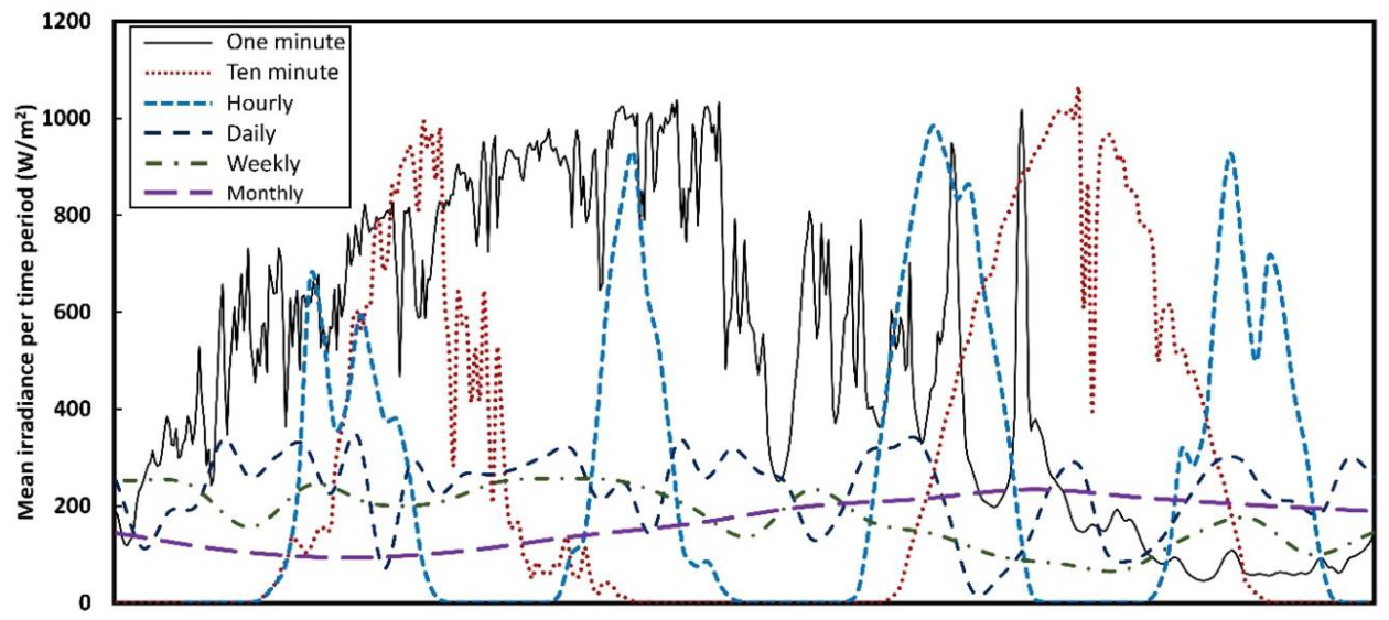
The variability of solar irradiance depends on the time scale. A single datum represents a mean value of more frequent measurement records for a given time period. For instance, an hourly value of GHI may be acquired from 60 pyranometer records at the one-minute interval. Therefore, a long time interval results in the smoothing effect, and thus the variability lessens. Figure 1 shows the smoothing effect on the solar irradiance variability. The data were recorded every minute at Kookmin University, South Korea and presented by different time scales. The finest temporal resolution of one minute reveals a high degree of variability, but the variability smooths out with the time scale. It should be noticed that the smoothing effect also appears when a spatial averaging over a large area is applied.
The variability of solar irradiance directly affects solar PV power systems’ performance and more seriously disturbs grid stability. The grid typically absorbs power fluctuations at short time scales as fluctuations in frequency and voltage. Therefore, grid operators can control the power ramp rate by imposing a limit on PV plants; for instance, 10% of the nameplate capacity per minute. In addition, grid operators need to balance supply and demand while complying with power system regulations. If the power supply exceeds demand, curtailment can be applied to disconnect power delivery from PV plants with the grid. Solar irradiance or PV power forecasting can optimize the ramp rate control and schedule the load-following operation more effectively with an energy storage system.
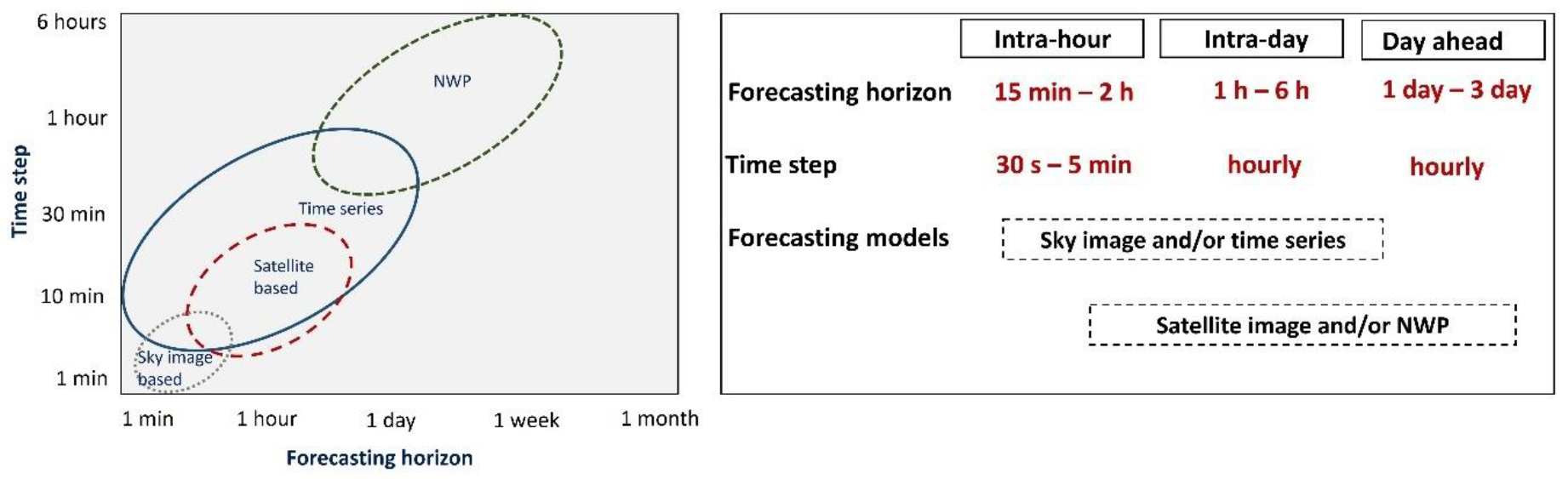
Various solar forecasting techniques have their own applicable regimes in terms of time scale. Thus, depending on solar irradiance variability of interest, an appropriate technique must be selected. Figure 2 illustrates a guideline to select forecasting techniques. For time horizons less than one hour, sky-image-based techniques offer very good forecasting capability [10]. Satellite-image-based techniques are recommended for several hours ahead of forecasting with a spatial resolution around 1–5 km [11]. Numerical weather predictions (NWP) allows long-term forecasting over 1 day and up to 15 days ahead, but its time step and update interval are large. On the other hand, time series forecasting using statistical models covers many applications from short to long terms with fine time steps [12,13,14]. As an advanced version of statistical models, deep learning models for sequential data are anticipated to expand the regime.
3. Deep Learning Models
This section provides an overview of the theoretical background of the selected deep learning models. We describe a neural network and activation function because they are fundamental for all types of neural network algorithms, although ANN is not in the scope of this review.
3.1. Neural Network
The neural network is inspired by the structure of the human brain and significantly contributed to machine learning technology development. It is a simplified mathematical model to solve various nonlinear problems. In the past, researchers reviewed ANN models in predicting solar energy, such as Yadav et al. [15] for solar radiation prediction, Mellit et al. [16] for PV applications, and Cheon et al. [17] for solar energy forecasting. One conclusion from these studies is that the ANN model predicts solar radiation more accurately than other conventional models, such as the Angstrom, conventional, linear, nonlinear, and fuzzy logic models.
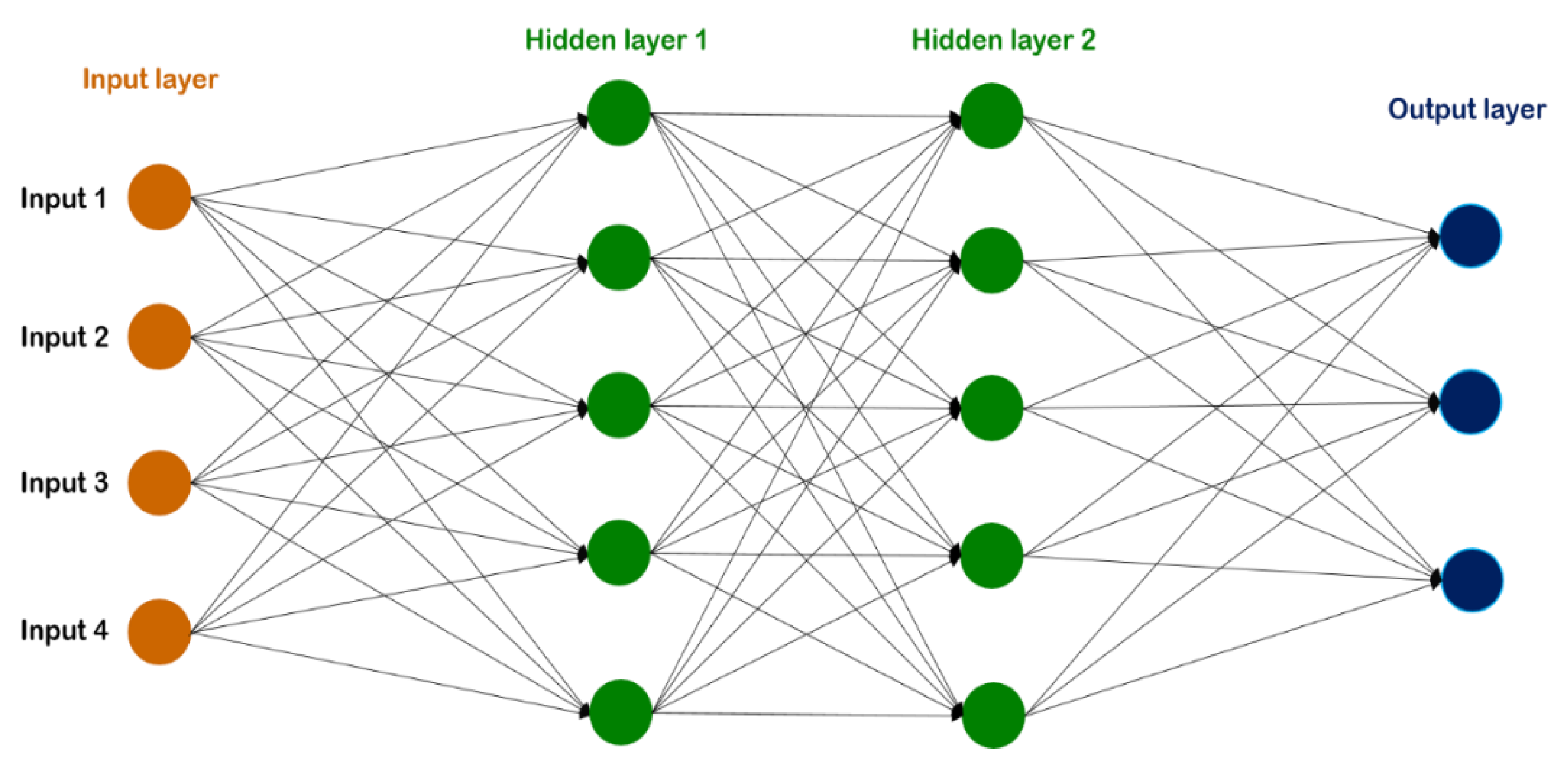
The neural network model comprises the input, hidden, and output layers with auxiliary components, such as neurons, weight, bias, and activation functions. Figure 3 shows the basic neural network architecture with a multilayer perceptron. The input layer receives input values, and the hidden layer analyzes the input values. The output layer collects the data from the hidden layer and decides the output. In the learning process, the neural network modifies its structure to get the same reference or set point as the supervisor. The training process will be repeated until the difference between the neural network output and the supervisor lies within an acceptable range [18].
The basic ANN mathematical formula can be expressed as
where An is the output, n is the number of input, wj is the weight, Ij is the input, and b is the bias.
The output value varies with the activation function. The activation function, also known as the transfer function, is a mathematical equation determining neurons’ output and can be divided into two types, namely, linear and nonlinear functions. A linear activation function generates the same linear result between the input and output layers. However, such a linear relationship is not enough for practical applications because the problems involve complex information and various parameters, such as image, video text, and sound. A neural network with a nonlinear activation function can tackle the limitations of the linear activation function. The commonly used activation functions are shown in Table 1. Note that the rectified linear unit (ReLU) and leaky ReLU are examples of nonlinear activation function because the slope is not constant for all values. Especially for ReLU, the slope is always either 0 for negative values or 1 for positive values.
3.2. RNN
RNNs are specially designed for analyzing sequential data and have been successfully used in fields such as speech recognition, machine translation, and image captioning [19]. RNN processes sequence data by elements and preserves a state to represent the information at time steps [20]. A traditional neural network assumes that all units of the input vectors are independent. Consequently, the traditional neural network is ineffective for predicting using sequential data.
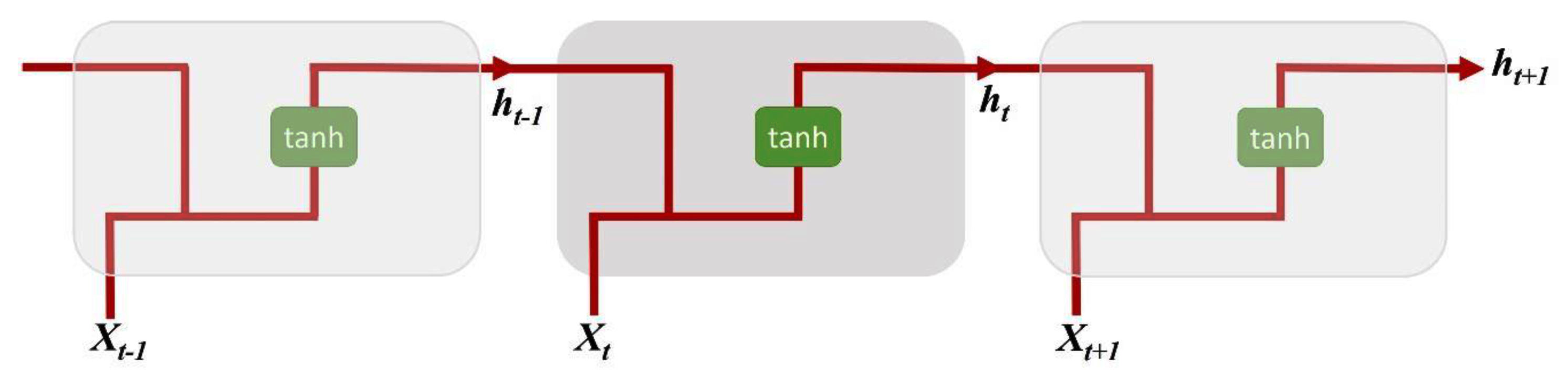
The architecture of RNN with three main components (input, hidden neuron, and activation function) is shown in Figure 4.
Previous hidden state (ht) can be formulated as
where xt is the input at time t, ht is the hidden neuron at time t, U is the weight of the hidden layer, and W is the transition weights of the hidden layer. The input and previous hidden states are combined to produce information as the current and previous input go through the tanh function. Then, the output is the new hidden state, performing as the neural network memory because it holds information from the previous network.
Training regular RNNs can be challenging because of vanishing and exploding gradient problems. In the case of the exploding gradient, the problem can be solved after the backpropagation is closed at a certain point. However, the result is not optimal because all the weights are not updated. In the case of the vanishing gradient, it can be fixed by initializing the weights to reduce the possibility of vanishing gradient. However, an alternative treatment to solve the problem is to use LSTM, which we discuss later.
3.3. LSTM
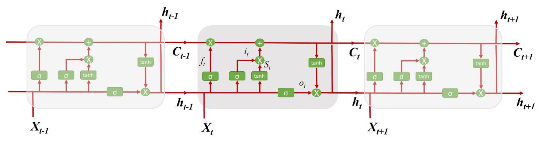
LSTM is a time RNN proposed by Hochreiter et al. [21] to learn the long-term dependence of information. An LSTM has a similar flow as an RNN. The difference is the operation inside the cells. An LSTM unit comprises forget, input, and output gates (Figure 5). The forget gate categorizes the information that should be thrown away or kept. The input gate updated the cells, and the output gate decides the next hidden state. Furthermore, LSTM has an internal memory unit and gate mechanism to overcome both the vanishing gradient and explosion gradient problems in the training process of RNN [22].
The mathematical symbols in the above equations are as follows:
- Xt is the input vector to the memory cell at time t.
- Wi, Wf, Wc, Wo, Ui, Uf, Uc, Uo, and Vo are weight matrices.
- bi, bf, bc, and bo are bias vectors.
- ht is the value of the memory cell at time t.
- St and Ct are the values of the candidate state of the memory cell and the state of the memory cell at time t, respectively.
- σ and tanh are the activation functions.
- it, ft, and ot are values of the input gate, the forget gate, and the output gate at time t.
The forget gate (ft), input gate (it), and output gate (ot) in Equations (3), (4) and (7) have values from 0 to 1 through the sigmoid function (σ). A value of one means that all input information passes through the gate, but a value of 0 shows that no input information passes [23]. The values of the candidate state of the memory cells in Equation (6) calculate the new information at time t, and its output through the tanh function has a value between −1 and 1. The state of the memory at the cell, controlled by the forget and input gates, is calculated as variable Ct of time t (Equation (7)). The selected values are converted into output by multiplying them by ot and output becomes ht (Equation (8)).
3.4. GRU
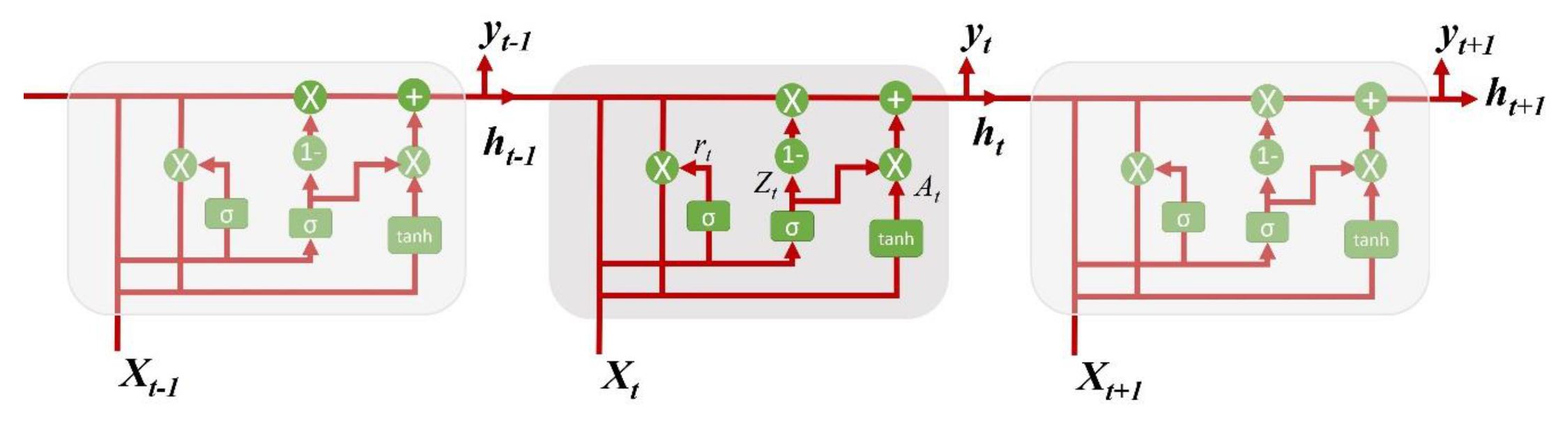
Cho et al. [24] first proposed GRU as a simpler RNN architecture than LSTM, resulting in easier computation and implementation. GRU is similar to LSTM in terms of remembering valuable information and capturing long-term dependencies. The strength of GRU is that the computational time is more efficient with less complexity because of fewer parameters than LSTM [25]. GRU also only has two gates, namely, a reset and an update gate. The update gate is the same as the forget and input gate in LSTM because it selects what information should be stored or erased. Meanwhile, the reset gate decides the amount of information that must be forgotten. Therefore, the training time of GRU is faster than LSTM.
The structure of GRU is shown in Figure 6, and the relationship between the input and output for GRU can be written as:
where rt is the reset gate, Zt is the update gate, At is the memory content, σ and tanh are the activation functions, and ht is the final memory at the current time step. The reset (rt) and update gate (Zt) have values from 0 to 1 through the sigmoid function (σ) in Equations (9) and (10). Meanwhile, the memory content (At), using the rest gate to store the relevant information from the past, has a value between −1 and 1 through tanh.
3.5. The Hybrid Model (CNN–LSTM)
CNN is a deep learning algorithm by considering spatial inputs. Identical to other neural networks, CNN neurons have learnable weights and biases. However, CNN is mainly used for processing data with a grid topology, giving it a specific characteristic of its architecture [26].
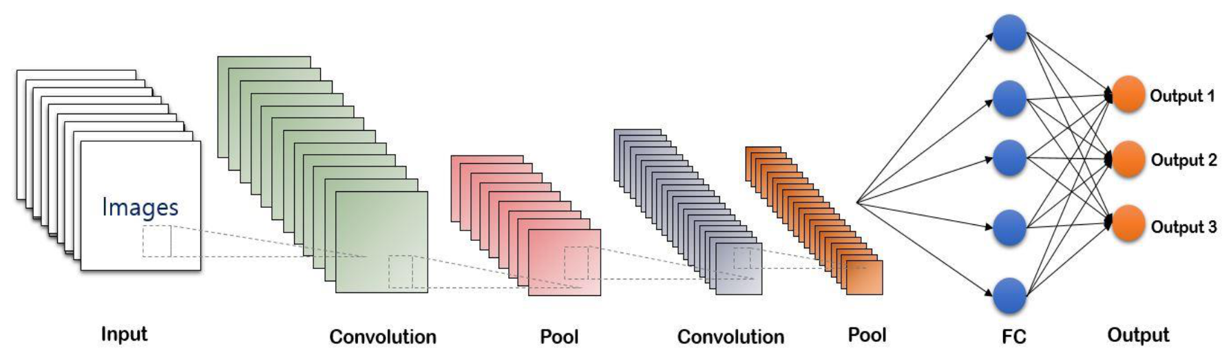
CNN is a feedforward network because information flow occurs in one direction only, that is, from their inputs to their outputs [27]. The CNN model uses three main layers, namely, the convolutional, pooling, and fully connected layers (Figure 7). The convolutional and pooling layers are used to reduce the computational complexity. Meanwhile, the fully connected layer is the flattened layer connected to the output. Various pooling techniques are available in the architecture of CNN. However, max pooling is mostly used in CNN layers, where the pooling window contains the maximum value from each element [28].
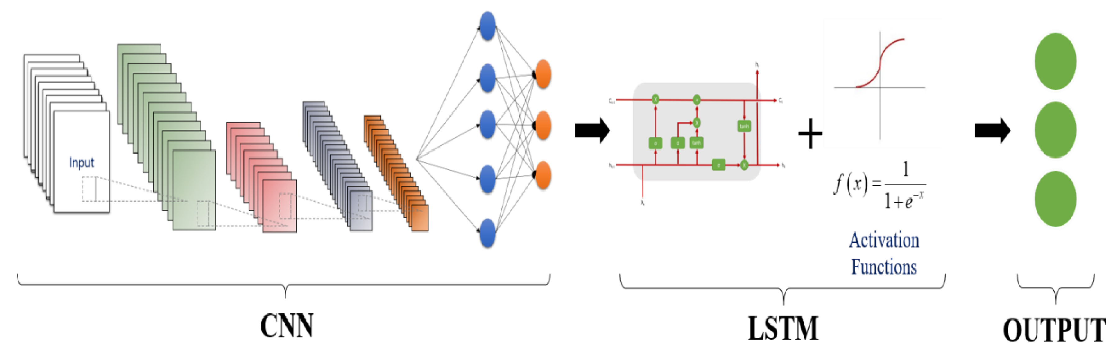
CNN–LSTM was developed for visual time series prediction problems and generating textual descriptions from the sequences of images. The CNN–LSTM architecture uses CNN layers for feature extraction on input data and combines with LSTM to support sequence prediction. Specifically, CNN extracts the features from spatial inputs and uses them in the LSTM architecture to output the caption. The architecture of the CNN–LSTM model is illustrated in Figure 8.
The applications of this hybrid model have been used to solve many problems, such as rod pumping [29], particulate matter [30], waterworks [31], and heart rate signals [32]. Studies have demonstrated promising results; for example, Xingjian et al. [33] predicted the future rainfall intensity in a local region over a relatively short period. The experiments show that the CNN–LSTM network captures spatiotemporal correlations better and consistently outperforms the fully connected LSTM (FC-LSTM) model for precipitation forecasting.
4. Evaluation Metrics
Evaluation metrics are critical for explaining the forecast performance of deep learning models [34]. The metrics provide feedback regarding the accuracy of the forecasting to improve the models until a desirable accuracy is achieved. Various evaluation metrics are available for calculating the accuracy of prediction. The typical evaluation metrics for solar irradiance and PV power forecasting are summarized in Table 2. Here, Ppred, Pmeas, and n represent the forecasted values at each time, the measured values at each time, and the number of sample data for the period, respectively.
Mean absolute error (MAE) measures the average magnitude of error in a set of predictions using the absolute value. If the absolute sign is removed, the evaluation metric becomes MBE, capturing the average bias in the prediction, such that positive and negative values represent overprediction and underprediction, respectively. However, root-mean-square error evaluation metric (RMSE) measures the deviation from the measurement, and thus, the smaller, the better. When mean values vary with location or system, a direct comparison of evaluation metrics could lead to a misunderstanding. In such cases, the percentage or relative metrics such as Mean absolute percentage error (MAPE) and relative root-mean-square error (rRMSE) are more useful. Forecasting skill measures the forecasting model over the persistence model regarding RMSE, where the persistence model assumes that the atmospheric conditions are stationary. A positive forecasting skill value means that the model is outperforming the persistence model. Note that measurement data include uncertainty by nature, and thus, the true values are unknown. Hence, researchers prefer to use differences, such as root-mean-square difference (rRMSD) and relative mean bias difference (rMBD) [35].
5. Analysis of Past Studies
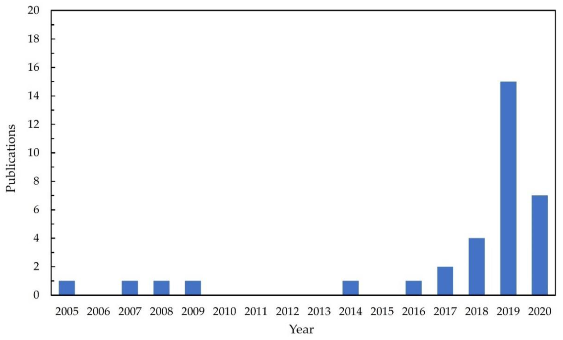
In this section, we present notable findings in forecasting solar irradiance and PV power after analyzing the published studies based on RNN, LSTM, GRU, and CNN–LSTM hybrid models. In total, 35 papers from 2005 to 2020 were collected and plotted by the publication year (Figure 9). From 2005 to 2017, only a few papers were published because these deep learning models were unpopular then. However, the number of publications increased dramatically since 2018. The number of publications grew by 250%, from 4 in 2018 to 14 in 2019. Meanwhile, only the publications until early 2020 were collected, and more publications are expected by the end of the year.
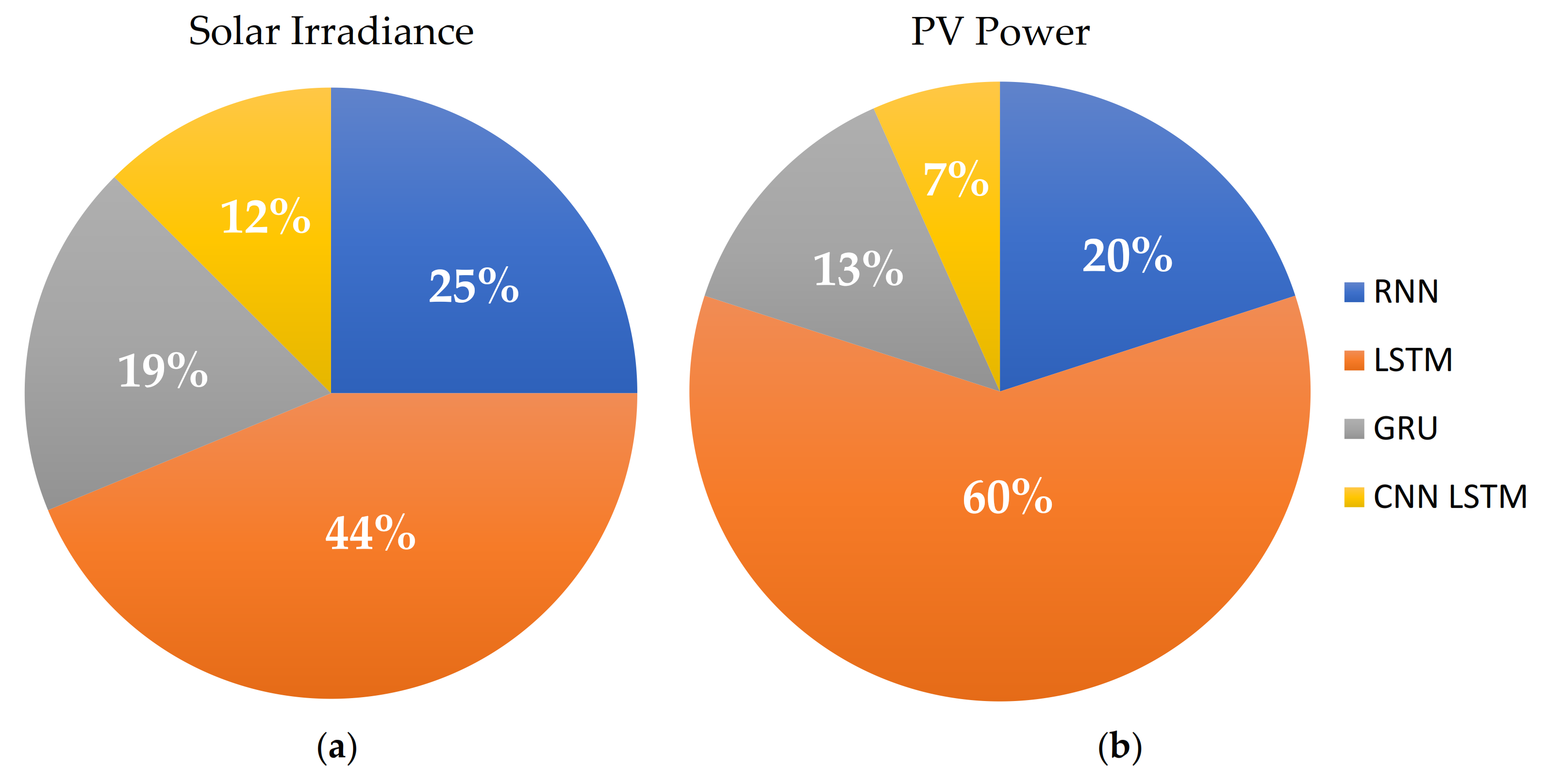
The proportion of publications by deep learning models for predicting solar irradiance and PV power individually is shown in Figure 10. In both cases, the LSTM accounts for most publications, with RNN and GRU following. Meanwhile, the CNN–LSTM hybrid model shows the lowest contribution. The popularity of the LSTM model is higher than that of the other standalone models because it provides promising accuracy in the case of solar energy forecasting. The CNN–LSTM also has a better performance than other models. However, the percentage of publications using this model is smaller than using other models because the CNN–LSTM is a new solar energy forecasting model.
It should be noted that we did an independent review for solar irradiance and PV power because the units and range values are different. Solar irradiance refers to the amount of solar radiation per unit area; meanwhile, PV power refers to the use of solar radiation as thermal energy through PV cells in the solar panel. The total solar radiation on the earth’s atmosphere is approximately 1360 W/m2, called the solar constant. This value is attenuated to the earth’s surface through a complex series of reflections, absorptions, and remissions. Solar irradiance fluctuates because it is affected by several factors such as atmosphere condition, geographic location, season, and time of day. Although the amount of power generated by PV at a particular location depends on how much of the solar irradiance reaches it, the PV power output also relies on the solar panel’s size and efficiency. Therefore, it is essential to describe the specification of the solar panel for getting accurate PV output information.
5.1. Accuracy
The prediction accuracy is the most critical factor in selecting a forecast model. We chose RMSE as the basic evaluation metric because it is most popular in solar energy forecasting. Because the mean value of solar irradiance or PV power differs by factors such as location and system size, rRMSE is a better measure to compare the accuracy between studies. Unfortunately, only a few studies presented rRMSE. We selected the best accuracy out of all the studied cases. Table 3 and Table 4 list the accuracy of the papers, including forecast horizon, time interval, input parameters, and the size of PV systems in the case of PV forecasting.
Regarding solar irradiance forecasting in Table 3, the forecast horizon ranges from 5 min to 1 day ahead. Meanwhile, the time interval data vary from every 5 min to 1 h. Generally, the CNN–LSTM as the hybrid model performs better to predict solar irradiance for one day-ahead forecasting. Ghimire et al. [36] have the best performances of all the studies with RMSE values of 8.189 W/m2. For LSTM and GRU, the best performance was the prediction of solar irradiance for 10 min ahead at 5 min intervals. However, RNN tends to result in lower accuracy than other models for day-ahead hourly forecasting.
In this case, the main factor causing changes in solar irradiation is the presence of clouds. Unfortunately, only some studies explained the condition of the sky. For example, Wang et al. [25] demonstrated that the CNN–LSTM hybrid outperformed the single LSTM to predict one day-ahead solar irradiation at 15 min intervals on sunny days, showing the small error where the RMSE value is less than 34 W/m2. Meanwhile, Niu et al. [37] have the largest error in forecasting solar irradiance using the RNN model where the RMSE value is 195 W/m2; however, the sky conditions are not mentioned in the present study. Hence, further study regarding deep learning models to predict solar irradiance is required to create a concrete solution.
The performances for PV power forecasting are listed in Table 4. Most publications focused on predicting PV power in intra-hour forecast horizons. The RMSE reveals a wide variation from 0.044 to 15,290 kW because PV power generation is proportional to system size. Accuracy comparison is more difficult in PV power forecasting than in solar irradiance forecasting, suggesting an increasing need for evaluation based on rRMSE. For the LSTM models in references (Zhang et al. [46]; Wang et al. [47]; Li et al. [48]), the RMSE value increases as the PV size increases. The values are 0.139, 0.398, and 0.885 kW for the PV size of 60.00, 153.48, and 199.16 m2, respectively.
5.2. Types of Input Data
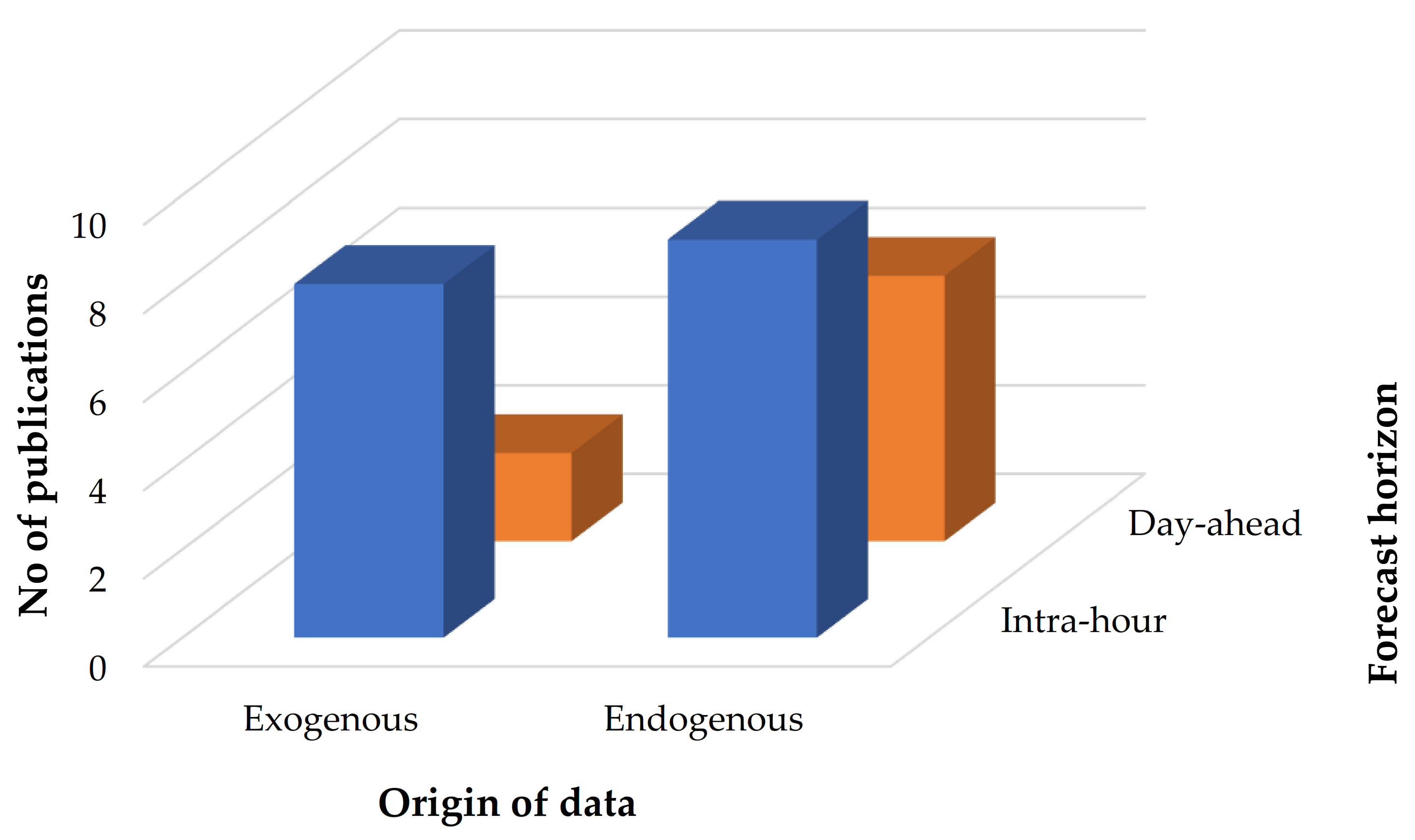
The type of input data, endogenous and exogenous, can classify forecasting models. In the endogenous model, the type of input and output data is identical. That is, historical PV power data are used for forecasting future PV power. However, the exogenous model uses other data types, such as ambient temperature, humidity, wind speed, wind direction, and sun position, besides the type of output data. It should be noted that the cited references used historical data prediction as input rather than numerical weather prediction data. The time period of input data is also summarized in Table 3 and Table 4. The number of publications by exogenous and endogenous inputs, and the forecast horizon is illustrated in Figure 11. For the intra-hour and day-ahead forecast horizons, the endogenous model outnumbers the exogenous model.
Li et al. [55] presented RNN and LSTM models using endogenous inputs for predicting PV power output in the very short term. They used both PV power data from the previous day and previous forecasting data as the input. The results demonstrated that the average RMSE, MAPE, and MAE outperform the other models such as SVM, radial basis function (RBF), back propagation neural network (BPNN), and persistence in the 15 and 30 min forecasting horizons.
Husein et al. [3] proposed an LSTM model using exogenous inputs to forecast day-ahead solar irradiance. The models used dry bulb temperature, dewpoint temperature, and relative humidity as input from six locations. The results showed that LSTM outperforms the feedforward neural network (FFNN) for data from all locations. They also simulated a one-year operation of a commercial building microgrid using the actual and forecasted solar irradiance, and the results showed that using the forecasting approach increases the annual energy savings by 2% compared with FFNN.
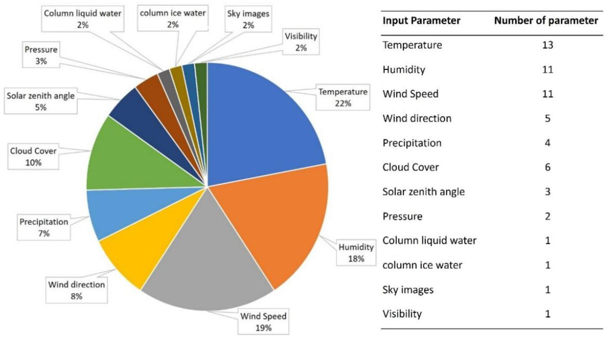
We investigated the exogenous input parameters from 25 publications (Figure 12). The less frequently used parameters include visibility, sky images, column ice water, column liquid water, and pressure. However, it shows that temperature, humidity, and wind speed are used more frequently because they are easier to collect than other parameters.
The period of historical data also affects the performance of the prediction. If the time series is too short, it will lead to a lack of information for learning, and if the time series is too long, it will increase the complexity of the algorithm. However, the increase in time series data does not guarantee better performance. Wang et al. [47] compared the errors of the LSTM and CNN–LSTM according to input sequences (Table 5). The results show that errors increase from 0.5 to 2 years of input time series data. The best accuracy was observed when three years of input sequences were used. Historical data of more than three years degraded performances, implying that the period of input data must be optimized.
5.3. Forecast Horizon
The forecast horizon is the length of time into the future for which a model can predict, and it strongly influences the performances and characteristics of the forecast. Forecasting horizons can be divided into four types [59]:
- Very short-term forecasting (1 min to several minutes ahead).
- Short-term forecasting (1 h or several hours ahead to 1 day or 1 week ahead).
- Medium-term forecasting (1 month to 1 year ahead).
- Long-term forecasting (1 to 10 years ahead).
Yan et al. [45] studied LSTM and GRU’s performance to predict solar irradiance for very short-term forecasting. The experiments were conducted in time ranges of 5, 10, 20, and 30 min and the four seasons. The RMSE in Table 6 shows that LSTM and GRU’s smallest error occurred in winter for the 10 min forecast horizon. Generally, the two models showed a gradual increase of errors for the 10 to 30 min solar irradiance forecasting.
Ghimire et al. [36] used the CNN–LSTM hybrid model and three standalone models for solar irradiance forecasting. The forecasting errors for those models are listed in Table 7. CNN–LSTM was used using 30 min interval data to predict solar irradiance for a 1 day up to 1-month forecast horizon, as measured by RMSE and MAE. Compared with RNN, LSTM, and GRU, the hybrid model outperforms other models to predict solar irradiance in all forecasting horizons.
5.4. Type of Season and Weather
The accuracy of deep learning models has been proven for the different seasons and types of weather. For example, Li et al. [48] used RNN, LSTM, and GRU models for short-term PV power forecasting. The performance evaluations of the different models for each season and types of weather are presented in Table 8. Except for winter, generally, the LSTM model outperforms the two other models. In winter, the GRU model is better than LSTM and RNN for all types of weather.
5.5. Training Time
Deep learning with many parameters requires distributed training, where training time is critical [60]. Training time is the product of the deep learning models that must be performed to reach the desired level of accuracy. Each deep learning model has a different training time to reach the best performance. Hence, in this section, we compared the training time for each model to know which model is more efficient in forecasting solar irradiation and PV power.
Wang et al. [25] conducted forecasting experiments for LSTM and GRU to experience information training time in the best, worst, and average cases. LSTM and GRU’s training times in the three cases are presented in Table 9, proving that GRU is better than LSTM because the longest training time of GRU is shorter than the best training time of the LSTM.
The training times of LSTM and GRU in Seoul and Busan in 2016 and 2017 are shown in Table 10. Aslam et al. [40] measured LSTM and GRU’s performance as training time in a system with an AMD Ryzen Thread ripper 2950X and 64 GB RAM. The mean values taken from 10 runs for accurate results were taken. GRU performed faster than LSTM in hourly and daily forecasting. For hourly prediction, the difference in training time is more than 200 s, and for daily forecasting, it is less than 20 s in each year and region.
5.6. Comparison with Other Models
In this section, RNN, LSTM, GRU, and CNN–LSTM are compared in Table 11, Table 12, Table 13, Table 14 and Table 15 with other machine learning models and deep learning models. Pang et al. [61] proposed a hierarchical approach to predict solar irradiance using ANN and RNN in Tuscaloosa, Alabama, USA. The data from 22 to 28 May 2016 were used to predict solar irradiance into three interval times (10, 30, and 60 min) (Table 12). Consequently, RNN outperformed ANN in forecasting horizon data sampling, and the best result for the forecast horizon is when the shortest horizon was considered.
In the case of LSTM, Alzahrani et al. [62] studied a machine learning approach in Chicago, USA, where the study compared various prediction models on a test dataset using FFNN and support vector regression (SVR). The data were collected over four days (24 March, 8 February, 8 October, and 12 August) and split into three parts, namely, data training, data testing, and data validation in portions of 70%, 15%, and 15%, respectively. The results in Table 13 show that LSTM has a better performance in achieving an RMSE of 0.086 W/m2, whereas FFNN and SVR obtained 0.160 and 0.110 W/m2, respectively.
Lee et al. [63] compared CNN–LSTM, random forest regression (RFR), and SVR. They considered two sets of inputs: a PV measurement incorporated with weather values from a nearby meteorological station and only past PV measurements. They collected 18,620 hourly data time series and divided the data training and data testing as 75% and 25%, respectively. The results in the first case show that CNN–LSTM has the lowest error metrics with an RMSE of 0.098 kW. However, the excluded weather data case shows that SVR is better than RFR and CNN–LSTM with 0.126 kW (Table 14).
Li et al. [48] presented their results for the comparison between GRU and multilayer perceptron (MLP) in a different season (Table 15). They collected the data in DKASC, Alice Springs, Australia. The generation of the PV system is 26.500 kW. In this case, they used the data from 1 June 2014 to 31 May 2015, as the training dataset, and the data for 12 June 2016, were used as the testing dataset. The results show that MLP has a better performance than GRU only in the autumn, with a value of 1061 kW. However, the average value of GRU has the most representative attributes of all the seasons compared with MLP.
6. Conclusions
This paper introduced deep learning models as techniques to predict solar irradiance and PV power generation. To represent a complete review of the models, the evaluation for the PV power and solar irradiance forecasting is made apart. The main reason because the output is different in terms of function, unit, and range value. Although the value fluctuates because it is affected by several factors such as atmosphere condition, geographic location, season, and time of day, the evaluation of solar irradiance forecasting is uncomplicated to understand. Radiation from the sun that reaches the earth’s surface is measured in power per unit area; hence it is possible to compare the solar irradiance at different locations. However, apart from the main factors, the PV power output relies on the solar panel’s size and efficiency. Therefore, in part of the review of PV power forecasting, the solar panel size is described to obtain accurate PV output information.
RNN, LSTM, GRU, and CNN–LSTM have become the topics of research interest because of their popularity in predicting solar energy. They also offer many advantages over other machine learning models, especially regarding time series data forecasting. Each model has its strengths and limitations to predict solar irradiance and PV power; therefore, it is challenging to decide which is the best among all the models. However, from the studies reviewed in this paper, we propose the following conclusions:
- In the case of the single model, most studies explain that LSTM and GRU show better performance than RNN in all conditions because LSTM and GRU have internal memory to overcome the vanishing gradient problems occurring in the RNN.
- The hybrid model (CNN–LSTM) outperforms the three standalone models in predicting solar irradiance. More specifically, the evaluation metrics for this hybrid model are substantially smaller than those of the standalone models. However, the CNN–LSTM model requires complex input data, such as images, because it has a CNN layer inside.
- The training time should be considered to recognize the performance of the models. This work reveals that the statistics of GRU are more efficient than that of LSTM in the case of computational time because the average time for LSTM to train the data is relatively longer than that for GRU. Therefore, considering training time and forecasting accuracy, the GRU model can generate a satisfactory result for forecasting PV power and solar irradiance.
- Comparisons between the deep learning models and other machine learning models conclude that these models were better used in predicting solar irradiance and PV power (Section 5.6). Most studies show that the accuracy of the proposed models is better than other models, such as ANN, FFNN, SVR, RFR, and MLP.
Author Contributions
R.A.R.: conceptualization, methodology, formal analysis, writing—original draft; R.A.A.R.: conceptualization, investigation; H.-J.L.: writing—review and editing, supervision, funding acquisition. All authors have read and agreed to the published version of the manuscript.
Funding
The present study is financially supported by grants from the National Research Foundation of Korea (NRF), Ministry of Science and ICT (2018M1A3A3A02065823, 2019R1A2C1009501).
Conflicts of Interest
The authors declare no conflict of interest.
Abbreviation
| ANN | Artificial neural network |
| BPNN | Back propagation neural network |
| CNN | Convolutional neural network |
| DHI | Diffuse horizontal irradiance |
| FFNN | Feedforward neural network |
| GHI | Global horizontal irradiance |
| GRU | Gated recurrent unit |
| LSTM | Long short-term memory |
| MAE | Mean absolute error |
| MAPE | Mean absolute percentage error |
| MLP | Multilayer perceptron |
| PV | Photovoltaic |
| RBF | Radial basis function |
| ReLU | Rectified linear unit |
| RFR | Random forest regression |
| RMSE | Root-mean-square error |
| RNN | Recurrent neural network |
| rRMSE | Relative root-mean-square error |
| SVR | Support vector regression |
References
- Mohanty, S.; Patra, P.K.; Sahoo, S.S.; Mohanty, A. Forecasting of solar energy with application for a growing economy like India: Survey and implication. Renew. Sustain. Energy Rev. 2017, 78, 539–553. [Google Scholar] [CrossRef]
- Das, U.K.; Tey, K.S.; Seyedmahmoudian, M.; Mekhilef, S.; Idris, M.Y.I.; Van Deventer, W.; Horan, B.; Stojcevski, A. Forecasting of photovoltaic power generation and model optimization: A review. Renew. Sustain. Energy Rev. 2018, 81, 912–928. [Google Scholar] [CrossRef]
- Husein, M.; Chung, I.-Y. Day-Ahead Solar Irradiance Forecasting for Microgrids Using a Long Short-Term Memory Recurrent Neural Network: A Deep Learning Approach. Energies 2019, 12, 1856. [Google Scholar] [CrossRef] [Green Version]
- Lappalainen, K.; Wang, G.C.; Kleisslid, J. Estimation of the largest expected photovoltaic power ramp rates. Appl. Energy 2020, 278, 115636. [Google Scholar] [CrossRef]
- Sobri, S.; Koohi-Kamali, S.; Rahim, N.A. Solar photovoltaic generation forecasting methods: A review. Energy Convers. Manag. 2018, 156, 459–497. [Google Scholar] [CrossRef]
- Ng, A. Machine Learning Yearning: Techincal Strategy for AI Engineers, in the Era of Deep Learning. 2018. Available online: https://www.deeplearning.ai/machine-learning-yearning (accessed on 30 November 2020).
- Zang, H.; Liu, L.; Sun, L.; Cheng, L.; Wei, Z.; Sun, G. Short-term global horizontal irradiance forecasting based on a hybrid CNN-LSTM model with spatiotemporal correlations. Renew. Energy 2020, 160, 26–41. [Google Scholar] [CrossRef]
- Shuai, Y.; Notton, G.; Kalogirou, S.; Nivet, M.-L.; Paoli, C.; Motte, F.; Fouilloy, A. Machine learning methods for solar radiation forecasting: A review. Renew. Energy 2017, 105, 569–582. [Google Scholar] [CrossRef]
- Carrera, B.; Kim, K. Comparison Analysis of Machine Learning Techniques for Photovoltaic Prediction Using Weather Sensor Data. Sensors 2020, 20, 3129. [Google Scholar] [CrossRef]
- Caldas, M.; Alonso-Suárez, R. Very short-term solar irradiance forecast using all-sky imaging and real-time irradiance measurements. Renew. Energy 2019, 143, 1643–1658. [Google Scholar] [CrossRef]
- Miller, S.D.; Rogers, M.A.; Haynes, J.M.; Sengupta, M.; Heidinger, A.K. Short-term solar irradiance forecasting via satellite/model coupling. Sol. Energy 2018, 168, 102–117. [Google Scholar] [CrossRef]
- Xie, T.; Zhang, G.; Liu, H.; Liu, F.; Du, P. A Hybrid Forecasting Method for Solar Output Power Based on Variational Mode Decomposition, Deep Belief Networks and Auto-Regressive Moving Average. Appl. Sci. 2018, 8, 1901. [Google Scholar] [CrossRef] [Green Version]
- Wang, K.; Li, K.; Zhou, L.; Hu, Y.; Cheng, Z.; Liu, J.; Chen, C. Multiple convolutional neural networks for multivariate time series prediction. Neurocomputing 2019, 360, 107–119. [Google Scholar] [CrossRef]
- Chaouachi, A.; Kamel, R.M.; Nagasaka, K. Neural Network Ensemble-Based Solar Power Generation Short-Term Forecasting. J. Adv. Comput. Intell. Intell. Inform. 2010, 14, 69–75. [Google Scholar] [CrossRef] [Green Version]
- Yadav, A.K.; Chandel, S. Solar radiation prediction using Artificial Neural Network techniques: A review. Renew. Sustain. Energy Rev. 2014, 33, 772–781. [Google Scholar] [CrossRef]
- Mellit, A.; Kalogirou, S.A. Artificial intelligence techniques for photovoltaic applications: A review. Prog. Energy Combust. Sci. 2008, 34, 574–632. [Google Scholar] [CrossRef]
- Cheon, J.; Lee, J.T.; Kim, H.G.; Kang, Y.H.; Yun, C.Y.; Kim, C.K.; Kim, B.Y.; Kim, J.Y.; Park, Y.Y.; Jo, H.N.; et al. Trend Review of Solar Energy Forecasting Technique. J. Korean Sol. Energy Soc. 2019, 39, 41–54. [Google Scholar] [CrossRef]
- Hameed, W.I.; Sawadi, B.A.; Al-Kamil, S.J.; Al-Radhi, M.S.; Al-Yasir, Y.I.; Saleh, A.L.; Abd-Alhameed, R.A. Prediction of Solar Irradiance Based on Artificial Neural Networks. Inventions 2019, 4, 45. [Google Scholar] [CrossRef] [Green Version]
- Fan, C.; Wang, J.; Gang, W.; Li, S. Assessment of deep recurrent neural network-based strategies for short-term building energy predictions. Appl. Energy 2019, 236, 700–710. [Google Scholar] [CrossRef]
- Chollet, F.; Allaire, J. Deep Learning with R; Manning Publications: Shelter Island, NY, USA, 2018. [Google Scholar]
- Hochreiter, S.; Schmidhuber, J. Long Short-Term Memory. Neural Comput. 1997, 9, 1735–1780. [Google Scholar] [CrossRef]
- Liu, Y.; Guan, L.; Hou, C.; Han, H.; Liu, Z.; Sun, Y.; Zheng, M. Wind Power Short-Term Prediction Based on LSTM and Discrete Wavelet Transform. Appl. Sci. 2019, 9, 1108. [Google Scholar] [CrossRef] [Green Version]
- Kim, H.Y.; Won, C.H. Forecasting the volatility of stock price index: A hybrid model integrating LSTM with multiple GARCH-type models. Expert Syst. Appl. 2018, 103, 25–37. [Google Scholar] [CrossRef]
- Cho, K.; Van Merrienboer, B.; Gulcehre, C.; Bahdanau, D.; Bougares, F.; Schwenk, H.; Bengio, Y. Learning phrase representations using RNN encoder-decoder for statistical machine translation. In Proceedings of the 2014 Conference on Empirical Methods in Natural Language Processing (EMNLP), Doha, Qatar, 14–21 October 2014; pp. 1724–1734. [Google Scholar] [CrossRef]
- Wang, F.; Yu, Y.; Zhang, Z.; Li, J.; Zhen, Z.; Li, K. Wavelet Decomposition and Convolutional LSTM Networks Based Improved Deep Learning Model for Solar Irradiance Forecasting. Appl. Sci. 2018, 8, 1286. [Google Scholar] [CrossRef] [Green Version]
- Yann, L.; Yoshua, B. Convolutional Networks for Images, Speech, and Time-Series. Handb. Brain Theory Neural Netw. 1995, 10, 2571–2575. [Google Scholar]
- Rawat, W.; Wang, Z. Deep Convolutional Neural Networks for Image Classification: A Comprehensive Review. Neural Comput. 2017, 29, 2352–2449. [Google Scholar] [CrossRef]
- Rehman, A.U.; Malik, A.K.; Raza, B.; Ali, W. A Hybrid CNN-LSTM Model for Improving Accuracy of Movie Reviews Sentiment Analysis. Multimed. Tools Appl. 2019, 78, 26597–26613. [Google Scholar] [CrossRef]
- He, Y.; Liu, Y.; Shao, S.; Zhao, X.; Liu, G.; Kong, X.; Liu, L. Application of CNN-LSTM in Gradual Changing Fault Diagnosis of Rod Pumping System. Math. Probl. Eng. 2019, 2019, 4203821. [Google Scholar] [CrossRef]
- Huang, C.-J.; Kuo, P.-H. A Deep CNN-LSTM Model for Particulate Matter (PM2.5) Forecasting in Smart Cities. Sensors 2018, 18, 2220. [Google Scholar] [CrossRef] [Green Version]
- Cao, K.; Kim, H.; Hwang, C.; Jung, H. CNN-LSTM coupled model for prediction of waterworks operation data. J. Inf. Process. Syst. 2018, 14, 1508–1520. [Google Scholar] [CrossRef]
- Swapna, G.; Soman, K.P.; Vinayakumar, R. Automated detection of diabetes using CNN and CNN-LSTM network and heart rate signals. Procedia Comput. Sci. 2018, 132, 1253–1262. [Google Scholar] [CrossRef]
- Shi, X.; Chen, Z.; Wang, H.; Yeung, D.Y.; Wong, W.K.; Woo, W.C. Convolutional LSTM network: A machine learning approach for precipitation nowcasting. Adv. Neural Inf. Process. Syst. 2015, 2015, 802–810. [Google Scholar]
- Zhang, J.; Florita, A.; Hodge, B.-M.; Lu, S.; Hamann, H.F.; Banunarayanan, V.; Brockway, A.M. A suite of metrics for assessing the performance of solar power forecasting. Sol. Energy 2015, 111, 157–175. [Google Scholar] [CrossRef] [Green Version]
- Lave, M.; Hayes, W.; Pohl, A.; Hansen, C.W. Evaluation of Global Horizontal Irradiance to Plane-of-Array Irradiance Models at Locations across the United States. IEEE J. Photovolt. 2015, 5, 597–606. [Google Scholar] [CrossRef]
- Ghimire, S.; Deo, R.C.; Raj, N.; Mi, J. Deep solar radiation forecasting with convolutional neural network and long short-term memory network algorithms. Appl. Energy 2019, 253, 113541. [Google Scholar] [CrossRef]
- Niu, F.; O’Neill, Z. Recurrent Neural Network based Deep Learning for Solar Radiation Prediction. In Proceedings of the 15th IBPSA Conference, San Francisco, CA, USA, 7–9 August 2017; pp. 1890–1897. [Google Scholar]
- Cao, S.; Cao, J. Forecast of solar irradiance using recurrent neural networks combined with wavelet analysis. Appl. Therm. Eng. 2005, 25, 161–172. [Google Scholar] [CrossRef]
- Qing, X.; Niu, Y. Hourly day-ahead solar irradiance prediction using weather forecasts by LSTM. Energy 2018, 148, 461–468. [Google Scholar] [CrossRef]
- Aslam, M.; Lee, J.-M.; Kim, H.-S.; Lee, S.-J.; Hong, S. Deep Learning Models for Long-Term Solar Radiation Forecasting Considering Microgrid Installation: A Comparative Study. Energies 2019, 13, 147. [Google Scholar] [CrossRef] [Green Version]
- He, H.; Lu, N.; Jie, Y.; Chen, B.; Jiao, R. Probabilistic solar irradiance forecasting via a deep learning-based hybrid approach. IEEJ Trans. Electr. Electron. Eng. 2020, 15, 1604–1612. [Google Scholar] [CrossRef]
- Jeon, B.-K.; Kim, E.-J. Next-Day Prediction of Hourly Solar Irradiance Using Local Weather Forecasts and LSTM Trained with Non-Local Data. Energies 2020, 13, 5258. [Google Scholar] [CrossRef]
- Wojtkiewicz, J.; Hosseini, M.; Gottumukkala, R.; Chambers, T. Hour-Ahead Solar Irradiance Forecasting Using Multivariate Gated Recurrent Units. Energies 2019, 12, 4055. [Google Scholar] [CrossRef] [Green Version]
- Yu, Y.; Cao, J.; Zhu, J. An LSTM Short-Term Solar Irradiance Forecasting Under Complicated Weather Conditions. IEEE Access 2019, 7, 145651–145666. [Google Scholar] [CrossRef]
- Yan, K.; Shen, H.; Wang, L.; Zhou, H.; Xu, M.; Mo, Y. Short-Term Solar Irradiance Forecasting Based on a Hybrid Deep Learning Methodology. Information 2020, 11, 32. [Google Scholar] [CrossRef] [Green Version]
- Zhang, J.; Verschae, R.; Nobuhara, S.; LaLonde, J.-F. Deep photovoltaic nowcasting. Sol. Energy 2018, 176, 267–276. [Google Scholar] [CrossRef] [Green Version]
- Wang, K.; Qi, X.; Liu, H. Photovoltaic power forecasting based LSTM-Convolutional Network. Energy 2019, 189, 116225. [Google Scholar] [CrossRef]
- Li, P.; Zhou, K.; Lu, X.; Yang, S. A hybrid deep learning model for short-term PV power forecasting. Appl. Energy 2020, 259, 114216. [Google Scholar] [CrossRef]
- Suresh, V.; Janik, P.; Rezmer, J.; Leonowicz, Z. Forecasting Solar PV Output Using Convolutional Neural Networks with a Sliding Window Algorithm. Energies 2020, 13, 723. [Google Scholar] [CrossRef] [Green Version]
- Gensler, A.; Henze, J.; Sick, B.; Raabe, N. Deep Learning for solar power forecasting—An approach using AutoEncoder and LSTM Neural Networks. In Proceedings of the 2016 IEEE International Conference on Systems, Man, and Cybernetics (SMC), Budapest, Hungary, 9–12 October 2016; pp. 002858–002865. [Google Scholar]
- Wang, Y.; Liao, W.; Chang, Y. Gated Recurrent Unit Network-Based Short-Term Photovoltaic Forecasting. Energies 2018, 11, 2163. [Google Scholar] [CrossRef] [Green Version]
- Abdel-Nasser, M.; Mahmoud, K. Accurate photovoltaic power forecasting models using deep LSTM-RNN. Neural Comput. Appl. 2019, 31, 2727–2740. [Google Scholar] [CrossRef]
- Lee, D.; Kim, K. Recurrent Neural Network-Based Hourly Prediction of Photovoltaic Power Output Using Meteorological Information. Energies 2019, 12, 215. [Google Scholar] [CrossRef] [Green Version]
- Lee, D.; Jeong, J.; Yoon, S.H.; Chae, Y.T. Improvement of Short-Term BIPV Power Predictions Using Feature Engineering and a Recurrent Neural Network. Energies 2019, 12, 3247. [Google Scholar] [CrossRef] [Green Version]
- Li, G.; Wang, H.; Zhang, S.; Xin, J.; Liu, H. Recurrent Neural Networks Based Photovoltaic Power Forecasting Approach. Energies 2019, 12, 2538. [Google Scholar] [CrossRef] [Green Version]
- Wang, K.; Qi, X.; Liu, H. A comparison of day-ahead photovoltaic power forecasting models based on deep learning neural network. Appl. Energy 2019, 251, 113315. [Google Scholar] [CrossRef]
- Wen, L.; Zhou, K.; Yang, S.; Lu, X. Optimal load dispatch of community microgrid with deep learning based solar power and load forecasting. Energy 2019, 171, 1053–1065. [Google Scholar] [CrossRef]
- Sharadga, H.; Hajimirza, S.; Balog, R.S. Time series forecasting of solar power generation for large-scale photovoltaic plants. Renew. Energy 2020, 150, 797–807. [Google Scholar] [CrossRef]
- Raza, M.Q.; Nadarajah, M.; Ekanayake, C. On recent advances in PV output power forecast. Sol. Energy 2016, 136, 125–144. [Google Scholar] [CrossRef]
- Gupta, S.; Zhang, W.; Wang, F. Model accuracy and runtime tradeoff in distributed deep learning: A systematic study. In Proceedings of the 2016 IEEE 16th International Conference on Data Mining (ICDM), Barcelona, Spain, 12–15 December 2016. [Google Scholar] [CrossRef] [Green Version]
- Pang, Z.; Niu, F.; O’Neill, Z. Solar radiation prediction using recurrent neural network and artificial neural network: A case study with comparisons. Renew. Energy 2020, 156, 279–289. [Google Scholar] [CrossRef]
- Alzahrani, A.; Shamsi, P.; Dagli, C.; Ferdowsi, M. Solar Irradiance Forecasting Using Deep Neural Networks. Procedia Comput. Sci. 2017, 114, 304–313. [Google Scholar] [CrossRef]
- Lee, W.; Kim, K.; Park, J.; Kim, J.; Kim, Y. Forecasting Solar Power Using Long-Short Term Memory and Convolutional Neural Networks. IEEE Access 2018, 6, 73068–73080. [Google Scholar] [CrossRef]
Figure 1.
The variability of global horizontal irradiance (GHI) at Kookmin University, South Korea, as a function of time scale. The figure includes 1 day of 1 min data, 2 days of 10 min data, 4 days of 1 h data, 48 days of day data, and 12 months of monthly data.
Figure 1.
The variability of global horizontal irradiance (GHI) at Kookmin University, South Korea, as a function of time scale. The figure includes 1 day of 1 min data, 2 days of 10 min data, 4 days of 1 h data, 48 days of day data, and 12 months of monthly data.

Figure 2.
Solar irradiance forecasting techniques in different time horizons and steps.

Figure 3.
A schematic of neural network architecture, including input, hidden, and output layers.

Figure 4.
The structure of the recurrent neural network.

Figure 5.
The structure of a long short-term memory network.

Figure 6.
The structure of the gated recurrent unit network.

Figure 7.
The structure of the convolutional neural network.

Figure 8.
Illustration of convolutional neural network (CNN)–long short-term memory (LSTM) architecture.
Figure 8.
Illustration of convolutional neural network (CNN)–long short-term memory (LSTM) architecture.

Figure 9.
The number of publications that apply the deep learning models to predict solar irradiance and photovoltaic (PV) power from 2005 to 2020.
Figure 9.
The number of publications that apply the deep learning models to predict solar irradiance and photovoltaic (PV) power from 2005 to 2020.

Figure 10.
Distribution of studies using deep learning models to predict (a) solar irradiance and (b) PV power.
Figure 10.
Distribution of studies using deep learning models to predict (a) solar irradiance and (b) PV power.

Figure 11.
The number of publications based on the origin of data and forecast horizon.

Figure 12.
Percentage of the input parameters used to predict solar irradiance and PV power.


Table 1.
Activation functions of the neural network.
| Activation Function | Equation | Plot |
|---|---|---|
| Linear |  | |
| ReLU |  | |
| Leaky ReLU |  | |
| Tanh |  | |
| Sigmoid |  |
Table 2.
Evaluation metrics.
| Evaluation Metric | Equation |
|---|---|
| Error | |
| Mean absolute error (MAE) | |
| Mean absolute percentage error (MAPE) | |
| Mean bias error (MBE) | |
| Relative Mean bias error (rMBE) | |
| rRMSE | |
| RMSE | |
| Forecasting skill |
Table 3.
Solar irradiance forecasting.
| Authors and Ref. | Forecast Horizon | Time Interval | Model | Input Parameter | Historical Data Description | RMSE (W/m2) |
|---|---|---|---|---|---|---|
| Cao et al. [38] | 1 day | hourly | RNN | -Solar irradiance | 1995–2000 (2192 days) | 44.326 |
| Niu et al. [37] | 10 min ahead | every 10 min | RNN | -Global solar radiation -Dry bulb temperature -Relative humidity -Dew point -Wind speed | 22–29 May 2016 (7 days) | 118 |
| 30 min ahead | 121 | |||||
| 1 h ahead | 195 | |||||
| Qing et al. [39] | 1 day ahead | hourly | LSTM | -Temperature -Dew Point -Humidity -Visibility -Wind Speed | March 2011–August 2012 January 2013–December 2013 (30 months) | 76.245 |
| Wang et al. [25] | 1 day ahead | every 15 min | CNN–LSTM | -Solar irradiance | 2008–2012 2014–2017 (3013 days) | 32.411 |
| LSTM | 33.294 | |||||
| Aslam et al. [40] | 1 h ahead | hourly | LSTM | -Solar irradiance | 2007–2017 (10 years) | 108.888 |
| GRU | 99.722 | |||||
| RNN | 105.277 | |||||
| 1 day ahead | LSTM | 55.277 | ||||
| GRU | 55.821 | |||||
| RNN | 63.125 | |||||
| Ghimire et al. [36] | 1 day ahead | every 30 min | CNN–LSTM | -Solar irradiance | January 2006–August 2018 | 8.189 |
| Husein et al. [3] | 1 day ahead | hourly | LSTM | -Temperature -Humidity -Wind speed -Wind direction -Precipitation -Cloud cover | January 2003–December 2017 | 60.310 |
| Hui et al. [41] | 1 day ahead | hourly | LSTM | -Temperature -Relative humidity -Cloud cover -Wind speed -Pressure | 2006–2015 (10 years) | 62.540 |
| Byung-ki et al. [42] | 1 day head | hourly | LSTM | -Temperature -Humidity -Wind speed -Sky cover -Precipitation -Irradiance | (1825 days) | 30.210 |
| Wojtkiewicz et al. [43] | 1 h ahead | hourly | GRU | -GHI -Solar zenith angle -Relative humidity -Air Temperature | January 2004–December 2014 | 67.290 |
| LSTM | 66.570 | |||||
| Yu et al. [44] | 1 h ahead | hourly | LSTM | -GHI -Cloud type -Dew point -Temperature -Precipitation -Relative humidity -Solar Zenith Angle -Wind speed -Wind direction | 2013–2017 | 41.370 |
| Yan et al. [45] | 5 min ahead | every 1 min | LSTM | -Solar irradiance | 2014 | 18.850 |
| GRU | 20.750 | |||||
| 10 min ahead | LSTM | 14.200 | ||||
| GRU | 15.200 | |||||
| 20 min ahead | LSTM | 33.860 | ||||
| GRU | 29.580 | |||||
| 30 min ahead | LSTM | 58.000 | ||||
| GRU | 55.290 |
Table 4.
PV power forecasting.
| Authors and Ref. | Forecast Horizon | Interval Data | Model | Input Variable | Historical Data Description | RMSE (kW) | PV Size |
|---|---|---|---|---|---|---|---|
| Vishnu et al. [49] | 1 h ahead | hourly | CNN–LSTM | -Irradiation -Wind speed -Temperature | March 2012–December 2018 | 0.053 | N/A |
| 1 day ahead | 0.051 | ||||||
| 1 w ahead | 0.045 | ||||||
| Gensler et al. [50] | 1 day ahead | hourly | LSTM | -PV power | (990 days) | 0.044 | N/A |
| Wang et al. [51] | 1 h ahead | hourly | GRU | -Total column liquid water -Total column ice water -Surface pressure -Relative humidity -Total cloud cover -Wind speed -Temperature -Total precipitation -Total net solar radiation -Surface solar radiation -Surface thermal radiation | April 2012–May 2014 | 68.300 | N/A |
| Zhang et al. [34] | 1 min ahead | every 1 min | LSTM | -Sky images -PV Power | 2006 | 0.139 | 10 × 6 m2 |
| Abdel-Nassar et al. [52] | 1 h ahead | hourly | LSTM | -PV power | (12 months) | 82.150 | N/A |
| Lee et al. [53] | 1 h ahead | hourly | LSTM | -PV power | June 2013–August 2016 (39 months) | 0.563 | N/A |
| Lee et al. [54] | 1 h ahead | hourly | RNN | -Temperature -Relative humidity -Wind speed -Wind direction -Sky index -Precipitation -Solar altitude | June 2017–August 2018 | 0.160 | N/A |
| Li et al. [55] | 15 min ahead | N/A | RNN | -PV power | January 2015–January 2016 | 6970 | N/A |
| LSTM | 8700 | ||||||
| 30 min ahead | RNN | 15,290 | |||||
| LSTM | 15,570 | ||||||
| Li et al. [48] | 1 h ahead | every 5 min | LSTM | -PV power | June 2014–June 2016 (743 days) | 0.885 | 199.16 m2 |
| GRU | 0.847 | ||||||
| RNN | 0.888 | ||||||
| Wang et al. [56] | 5 min ahead | every 5 min | LSTM | -Current phase average -Wind speed -Temperature -Relative humidity -GHI -DHI -Wind direction | 2014–2017 (4 years) | 0.398 | 4 × 38.37 m2 |
| CNN–LSTM | 0.343 | ||||||
| Wen et al. [57] | 1 h ahead | hourly | LSTM | -Temperature -Humidity -Wind speed -GHI -DHI | 1 January–1 February 2018 | 7.536 | N/A |
| Sharadga et al. [58] | 1 h ahead | hourly | LSTM | -PV power | January–October 2010 | 841 | N/A |
| 2 h ahead | 1102 | ||||||
| 3 h ahead | 1824 |
Table 5.
Root-mean-square error evaluation metric (RMSE) of LSTM vs. CNN–LSTM based on the input sequence.
Table 5.
Root-mean-square error evaluation metric (RMSE) of LSTM vs. CNN–LSTM based on the input sequence.
| Input Sequence (Years) | LSTM | CNN–LSTM (kW) | ||
|---|---|---|---|---|
| RMSE (kW) | MAE (kW) | RMSE (kW) | MAE (kW) | |
| 0.5 | 1.244 | 0.654 | 1.161 | 0.559 |
| 1 | 1.393 | 0.616 | 1.434 | 0.628 |
| 1.5 | 1.533 | 0.599 | 1.248 | 0.529 |
| 2 | 1.320 | 0.457 | 0.941 | 0.397 |
| 2.5 | 0.945 | 0.389 | 0.426 | 0.198 |
| 3 | 0.398 | 0.181 | 0.343 | 0.126 |
| 3.5 | 1.150 | 0.455 | 0.991 | 0.384 |
| 4 | 1.465 | 0.565 | 0.886 | 0.405 |
Table 6.
RMSE of LSTM and gated recurrent unit (GRU) for very short-term forecasting.
| Forecast Horizon (min) | Model | Spring | Summer | Autumn | Winter | ||||
|---|---|---|---|---|---|---|---|---|---|
| RMSE | MAE | RMSE | MAE | RMSE | MAE | RMSE | MAE | ||
| (W/m2) | (W/m2) | (W/m2) | (W/m2) | ||||||
| 5 | LSTM | 36.67 | 26.95 | 89.91 | 59.20 | 18.85 | 13.13 | 44.24 | 21.58 |
| GRU | 36.82 | 27.18 | 89.77 | 59.70 | 20.75 | 16.03 | 43.66 | 23.60 | |
| 10 | LSTM | 41.02 | 29.65 | 42.23 | 32.96 | 53.01 | 33.62 | 14.20 | 11.09 |
| GRU | 44.71 | 34.42 | 41.08 | 30.92 | 55.00 | 38.35 | 15.20 | 12.83 | |
| 20 | LSTM | 56.22 | 49.09 | 46.31 | 40.58 | 33.86 | 28.11 | 43.54 | 39.10 |
| GRU | 45.23 | 36.78 | 53.97 | 47.44 | 29.58 | 24.55 | 41.03 | 37.09 | |
| 30 | LSTM | 58.77 | 47.54 | 58.00 | 47.82 | 81.75 | 59.08 | 61.68 | 52.29 |
| GRU | 60.42 | 49.65 | 55.29 | 50.52 | 82.12 | 60.71 | 62.33 | 54.13 | |
Table 7.
Evaluation of predictive model (RMSE and MAE) over multiple forecast horizons.
| Model | RMSE (W/m2) | MAE (W/m2) | ||||||
|---|---|---|---|---|---|---|---|---|
| 1 Day | 1 Week | 2 Weeks | 1 Month | 1 Day | 1 Week | 2 Weeks | 1 Month | |
| CNN–LSTM | 8.189 | 16.011 | 14.295 | 32.872 | 6.666 | 9.804 | 8.238 | 13.131 |
| LSTM | 21.055 | 18.879 | 16.327 | 33.387 | 18.339 | 11.275 | 10.750 | 14.307 |
| RNN | 20.177 | 18.113 | 15.494 | 41.511 | 18.206 | 11.387 | 10.492 | 26.858 |
| GRU | 14.289 | 21.464 | 19.207 | 57.589 | 11.320 | 15.658 | 14.005 | 39.716 |
Table 8.
RMSE of PV power prediction based on the type of weather (sunny, cloudy, and rainy).
| Season | Type of Weather | LSTM (kW) | GRU (kW) | RNN (kW) |
|---|---|---|---|---|
| Winter | Sunny | 1.2541 | 1.2399 | 1.2468 |
| Cloudy | 1.1279 | 0.2206 | 0.2867 | |
| Rainy | 2.2336 | 2.0876 | 2.1223 | |
| Spring | Sunny | 0.1643 | 0.2456 | 0.3431 |
| Cloudy | 0.2759 | 0.6452 | 0.4222 | |
| Rainy | 0.8107 | 1.0036 | 0.8604 | |
| Summer | Sunny | 0.9701 | 1.0748 | 0.8514 |
| Cloudy | 0.8398 | 0.9323 | 0.8812 | |
| Rainy | 0.3009 | 0.5805 | 0.4993 | |
| Autumn | Sunny | 0.7395 | 0.8029 | 0.7778 |
| Cloudy | 1.0540 | 1.2110 | 1.1365 | |
| Rainy | 2.4216 | 2.3687 | 2.4275 |
Table 9.
The training time of LSTM vs. GRU.
| Model | The Best Case/s | The Worst Case/s | The Average Case/s |
|---|---|---|---|
| LSTM | 393.01 | 400.57 | 396.27 |
| GRU | 354.92 | 379.57 | 365.40 |
Table 10.
The training time of LSTM vs. GRU.
| Region | Year | Hourly | Daily | ||
|---|---|---|---|---|---|
| LSTM (s) | GRU (s) | LSTM (s) | GRU (s) | ||
| Seoul | 2017 | 1251.23 | 1004.15 | 88.35 | 72.56 |
| 2016 | 1060.82 | 832.63 | 77.98 | 64.12 | |
| Busan | 2017 | 1269.21 | 1028.43 | 90.42 | 75.44 |
| 2016 | 1023.27 | 830.54 | 75.99 | 64.29 | |
Table 11.
Performance of LSTM vs. CNN–LSTM.
| Model | LSTM (s) | CNN–LSTM (s) |
|---|---|---|
| Training time | 70.490 | 983.701 |
Table 12.
Comparison between Recurrent neural network (RNN) and artificial neural network (ANN).
| Forecast Horizon (min) | RMSE (W/m2) | |
|---|---|---|
| ANN | RNN | |
| 10 | 55.7 | 41.2 |
| 30 | 63.3 | 53.3 |
| 60 | 170.9 | 58.1 |
Table 13.
Comparison between LSTM and other models.
| Model | FFNN (W/m2) | SVR (W/m2) | LSTM (W/m2) |
|---|---|---|---|
| RMSE | 0.160 | 0.110 | 0.086 |
Table 14.
Comparison between CNN–LSTM and other models.
| Model | RMSE (kW) | |
|---|---|---|
| With Weather Data | Without Weather Data | |
| RFR | 0.178 | 0.191 |
| SVR | 0.122 | 0.126 |
| CNN–LSTM | 0.098 | 0.140 |
Table 15.
Comparison between GRU and multilayer perceptron (MLP).
| Season | RMSE (kW) | ||||
|---|---|---|---|---|---|
| Winter | Spring | Summer | Autumn | Average | |
| GRU | 847 | 917 | 1238 | 1074 | 1035 |
| MLP | 916 | 1069 | 1263 | 1061 | 1086 |
Publisher’s Note: MDPI stays neutral with regard to jurisdictional claims in published maps and institutional affiliations. |
© 2020 by the authors. Licensee MDPI, Basel, Switzerland. This article is an open access article distributed under the terms and conditions of the Creative Commons Attribution (CC BY) license (http://creativecommons.org/licenses/by/4.0/).
Share and Cite
MDPI and ACS Style
Rajagukguk, R.A.; Ramadhan, R.A.A.; Lee, H.-J. A Review on Deep Learning Models for Forecasting Time Series Data of Solar Irradiance and Photovoltaic Power. Energies 2020, 13, 6623. https://doi.org/10.3390/en13246623
AMA Style
Rajagukguk RA, Ramadhan RAA, Lee H-J. A Review on Deep Learning Models for Forecasting Time Series Data of Solar Irradiance and Photovoltaic Power. Energies. 2020; 13(24):6623. https://doi.org/10.3390/en13246623
Chicago/Turabian StyleRajagukguk, Rial A., Raden A. A. Ramadhan, and Hyun-Jin Lee. 2020. "A Review on Deep Learning Models for Forecasting Time Series Data of Solar Irradiance and Photovoltaic Power" Energies 13, no. 24: 6623. https://doi.org/10.3390/en13246623
Note that from the first issue of 2016, this journal uses article numbers instead of page numbers. See further details here.