Effects of Building Energy Efficiency Measures on Air Quality at the Neighborhood Level in Athens, Greece †


Laboratory for Innovative Environmental Technologies, School of Mechanical Engineering, National Technical University of Athens, Heroon Polytechniou 9, 15780 Athens, Greece
*
Author to whom correspondence should be addressed.
†
This paper is an extended version of our paper presented at SBE19-Thessaloniki Conference, Thessaloniki, Greece, 23–25 October 2019 and published in IOP Conf. Ser.: Earth Environ. Sci. 410 012002, 2020.
Energies 2020, 13(21), 5689; https://doi.org/10.3390/en13215689
Submission received: 30 September 2020
/
Revised: 21 October 2020
/
Accepted: 26 October 2020
/
Published: 30 October 2020
(This article belongs to the Special Issue Novel Systems for the Era of Zero-Energy Buildings)
Abstract
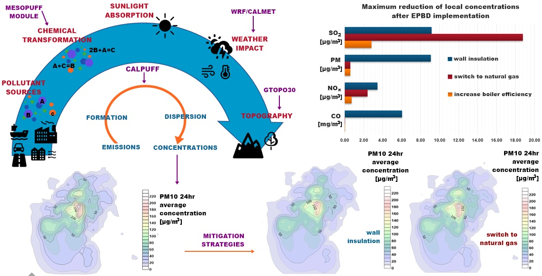
:The high concentration of pollutant sources, complex topography, and regional meteorology are all factors that may contribute to air episodes in dense urban areas. Energy use in buildings is a significant source of pollution in the Greater Athens Area (GAA), Greece, where over 90% of the existing building stock has been classified below energy class B. The present study focuses on the potential effects that a realistic level of building energy efficiency upgrades will have on the air quality over the GAA. Results are expected to be relevant to similar urban areas. Furthermore, the study of primary pollutants’ dispersion is applied at a 1.2 × 1.2 km spatial resolution, providing significant local (neighborhood) level information. Numerical simulations were performed using EPA’s CALPUFF modeling system with wind field input from an independent numerical weather prediction using NCAR’s Weather Research and Forecasting (WRF) model. In order to calculate emission rates from major roads, highways, shipping ports, residential heating installations, and major industrial facilities, data were taken from National and European statistics, demographics, and local topography. After validation, the modeling system was used to examine three building energy efficiency upgrade scenarios, implemented on 20% of the buildings. Ground level concentrations of SO2, NOx, CO, and PM10 were calculated and reductions of up to 9% were found for GAA maximum values but up to 18% for local values that were also close to or above the European safety thresholds.

1. Introduction
Around one-quarter of Europeans are exposed to air pollutant levels exceeding some EU air quality standard [1] in urban areas. Ongoing development projects as well as new legislation related to energy efficiency, such as the Energy Performance of Buildings Directive [2], frequently affect urban air quality although the mechanism is multiparametric and difficult to evaluate [3]. Many efforts have been made to understand the conditions causing air pollution episodes, air pollutants’ accumulation and long-term exposure to them, and domestic heating in particular has been the focus subject of many such studies.
An early study [4] investigated the effectiveness of domestic heating reduction scenarios on urban air quality by applying an EPA dispersion model (ISC-ST) on emission inventories in an urban setting. It was shown that short-term measures restricting the operation of domestic furnaces have little effect on NOx concentration levels, most probably due to the significant effect of meteorological conditions and urban background concentrations. In another study [5], the overall effect of fuel and heating system options on pollutant emissions as well as energy use and the economy were considered. A number of fuels and system alternatives for water and space heating were evaluated. In terms of fuels, natural gas was found to be the preferable choice while for heating systems, even for the same energy source, central and district systems provided up to 20% savings compared to individual ones. Focusing especially on biomass burning for domestic heating, it was found [6,7] to significantly increase PM10 concentration levels. In another study [8], PM2.5 concentration levels were found to be higher during winter periods and were attributed to the use of fossil fuels for domestic heating. Several common heating sources were analyzed and classified based on direct (local) and indirect emission generation. Surprisingly, modern combined heat and power (CHP) systems were found to produce more direct emissions with gas compared to coal, because coal CHP systems have a higher heat to electricity ratio. However, when coal is used outside a CHP system (e.g., scattered use in rural areas) the direct emissions are much higher than any CHP system. In urban settings with high population density, and therefore heat load demand, the emissions per unit land area are high and building insulation measures are proposed as a measure to reduce heat consumption. However, it has also been noted [6] that meteorological variability has a major effect, which could explain more than 90% of the day to day differences in outdoor concentration levels.
Overall, a number of studies (see, e.g., in [6,7,9]) stress the importance of policies and incentives to influence the choice of space heating systems. In a typical example [9], a wide range of urban PM10 and NOx air pollution policies were evaluated in terms of environmental, economic and sociopolitical aspects. Among other measures, the study looked at reduction of indoor temperature setting in residential buildings, banning of residential biomass heating systems, banning of diesel fueled domestic boilers, and energy efficiency refurbishment in residential buildings. Reduction of building inner air temperatures (effectively reducing losses and heating loads) was found to be the most promising measure next only to fostering bicycle use. Recently, data analytics have also been used to examine the relation between heating requirements and reduced air quality standards in cities [10]. Principal component analysis was used [10] to develop an air quality index associated with building space heating energy requirements and the most influential measures were found to be improving boiler exhaust performance, district heat system efficiency and the effects of user behavior (energy use). The effects of vegetation (“greening the city”) seemed to be offset by the fact that plants are inactive in the winter period. In an analysis of households in 22 different Chinese provinces [11], taking into account each city’s regional features, it was again found that district heating is the optimal choice for urban settings, compared to individual systems.
It is clear from the previous survey that building heating system, fuel choice and meteorological parameters have been found by many researchers to be highly influential to urban air pollution. In search of a deterministic relationship between emissions and pollutants’ concentrations, air quality dispersion models that include some form of weather simulation have been widely applied [12] in order to more explicitly take into account meteorological conditions and topography. Such models allow air quality simulation under different scenarios and may lead not only to a better understanding of the observed concentrations but also to an evaluation of future environmental strategies [13].
A combination of EPA’s AERMOD modeling system and a computational fluid dynamics analysis has been used [14] to focus on the use of natural gas fired CHP systems in urban settings and specifically on local air pollution. The dependence on meteorological conditions was verified but also a higher than expected impact of building downwash effects for the dense urban structures. Another model was developed [15], using UWG and Envi-met software, to study the environmental impact through the universal thermal climate index (UTCI) of building energy efficiency. The model was tested on a district of Bologna, Italy, aspiring to connect UTCI and the effects of weather (solar and wind), vegetation, urban, and building materials and user behavior on building energy performance. However, ambient air pollution was not considered in the study. Combining a mesoscale numerical weather prediction model with a dispersion model has been done before (see, e.g., in [16]) but the focus is usually on the modeling effort and the thermal environment instead of linking building energy performance to urban air pollution. These approaches are similar to the one presented here with a major advantage being a spatial resolution that potentially provides detailed information at the local, neighborhood level, rather than area maximum or averaged values, which was the focus of a previous study by the authors [17]. Here, the same methodology is used, in order to include the above-mentioned dependence of urban air pollution on meteorological conditions, and we apply a number of building energy efficiency improvement scenarios to change emission rates with their distribution calculated based on local demographics.
The Greater Athens Area (GAA) belongs to the region of Attica, Greece and is topographically complex, with an irregular coastline, surrounded by high mountains to the east, west and north. It is the most populated area in Greece, hosting 3.8 million people [18] on approximately 450 km2, i.e., a population density of ~17,000 people per km2. The climate is Mediterranean with wet mild winters and hot dry summers. Daily mean temperatures range from 10 °C in the winter to 26 °C in the summer and the dominating winds blow from NE and SW, directions which coincide with the geographical axis of the basin [19]. The combination of topography, meteorology (temperature inversions and sea breeze), and anthropogenic activities such as traffic, residential heating, shipping, and industrial emissions [20] have caused air pollution episodes in the past [21,22]. The ongoing economic recession has affected pollution sources, especially road transport and residential heating, leading to lower concentrations of NOx and SO2 but higher levels of smog [23]. Increased building energy efficiency may contribute on a more systematic and controlled basis to the improvement of air quality but its contribution is difficult to quantify.
There are multiple factors related to building energy use that suggest the possibility of effects on urban air quality and justify further study. For example, most buildings in the GAA [24] use local heat production systems based on combustion (oil, gas, and wood/biomass) for residential heating and the byproducts of the process are emitted within the urban core. Therefore, the amount of energy being used, in itself, directly impacts the amount of flue gases released and the concentration of pollutants in the area. This can be regulated by the energy demand of the building, related to heat loss and insulation and also by the efficiency of the heat production process, i.e., that of the burner. Furthermore, the type of fuel directly affects the constitution of the flue gases, e.g., amount of sulfur (S) in the fuel, emission of particulate matter (PM), etc.
The EPA recommends the use of the CALPUFF modeling system [25] for applications on long range transport of pollutants (distances > 50 km) or over complex terrain, in order to account for the spatial and temporal variability of flow fields. The system is a non-steady state Lagrangian puff model designed to estimate transport, chemical transformation and removal of pollutants, while considering time- and space-varying meteorological conditions [26]. The combination of Numerical Weather Prediction (NWP) models with dispersion models has been a growing trend in order to better simulate the effects of local meteorology on pollutant dispersion [27,28,29]. In the present study, concentrations of primary pollutants are estimated using CALPUFF coupled with the Weather Research and Forecasting (WRF) NWP model. Emissions and concentrations of relevant pollutants from road transport, residential heating, navigation, and industrial facilities have been estimated. The performance of the combined systems is evaluated through comparison with measurements from air quality monitoring stations operated by the Hellenic Ministry of Environment & Energy. After validation of the model, different emission scenarios were studied to provide a realistic implementation of building energy efficiency measures, based on the Energy Performance of Buildings Directive (EPBD). Although there have been studies that address air pollution over the GAA [30,31,32], to the authors’ knowledge, this is the first attempt to combine emission estimation and dispersion simulation with detailed reference to the effects on air quality of building energy efficiency measures. Furthermore, the study goes beyond an emissions rate inventory and combines it with effects of local weather and topography to give detailed information on the distribution of pollutant concentration values within the study area.
2. Materials and Methods
The model set-up used here is the same as the one in our previous study [17] but the main aspects are repeated for completeness and to keep basic input information together with the results.
2.1. Model Description
CALPUFF is a multi-layer, multi-species, non-steady state dispersion model. Its puff formulation enables it to address spatial variability of meteorology, nonuniform land use patterns, dry deposition, wet scavenging, and turbulence based on dispersion coefficients derived from either similarity theory or observations [12]. It is suitable for modeling domains ranging from tens of meters to hundreds of kilometers from a source and for predictions for averaging times from one-hour to one year. It can operate with different source types: point, line, area, and volume using an integrated puff sampling function. In the present application, radially symmetric Gaussian puffs are implemented, as they are considered more suitable for far-field applications [25]. For the computation of meteorological parameters, CALMET is used as a preprocessor. For the computation of the wind fields, an initial guess field is combined with observational or prognostic data to create the final wind field. This data can be sourced either from meteorological stations or from gridded prognostic wind fields generated by a mesoscale model like WRF. In the present study, we used the latter, which is usually better at reproducing regional flows without data gaps and in many cases improves model performance [33].
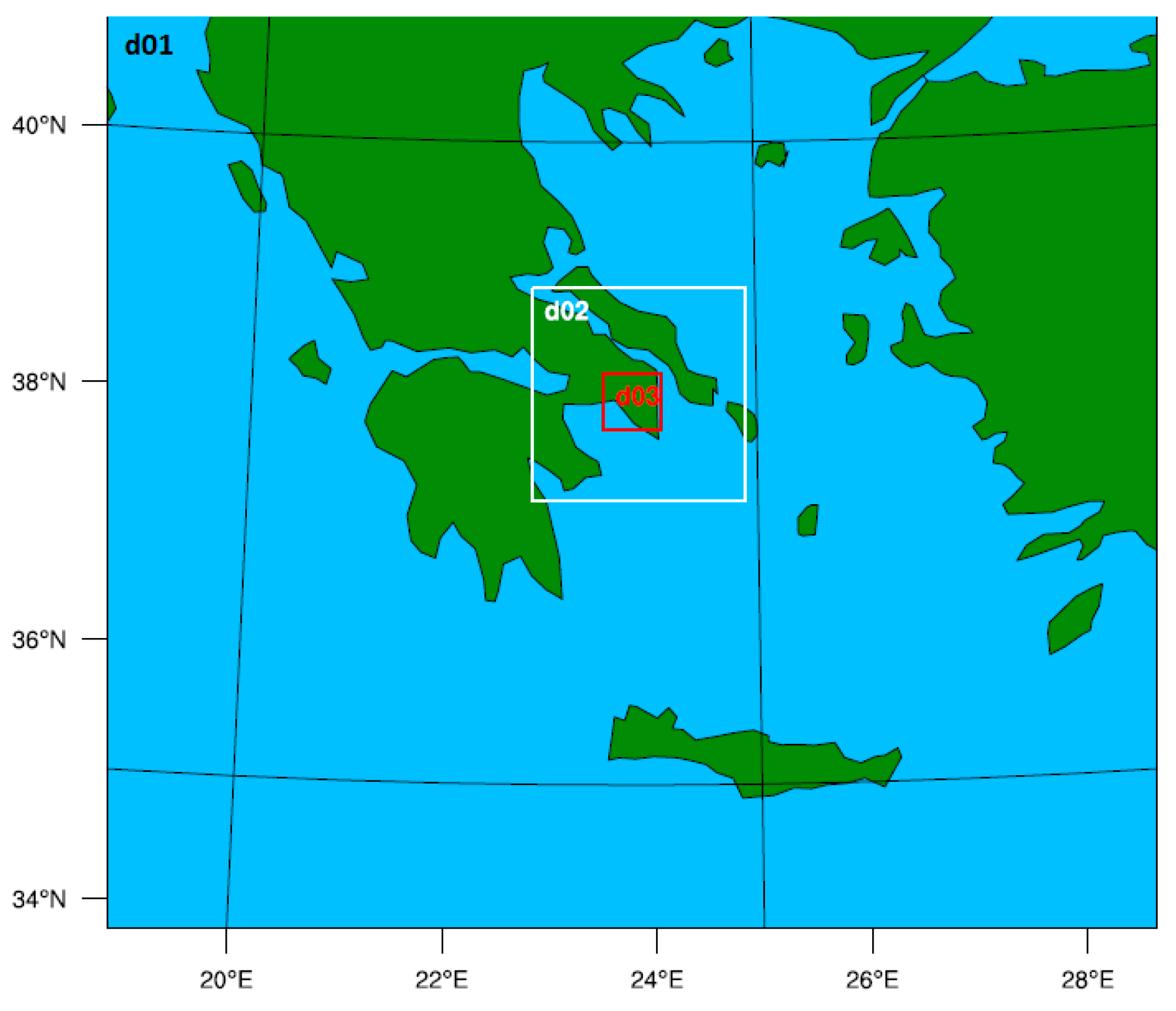
The WRF-ARW v3.7 implementation we used included the following relevant physics schemes: WRF-Single-Moment 3-class (WSM3) microphysics scheme [34], Kain–Fritsch cumulus and convective parameterization [35], YSU planetary boundary layer scheme [36], MM5 similarity surface [37], NOAH [38] with UCM [39] land surface model, and the RRTM [40] and ΜΜ5 SW [41] radiation schemes. Topography was derived from the global 30 s USGS topography data. Initial and boundary conditions were given by the NCEP-GFS (National Centre for Environmental Prediction-Global Forecasting System) global circulation model four times a day. Boundary conditions are updated with GFS forecasts every 12 h for calculation of 48 h WRF forecasts with a maximum time step of 30 s. The WRF model was run on three nested grids (Figure 1) at 45 vertical levels: 12 × 12 km over Greece, 6 × 6 km over Attiki, 1.5 × 1.5 km over greater Athens. The 1.5 × 1.5 km resolution was used as input to CALMET.
2.2. Emissions Estimation and Spatial Allocation
The evaluation period was the week of 10–16 February 2018, for which we estimated emissions of nitrogen oxides (NOx), carbon monoxide (CO), carbon dioxide (CO2), sulfur dioxide (SO2), and particulate matter (PM10) from road transport, residential heating, ship navigation, and industry. As pointed out in an emission inventory [42], air quality in Greece is mostly affected by road transport, navigation, small combustion, and industries. The GAA has the lowest emission contribution across Greece in the agriculture sector while aviation is its lowest emitting sector for PM10 & NOx, which explains why both these sectors were not accounted for in the present calculations of air pollutant emissions in the area.
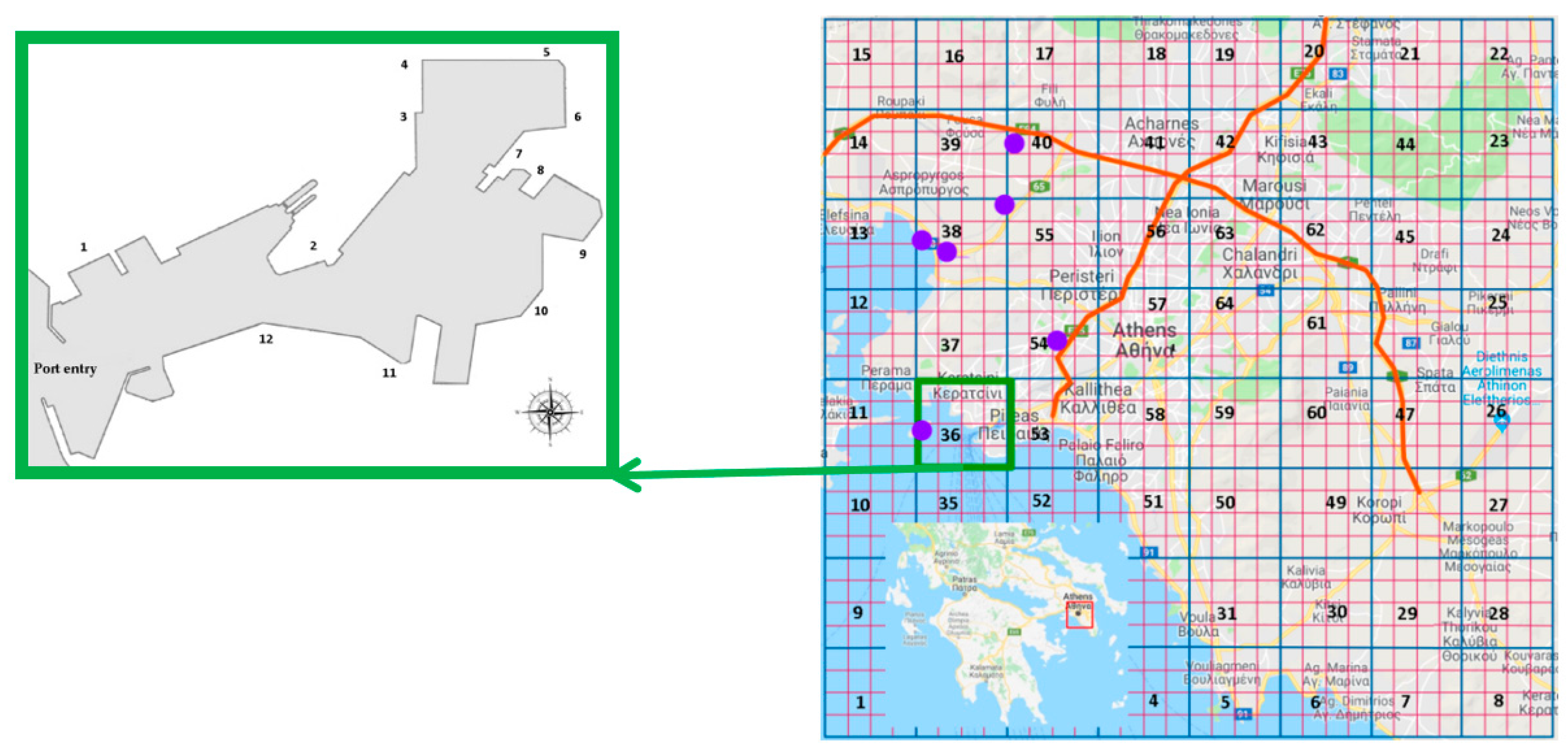
The GAA is characterized by a high population density and the majority of homes heated through distributed systems using heating oil as an energy source [24]. Transport includes underground metro and tram, which do not contribute to local air pollution but also public buses and privately owned automobiles, which do. There are also two large highways passing through the area. Furthermore, there is a large commercial port located to the south and an industrial area to the southwest. These main sources are depicted in Figure 2. Emissions from industrial stacks and national highways were estimated explicitly as point and line sources, respectively. The line sources were simulated using a sequence of coordinates, enough to provide for a sufficient resolution of the road path. All other emissions were modeled as area sources within 64 subdomains, each covering an area of 23.04 km2 and containing 16 predefined square grid cells (dx = dy = 1.2 km), which determined the spatial resolution of the simulation. The study area can be seen in Figure 2: the 1.2 km × 1.2 km grid is shown in red, the 64 subdomain areas in blue, the area of Piraeus port in green, industrial facilities in purple and highways in orange.
2.2.1. Road Transport
Road transport is accountable for approximately 20% of total CO2 emitted in Europe and although these emissions are dropping (e.g., by 3.3% in 2012), they are still 20.5% higher than 1990 [43]. Due to differences in engine operation, it is common practice to differentiate between urban and rural roads or highways [13] when examining vehicle emissions. Directly applicable data for road traffic emissions in Attica during the simulation period were not available but the European Monitoring and Evaluation Program (EMEP) has provided sector data for Greece for the year 2016 [44]. According to a road transport inventory for Greece and Attica for 2006–2010 [20], 40% of national CO2 and CO and 30% of NOx and particles are emitted in Attica. Emissions from urban roads were estimated and spatially allocated on each of the grid cells in Figure 1 using the following scheme,
where is the emission (in mass) of pollutant i in grid cell x, is the annual total mass emission of pollutant i, is the population in cell x, is the total population for the entire domain, with population data obtained from ELSTAT [18]. Emissions from the two national highways seen in Figure 2 were estimated based on the hourly traffic count (HTL), measured in number of vehicles on road segment length L (km) [45] using as the emission factor [46] for pollutant i, vehicle type k and engine technology j (tonnes/km/vehicles). For the present study, we included passenger cars, light commercial vehicles, heavy duty vehicles, buses, and motorcycles. Rural emissions were not considered since GAA is an urban area [47]. Annual emissions from road transport for Greece and Attica, are shown in Table 1.
2.2.2. Small Combustion
Following the EMEP/EEA [46] classification, small combustion comprises five different groups: open fireplaces using wood, small size (<50 KWth) boilers using oil, medium size (50 KWth–1 MWth) boilers using oil, boilers using natural gas, and finally stoves using natural gas. The declining income in Greece during recent years has led to the extensive use of, otherwise decorative open fireplaces found in urban dwellings, as means for domestic heating [48]. The GAA in particular has experienced smog formation during winter months because of residential wood burning, an increasingly frequent occurrence during the years of the financial crisis [49]. The emissions of relevant pollutants (SO2, NOx, CO, and PM10) were determined using a technology specific approach [46] based on
where is the default emission factor of pollutant i for source j and fuel k (g/GJ), and is the annual consumption of fuel k in source type j (GJ). The annual consumption of thermal energy in a typical Greek household was considered [50] as was the share of fuels used for residential heating in Attica [51]. Spatial allocation of emissions was made possible using population and housing data [18] so that each area of the grid corresponded to a number of households. Boiler and fuel type emission factors are given in Table 2.
2.2.3. Navigation
Although ship emissions in port account for a small percentage of the total emissions from ship activity [52], they are the most relevant to urban air quality for port cities [53]. There are a limited number of studies focusing on port emissions and only a few for the port of Piraeus [30,54]. We estimated emissions from passenger and container ship navigation in the port of Piraeus for the exhaust pollutants SO2, NOx, PM10, and GHG (CO2). Standard approaches depend on the available data so emissions can be estimated through a default approach (Tier I), a technology-specific approach (Tier II) or a ship movement methodology (Tier III) [46], which was the one applied here according to
where is the emission of pollutant (i) over a complete trip (tons), LF is the engine load factor (%), P is the engine power (kW), T is time (h), EF is the emission factor (kg/ton) depending on type of vessel: e is the engine category (main or auxiliary), j is the engine type (slow-, medium-, and high-speed diesel, gas turbine, or steam turbine), m is the fuel type (bunker fuel oil, marine diesel oil/marine gas oil, gasoline) and finally p is the different phase of trip (maneuvering or at berth). The Hellenic Ministry of Shipping and Island Policy announces daily departures of passenger ships from the port of Piraeus [55] and their engine information was taken from the work in [56]. The engine load factors and the emissions are shown in Table 3 [46,57]. All ships in port were driven by medium speed diesel (MSDs) and used Low Sulphur Fuel Oil (LSFO) fuel (containing maximum 1.5% sulfur content by mass, as required by EU Directive 2016/802/EU [58]) for their main engines. From the 21 ships found at port, 14 used a diesel-electric engine configuration and seven were driven by diesel engines while their auxiliary engines burnt medium speed diesel oil (MSD; 1% S). To calculate maneuvering time, information on the destinations of the vessel was used to locate its position at berth, as Piraeus port has dedicated berthing positions per destination. The entry to berth distance varied between 0.3 and 1.9 km and the inbound speed was an average of 9.26 km/h and the outbound 14.82 km/h. Another 6 min were added for docking and 3 min for undocking while an average time of 8h at berth was assumed for each ship [30].
The area and layout of Piraeus port is shown in Figure 2. The Tier III [46] approach was also applied for the estimation of emissions from the container terminal of Piraeus, using data from Marine Traffic [59], which provides the number and type of ships located in ports. Main engine power, average cruise speed, average duration for in-port activities and emission factors were obtained from EEA’s guidebook [46] (Table 4) depending on the type of ship and the fuel used.
The dominant fuel/engine type was chosen for each ship category based on the percentages of installed main engine power by engine type/fuel class found in the guidebook. The ship categories present at the port during the week of simulation were liquid bulk carriers (LBC), dry bulk carriers (DBC), containers (C), general cargo (GC), Ro-Ro cargo, tugs (T), and others (O). For all of them, main and auxiliary engine load factor while maneuvering was 0.5. At berth, it was 0.2 for the main engines, 0.6 for LBC’s auxiliary engines and 0.4 for all others’ auxiliary engines. Engines vary from slow speed diesel (SSD) to medium speed diesel (MSD) and to high speed diesel (HSD) while fuel types are either bunker fuel oil (BFO) or marine diesel oil–marine gas oil (MDO–MGO).
2.2.4. Industry
The European Pollutant Transform and Release Data Registry (E-PRTR) [60] contains industrial activity data for the year 2016. A facility is required to report data under E-PRTR if it releases pollutants that exceed thresholds specified for each medium—air, water, and land. The registry contains annual data reported by more than 30,000 industrial facilities covering 65 economic activities within nine industrial sectors: energy, production and processing of metals, mineral industry, chemical industry, waste and waste water management, paper and wood production and processing, intensive livestock production and aquaculture, animal and vegetable products from the food and beverage sector, and other activities. For the area modeled, six facilities met the criteria and emissions were allocated to grid cells using the coordinates of each facility (purple dots in Figure 2). Data required by the model concerning stack height and stack diameter, exit velocity, and exit temperature of pollutants were gathered from relevant sources [61,62].
2.3. Numerical Implementation
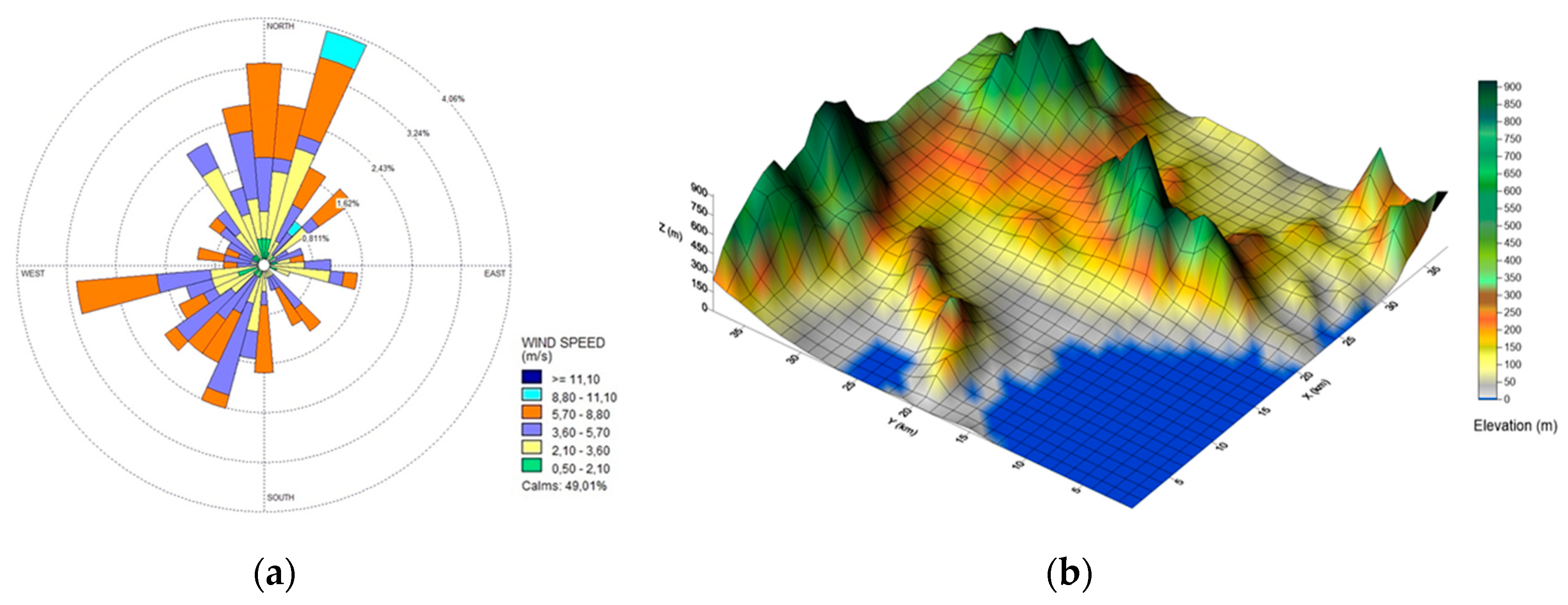
The steady-state CALPUFF modeling system was used for the calculation of concentration fields, implementing WRF results to the CALMET meteorological preprocessor for detailed wind field data. The GAA basin is surrounded by high mountains from the NE, NW, and SE and the sea from the SW with winds blowing mainly from N-NE and SW. The chosen simulation period was representative of typical winter conditions for domestic heating. Average temperatures and average absolute maximum and minimum temperatures for February in Athens are (10.6, 22, 1.5) °C, respectively with an average wind speed of 2.1 m/s [63]. For the examined period, the same temperatures were (9.98, 17.3, 4.1) °C and the average wind speed was 5 m/s, i.e., typical temperatures and slightly stronger winds than average, blowing towards the sea. The prevailing winds during the week of simulation (10–16 February 2018) and gridded terrain elevation of the modeled area can be seen in Figure 3 [64].
Emission source input for the modeling system was split into three different categories: six point sources representing industrial facilities, 91 line sources representing the two national roads, and 64 area sources. Each area source was 4.8 × 4.8 km2 in size, corresponding to the 64 subdomains of Figure 2. One area source corresponded to the port of Piraeus while the rest represented sources of road transport and residential heating. All sources were overlaid onto the computational domain, which consisted of a uniform grid with square cells of 1.2 × 1.2 km2 in size. Point and line sources were allocated directly to the computational grid but the larger area sources were uniformly distributed onto the denser grid cells. Table 5 summarizes the estimated emissions in the modeled domain for all types of sources. Emissions of CO2 were not modeled for the source category of residential heating due to lack of emission factors data [46]. It should be noted that emissions from industrial sources are considered underestimated since only industrial facilities which exceeded E-PRTR threshold were included.
It can be seen from Table 5 that residential heating is a major source of emissions for CO, SO2, and PM10. However, it should be kept in mind that this source is distributed throughout the computational domain, as opposed, e.g., to industry and navigation which are much more concentrated in specific areas and will significantly influence local concentration levels despite lower emission factor values. In mass terms, the pollutant emitted the most in the GAA is carbon monoxide, formed mainly from incomplete combustion of fuels, followed by nitrogen oxides. Road transport contributes to the majority of CO emissions and to about half of the NOx that is emitted in the air. This is also in agreement with EPA findings [65]. For PM emissions, residential heating dominates as an overall source, which can be justified by the increasing use of wood as a combustion source during winter in Athens [49] (Table 2).
Temporal resolution of the simulation was 1 h, corresponding to the available meteorological data. Pollutant concentrations were estimated for all hours from the 10th to 16th February 2018 at 1024 gridded receptor positions. Chemical transformations were parameterized using the five species scheme (SO2, SO4=, NOx, HNO3, and NO3-), as included in the MESOPUFF II default reaction algorithm [26]. Pollutants’ estimated average concentrations were compared with the health-based standards included in the European Directive 2001/81/EC [66] (Table 6).
2.4. Definition of Scenarios to Evaluate Impact of Building Energy Efficiency on Air Quality
In order to estimate the effects of building energy efficiency interventions on air quality in the GAA, three different scenarios of implementation of the European Directive on Energy Performance of Buildings [2] were investigated.
The Energy Performance of Buildings Directive [2] along with the Energy Efficiency Directive [67] promote the improvement of energy performance of buildings within the EU. One of the goals of the EPBD and its revision [2] is to promote the cost-effective renovation of existing buildings [68]. We focused on the existing building stock and priority was given to energy performance improvement interventions related to the building envelope (thermal insulation of walls, windows, doors, ceiling, etc.) and the equipment (more efficient heating, cooling systems, ventilation, etc.). The Greek Regulation on the Energy Performance of Buildings (KENAK) has set energy class B as a minimum requirement in energy performance for new buildings and buildings undergoing major renovations. According to Greek law, a renovation is considered major when the total cost is higher than 25% of the value of the building, excluding the land value upon which the building is situated [69]. For the GAA, it was found [70] that 78.66% of the existing building stock is classified below energy class B. Based on a report published by the Greek ministry for the environment [71], which studied different measures on the existing building stock and calculated thermal and electrical energy savings for each, we formulated three different renovation scenarios with their respective savings effects:
- insulation of walls resulting in thermal savings ranging from 33% to 60%,
- increase of boiler efficiency resulting in thermal savings up to 17%, and
- replacement of fuel oil boilers with natural gas boilers resulting in thermal savings up to 21%.
Renovation scenarios were limited to buildings that do not belong to an acceptable energy efficiency class, namely those from energy class H to C. We assumed an implementation rate of 20% as an optimistic projection of the future, even though available information estimates a value that does not exceed 3% [72].
3. Results
3.1. Validation
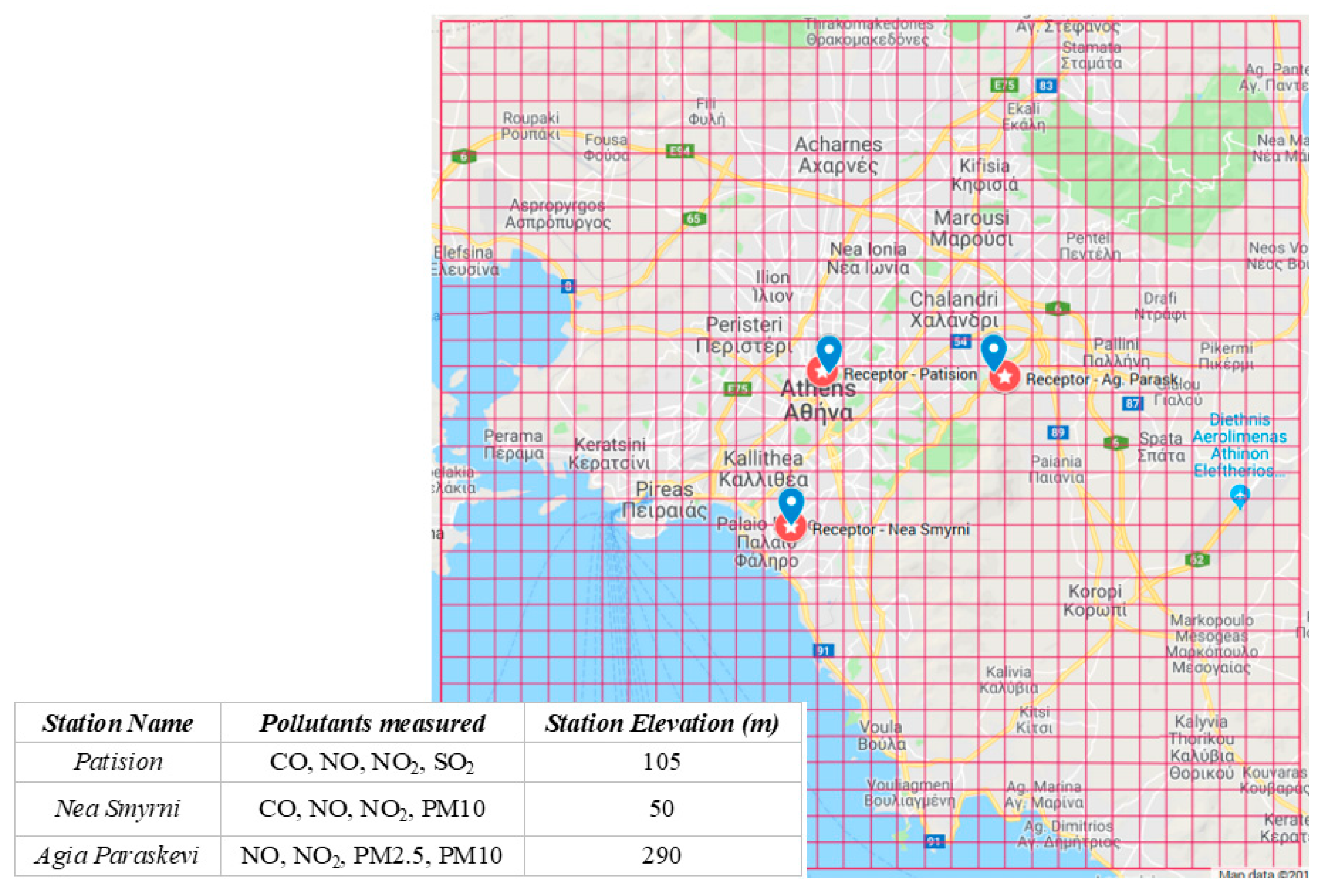
For validation purposes, we compared the estimated concentrations with available measurements at three monitoring stations operated by the Ministry of Environment & Energy [73]. We chose Patision St. in the center of Athens, monitoring CO, NO, NO2, and SO2, Nea Smyrni further south, monitoring CO, NO, NO2, and PM10 and Agia Paraskevi to the north, monitoring NO, NO2, PM25 and PM10 (Figure 4).
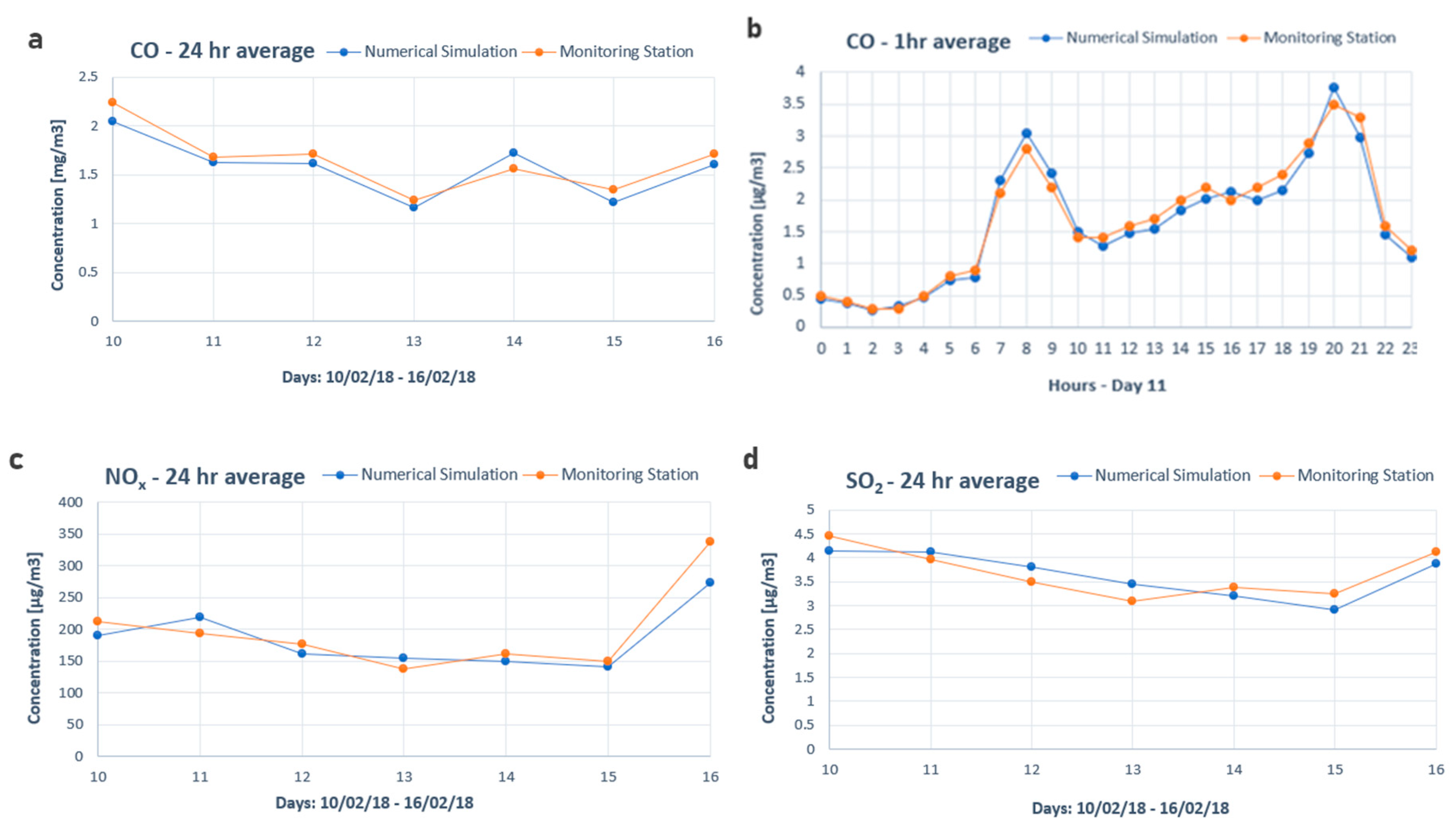
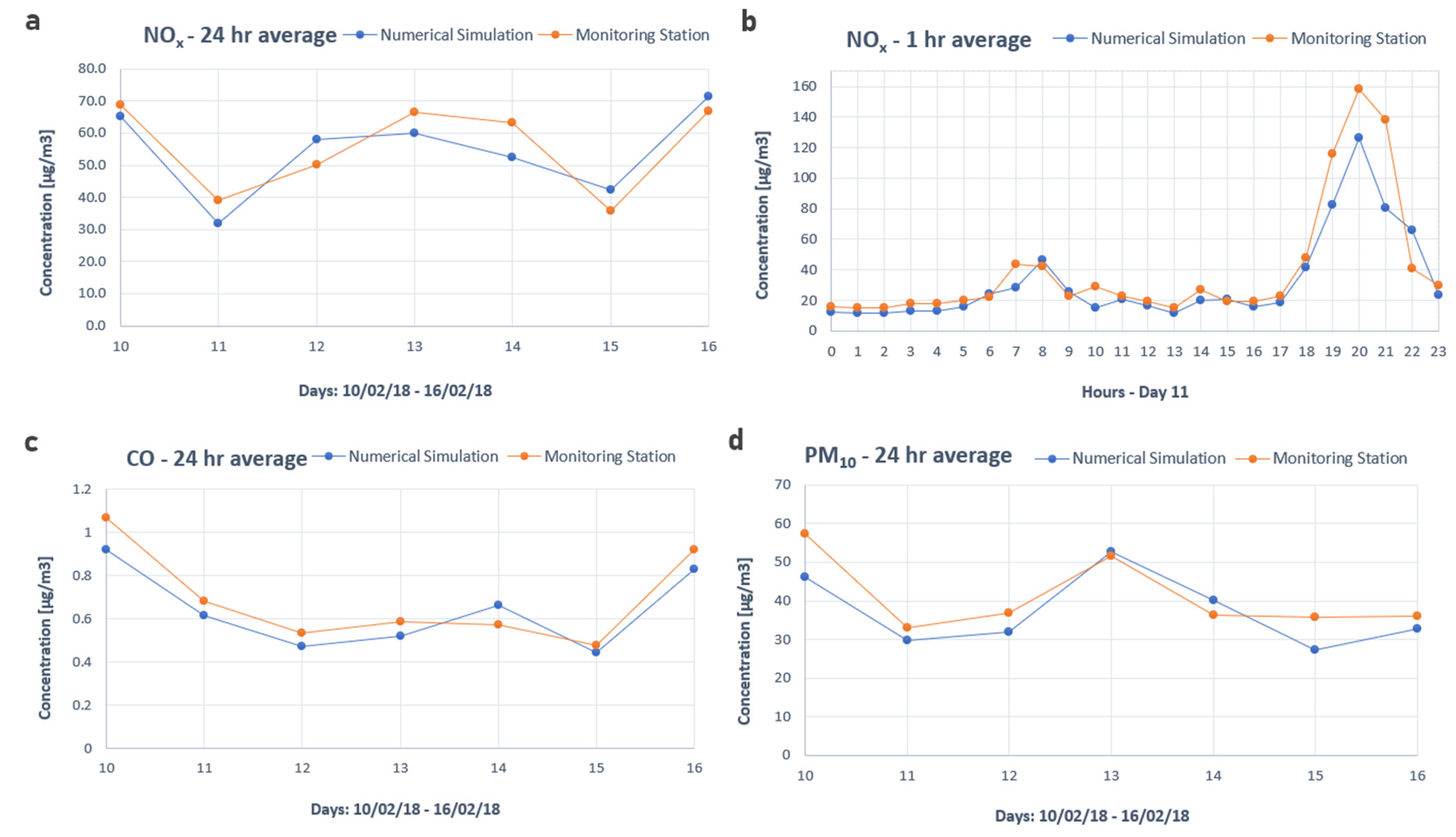
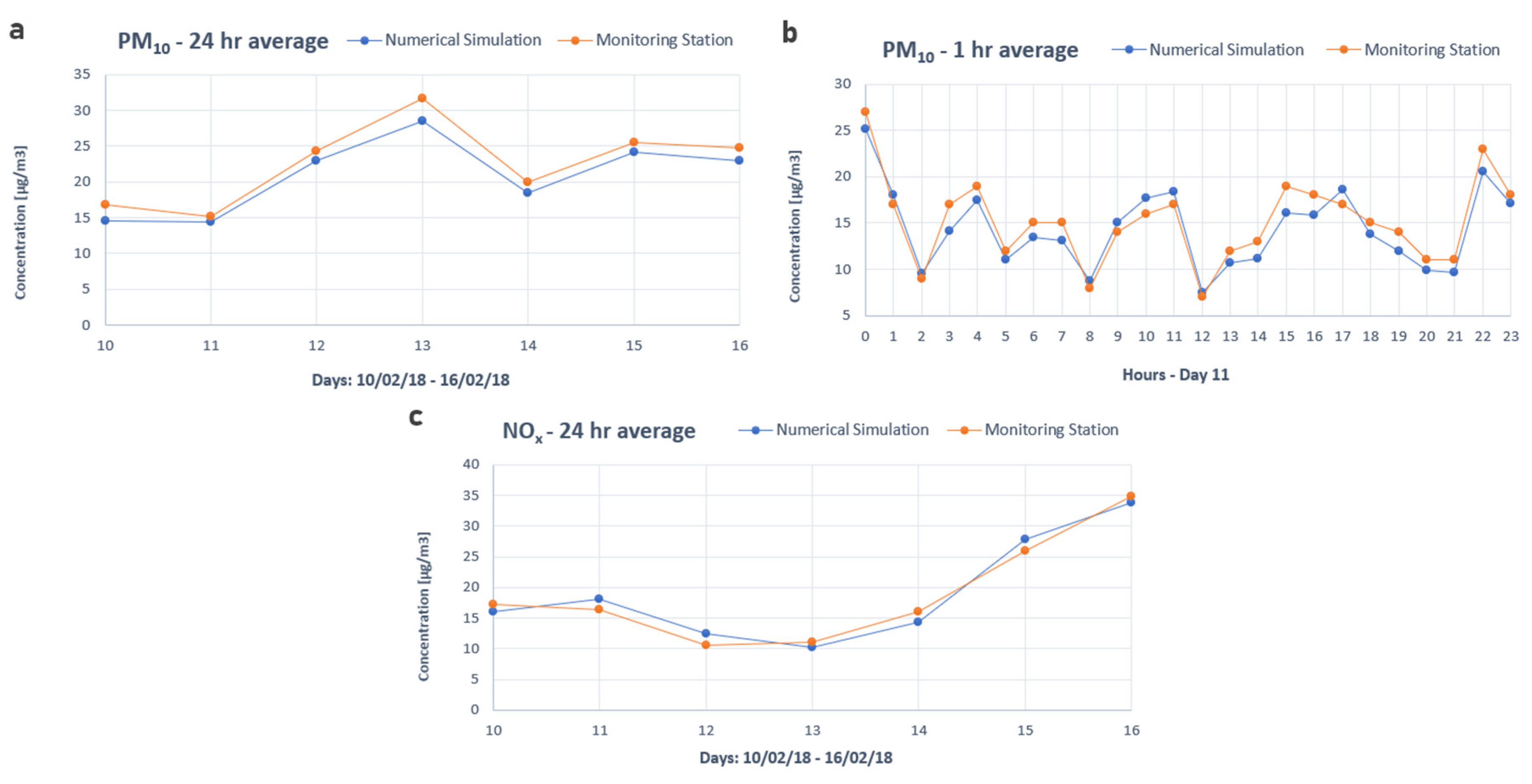
Comparison of the results of the present simulation with measured values [73] included daily time series of concentrations for the entire week of simulation and, for selected pollutants, hourly time series during a specific day. Predictions of weekly and hourly time series are presented in Figure 5, Figure 6 and Figure 7.
The results (Figure 5, Figure 6 and Figure 7) showed good agreement with Nea Smyrni NOx predictions (Figure 6b), exhibiting the largest deviations from the monitoring station measurements. A possible explanation is related to the sources due to road transport. Syggrou avenue, which passes through Nea Smyrni, is one of the busiest roads in Attica and the estimation of its emissions was based on local population data and not hourly traffic flow, which could justify the difference. Another point of discrepancy is the concentration of NOx, possibly because it depends on chemical transformations that define the NO2/NOx ratio, and are subject to a number of uncertainties. Although not visible in the present validation results, we also expect some discrepancies near the industrial zones, to the south west of the computational domain, as there is an information gap with regard to industrial pollutant emissions in the GAA, also evident in other reports e.g., in the Industrial Inventory of AIRUSE Cities, which did not include Greece due to lack of data [74].
3.2. Distribution of Major Pollutants
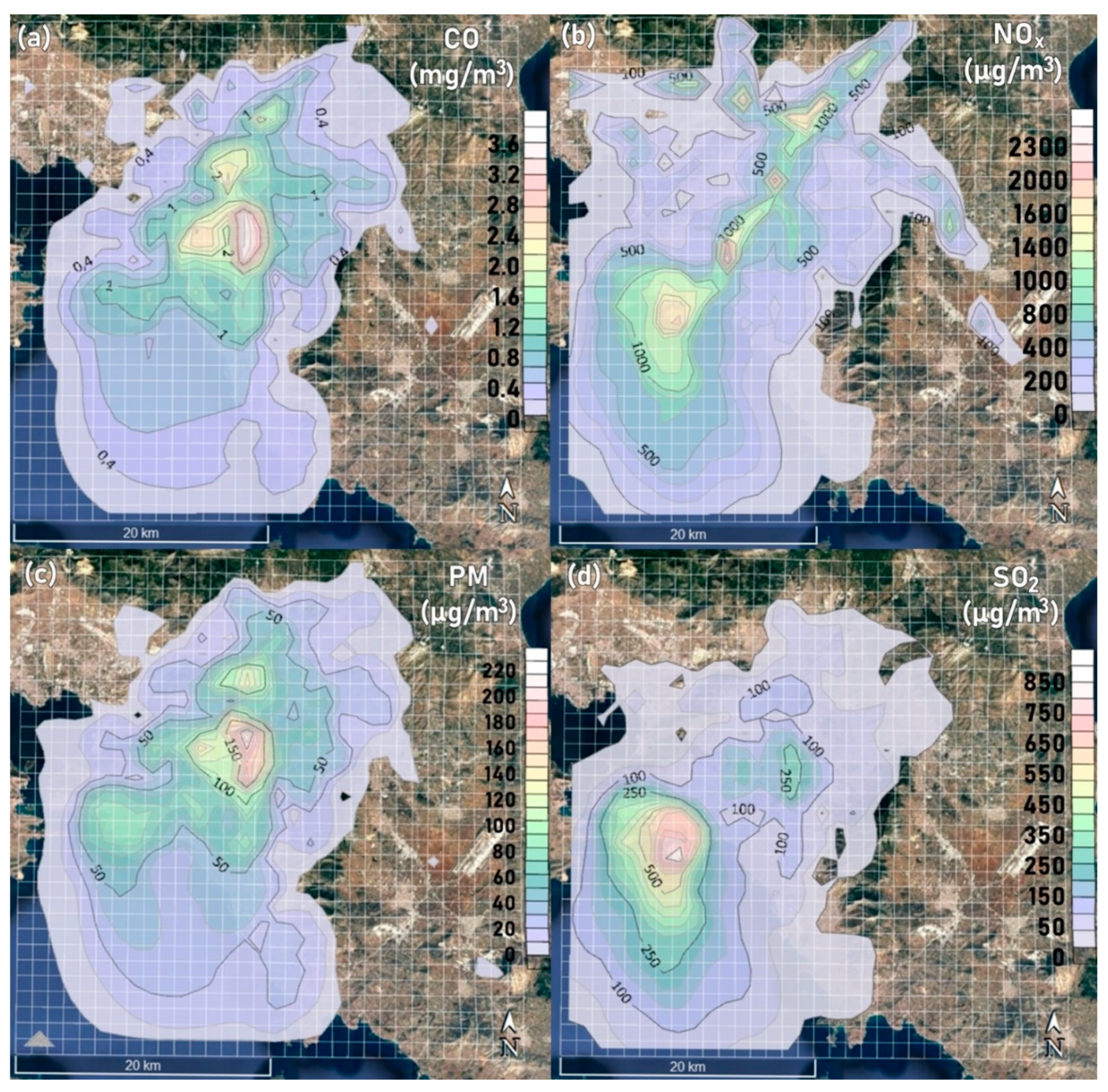
Ground level spatial distributions of averaged pollutant concentrations for the entire period of simulation are shown in Figure 8. Spatial distribution is presented in the form of colored contour regions, overlaid on a map of the area.
Maximum concentrations of CO and PM10 (Figure 8a,c) are observed in central Athens, which covers 35 out of the total 66 municipalities. The most polluted gridded areas in this source category include Peristeri and Aigaleo (No 54), Patisia (No 56), the municipality of the City of Athens (No 57) and finally Kalithea and Nea Smyrni (No 58), (numbering corresponds to subdomains of Figure 2). These areas’ dwelling stock is among the highest in the GAA [18]. High values of NOx concentrations (Figure 8b) can also be discerned in central Athens and along the major highway in the SW-NE direction (Figure 2) while Piraeus Port (Figure 2) shows the highest concentration of SO2 (Figure 8d), due to the sulfur content of marine diesel fuel.
Proceeding beyond the current status, simulations were performed for the three building energy efficiency improvement scenarios, using different emission rates for domestic heating sources each time, according to the expected thermal savings (see Section 2.4). The rate of implementation for each scenario, assumed at 20%, was uniformly distributed throughout the simulation area. Table 7 shows the area averaged emission rates before and after implementation of the three scenarios:
a. Insulation of walls. Renovation of the residential building stock with available heating by applying thermal insulation to the building envelope, regardless of the fuel or boiler type used in their heating system. This measure is expected to result in a reduction of ~45% in buildings’ thermal energy requirements [71], and therefore in fuel consumption for heating, regardless of the fuel type. The resulting changes in pollutant emissions correspond to a maximum reduction in the area averaged total emission rate from all sources of over 8% for PM10 (Table 7).
b. Boiler Efficiency improvement. The second scenario assumes an increase in boiler efficiency. The potential for savings in thermal energy demand is 15% [71], which affects only the proportion of houses using heating oil as a fuel source. Maximum reduction in the area averaged total emission rate from all sources is just over 1% for NOx (Table 7).
c. Replacement of fuel oil with natural gas. In the third scenario, a switch from oil to natural gas was assumed and thus a 20% reduction in buildings’ thermal energy consumption from oil [71]. Expected maximum reduction in the area averaged total emission rate from all sources is almost 4% for NOx (Table 7).
As the emission rate (Table 7) is an area average, it is then multiplied by the population density (as a fraction of the total population in the GAA) in order to define local emission rates for each grid cell area (Figure 2). It should be noted that the decrease in the emission rates presented in Table 7 is the basis for the subsequent calculation of the pollutant concentrations and does not necessarily reflect the change in these concentrations. Variations in population density interact with topography and weather conditions in the dispersion modeling phase (CALPUFF) to give the resulting ground level concentrations. The most notable reductions in ground level maximum concentrations were 8.76% for the PM10 24 h average and 5.11% for the CO 8 h average concentration for the wall insulation scenario (a) and 1.2% for the SO2 1 h average concentration for the replacement of fuel oil to natural gas (c) scenario. These values are higher than the decrease presented in Table 7 and this should be attributed to the combined effects of population density distribution (which affects emission source distribution), topography and meteorology. The effects on ground level concentrations when implementing boiler efficiency scenario (b) were insignificant (<0.5%). In the case of PM and SO2, the maximum concentration values were well above the limits recommended by the EU directive [66] and this indicates that there are also other locations within the GAA where these limits are exceeded.
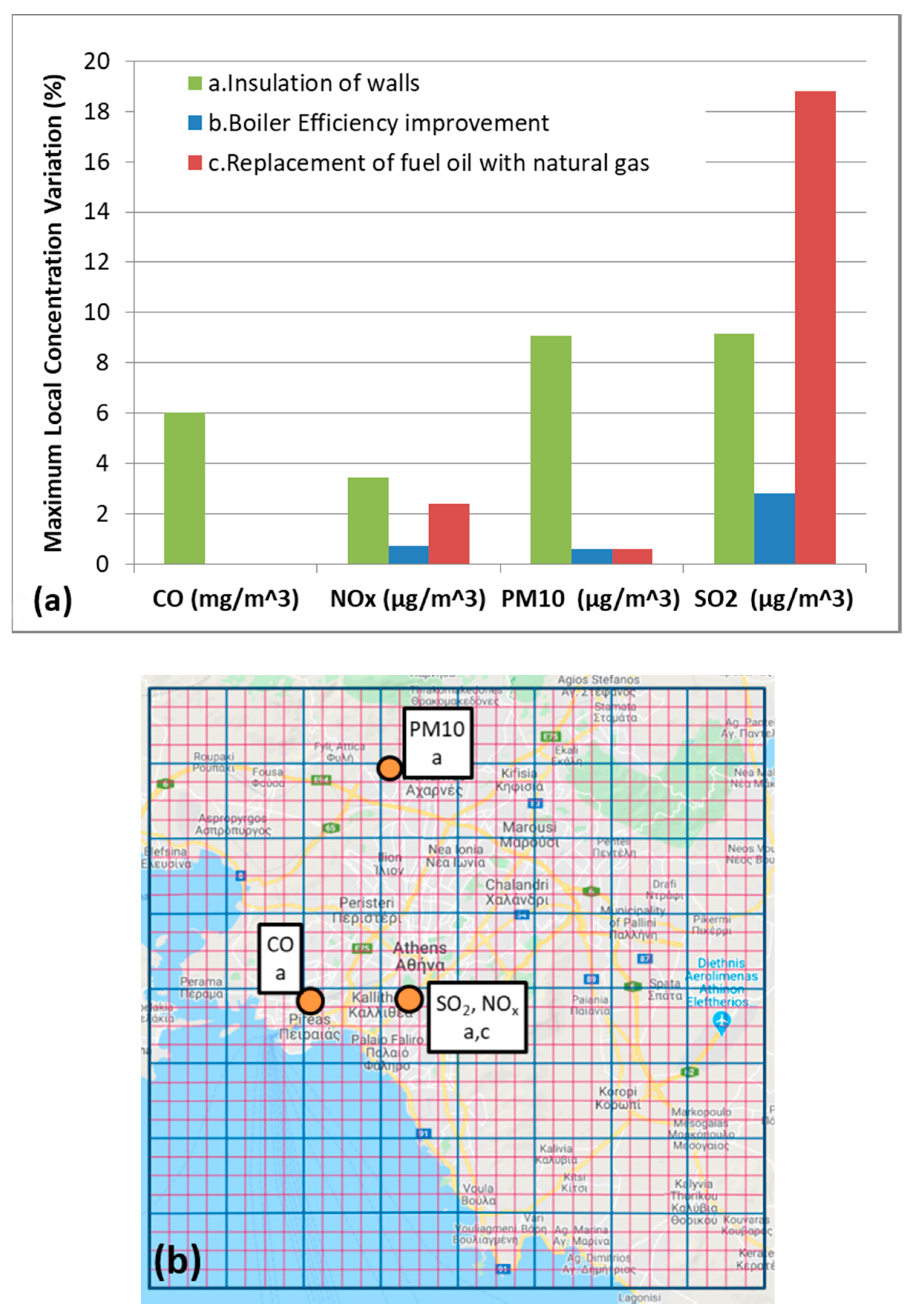
As previously stated, highways, and especially Piraeus Port, are strong localized sources of NOx and PM10 and the port is the major contributor to SO2 in its vicinity. On the other hand, residential heating is distributed throughout the GAA and, in addition to overall area maximum values, energy efficiency measures will also influence local concentration levels that may also be significant. However, examining local value variations can be misleading without taking into account the absolute concentration values since large percentile variations may appear for very low local concentrations. To overcome this, we focused only on local concentration values that were larger than an arbitrarily chosen value of one tenth of the maximum, i.e., Cmax/10. Results are presented in Figure 9.
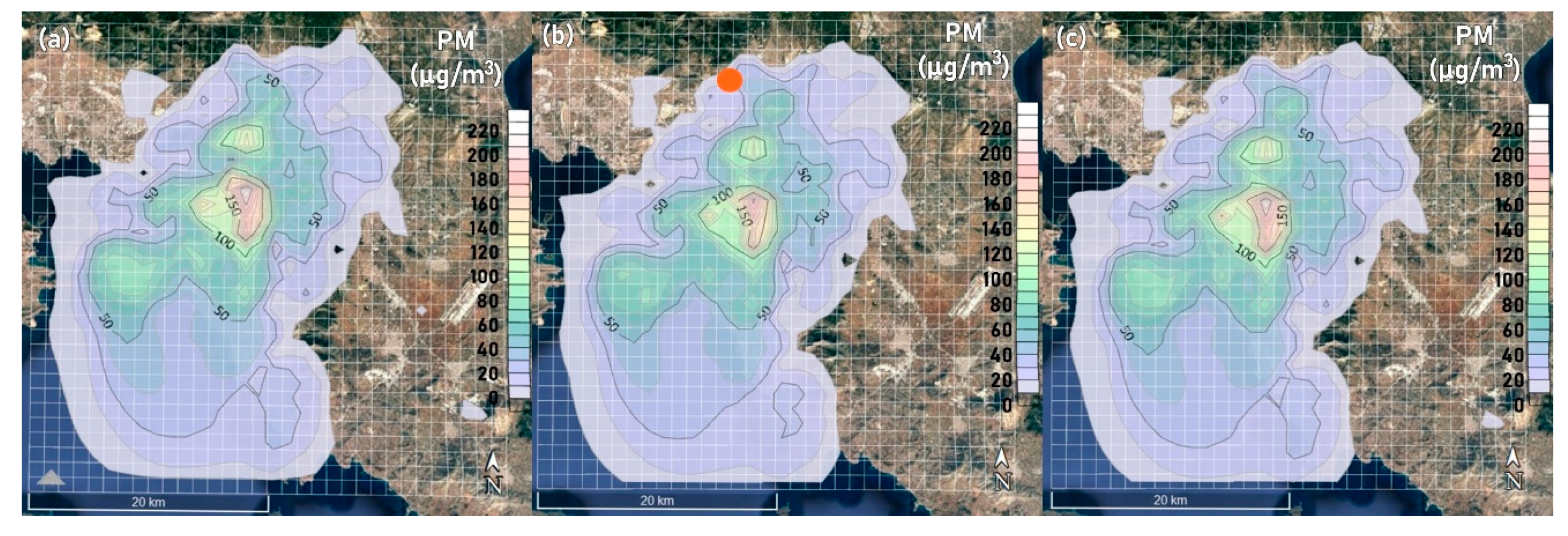
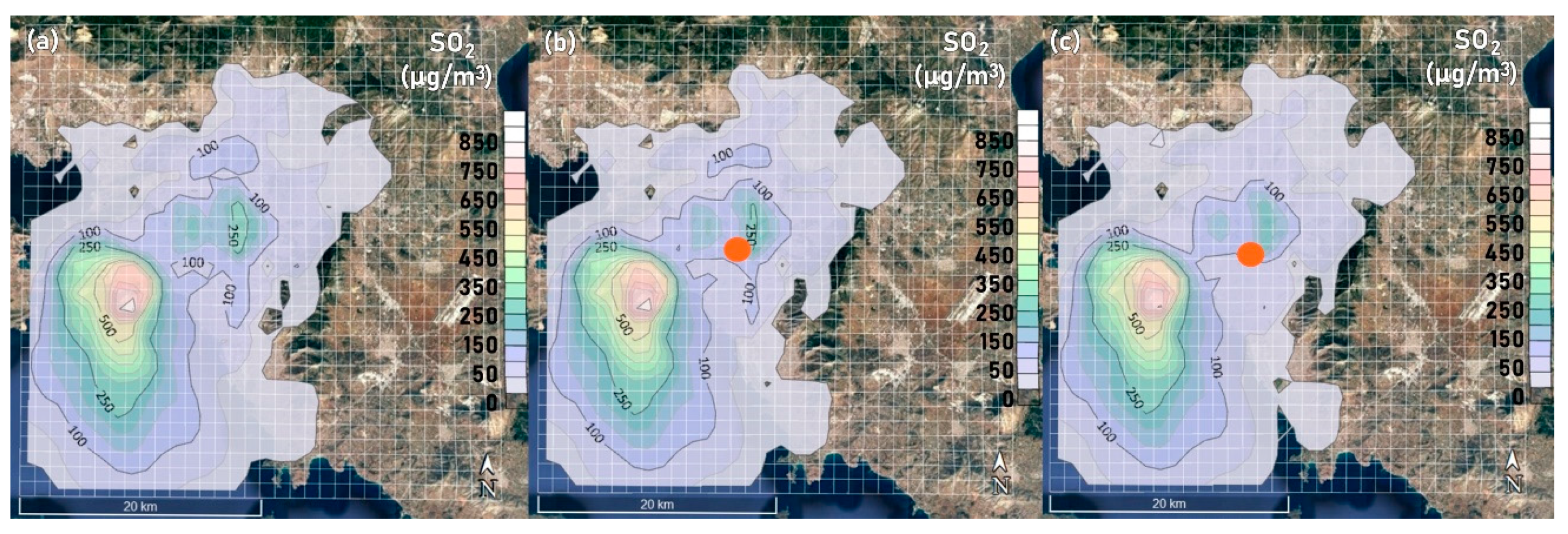
The effects on CO are generally small to insignificant and, in any case, the maximum values are well below the limit. Although overall maximum NOx concentrations in the GAA are not affected by the energy efficiency scenarios, this is because localized sources such as Piraeus port and highways are the main emitters. However, at a local level, there are areas with NOx concentration levels well above the limit where a 2–3% reduction is observed (Figure 9). For PM10, there are still significant reductions of ~9% with the wall insulation scenario (a) for local 24 h average values down to ~30 μg/m3, which is still close to the 50 μg/m3 limit and therefore non-negligible for air quality considerations. This occurs in the northern part of the area, as indicated in Figure 9b. The case of the SO2 1 h concentration values is also notable. Although reductions in the range of only ~1% were observed for area maximum values, this is due to the limited domestic heating contribution in the port area, where ship emissions dominate and the GAA maximum appears. However, there are densely populated neighborhoods (see Figure 9b) where domestic heating is the main source of SO2 and wall insulation leads to a 9% reduction and conversion to natural gas leads to a 19% reduction in ambient SO2 concentration levels. These are areas with local 1 h average SO2 concentration values of ~230 μg/m3, very close to the limit of 350 μg/m3 [66] and therefore highly relevant to air quality. Although NOx reductions are smaller, it is notable that the location of maximum reduction coincides with that for SO2 (Figure 9b). Benefits from the improvement in boiler efficiency (Scenario b) are limited. Contour maps of the overall effects on concentration distributions for PM10 and SO2 are presented in Figure 10; Figure 11.
Figure 10 shows the higher concentration of PM10 in the densely populated urban area, where the largest contribution is from wood burning for residential heating. The wall insulation scenario (Figure 10b) directly reduces heat losses and therefore heating requirements, affecting all heating sources, including wood burning. Scenarios (b) and (c) improve efficiency but only for oil type heating sources, leaving wood burning intact and thus leading to minimal effects on PM10 (Figure 10c). For SO2, Figure 11 shows that higher values appear near the port, where ship navigation contributes due to fuel sulfur content. However, there are high concentration levels within the urban area of central Athens as well and building energy efficiency measures directly affect these. The wall insulation scenario (Figure 11b) reduces energy demand, but this happens equally for all fuel sources. When heating oil is substituted with natural gas, SO2 emission per unit energy demand is reduced by two orders of magnitude (Table 2) and the effect on SO2 concentration levels in the urban area of central Athens is pronounced (Figure 11c).
4. Discussion
The building sector is universally regarded as a major contributor to total energy consumption. As such, it has been the target of several energy policies and legislative interventions. Although reducing energy consumption is in itself a worthwhile target, it is directly and closely linked to environmental issues such as atmospheric pollution. In dense urban areas, atmospheric pollution and air quality are significant parameters connected to good health and well-being and sustainable cities and communities, among the other UN sustainable development goals [75]. The Greater Athens Area (GAA) in Greece is a characteristic example of a dense European city with diverse sources of air pollution. As a case study, it could provide insight into the general effects of energy efficiency measures on air quality.
This study estimated spatial and temporal variations of emissions and concentrations of select air pollutants in the GAA during a typical heating week, in February 2018. Pollutant sources included domestic heating, urban transport and highways, port navigation, and major industrial facilities. Validation with measurements at several points throughout the GAA was acceptable and the developed model was then used to assess the effects of selected building energy efficiency measures on pollutant ground level concentration level. Three scenarios of energy efficiency measures were taken into consideration, based on the European Energy Performance of Buildings Directive, which has been in effect for over a decade throughout Europe and has been recently amended [2]. However, since new construction of buildings is very limited, great effort is still required to upgrade the existing building stock with new technology and, furthermore, effects on air quality have not been extensively discussed. To this end, three EPBD based scenarios were examined: application of insulation to building walls, increased boiler efficiency and replacement of fuel oil with natural gas. In all cases, an implementation rate of 20% was assumed uniformly across the GAA.
From the results, it seems that the maximum values in the area are moderately affected by the scenarios that were examined with reductions in area maximum pollutant concentrations reaching ~8%. However, when looking at local values across the simulation area, there are several neighborhoods where local reductions are significantly higher than the reduction in the GAA maximum. It is notable that several of these areas are characterized by high levels of pollutant concentration, even though they may not be the GAA maximum. Building energy efficiency measures affect pollutant sources (buildings) that are distributed throughout the urban area, as opposed to an industry or a port, which are more singular, point sources. Therefore, interventions to buildings affect sources whose locations are more likely to coincide with regions of adverse topography, weather conditions or urban density.
It was found that the most efficient measure to reduce PM10 concentrations locally (by over 9%) was the wall insulation scenario as it directly reduces heat losses and wood burning, which has recently become a major source of urban particulate matter in the winter [76]. On the other hand, although sulfur emissions from marine fuel burning dominate as the maximum source of SO2 in whole GAA, they are found in the vicinity of the port and are relatively insensitive to emissions from domestic heating. However, there are areas far from the port that also exhibit high levels of SO2 concentrations, close to European limits for human health [66], due to burning of domestic heating oil. These were found to be highly responsive to switching to natural gas with local reductions of ~19%. This reduction is very close to the implementation rate of 20% for this measure, indicating that in these neighborhoods, domestic heating oil may be the main source of SO2 emissions.
5. Conclusions
As discussed in many previous studies (see, e.g., in [6,7,8,9]), air pollution is highly dependent on local topography and weather but it is reasonable to expect that the reliability of any scenario simulation will depend on the accuracy and details of the respective inputs (see also [14,15,16]). In the present study, the complex topography (mountainous and coastal surroundings) was directly taken into account through digital elevation maps and detailed hourly weather input, provided by a numerical weather simulation model. This permitted the simulation to be performed at a horizontal spatial resolution of the order of ~1 km2 and validation against measurements proved to be successful.
When analyzing urban air pollution at a high spatial resolution, it is important to take into account local parameters such as local topography, microclimate and building geometry, vegetation, etc. Although the present model attempted to include topography and mesoscale meteorology, microclimate and building geometry effects could not be included due to limitations of the methodology. Microscale simulations with CFD and their coupling with mesoscale data would probably be the optimal choice, provided the computational cost could be managed. Furthermore, the present study was limited to a representative winter week for the simulation. Given the well documented reliance of the results on weather, an extension to other weather conditions is considered imperative.
With regard to the emission rates used in the modeling system, these were estimated based on emission factors, population, port arrival, and traffic data as well as engineering estimates. Due to data scarcity, emissions from industrial facilities should be considered underestimated: from the total of ~760 registered industrial facilities in Athens [77], only six were required to report their emissions [60]. However, most of these sources are located in the western part of the GAA, far from the more densely populated areas, and are not expected to significantly alter the conclusions of the study. On the other hand, the port is a large emission source but the number of passengers or the freight volume per ship for the estimation of port emissions were not considered as they were not available from port authorities. Moreover, vehicle emissions from all urban roads could not be modeled using realistic traffic counts, since this would require data availability for all main GAA streets, accompanied by a high computational cost. Instead, the urban road emissions estimation was population-based and thus underestimated in the case of very busy avenues. Finally, for the small combustion sector, it was assumed that energy consumption does not differ between households and sources were classified based on technology-specific emission factors for various fuels. These assumptions may introduce non-negligible uncertainties in the calculation procedure but they arise mostly from the absence of detailed data rather than shortcomings of the calculation procedure itself.
In spite of the limitations described above, validation of the methodology against measurements proved to be adequate and thus the subsequent investigation can be considered more than an indication that building energy efficiency measures can make a substantial impact on urban air quality. However, it should be kept in mind that this impact depends on the other sources in the area and on the type of measure. A strong local source such as an industry, or the port in the present case, will probably override any positive impact coming from pollutant reduction from building domestic heating. This effect can be localized though, so that the same building energy efficiency measure may result in a marked impact not too far away. This was shown here when higher reductions in local concentration levels were found compared to GAA area averaged values or insensitivity in other locales. This suggests that building energy efficiency policies could be more effective if applied at high spatial resolution, targeting areas where other high intensity sources are not present. Prioritizing the most influential source is an important aspect for obtaining high impact from these measures.
In any case, the results are relevant to the EU-wide targets posed by the 2030 climate and energy framework [78]. In order for countries to move towards a climate-neutral economy, it is necessary to optimize infrastructures and urban planning and also incorporate new energy policies that will engage the public. In the scope of the European Climate Pact [79], people are encouraged to reduce their greenhouse gas emissions through raising awareness of the environmental impacts of energy consuming services in selected areas, such as buildings. Support for knowledge/capacity-building is envisaged through stimulating advisory services, facilitating smart financing and assisting local authorities for energy efficient housing [67]. The results of the present study, for Athens, quantitatively underline the fact that energy efficiency measures for buildings can also contribute beneficially to air quality over urban centers with similar characteristics. The complex interaction between emission source spatial distribution, local topography, and weather leads to effects that may not be obvious when looking only at maximum values over a large area. Even at low levels of implementation, such as the 20% examined here, certain energy efficiency measures can make significant improvements in local air quality.
Author Contributions
Conceptualization, D.B.; methodology, N.F. and D.B.; software and validation, N.F. and D.B.; resources and data curation, N.F. and D.B.; writing—original draft preparation, N.F. and D.B.; writing—review and editing, D.B.; supervision, D.B. All authors have read and agreed to the published version of the manuscript.
Funding
This research received no external funding.
Conflicts of Interest
The authors declare no conflict of interest.
Abbreviations
| Acronym | Definition |
| BFO | Bunker Fuel Oil |
| CALPUFF | California Puff |
| CFD | Computational fluid dynamics |
| CHP | Combined Heat and Power |
| DBC | Dry Bulk Carriers |
| EEA | European Environment Agency |
| EMEP | European Monitoring and Evaluation Program |
| EPA | Environmental Protection Agency |
| EPBD | Energy Performance of Buildings Directive |
| E-PRTR | European Pollutant Transform and Release Data Registry |
| GAA | Greater Athens Area |
| GFS | Global Forecasting System |
| GHG | Greenhouse Gas |
| HSD | High Speed Diesel |
| LBC | Liquid Bulk Carriers |
| LSD | Low-Speed Diesel |
| LSFO | Low Sulphur Fuel Oil |
| MDO | Marine Diesel Oil |
| MGO | Marine Gas Oil |
| MSD | Medium Speed Diesel |
| NCAR | National Center for Atmospheric Research |
| NCEP | National Centre for Environmental Prediction |
| NWP | Numerical Weather Prediction |
| PM | Particulate Matter |
| Ro-Ro | Roll on-Roll Off |
| UCM | Urban Canopy Model |
| UTCI | Universal Thermal Climate Index |
| UWG | Urban Weather Generator |
| WRF | Weather Research and Forecasting |
| YPEKA | (Greek) Ministry for the Environment, Energy and Development |
References
- EEA. Exceedance of Air Quality Standards in Urban Areas. 2017. Available online: http://www.eea.europa.eu/data-and-maps/indicators/exceedance-of-air-quality-limit-3/assessment-3) (accessed on 26 July 2018).
- EPDB. Amending Directive 2010/31/EU on the Energy Performance of Buildings and Directive 2012/27/EU on Energy Efficiency. Directive (EU) 2018/844 of the European Parliament and of the Council of 30 May 2018, 2018.
- Dooley, E.E. EHPnet: European Pollutant Emission Register. Environ. Health Perspect. 2004, 112, A615. [Google Scholar] [CrossRef] [Green Version]
- Angius, S.; Angelino, E.; Castrofino, G.; Gianelle, V.; Tamponi, M.; Tebaldi, G. Evaluation of the effects of traffic and heating reduction measures on urban air quality. Atmos. Environ. 1995, 29, 3477–3487. [Google Scholar] [CrossRef]
- Ileri, A.; Moshiri, S. Effects of common fuel and heating system options on the energy usage, pollutant emissions and economy. Energy Build. 1996, 24, 11–18. [Google Scholar] [CrossRef]
- Sarigiannis, D.; Karakitsios, S.P.; Kermenidou, M.; Nikolaki, S.; Zikopoulos, D.; Semelidis, S.; Papagiannakis, A.; Tzimou, R. Total exposure to airborne particulate matter in cities: The effect of biomass combustion. Sci. Total. Environ. 2014, 493, 795–805. [Google Scholar] [CrossRef]
- Grivas, G.; Chaloulakou, A.; Kassomenos, P. An overview of the PM10 pollution problem, in the Metropolitan Area of Athens, Greece. Assessment of controlling factors and potential impact of long range transport. Sci. Total. Environ. 2008, 389, 165–177. [Google Scholar] [CrossRef]
- Chen, J.; Shan, M.; Xia, J.; Jiang, Y. Effects of space heating on the pollutant emission intensities in “2+26” cities. Build. Environ. 2020, 175, 106817. [Google Scholar] [CrossRef]
- Chiesa, M.; Perrone, M.; Cusumano, N.; Ferrero, L.; Sangiorgi, G.; Bolzacchini, E.; Lorenzoni, A.; Denti, A.B. An environmental, economical and socio-political analysis of a variety of urban air-pollution reduction policies for primary PM10 and NOx: The case study of the Province of Milan (Northern Italy). Environ. Sci. Policy 2014, 44, 39–50. [Google Scholar] [CrossRef]
- Li, H.; You, S.; Zhang, H.; Zheng, W.; Zheng, X.; Jia, J.; Ye, T.; Zou, L. Modelling of AQI related to building space heating energy demand based on big data analytics. Appl. Energy 2017, 203, 57–71. [Google Scholar] [CrossRef]
- Du, T.; Sun, Y. Correlation of Building Heating and Air Qualities in Typical Cities of China. Energy Procedia 2019, 158, 6532–6537. [Google Scholar] [CrossRef]
- Tartakovsky, D.; Broday, D.M.; Stern, E. Evaluation of AERMOD and CALPUFF for predicting ambient concentrations of total suspended particulate matter (TSP) emissions from a quarry in complex terrain. Environ. Pollut. 2013, 179, 138–145. [Google Scholar] [CrossRef]
- Yu, H.; Stuart, A.L. Exposure and inequality for select urban air pollutants in the Tampa Bay area. Sci. Total. Environ. 2016, 551–552, 474–483. [Google Scholar] [CrossRef] [Green Version]
- Yang, B.; Gu, J.; Zhang, T.; Zhang, K.M. Near-source air quality impact of a distributed natural gas combined heat and power facility. Environ. Pollut. 2019, 246, 650–657. [Google Scholar] [CrossRef] [PubMed]
- Salamone, F.; Belussi, L.; Danza, L.; Di Nunzio, A.; Ghellere, M.; Meroni, I. Energy and environmental analysis of urban environment: Methodology and application of an integrated approach. In Proceedings of the IOP Conference Series: Materials Science and Engineering; IOP Publishing: Bristol, UK, 2019; Volume 609, p. 072018. [Google Scholar]
- Tomasi, E.; Giovannini, L.; Falocchi, M.; Zardi, D.; Antonacci, G.; Ferrero, E.; Bisignano, A.; Alessandrini, S.; Mortarini, L. Dispersion Modeling Over Complex Terrain in the Bolzano Basin (IT): Preliminary Results from a WRF-CALPUFF Modeling System. In Proceedings of the First Complex Systems Digital Campus World E-Conference 2015; Springer Science and Business Media LLC: Berlin, Germany, 2017; pp. 157–161. [Google Scholar]
- Frilingou, N.; Bouris, D. Effects of Improved Energy Performance of Buildings on Air Quality over the Greater Athens Area. IOP Conf. Ser. Earth Environ. Sci. 2020, 410, 012002. [Google Scholar] [CrossRef]
- ELSTAT 2011 Population and Housing Census. Available online: www.statistics.gr (accessed on 21 August 2018).
- Kambezidis, H.D.; Weidauer, D.; Ulbricht, M. Air quality in the Athens Basin during sea breeze and non-sea breeze using laser-remotesensing technique. Atmos. Environ. 1998, 32, 2173–2182. [Google Scholar] [CrossRef]
- Fameli, K.M.; Assimakopoulos, V.D. Development of a road transport emission inventory for Greece and the Greater Athens Area: Effects of important parameters. Sci. Total. Environ. 2015, 505, 770–786. [Google Scholar] [CrossRef] [Green Version]
- Kallos, G.; Kassomenos, P. Weather Conditions during Air Pollution Episodes in Athens, Greece: An Overview of the Problem; Springer Science and Business Media LLC: Berlin, Germany, 1992; pp. 77–103. [Google Scholar]
- Chaloulakou, A.; Assimacopoulos, D.; Lekkas, T. Forecasting Daily Maximum Ozone Concentrations in the Athens Basin. Environ. Monit. Assess. 1999, 56, 97–112. [Google Scholar] [CrossRef]
- Vrekoussis, M.; Richter, A.; Hilboll, A.; Burrows, J.P.; Gerasopoulos, E.; Lelieveld, J.; Barrie, L.; Zerefos, C.; Mihalopoulos, N. Economic crisis detected from space: Air quality observations over Athens/Greece. Geophys. Res. Lett. 2013, 40, 458–463. [Google Scholar] [CrossRef]
- Balaras, C.A.; Gaglia, A.G.; Georgopoulou, E.; Mirasgedis, S.; Sarafidis, Y.; Lalas, D.P. European residential buildings and empirical assessment of the Hellenic building stock, energy consumption, emissions and potential energy savings. Build. Environ. 2007, 42, 1298–1314. [Google Scholar] [CrossRef]
- EPA. Guideline on Air Quality Models: Revision to the Guideline on Air Quality Models: Adoption of a Preferred General Purpose (Flat and Complex Terrain) Dispersion Model and Other Revisions; Final Rule Federal Register 40 CFR Part 51 70 216 68218-261; Environmental Protection Agency: USA, 2005.
- Scire, J.S.; Strimaitis, D.G.; Yamartino, R.J. A User’s Guide for the CALPUFF Dispersion Model (Version 6); Earth Tech Inc.: Concord, MA, USA, 2011. [Google Scholar]
- Schramm, J.; Degrazia, F.C.; Vilhena, M.T.; Bodmanm, B.E. Comparison of CALMET and WRF/CALMET Coupling for Dispersion of NO2 and SO2 Using CALPUFF Modelling System. Am. J. Environ. Enginer. 2016, 6, 43–46. [Google Scholar]
- Holnicki, P.; Kałuszko, A.; Trapp, W. An urban scale application and validation of the CALPUFF model. Atmospheric Pollut. Res. 2016, 7, 393–402. [Google Scholar] [CrossRef]
- Wu, H.; Zhang, Y.; Yu, Q.; Ma, W. Application of an integrated Weather Research and Forecasting (WRF)/CALPUFF modeling tool for source apportionment of atmospheric pollutants for air quality management: A case study in the urban area of Benxi, China. J. Air Waste Manag. Assoc. 2018, 68, 347–368. [Google Scholar] [CrossRef] [Green Version]
- Tzannatos, E. Ship emissions and their externalities for the port of Piraeus—Greece. Atmos. Environ. 2010, 44, 400–407. [Google Scholar] [CrossRef]
- Aleksandropoulou, V.; Tørseth, K.; Lazaridis, M. Atmospheric Emission Inventory for Natural and Anthropogenic Sources and Spatial Emission Mapping for the Greater Athens Area. Water Air Soil Pollut. 2011, 219, 507–526. [Google Scholar] [CrossRef]
- Protonotariou, A.; Bossioli, E.; Athanasopoulou, E.; Dandou, A.; Helmis, C.G.; Assimakopoulos, V.D.; Tombrou, M.; Flocas, H.A. Evaluation of CALPUFF modelling system performance: An application over the Greater Athens Area, Greece. Int. J. Environ. Pollut. 2005, 24, 22. [Google Scholar] [CrossRef]
- Gioli, B.; Gualtieri, G.; Busillo, C.; Calastrini, F.; Gozzini, B.; Miglietta, F. Aircraft wind measurements to assess a coupled WRF-CALMET mesoscale system. Meteorol. Appl. 2013, 21, 117–128. [Google Scholar] [CrossRef]
- Hong, S.-Y.; Dudhia, J.; Chen, S.-H. A Revised Approach to Ice Microphysical Processes for the Bulk Parameterization of Clouds and Precipitation. Mon. Weather Rev. 2004, 132, 103–120. [Google Scholar] [CrossRef]
- Kain, J.S. The Kain-Fritsch convective parameterization: An update. J. Appl. Meteorol. 2004, 43, 170–181. [Google Scholar] [CrossRef] [Green Version]
- Hong, S.-Y.; Noh, Y.; Dudhia, J. A New Vertical Diffusion Package with an Explicit Treatment of Entrainment Processes. Mon. Weather Rev. 2006, 134, 2318–2341. [Google Scholar] [CrossRef] [Green Version]
- Paulson, C.A. The mathematical representation of wind speed and temperature profiles in the unstable atmospheric surface layer. J. Appl. Meteorol. 1970, 9, 857–861. [Google Scholar] [CrossRef]
- Chen, F.; Dudhia, J. Coupling an advanced land-surface/ hydrology model with the Penn State/ NCAR MM5 modeling system. Part I: Model description and implementation. Mon. Weather Rev. 2001, 129, 569–585. [Google Scholar] [CrossRef] [Green Version]
- Kusaka, H.; Kimura, F. Coupling a Single-Layer Urban Canopy Model with a Simple Atmospheric Model: Impact on Urban Heat Island Simulation for an Idealized Case. J. Meteorol. Soc. Jpn. 2004, 82, 67–80. [Google Scholar] [CrossRef] [Green Version]
- Mlawer, E.J.; Taubman, S.J.; Brown, P.D.; Iacono, M.J.; Clough, S.A. Radiative transfer for inhomogeneous atmospheres: RRTM, a validated correlated-k model for the longwave. J. Geophys. Res. Space Phys. 1997, 102, 16663–16682. [Google Scholar] [CrossRef] [Green Version]
- Dudhia, J. Numerical study of convection observed during the winter monsoon experiment using a mesoscale two-dimensional model. J. Atmos. Sci. 1989, 46, 3077–3107. [Google Scholar] [CrossRef]
- Fameli, K.-M.; Assimakopoulos, V.D. The new open Flexible Emission Inventory for Greece and the Greater Athens Area (FEI-GREGAA): Account of pollutant sources and their importance from 2006 to 2012. Atmospheric Environ. 2016, 137, 17–37. [Google Scholar] [CrossRef]
- EC. Progress Report on Implementation of the Community’s Integrated Approach to Reduce CO2 Emissions from Light-Duty Vehicles, 52010DC0656/EN; Report from the Commission to the European Parliament, The Council, and the European Economic and Social Committee. 2015.
- WebDab—EMEP Database. 2018. Available online: http://www.ceip.at (accessed on 12 June 2018).
- H.I.T. The HIT Transport Observatory and Data Management Portal. 2018. Available online: www.komvos.imet.gr/ (accessed on 14 June 2018).
- EEA. Air Pollution Emission Inventory Guidebook. 2016. Available online: https://www.eea.europa.eu/publications/emep-eea-guidebook-2019 (accessed on 21 August 2018).
- Kassomenos, P.; Kotroni, V.; Kallos, G. Analysis of climatological and air quality observations from Greater Athens Area. Atmos. Environ. 1995, 29, 3671–3688. [Google Scholar] [CrossRef]
- Diapouli, E.; Vasilatou, V.; Vratolis, S.; Gkini, M.; Saraga, D.; Maggos, T.; Eleftheriadis, K. Effect of the extensive use of fireplaces on carbonaceous particle concentration levels in Athens, Greece. In Proceedings of the European Aerosol Conference, Prague, Czech Republic, 1–6 September 2013. [Google Scholar]
- Athanasopoulou, E.; Speyer, O.; Brunner, D.; Vogel, H.; Vogel, B.; Mihalopoulos, N.; Gerasopoulos, E. Changes in domestic heating fuel use in Greece: Effects on atmospheric chemistry and radiation. Atmos. Chem. Phys. Discuss. 2017, 17, 10597–10618. [Google Scholar] [CrossRef] [Green Version]
- ELSTAT. Survey on Energy Consumption in Households, 2011–2012. 2013. Available online: https://www.statistics.gr/en/statistics/-/publication/SFA40/2012 (accessed on 28 August 2018).
- Eurostat. Energy Consumption in Households. 2016. Available online: https://ec.europa.eu/eurostat/statistics-explained/index.php/Energy_consumption_in_households (accessed on 3 September 2018).
- Dalsøren, S.B.; Eide, M.S.; Endresen, Ø.; Mjelde, A.; Gravir, G.; Isaksen, I.S.A. Update on emissions and environmental impacts from the international fleet of ships: The contribution from major ship types and ports. Atmos. Chem. Phys. Discuss. 2009, 9, 2171–2194. [Google Scholar] [CrossRef] [Green Version]
- Fu, M.; Liu, H.; Jin, X.; He, K. National- to port-level inventories of shipping emissions in China. Environ. Res. Lett. 2017, 12, 114024. [Google Scholar] [CrossRef]
- Kilic, A.; Tzannatos, E. Ship Emissions and Their Externalities at the Container Terminal of Piraeus—Greece. Int. J. Environ. Res. 2014, 8, 1329–1340. [Google Scholar]
- YEN. 2018. Available online: https://www.yen.gr/dromologia (accessed on 23 May 2018).
- EA. 2018. Available online: https://ellinikiaktoploia.net/ (accessed on 23 May 2018).
- Trozzi, C. Emission Estimate Methodology for Maritime Navigation; Tech Consulting: Rome, Italy, 2010. [Google Scholar]
- Europa. Directive 2016/802/EU Relating to a Reduction in the Sulphur Content of Certain Liquid Fuels, Directive (EU) 2016/802 of the European Parliament and of the Council of 11 May 2016. 2016.
- Marine Navigation and Safety of Sea Transportation. Marine Traffic; CRC Press: Boca Raton, FL, USA, 2013; p. 79. [Google Scholar]
- E-PRTR. European Pollutant Release and Transfer Register Data Base. 2016. Available online: prtr.ec.europa.eu (accessed on 14 June 2018).
- Asprofos Engineering. Report: Elefsis Refinery Upgrade-Modifications of Existing Units. 2013. Available online: www.asprofos.gr (accessed on 23 May 2018).
- EPA. Guideline for Determination of Good Engineering Practice Stack Height, EPA-450/4-80-023R. 1985.
- Kornaros, G. Climatic Data from the National Meteorological Service’s Stations 1955-1997; National Meteorological Service: Athens, Greece, 1999. [Google Scholar]
- NCDC. NCDC DS3505 Integrated Surface Data. 2018. Available online: ftp.ncdc.noaa.gov (accessed on 10 September 2018).
- EPA. Data from the 2011 National Emissions Inventory. 2014. Available online: www.epa.gov (accessed on 23 May 2018).
- EC. Directive 2001/81/EC, on National Emissions Ceilings (NECD) for Certain Atmospheric Pollutants. Off. J. L. 2001, 309, 22–30. [Google Scholar]
- EED. Energy Efficiency Directive—2012/27/EU. 2012. Available online: https://ec.europa.eu/energy/topics/energy-efficiency/targets-directive-and-rules/energy-efficiency-directive_en (accessed on 3 September 2018).
- Europa. Buildings. 2018. Available online: https://ec.europa.eu/energy/en/topics/energy-efficiency/buildings (accessed on 2 September 2018).
- Bulletin of the Hellenic Republic. Law 4409/2016, Article 49–A’ 136, Official Government Gazette of the Hellenic Republic A’ 136 28.7.2016. 2016.
- YPEKA. Statistical analysis of Building Energy Performance Certificates. 2018. Available online: bpes.ypeka.gr (accessed on 5 September 2018).
- YPEKA. Report on Long-Term Strategy for Mobilising Investment in the Renovation of the National Stock of Residential and Commercial Buildings. 2014. Available online: ec.europa.eu (accessed on 5 September 2018).
- BPIE. Europe’s Buildings under the Microscope: A Country-by-Country Review of the Energy Performance of Buildings; Buildings Performance Institute Europe: Brussels, Belgium, 2013; ISBN 9789491143014. [Google Scholar]
- YPEKA. Annual Report on Air Quality. 2017. Available online: www.ypeka.gr (accessed on 1 September 2018).
- AIRUSE. Report 11, PM Industrial Emissions Quantification in AIRUSE Cities. 2016. Available online: www.airuse.eu (accessed on 24 August 2018).
- United Nations General Assembly. Transforming our World: The 2030 Agenda for Sustainable Development; RePEc; Division for Sustainable Development Goals: New York, NY, USA, 2015. [Google Scholar]
- Florou, K.; Papanastasiou, D.K.; Pikridas, M.; Kaltsonoudis, C.; Louvaris, E.; Gkatzelis, G.I.; Patoulias, D.; Mihalopoulos, N.; Pandis, S.N. The contribution of wood burning and other pollution sources towintertime organic aerosol levels in two Greek cities. Atmos. Chem. Phys. 2017, 17, 3145–3163. [Google Scholar] [CrossRef] [Green Version]
- YPEKA. 2017. Available online: http://wfdver.ypeka.gr/wp-content/uploads/2017/09/EL06_1REV_P05_Pieseis_v01.pdf (accessed on 18 October 2020).
- Europa. 2030 Climate & Energy Framework. 2020. Available online: https://ec.europa.eu/clima/policies/strategies/2030_el (accessed on 23 September 2020).
- Europa. European Climate Pact. 2020. Available online: https://ec.europa.eu/clima/policies/eu-climate-action/pact_en (accessed on 26 September 2020).
Figure 1.
Nested computational domains used in the present study for the WRF numerical weather prediction implementation (map is from output of the WRF-WPS system) over Greece and the Greater Athens Area (GAA).
Figure 1.
Nested computational domains used in the present study for the WRF numerical weather prediction implementation (map is from output of the WRF-WPS system) over Greece and the Greater Athens Area (GAA).

Figure 2.
The study area of the GAA, Greece (Map modified from Google Maps). Subdomain grid depicted in blue, grid cells in red, highways as orange lines, industrial facilities as purple dots, and the area of Piraeus port (port layout from the work in [30]) outlined in green.
Figure 2.
The study area of the GAA, Greece (Map modified from Google Maps). Subdomain grid depicted in blue, grid cells in red, highways as orange lines, industrial facilities as purple dots, and the area of Piraeus port (port layout from the work in [30]) outlined in green.

Figure 3.
(a) Wind conditions (10–16 February 2018) and (b) local topography elevation for the GAA [64] (North is in the +Y direction).
Figure 3.
(a) Wind conditions (10–16 February 2018) and (b) local topography elevation for the GAA [64] (North is in the +Y direction).

Figure 4.
Monitoring station details, where measurements and simulations are compared for model validation (figure modified from Google Maps).
Figure 4.
Monitoring station details, where measurements and simulations are compared for model validation (figure modified from Google Maps).

Figure 5.
Timeseries of measurements (orange) [73] and present calculations (blue) for (a) 24 h and (b) 1 h average of CO concentration and 24 h average of (c) NOx and (d) SO2 at Patision Station (Figure 4).

Figure 6.
Timeseries of measurements (orange) [73] and present calculations (blue) for (a) 24 h and (b) 1 h average of NOx concentration and 24 h average of (c) CO and (d) PM10 at Nea Smyrni Station (Figure 4).

Figure 7.
Timeseries of measurements (orange) [73] and present calculations (blue) for (a) 24 h and (b) 1 h average of PM10 concentration and (c) 24 h average of NOx concentration at Agia Paraskevi Station (Figure 4).

Figure 8.
Contours of maximum local concentrations calculated in the present study and overlaid on Google Earth imagery (Map data: Landsat/Copernicus, SIO, NOAA, U.S. Navy, NGA, GEBCO) for the 1 week simulation period, from all source categories (a) CO 8 h average (mg/m3), (b) NOx 1 h average (μg/m3), (c) PM10 24 h average (μg/m3), and (d) SO2 1 h average (μg/m3).

Figure 9.
(a) Maximum reduction of local concentration values, for implementation of the three energy efficiency scenarios and (b) locations where notable maximum local reductions occur with respective pollutant and scenario noted next to each location. (map is modified from GoogleMaps).
Figure 9.
(a) Maximum reduction of local concentration values, for implementation of the three energy efficiency scenarios and (b) locations where notable maximum local reductions occur with respective pollutant and scenario noted next to each location. (map is modified from GoogleMaps).

Figure 10.
24 h average PM10 concentration levels calculated in the present study and overlaid on Google Earth imagery (Map data: Landsat/Copernicus, SIO, NOAA, U.S. Navy, NGA, GEBCO) (a) before implementation of building energy efficiency scenarios, (b) after implementation of scenario a. with wall insulation (location of maximum local reduction is indicated), and (c) after implementation of scenario c. involving substitution of heating oil with natural gas.

Figure 11.
1 h average SO2 concentration levels calculated in the present study and overlaid on Google Earth imagery (Map data: Landsat/Copernicus, SIO, NOAA, U.S. Navy, NGA, GEBCO) (a) before implementation of building energy efficiency scenarios, (b) after implementation of scenario a. with wall insulation (location of maximum local reduction is indicated), and (c) after implementation of scenario c. involving substitution of heating oil with natural gas (location of maximum local reduction is indicated).


Table 1.
Estimated road transport emissions for Greece and Attica, 2016 [44].
Table 1.
Estimated road transport emissions for Greece and Attica, 2016 [44].
| Emissions (Tonnes/Year) | NOx | CO | SOx | CO2 |
|---|---|---|---|---|
| Greece | 6.91 × 10⁵ | 2.48 × 10⁶ | 1.14 × 10³ | 2.11 × 10⁸ |
| Attica | 2.78 × 10⁴ | 9.61 × 10⁴ | 4.56 × 101 | 8.50 × 10⁶ |
Table 2.
Emission factors for residential heating by technology and fuel used ([46]).
Table 2.
Emission factors for residential heating by technology and fuel used ([46]).
| Pollutant | Fuel Oil | Natural Gas | Wood | ||
|---|---|---|---|---|---|
| Medium Boilers 50–1000 kWth (g/KWh) | Small Boilers <50 KWth (g/Kwh) | Stoves (g/KWh) | Boilers (g/Kwh) | Open Fireplaces (g/Kwh) | |
| SOx | 5.04 × 10⁻¹ | 2.84 × 10⁻¹ | 0.18 × 10⁻² | 0.11 × 10⁻² | 0.40 × 10⁻¹ |
| NOx | 3.60 × 10⁻¹ | 2.48 × 10⁻¹ | 18.0 × 10⁻² | 15.1 × 10⁻² | 1.80 × 10⁻¹ |
| PM10 | 0.11 × 10⁻¹ | 0.11 × 10⁻¹ | 0.18 × 10⁻² | 0.07 × 10⁻² | 30.2 × 10⁻¹ |
| CO | 1.44 × 10⁻¹ | 0.65 × 10⁻¹ | 10.8 × 10⁻² | 7.92 × 10⁻² | 144 × 10−1 |
| Engine | Ship Movement | Load Factor | Emission Factors (g/kWh) | ||||
|---|---|---|---|---|---|---|---|
| NOx | SO2 | PM | CO | CO2 | |||
| Main | Maneuvering | 0.2 | 10.2 | 6.6 | 0.9 | 1.7 | 710.0 |
| Berth | 0.0 | 0.0 | 0.0 | 0.0 | 0.0 | 0.0 | |
| Auxiliary | Maneuvering | 0.6 | 13.5 | 4.3 | 0.3 | 1.61 | 690 |
| Berth | 0.3 | 0.0 | 4.3 | 0.3 | 1.61 | 690 | |
Table 4.
Emission factors for container ships in the port of Piraeus [46].
Table 4.
Emission factors for container ships in the port of Piraeus [46].
| Ship Type | Ship Movement | Main Engine Emission Factors (g/kWh) | Auxiliary Engine Emission Factors (g/kWh) | ||||||||
|---|---|---|---|---|---|---|---|---|---|---|---|
| NOX | SO2 | PM | CO | CO2 | NOX | SO2 | PM | CO | CO2 | ||
| LBC | M | 13.3 | 12.1 | 2.4 | 1.6 | 710 | 13.3 | 12 | 2.1 | 1.6 | 884 |
| B | 13.3 | 12.1 | 2.1 | 1.6 | 884 | 13.3 | 12 | 2.4 | 1.6 | 710 | |
| DBC | M | 14.3 | 11.7 | 2.4 | 1.6 | 688 | 13.8 | 12 | 1.5 | 1.6 | 706 |
| B | 13.8 | 12 | 1.5 | 1.6 | 706 | 14.3 | 12 | 2.4 | 1.6 | 688 | |
| C | M | 14 | 11.8 | 2.4 | 1.6 | 696 | 13.7 | 12 | 1.5 | 1.6 | 710 |
| B | 13.7 | 12.1 | 1.5 | 1.6 | 710 | 14 | 12 | 2.4 | 1.6 | 696 | |
| GC | M | 13.1 | 12 | 2.4 | 1.6 | 709 | 13.3 | 12 | 1.5 | 1.6 | 716 |
| B | 13.3 | 12.1 | 1.5 | 1.6 | 716 | 13.1 | 12 | 2.4 | 1.6 | 709 | |
| Ro-Ro | M | 12.5 | 12.3 | 2.4 | 1.73 | 724 | 10 | 12 | 1.4 | 1.73 | 723 |
| B | 10 | 12.3 | 1.4 | 1.73 | 723 | 12.5 | 12 | 2.4 | 1.73 | 724 | |
| T | M | 11 | 11.8 | 0.9 | 1.7 | 740 | 11.8 | 12 | 1.8 | 1.7 | 734 |
| B | 11.8 | 12 | 1.8 | 1.7 | 734 | 11 | 12 | 0.9 | 1.7 | 740 | |
| O | M | 10.2 | 12.5 | 0.9 | 1.65 | 744 | 11.2 | 13 | 1.9 | 1.65 | 730 |
| B | 11.2 | 12.5 | 1.9 | 1.65 | 730 | 10.2 | 13 | 0.9 | 1.65 | 744 | |
Table 5.
Summary of total emissions calculated in the present study for all source categories (tons/week).
Table 5.
Summary of total emissions calculated in the present study for all source categories (tons/week).
| Species | Urban Roads | Highways | Residential Heating | Navigation | Industry |
|---|---|---|---|---|---|
| CO | 1410.0 | 154.0 | 1850.0 | 1.2 | 82.4 |
| NOx | 256.0 | 116.0 | 102.0 | 9.1 | 83.0 |
| SO2 | 0.5 | 0.1 | 96.2 | 3.3 | 76.4 |
| PM10 | 26.6 | 7.6 | 384.0 | 0.3 | 5.1 |
| CO2 | 124,000.0 | 20,300.0 | not modelled | 506.0 | 38,300.0 |
Table 6.
Ambient concentration standards [66].
Table 6.
Ambient concentration standards [66].
| Pollutant | Concentration | Averaging Period |
|---|---|---|
| CO | 10 mg/m3 | maximum daily 8 h mean |
| SO2 | 350 μg/m3 | 1 h |
| 125 μg/m3 | 24 h | |
| NO2 | 200 μg/m3 | 1 h |
| 40 μg/m3 | 1 year | |
| PM10 | 50 μg/m3 | 24 h |
| 40 μg/m3 | 1 year |
Table 7.
Area averaged emission rates calculated in the present study for all sources before and (%) decrease after each EPBD implementation scenario.
Table 7.
Area averaged emission rates calculated in the present study for all sources before and (%) decrease after each EPBD implementation scenario.
| Building Energy Efficiency Scenarios | SO2 | NOx | PM10 | CO |
|---|---|---|---|---|
| Emission Rate—Before Scenarios (g/s/m2) | ||||
| 1.59 × 10⁻² | 1.33 × 10⁻⁵ | 3.05 × 10⁻⁵ | 2.82 × 10⁻⁴ | |
| Decrease—After Each Scenario [%] | ||||
| a. Insulation of walls | 0.004 | 5.054 | 8.314 | 4.316 |
| b. Boiler Efficiency | 0.001 | 1.134 | 0.018 | 0.018 |
| c. Replacement of fuel oil with natural gas | 0.008 | 3.830 | 0.110 | 0.049 |
Publisher’s Note: MDPI stays neutral with regard to jurisdictional claims in published maps and institutional affiliations. |
© 2020 by the authors. Licensee MDPI, Basel, Switzerland. This article is an open access article distributed under the terms and conditions of the Creative Commons Attribution (CC BY) license (http://creativecommons.org/licenses/by/4.0/).
Share and Cite
MDPI and ACS Style
Frilingou, N.; Bouris, D. Effects of Building Energy Efficiency Measures on Air Quality at the Neighborhood Level in Athens, Greece. Energies 2020, 13, 5689. https://doi.org/10.3390/en13215689
AMA Style
Frilingou N, Bouris D. Effects of Building Energy Efficiency Measures on Air Quality at the Neighborhood Level in Athens, Greece. Energies. 2020; 13(21):5689. https://doi.org/10.3390/en13215689
Chicago/Turabian StyleFrilingou, Natasha, and Demetri Bouris. 2020. "Effects of Building Energy Efficiency Measures on Air Quality at the Neighborhood Level in Athens, Greece" Energies 13, no. 21: 5689. https://doi.org/10.3390/en13215689
Note that from the first issue of 2016, this journal uses article numbers instead of page numbers. See further details here.