Optimizing Parallel Pumping Station Operations in an Open-Channel Water Transfer System Using an Efficient Hybrid Algorithm


School of Electrical, Energy and Power Engineering, Yangzhou University, Yangzhou 225127, China
*
Author to whom correspondence should be addressed.
Energies 2020, 13(18), 4626; https://doi.org/10.3390/en13184626
Submission received: 27 July 2020
/
Revised: 29 August 2020
/
Accepted: 2 September 2020
/
Published: 5 September 2020
(This article belongs to the Section F: Electrical Engineering)
Abstract
:This article presents a methodology for optimizing the operation of parallel pumping stations in an open-channel water transfer system. A mathematical model was established for the minimum power with constraints on water level, flow rate and pump unit performance, and related factors. In the objective function, energy consumption of relevant equipment or facilities, such as main pump units, power transmission and transformation equipment, and auxiliary equipment, was considered comprehensively. The model was decomposed to two layers for solving. In the first layer, by using discharge distribution ratio as a variable, the flow rate and water level of the two water channels could be determined by employing the dichotomy approach (DA), and were calculated according to the principle of energy conservation, considering energy loss caused by hydraulic leakage and evaporation losses. In the second layer, the number of running pumps and the flow rate of a single pump were obtained by simulated annealing–particle swarm optimization (SA–PSO). The hybrid of the two algorithms is called the dichotomy approach–simulated annealing–particle swarm optimization (DA–SA–PSO). To verify the efficiency and validity of DA–SA–PSO, SA–PSO is also applied to determine discharge distribution ratio. The results indicate that the computation time using DA–SA–PSO is 1/30 of that using double-layer SA–PSO (dSA–PSO). Compared with the original plan, the optimal solution could result in power savings of 14–35%. Thus, the DA–SA–PSO is highly efficient for optimizing system operation in real time.
1. Introduction
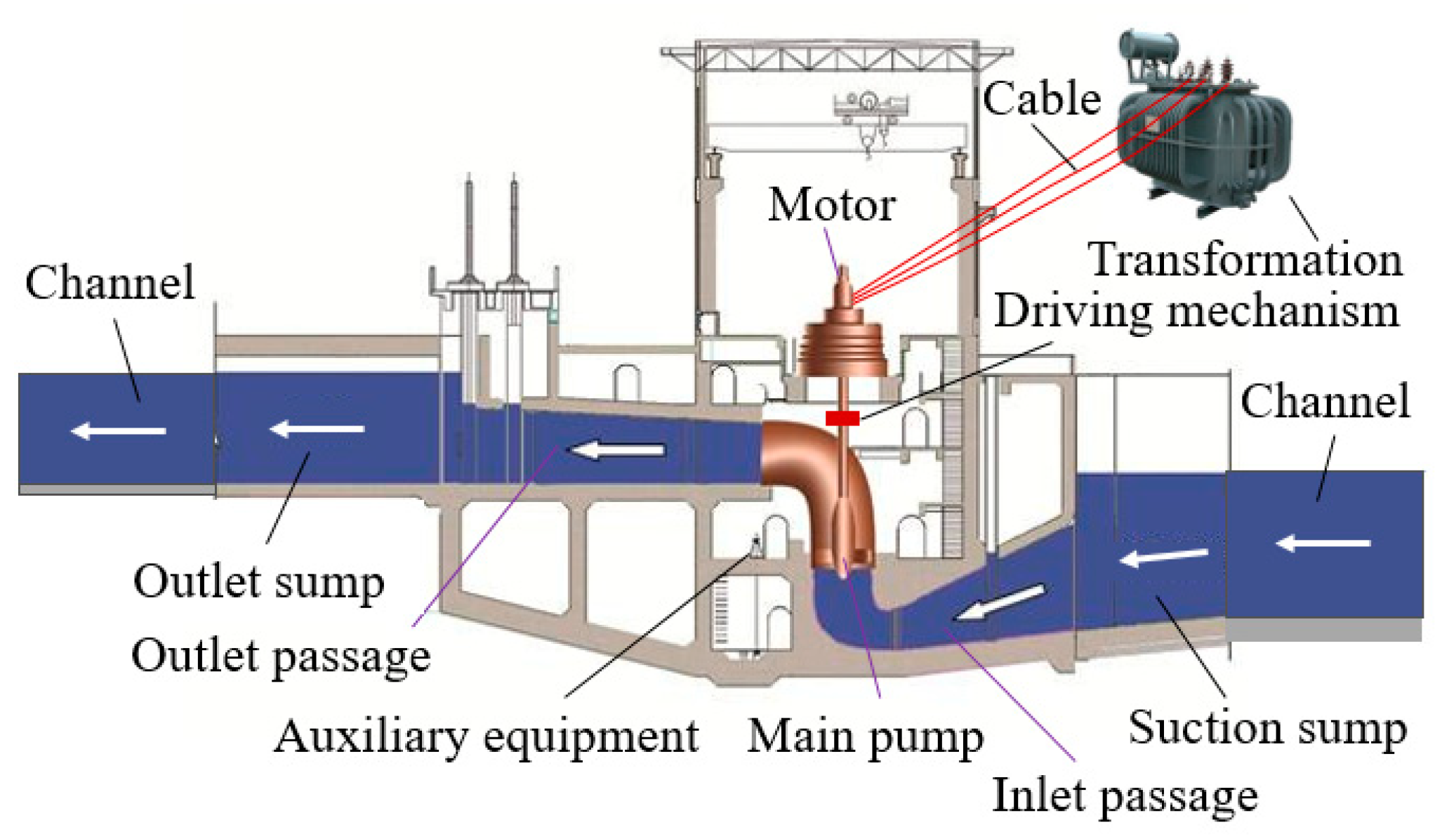
Pumping stations play a key role in agricultural irrigation and drainage, urban domestic water supply and sewage, industrial water supply and drainage, and ecological environment construction, and they have high energy costs. For a large open-channel water transfer system with pumping stations, power transmission facilities, pumping stations and water passing facilities are necessary to work together to transfer water from the source to the destination, and they are responsible for power transmission, energy conversion and water transport. During this process, energy loss is inevitable. Energy wasting equipment and water passing facilities include main water pumps, electrical motors, drive mechanisms, inlet and outlet passages and their accessories, suction and outlet sumps. In addition, power transmission, power transformation, and auxiliary equipment must also assist in the function of main pump units (see Figure 1). Water transfer performance of the open-channel is interrelated with pump operation performance. Therefore, it is important to study operation optimization methods for an open-channel water transfer system to decrease energy consumption and improve energy savings.
Previous studies on optimization mainly focused on improving the efficiency of a single pump by adjusting pump blade angles, pump rotational speed or valve opening based on the varying head. Then, the goal expanded to developing high-efficiency pump assemblies (composed of the main pump, inlet passage and outlet passage) and pumping stations (considering main pumps, inlet passages, outlet passages, matching motors, driving mechanisms, a suction sump and an outlet sump). The focus has since shifted to lowering the power consumption and energy costs of pumping stations or a complex water transfer system entirely.
Many researchers have studied the operation optimization theories for water transfer pumping station systems. Olszewski [1] investigated optimal operation for parallel pumps in a pumping system using the genetic algorithm, and regulated operation modes by adjusting valve opening, throttling and frequency conversion, aiming to achieve minimal power consumption, flow rate balance and maximum total efficiency. Feng et al. [2] discussed the optimal operation of main pump units using the genetic algorithm, giving electricity cost savings of 4.73−31.27% in the schemes of adjusting blade angles and time-varying electrical price. Abkenar et al. [3] established multiple objective nonlinear optimizing models for a water diversion system, considering the cost and energy consumption of environmental contamination emissions, and determined optimization schemes by applying the genetic algorithm with continuous and discrete coding. Ramos et al. [4] studied the optimal operation of a water supply system in which the turbine generation and wind turbine afforded power for pumping stations, and the energy efficiency and hydraulic efficiency of the system were improved. Bohórquez et al. [5] applied genetic algorithm (GA) to a water distribution system using EPANET software, allowing for 26% and 50% of energy cost and leakage reduction in the case of unique speed pumps, and 33% and 55% of that in the case of variable speed pumps. Zhang et al. [6] utilized a neural network algorithm to model pump energy consumption and proposed an artificial immune network to schedule the model, achieving energy savings of 6–14%. Zhuan et al. [7] proposed an extended reduced dynamic programming algorithm to solve the optimal operation scheduling of a pumping station with multiple pumps, and the results indicated the feasibility of reducing operation energy and maintenance costs with this method. Naoum-Sawaya et al. [8] applied the simulation optimization method to study the optimal operation of pumps in water supply networks, ensuring the lowest operating cost and the least amount of seepage. Bagirov et al. [9] put forward a novel approach for modelling explicit pump scheduling to minimize energy consumption that was based on the combination of the grid search with the Hooke–Jeeves pattern search method. Ghaddar et al. [10] presented a Lagrangian decomposition approach for pump scheduling in water networks, and the results illustrate significant costs savings. Charles and Bauer [11] optimized the operation of cascade pumping stations considering river water loss. Zhang and Zhuan [12] investigated the operation optimization problem of the third Huaiyin pumping station to save on electricity while satisfying the required flow demand; the results indicate that the operational electricity tariff is reduced by 7.71% by the improved dynamic programming algorithm in comparison with the benchmark scheduling. Gong and Cheng [13] reported a method for optimizing the operation of cascade pumping stations based on the head decomposition–dynamic programming aggregation method considering water level requirements. Zhao and Feng [14] reported an evaluation strategy of particle swarm optimization to achieve the optimal operation of a pumping station system. Liu et al. [15] proposed an improved self-adaptive grey wolf optimization (IAGWO) to solve the operation problems of cascaded pumping stations. Compared to the present scheme, the schemes employing IAGWO, adaptive grey wolf optimization (AGWO), grey wolf optimization (GWO) and particle swarm optimization (PSO) could save 0.80268%, 0.80189%, 0.77369% and 0.45331% of daily operating expenses, respectively. Zhuan et al. [16] studied operation optimization of the fourth Huai’an stations of the east route of the South-to-North Water Transfer Project and proposed a decomposition method to solve the model; the result of which was 2.54% energy saving compared with the benchmark scheduling scheme. Zhang et al. [17] optimized the scheduling of cascade pumping stations in an open-channel water transfer systems based on station skipping. Turci et al. [18] reported two adaptive and one improved multi-population-based nature-inspired optimization algorithms for water pump station scheduling, comparing it with GA, PSO and ant colony optimization (ACO) to show its better performance. Dong and Yang [19] proposed a data-driven model to carry out the operation optimization scheduling of water diversion and drainage pumping stations in the presence of complex hydrometeorological constraints. The results clearly confirm its effectiveness and improved economic performance compared to the existing benchmark solution. Parvez et al. [20] reviewed the prior research work for hydro-scheduling by considering various constraints, different solutions and modelling techniques. Cimorelli et al. [21] reported that a well-designed GA is capable of tackling optimal pump scheduling. In addition, a new decision-variable representation was proposed, specifically suited to parallel pump systems.
In the contemporary research, the pump assembly (only composed of a pump and inlet and outlet passages) or pump unit (only composed of a pump, motor and driving device) is taken as the study subject, and energy loss of other equipment or facilities is partly considered in some studies. For example, water quantity loss is considered in the literature [5,11]. In short, optimization methods were focused on in previous research, and energy consumption or cost in models were considered incomplete factors. Thus, energy savings could be further improved.
The goal of this study is to present a methodology for improving energy saving by optimizing the operation strategies of pumping stations, targeting parallel pumping stations in an open-channel water transfer system with double lines that transfers water from the Sanjiangying intake of the Yangtze River to the Huai’an pumping station in the eastern route of South-to-North Water Transfer Project in China. The novelty of this study is that energy consumption is considered more comprehensively than in previous work. The energy consumption includes not only the power of main electrical motors in the pumping stations but also the power of auxiliary equipment (including water supply pumps, water drainage pumps, fans and so on) for main pumps, power transmission and transformation equipment, and hydraulic and water quantity losses (including evaporation and leakage) of the channel. Using this approach, computation load and time would be increased greatly by repeated iterations of flow rate and channel water level. An efficient methodology is presented in which the dichotomy approach is employed to optimize the flow rate distribution of double water lines to determine the head and flow rate of each pumping station; simulated annealing-particle swarm optimization is implemented to optimize power consumption in pumping stations. This paper presents data verifying that the proposed method is more time efficient than double-layer simulated annealing–particle swarm optimization (dSA–PSO), and yields higher energy savings than the benchmark operation strategy for pumping stations.
2. Description of Parallel Pumping Stations in an Open-Channel System
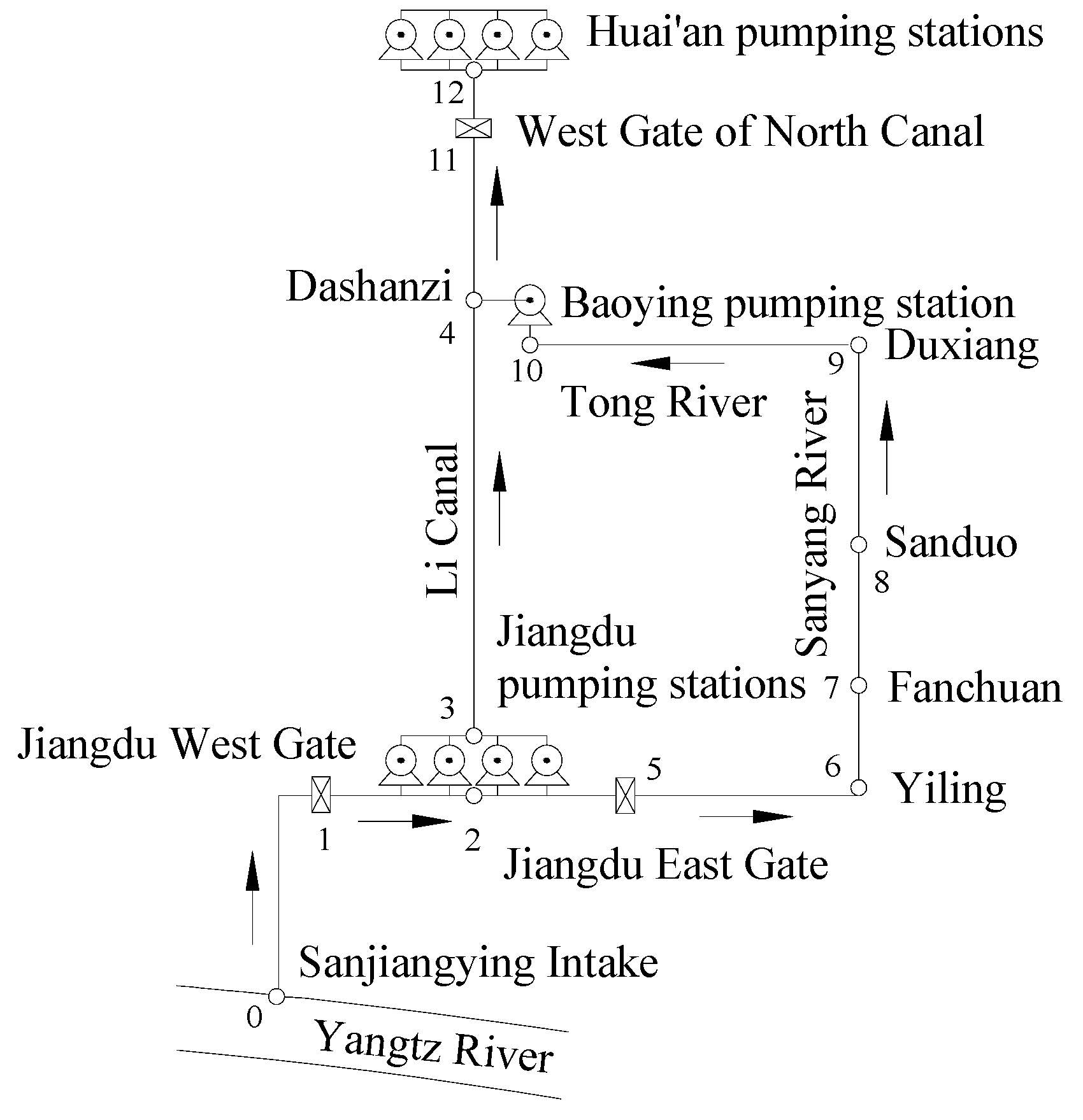
The South-to-North Water Diversion Project is a large-scale interbasin water transfer project in China. Water is transferred from the Yangtze River in southern China to the more arid northern regions through eastern, middle and western routes. In the eastern route project, 13 stages, including 34 pumping stations, are located along the double open-channel water conveyance lines. The first-stage of the eastern route project is combined with the 1st, 2nd, 3rd, 4th Jiangdu pumping station and the Baoying pumping station, power transmission and transformation equipment, and the water transferring open-channel. The water transfer diagram is shown in Figure 2.
In Figure 2, the arrows represent flow direction, and the numbers are the compute nodes. The water flows from the Sanjiangying intake (source) in the Yangtz River to the Jiangdu West Gate, after which point some water is pumped by the Jiangdu pumping stations and flows to Dashanzi along the Li Canal continuously, while some flows from the Jiangdu West Gate to the Baoying pumping station, passing by the Jiangdu East Gate along the Sanyang River and the Tong River. The two flows meet at Dashanzi, after which the water flows along the Li Canal to the downstream of the Huai’an pumping stations in the second stage of the eastern route project, passing by the West Gate of North Canal.
Table 1 shows the channel parameters, where evaporation is the long-term month mean value, which is related to temperature, air relative humidity, and wind speed, among other factors.
In the 1st, 2nd, 3rd, 4th Jiangdu pumping stations and the Baoying pumping station, there are 8, 8, 10, 7 and 4 axial flow pump units installed, respectively. The pump types are 1.75ZLQ-7, 1.75ZLQ-7, 2000ZLQ13.5-7.8, 2900ZLQ30-7.8, and 3500HDQ34-7.6, with rated power of 1000, 1000, 1600, 3400 and 3400 kW, respectively. The 1st, 2nd and 3rd Jiangdu pumping station share one 40,000 kVA transformer, and the others use one transformer separately. From the power substation to the transformer, the power transmission cable length is approximately 7 km for the Jiangdu pumping stations, and 27 km for the Baoying pumping station, with 110 kV voltage. The cable lengths from the transformer to electric motors are about 231, 251, 220, 462 and 20 m, and the voltage is 6 kV for the Jiangdu pumping stations and 10 kV for the Baoying pumping station.
Auxiliary equipment is installed in each pumping station. For instance, in-station water supply pumps are installed for cooling and lubrication. In-station water drainage pumps are used for draining water in the collecting gallery of the pump house during running, non-running and overhauling. Fans reduce heat generated from motors and solar radiation. Trash-removal equipment is installed to prevent trash from entering the main pumps.
3. Mathematical Model
3.1. Objective Function
For large parallel pumping stations in an open-channel water transfer system, power is transmitted from an external substation to the main transformer of pumping stations through cables and is continuously provided to the main motors and auxiliary equipment. A portion of the power is transformed into useful power, while the remainder is wasted due to power transmission, transformer, motor, driving mechanism, main pump, inlet and outlet passage, inlet and outlet sump, auxiliary equipment consumption, and water transfer losses. As shown in Figure 1, given the source water level zsjy of the Sanjiangying intake in the Yangtze River, the downstream level zha and the flow rate Qha of the Huai’an pumping stations (destination), the following mathematical model can be used for minimizing system input power P (kW) based on the order of energy transfer:
where i is the sequence number of pumping stations and i = 1, 2, 3, 4 and 5 represent the 1st, 2nd, 3rd, 4th Jiangdu pumping stations and the Baoying pumping station; ρ is the density of water, kg/m3; g is the acceleration of gravity, m/s2; Q is flow rate of single pump, m3/s; Hz is pump assembly head, m; n is the number of running pump units; ηz is pump assembly efficiency; ηdr is the driving efficiency (for direct driving, ηdr = 1.0); ηmot is electrical motor efficiency, ηmot = ηmot (γ), where γ is motor load coefficient; Pzn is input power of auxiliary equipment system, kW; ΔPte is energy loss of power transmission, kW; and ΔPb is energy loss of power transformation, kW.
In Equation (1), the input power of auxiliary equipment system Pzn mainly includes the consumption of the water supply and drainage, motor ventilation, trash removal, and lighting systems as well as the in-station transformer, which provides power to the main pump units. Input power can be calculated according to the actual operation system.
Transmission energy loss is related to transmission current, cable length and cable parameters. Assuming the input power of the electrical equipment that is connected with the end of the transmission cable is Ps (kW), the total current Ite through the cable can be obtained as:
where Ite is the total current, A; Ue is the voltage, kV; and cosφ is the power factor.
Transmission loss ΔPte can be obtained as:
where m is the number of cables; r0 is resistance per unit length of cable, Ω/km; and l is the length of the cable, km.
The energy loss of a main transformer ΔPb is related to its parameters and actual operation load. The operation load depends on the consumption of main pump units and other equipment. Energy loss of a transformer can be expressed as:
where Pkz is no-load comprehensive loss, kW, Pkz = P0 + eQ0; Pfz is rated load comprehensive loss, kW, Pfz = Pf + eQf; S is actual load capacity of the transformer, kVA; Sr is rated capacity of the transformer, kVA; P0 is no-load active loss, kW; Pf is load loss, kW; Q0 is no-load reactive loss, kvar, Q0 = I0%Sr × 10−2; Qf is short circuit reactive loss, kvar, Qf = Uf%Sr × 10−2; I0% is no-load current; Uf% is short circuit impedance; and e is reactive economy equivalent, kW/kvar, typically 0.01.
3.2. Constraint Conditions
The objective function should meet the flow rate, water level, and pump unit constraints.
3.2.1. Flow Rate Constraints
The required flow rate Qha of a water transfer destination is a given value of C1:
The flow rate Qw(x) of a different channel section x–x should be no more than the maximum allowable value Qw, max(x):
Considering the inevitable flow rate loss of leakage qs, evaporation qz, and the intake flow rate qf supplying to users along the channel, the flow rate should meet the continuity equation defined below:
where qsj, qzj, and qfj (j = 1, 2, …, 8) are water leakage, evaporation loss, and intake flow rate of the channel from the destination to the source. Water surface evaporation is related to temperature, air relative humidity, and wind velocity. Leakage loss is determined by the channel geometrical dimensions, roughness coefficient, ground water level, and soil permeability. According to the project original plan, the intake flows qfj (j = 2, 4, 5, 8) of Dashanzi, Sanduo, Fanchuan and Yiling are 50, 50, 150, and 250 m3/s, respectively, and qfj = 0(j = 1, 3, 6, 7). Qdsz, Qdx, Qsd, Qfc, Qyl, Qjdwg, and Qsjy are the flow rate of Dashanzi, Duxiang, Sanduo, Fanchuan, Yiling, Jiangdu West Gate, and Sanjiangying, respectively.
3.2.2. Water Level Constraints
The source water level zsjy and the destination water level zha are the given values of C2 and C3:
To ensure the safe operation of the channel, the water level z(x) at a different cross-section x–x should be subjected to the constraint zmin(x) and zmax(x):
According to the principle of energy conservation, the following energy equation can be derived at an open flow segment, supposing the upstream cross-section is u–u and the downstream cross-section is d–d:
where Qu and Qd are the flow rate on the cross-sections u–u and d–d, m3/s; zu and zd represent the potential energy per unit weight of liquid on the u–u and d–d cross-sections, typically to the point on the water surface, m; pu and pd are the pressure measurements at the water surface on cross-section u–u and d–d, N/m2, pu = pd = 0; vu and vd are mean velocity on cross-section u–u and d–d, m/s, vu = Qu/Au, vd = Qd/Ad; Au and Ad are the area on cross-sections u–u and d–d, m2; αu and αu are kinetic energy correction coefficient on cross-sections u–u and d–d, (for the gradient flow section, they are 1.05–1.10); and ΔPH, ΔPL and ΔPV are respectively the energy losses caused by lengthwise hydraulic, leakage, and evaporation losses, W.
According to Equations (6) and (3), given zha, Qha and zsjy, we can obtain the water level and flow rate at each cross-section. Supposing zjdu, zjdd, zbyd, and zdsz are downstream and upstream water levels of the Jiangdu pumping stations, the downstream water level of the Baoying pumping station, and the water level of Dashanzi, the following water level balance conditions should be satisfied:
3.2.3. Head Constraint
According to the theoretical performance and the operation data of the pump units in practice, the allowable operation head is determined as follows:
3.2.4. Blade Angle Constraint
For blade angle full adjustable pumps, the pump blade angles β should meet the following constraints:
3.2.5. Flow Rate Constraint
For a given pump assembly head Hz, there is a one-to-one correspondence between the pump blade angle and flow rate; the flow rate should obey maximum and minimum constraints:
3.2.6. Single Pump Unit Power Constraint
For an electrical motor, the input power should be no more than the maximum value Pmax to avoid operation overload:
3.2.7. Pump Number Constraint
The quantity of operating pump unit n in the pumping station should be no more than the quantity M of machines installed in the pumping station:
4. Solution Methods
4.1. Optimization Algorithm
4.1.1. Dichotomy Approach
The dichotomy approach (abbreviating as DA) is a commonly used computational method that introduces the dichotomy into the approaching iterative search as follows:
- (1)
- For variable x ∈ [a, b], divide the definitional domain into n equal parts.
- (2)
- For interval step Δx = (b − a)/n, xi = a + iΔx (I = 0, 1, 2, …, n).
- (3)
- Calculate the values of function f(xi) and obtain the minimum fmin(xi).
- (4)
- If the minimum value locates boundary point xi (I = 0 or n), take the midpoint of the boundary domain and calculate its function value, compare it with the current minimum value, and identify the points x* with the minimum function value. Otherwise, take the midpoint x′ = (xi−1 + xi)/2 and x″ =(xi + xi+1)/2 of interval [xi−1, xi] and [xi, xi+1] respectively, then calculate f(x′) and f(x″), and compare them with f(xi) to get the minimum points x*.
- (5)
- Shorten the search interval by half and determine the minimum point among f(x*), f(x* − Δx/2) and f(x* + Δx/2).
- (6)
- Shorten the search interval again by half, and stop calculations once the precision is satisfied.
4.1.2. Simulated Annealing–Particle Swarm Optimization
Particle swarm optimization (abbreviating as PSO) is an evolutionary stochastic swarm computational technique that is based on swarm movement and intelligence [22]. In the algorithm, a group of random particles is initialized, and the optimal solution is obtained by iterations. Each particle adjusts its position and velocity based on both its own experience and that of neighboring particles. At the end of each iteration, all particles observe the objective function value and move toward better positions. The velocity and position of each particle j in iteration t + 1 can be computed as follows [23,24,25]:
where j represents the jth particle; w is inertial weight; c1 and c2 are study factors; r1 and r2 are two independent random numbers between 0 and 1; vj is the velocity of particle j; xj is the position of particle j; pj is the best experience of particle j; and pg is the best experience of the all particles.
Simulated annealing (abbreviating as SA) is based on the physical annealing process of solid matter [26]. In this algorithm, for a minimum function f(x), x is a current solution, and x′ is a new solution generated in the neighbourhood domain randomly, supposing ΔE = f(x′) − f(x). Then, x is substituted with x′ at a probability pa = min{1, exp(−ΔE/T)}, where T is temperature. When f(x′) < f(x), pa = 1, which implies that the better solution is accepted with probability 1; otherwise, pa is a value between 0 and 1. The algorithm accepts a bad and new solution at a certain probability.
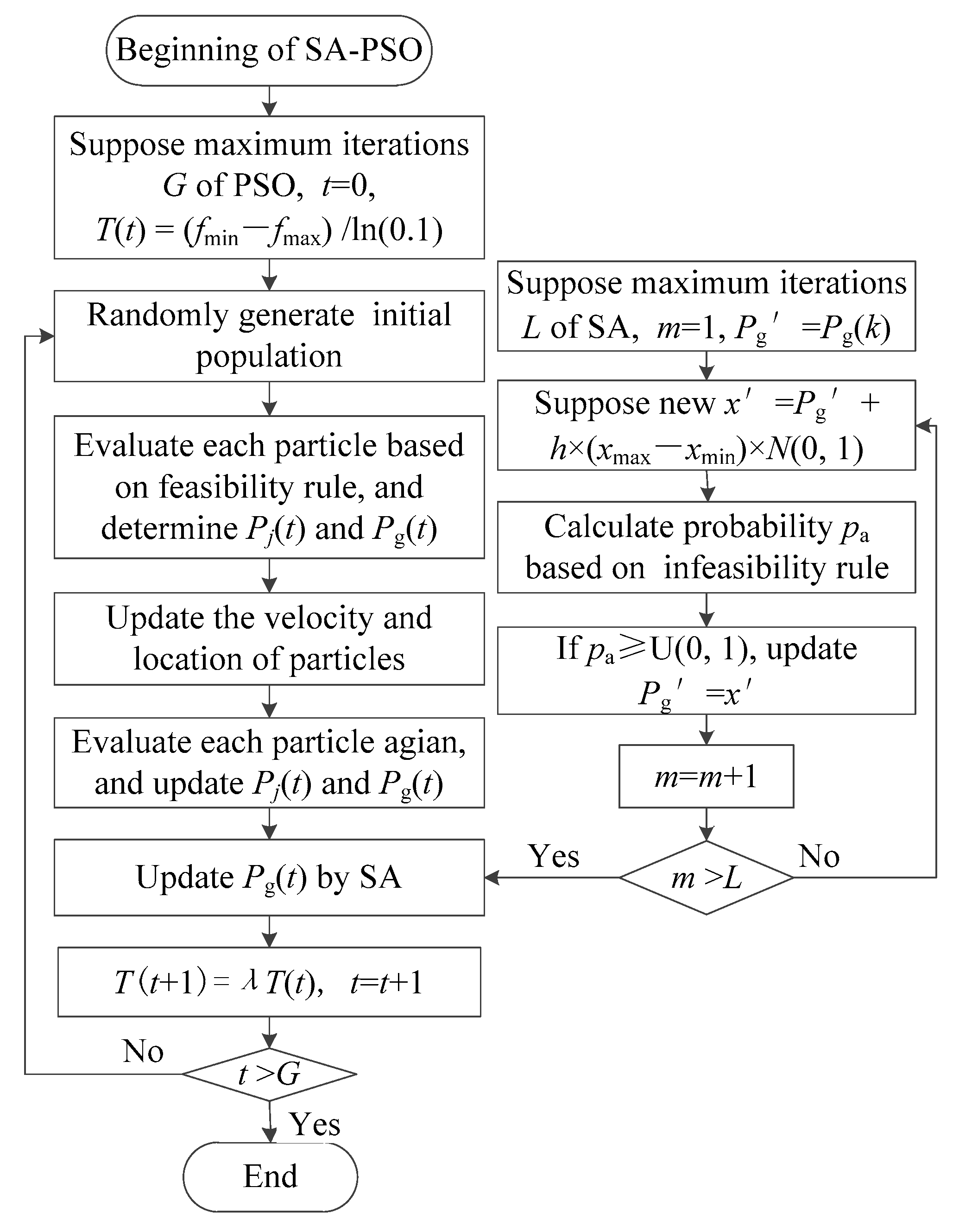
Simulated annealing–particle swarm optimization (abbreviating as SA–PSO) introduces SA to the particle velocity and position update process to avoid falling into the local extreme value area and to obtain the global optimal solution. SA-PSO is simple and easy to implement, and it improves PSO performance [27,28].
The feasibility rule can be used to address equality and inequality constraints. It can help the SA jump out of the local minimum and update the best position of the particle and the best position of the population. For general constrained optimization problems,
where gj is constraints of inequality; hk is constraints of equality; and xi is decision variable.
F = Min f(x)
Define the infeasibility degree φ of a solution xi as follows:
The infeasibility degree is the distance from the solution xi to the feasible region. The further away from the feasible region, the greater the infeasible degree, and vice versa. If xi is feasible, the infeasibility degree is zero. The feasibility rule is as follows: (1) the feasible solution is always superior to the infeasible one; (2) if both solutions are feasible, the solution with a good target value is superior; and (3) if both solutions are infeasible, the solution with a lower infeasibility degree is superior.
The schematic diagram of SA-PSO is shown in Figure 3, where T is the temperature, λ is annealing rate, h is searching step (h = 0.01 in this study), N(0,1) and U(0,1) are random numbers between 0 and 1, and xmax and xmin are upper and lower bounds of the search variable.
4.2. Solving Process
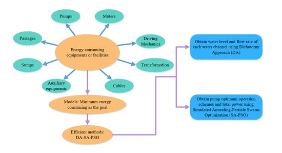
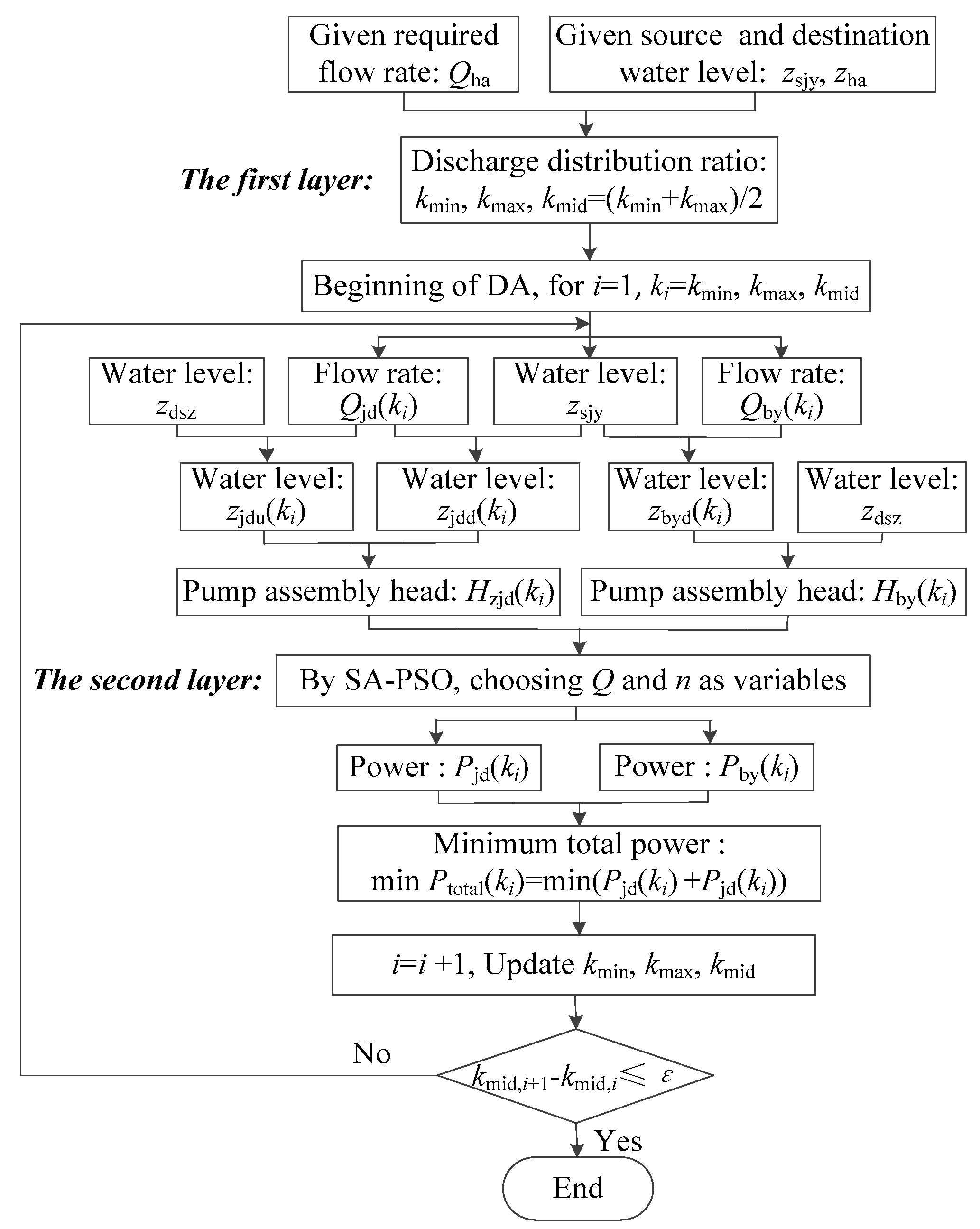
The mathematical model is a nonlinear optimization problem with equality and inequality constraints. In the model above, pump assembly head Hz is the difference between downstream and upstream water level of the pumping station (see Equation (11)), and the water level is related to the flowrate of each water channel. Flow rate Q of a single pump and the number of running pumps n could be determined according to the pump assembly head and the flow rate of the water channel. The mathematical model could be decomposed into two layers. In the first layer, discharge distribution ratio is chosen as a variable, and the water level and flow rate of the channel are determined to obtain the flow rate and head of pumping stations by DA. In the second layer, the flow rate (or blade angles) and the number of running pumps of each type are regarding as variables. In our previous study, we analyzed the application of GA, PSO, and SA–PSO to optimize pumping station operations. The results indicated that SA–PSO had better search ability [29]. SA–PSO is used to solve the second layer here. The combination of DA and SA–PSO is called DA–SA–PSO. The schematic diagram of the hybrid algorithm of the model is shown in Figure 4.
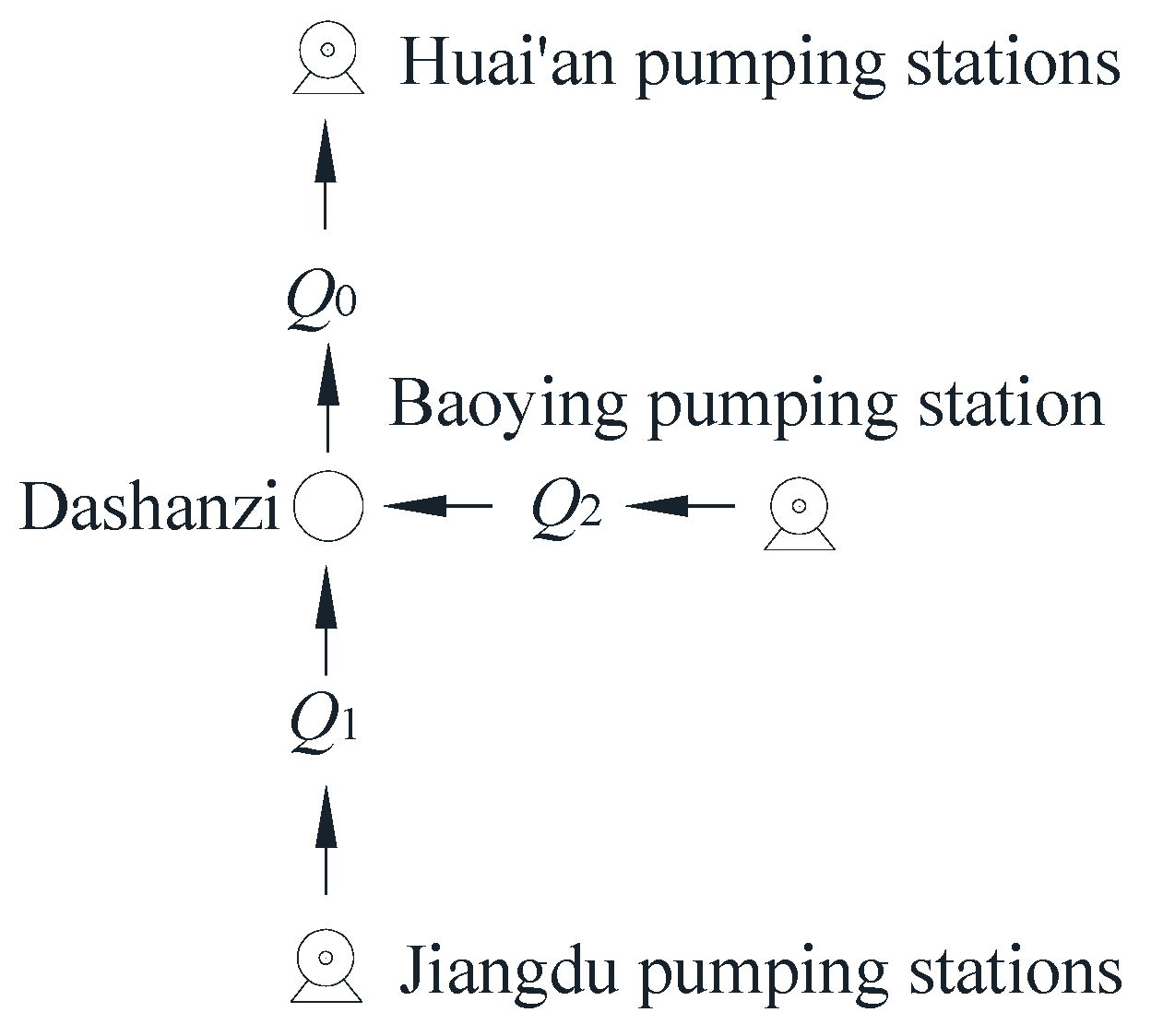
Specifically, in the first layer, the water transfer destination is the Huai’an pumping station. Given the required discharge Qha, the water level zha of the destination and related parameters of the channel, the water level and flow rate along the channel could be calculated backwards to determine the pump assembly head. After converging at Dashanzi of the Li Canal from the Jiangdu pumping stations and the Baoying pumping station, the water is transferred to the Huai’an pumping stations. Supposing the flow rate is Q0 of Dashanzi after water convergence and is Q1 before water convergence from the Jiangdu pumping stations, the flow rate of the Baoying pumping station is Q2 = Q0 − Q1 (see Figure 5). The discharge distribution ratio is defined as k = Q1/Q0, where k ∈ [0,1], which is a unique variable determining the water level and flow rate. They could be calculated by DA. The influences of discharge distribution ratio k on input power are analyzed. When the system input power lowest, the discharge distribution ratio is the optimal kopt.
The water level of Dashanzi zdsz and the flow rate Q0 can be obtained by Equation (10) based on the given water level zha and required flow rate Qha. For any reasonable discharge distribution ratio k (the flow rate of the pumping station should be between the maximum and minimum to guarantee normal operation), according to Q1 = k·Q0 and Q2 = Q0 − Q1, the flow rate Qby (namely Q2) and upstream water level zbyu (namely zdsz, ignoring the loss along from the Baoying pumping station to Dashanzi) of the Baoying pumping station can be determined. The flow rate Qjd and upstream water level zjdu of the Jiangdu pumping stations can also be obtained. Similarly, given the source water level zsjy, the downstream water level zjdd of the Jiangdu pumping stations and zbyd of the Baoying pumping station can be obtained based on the above Qby and Qjd. As a result, the pump assembly head could be calculated by Equation (11).
In the second layer, according to the pump assembly head obtained by the first layer, the flow rate of a single pump and the number of running pumps are selected as variables, and the SA–PSO algorithm is used to determine operation schemes and power. The related parameters of SA–PSO are as follows: the population size is 200, the maximum number of iterations is 300, the inertia weight is varied by Equation (21), the annealing rate is 0.92, and the searching step is 0.01.
where wmax and wmin are the maximum and minimum inertia weight with values of 1.5 and 0.01, respectively; and f, favg and fmin are current, average and minimum fitness function, respectively.
5. Results and Analysis
When zha is 6.0 m and Qha is 300, 200, and 100 m3/s, system operation schemes of different discharge distribution ratio are determined at different zsjy such as 3.00, 2.19, and 1.40 m.
The downstream water level zbyd of the Baoying pumping station is related closely to water level and flow rate of Sanjiangying. Considering the navigation requirements of the Sanyang River and the Tong River, zbyd is limited between 0 and 2.60 m.
The maximum flow rate of the Baoying pumping station is 150 m3/s based on the pump assembly performance. Given the 300, 200, and 100 m3/s flow rate of the Huai’an pumping stations, the corresponding minimum discharge distribution ratio is 0.5, 0.25, and 0, respectively. The flow rate of the Sanyang River and the Tong River has more influences on hydraulic loss than that of the Li Canal. The hydraulic loss is positively correlated with the flow rate, so the flow rate of the Sanyang River and the Tong River is limited. In the range of 1.0–3.5 m of source water level, considering the demanding water level of the Baoying pumping station downstream, feasible ranges of the discharge distribution ratio could be calculated. In this study, the calculation accuracy of discharge distribution ratio k is 0.01.
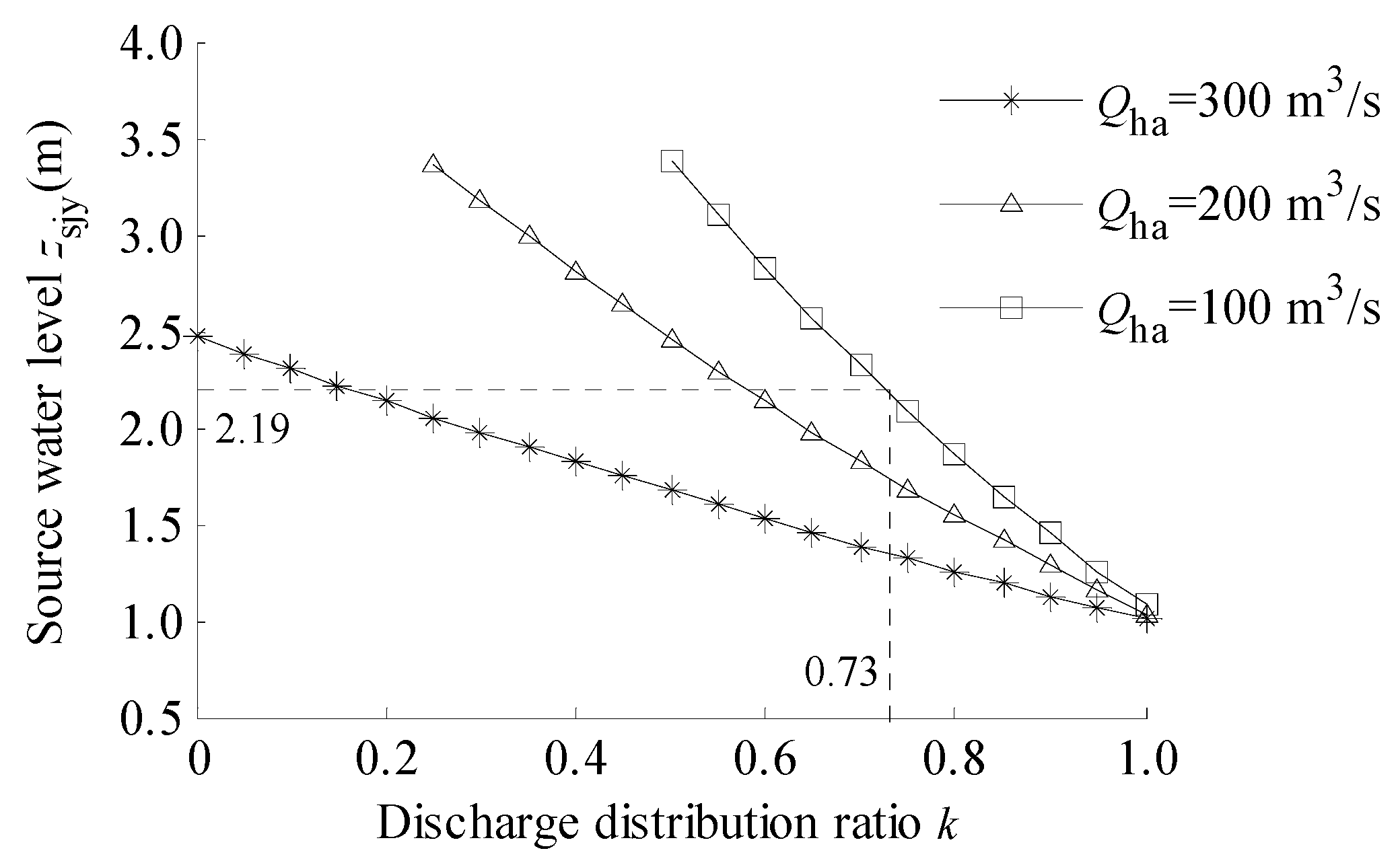
Figure 6 shows the relations between the source water level zsjy and the discharge distribution ratio k under the water level constraints. Taking Qha = 300 m3/s as a case, when zsjy is 2.19 m, we can see that the feasible interval of k is [0.73, 1.0]. According to Figure 5, in the range of 1.0–3.5 m of source water level, the feasible interval of flow distribution ratio corresponding to any source water level can be determined, and the results are listed in Table 2.
The pump cannot operate normally if the flow rate is too high or low. The flow rate of a single pump unit in the Baoying pumping station is subjected to maximum and minimum values, k ∉ [0.83, 1.0). Under the constraints of water level and flow rate, k ∈ [0.73, 0.82] ∪ {1.0}, where k ∈ {1.0} represents that none of pumps runs in the Baoying pumping station, and the flowrate is zero. For different zsjy and Qha, the feasible interval of k can be determined in the same manner, and the results are listed in Table 3.
In calculation, k is varied approaching the optimal value by the DA algorithm. Figure 7 shows the relation between discharge distribution ratio k and system input power P for different zsjy and Qha, and the optimal discharge distribution ratios kopt are listed in Table 4. From the above results, at a given flow rate of the Huai’an pumping stations, when the source water level is raised, the feasible intervals of discharge distribution ratio are enlarged, and the system input power and optimal discharge distribution ratio are decreased. At a given source water level, when the required flow rate of the Huai’an pumping stations is decreased, the system input power and optimal discharge distribution ratio decrease as well, but the feasible intervals of discharge distribution ratio are increased.
Table 5 and Table 6 show water level of compute nodes and optimized results of pump units with the optimal discharge distribution ratio. In Table 5, “—” represents the pump unit does not run. The operation scheme of the 3rd Jiangdu pumping station is not listed because this station does not need to run (i.e., its flow rate is zero). The total computation time using DA−SA−PSO is approximately 20 min. A decision within 30 min is regarded as real time for an open-channel water transfer system.
For a given zsjy, the pump assembly head increases with an increase in flow rate to meet the requirements due to the hydraulic loss increases. The pump assembly head of the Baoying pumping station is higher than that of the Jiangdu pumping stations, which indicates that the hydraulic loss of the channel starting from the Sanyang River and the Tong River to the Baoying pumping station downstream is larger than that of the channel starting from the Jiangdu pumping station to Dashanzi along the Li Canal.
The optimal discharge distribution ratio increases with flow rate increment of the Huai’an pumping stations. For a given flow rate of the Huai’an pumping stations, the pump assembly head and optimal discharge distribution ratio decrease with an increase in source water level. Namely, the flow rate of the Jiangdu pumping stations decreases, while that of the Baoying pumping station increases. This is because the pump assembly head decreases with an increase in source water level, and the efficiency increment of the Jiangdu pumping stations is more than that of the Baoying pumping station.
Meanwhile, with an increase in source water level, the source flow rate increases to less than 0.1%, which could be regarded as an invariant. One possible reason is that the depth of the channel and wetted perimeter increase, but the water flows slowly, resulting in slightly increased loss from water leakage. The operation characteristics of pumping stations exhibit close relationships with water level and flow rate.
For the South-to-North Water Transfer Project, the original flow rates of the Jiangdu pumping stations and the Baoying pumping station are 400 m3/s and 100 m3/s, and the discharge distribution ratio k is 0.8. The input power of the optimal and original discharge distribution ratio is listed in Table 7, where “—” represents the system could not operate normally under original discharge distribution. From the table, the input power could be saved by 0.2–2% using the optimal solution.
An explanation is that in the scheme of original discharge distribution ratio, flow rate (or blade angles) and the number of running pumps of each type are optimized using SA−PSO. In actuality, the pumping stations operate according to managerial experience with a lack of scientific guidance. Under a given water level and required flowrate, the pump blade angles are regulated to a fixed value (which is usually is 0°), and the pump assembly with high efficiency is preferred to be operated. For the case in this study, the pump unit operation schemes and input power are calculated under the assumption that the pump blade angles are all 0°, as shown in Table 8. Due to the constraints of fixed blade angles and the integer number of running pumps, the total flow rate may be greater than what is required, resulting in flow rate waste and a great increase in input power. Compared with Table 8, the input power of optimal discharge distribution ratio is saved by 14–35% in Table 7.
The mathematical model could also be solved by double-layer SA−PSO (dSA−PSO). The optimal discharge distribution k is regarded as a variable in the first layer and is determined by SA−PSO, where the population size is 20, the maximum number of iterations is 30, and the other parameters are the same those listed above. The calculating amount is quite large, with a long computation time of approximately 10 h. Good solutions could be obtained by the two methods, and the results are shown in Table 9.
The results indicate that the accuracy of discharge distribution ratio is higher, and the input power is approximately 0.067% lower by dSA−PSO than that by DA−SA−PSO, while the difference of kopt is approximately 0.5% between the two methods. The computation time is only approximately 20 min by DA−SA−PSO, which is 1/30 of that by dSA−PSO, because repeated iterations of water level and flow rate are avoided. Therefore, the DA−SA−PSO algorithm exhibits more advantages in terms of calculation amount and speed, and is efficient for obtaining optimal solutions in real time according to frequently varying water levels of the source or destination, required flow rate, or technical equipment conditions for parallel pumping stations in an open-channel water transfer system with double water lines. The dSA−PSO is useful for calculating optimal solutions in advance, lessening the impact of time restrictions. The solutions could be stored digitally and used based on different conditions.
For a more complex water diversion system, such as three or more water diversion lines and more pumping stations, the modelling method and solving process are similar to above. The difference is the increasing number of variables, working load and computation time.
6. Conclusions
This paper proposes an efficient methodology for optimizing energy use of parallel pumping stations in an open-channel water transfer system with double water lines. The energy consumption includes the power of main electrical motors and auxiliary equipment, and power transmission, transformation equipment, hydraulic, and water volume losses. To avoid repeat iterations of flow rate and water level of the channel, the DA was applied to optimize the flow rate distribution of double water lines to determine the head and flow rate of each pumping station, and SA-PSO was implemented to optimize power consumption in pumping stations. The following conclusions can be obtained:
(1) Using the hybrid DA−SA−PSO, the calculation time is 1/30 of dSA−PSO. Compared with the original scheme, the system input power of the schemes with optimal discharge distribution could save 14%–35% of energy. DA−SA−PSO is useful for solving optimization problems in real time considering frequently varying conditions.
(2) When the flow rate of the transfer destination is a given value, such as 300, 200 and 100 m3/s, the feasible range of discharge distribution ratio is enlarged with the increase in source water level, and the pump assembly head, optimal discharge distribution ratio, and system operation power are decreased. When the source water level is a given value, such as 3.00, 2.19 or 1.40 m, the feasible range of discharge distribution ratio is shortened with the increasing flow rate of the destination, and the optimal discharge distribution ratio, pump assembly head and system input power are all increased. The operation characteristics of pumping stations are relevant to the water lever and flow rate.
(3) For complex systems with more water transfer lines and pumping station stages, the modelling method and solving process could also be applied.
Author Contributions
All authors contributed in the preparation of this manuscript. Conceptualization, X.F. and B.Q.; methodology, X.F., B.Q. and Y.W.; software, X.F. and Y.W.; validation, X.F. and B.Q.; formal analysis, X.F. and B.Q.; investigation, X.F. and Y.W.; resources, X.F.; data curation, X.F.; writing—original draft preparation, X.F.; writing—review and editing, B.Q. and Y.W.; funding acquisition, X.F. and B.Q. All authors have read and agreed to the published version of the manuscript.
Funding
This research was funded by National Natural Science Foundation of China No. 51509217 and No. 51679208.
Conflicts of Interest
The authors declare no conflict of interest.
References
- Olszewski, P. Genetic optimization and experimental verification of complex parallel pumping station with centrifugal pumps. Appl. Energy 2016, 178, 527–539. [Google Scholar] [CrossRef]
- Feng, X.L.; Qiu, B.Y.; Cao, H.H.; Wei, Q.L.; Teng, H.B. Optimal operation for Baoying Pumping Station in East Route Project of South-to-North Water Transfer. Chin. J. Mech. Eng. 2009, 22, 78–83. [Google Scholar] [CrossRef]
- Abkenar, S.M.S.; Stanley, S.D.; Miller, C.J.; Chase, D.V.; McElmurry, S.P. Evaluation of genetic algorithms using discrete and continuous methods for pump optimization of water distribution systems. Sustain. Comput. Inform. 2015, 8, 18–23. [Google Scholar]
- Ramos, H.M.; Kenov, K.N.; Vieira, F. Environmentally friendly hybrid solutions to improve the energy and hydraulic efficiency in water supply systems. Energy Sustain. Dev. 2011, 15, 436–442. [Google Scholar] [CrossRef]
- Bohórquez, J.; Saldarriaga, J.; Vallejo, D. Pumping pattern optimization in order to reduce WDS operation costs. Proc. Eng. 2015, 119, 1069–1077. [Google Scholar] [CrossRef] [Green Version]
- Zhang, Z.J.; Kusiak, A.; Zeng, Y.H.; Wei, X.P. Modeling and optimization of a wastewater pumping system with data-mining methods. Appl. Energy 2016, 164, 303–311. [Google Scholar] [CrossRef]
- Zhuan, X.T.; Xia, X.H. Optimal operation scheduling of a pumping station with multiple pumps. Appl. Energy 2013, 104, 250–257. [Google Scholar] [CrossRef]
- Naoum-Sawaya, J.; Ghaddar, B.; Arandia, E.; Eck, B. Simulation-optimization approaches for water pump scheduling and pipe replacement problems. Eur. J. Oper. Res. 2015, 246, 293–306. [Google Scholar] [CrossRef]
- Bagirov, A.M.; Barton, A.F.; Mala-Jetmarova, H.; Al Nuaimat, A.; Ahmed, S.T.; Sultanova, N.; Yearwood, J. An algorithm for minimization of pumping costs in water distribution systems using a novel approach to pump scheduling. Math. Comput. Model. 2013, 57, 873–886. [Google Scholar] [CrossRef]
- Ghaddar, B.; Naoum-Sawaya, J.; Kishimoto, A.; Taheri, N.; Eck, B. A Lagrangian decomposition approach for the pump scheduling problem in water networks. Eur. J. Oper. Res. 2015, 241, 490–501. [Google Scholar] [CrossRef]
- Charles, T.J.; Bauer, K. Transient control for a multiple booster pumping station and transmission pipeline system—Design, testing, adjustment, and operation. In Proceedings of the Pipelines Congress 2008-Pipeline Asset Management: Maximizing Performance of Our Pipeline Infrastructure, Atlanta, GA, USA, 22–27 July 2008; Volume 321, pp. 1–10. [Google Scholar]
- Zhang, L.; Zhuan, X.T. Optimization on the VFDs’ operation for pump units. Water Resour. Manag. 2019, 33, 355–368. [Google Scholar] [CrossRef]
- Gong, Y.; Cheng, J.L. Optimization of cascade pumping stations’ operations based on head decomposition–dynamic programming aggregation method considering water level requirements. J. Water Res. Plan. Manag. 2018, 144, 04018034. [Google Scholar] [CrossRef]
- Zhao, F.L.; Feng, X.L. Evaluation strategy of particle swarm optimization and it’s application in pumping station system optimal operation. In Proceedings of the 29th IAHR Symposium on Hydraulic Machinery and Systems, Kyoto, Japan, 16–21 September 2018. [Google Scholar]
- Liu, X.L.; Tian, Y.; Lei, X.H.; Wang, H.; Liu, Z.R.; Wang, J. An improved self-adaptive grey wolf optimizer for the daily optimal operation of cascade pumping stations. Appl. Soft Comput. 2019, 75, 473–493. [Google Scholar] [CrossRef]
- Zhuan, X.T.; Zhang, L.; Li, W.; Yang, F. Efficient operation of the fourth Huaian pumping station in east route of South-to-North Water Diversion Project. Int. J. Electr. Power 2018, 98, 399–408. [Google Scholar] [CrossRef]
- Zhang, Z.; Lei, X.H.; Tian, Y.; Wang, H.; Su, K.P. Optimized scheduling of cascade pumping stations in open-channel water transfer systems based on station skipping. J. Water Res. Plan. Manag. 2019, 145, 05019011. [Google Scholar] [CrossRef]
- Turci, L.O.; Wang, J.C.; Brahmia, I. Adaptive and improved multi-population based nature-inspired optimization algorithms for water pump station scheduling. Water Resour. Manag. 2020, 34, 2869–2885. [Google Scholar] [CrossRef]
- Dong, W.; Yang, Q. Data-driven solution for optimal pumping units scheduling of smart water conservancy. IEEE Internet Things J. 2020, 7, 1919–1926. [Google Scholar] [CrossRef]
- Parvez, I.; Shen, J.J.; Khan, M.; Cheng, C.T. Modeling and solution techniques used for hydro generation scheduling. Water 2019, 11, 1392. [Google Scholar] [CrossRef] [Green Version]
- Cimorelli, L.; D’Aniello, A.; Cozzolino, L. Boosting genetic algorithm performance in pump scheduling problems with a novel decision-variable representation. J. Water Res. Plan. Manag. 2020, 146, 04020023. [Google Scholar] [CrossRef]
- Eberhart, R.C.; Shi, Y. Comparing inertia weights and constriction factors in particle swarm optimization. In Proceedings of the 2000 Congress on Evolutionary Computation, La Jolla, CA, USA, 16–19 July 2000; Volume 1, pp. 84–88. [Google Scholar]
- Kennedy, J.; Eberhart, R. Particle swarm optimization. In Proceedings of the IEEE International Conference on Neural Networks, Perth, WA, Australia, 27 November–1 December 1995; pp. 1942–1948. [Google Scholar]
- Trelea, I.C. The particle swarm optimization algorithm. Inform. Process. Lett. 2003, 85, 317–325. [Google Scholar] [CrossRef]
- De Aragao, A.P.; Asano, P.T.L.; Rabelo, R.D.L. A Reservoir Operation Policy Using Inter-Basin Water Transfer for Maximizing Hydroelectric Benefits in Brazil. Energies 2020, 13, 2564. [Google Scholar] [CrossRef]
- Kirkpatrick, S.; Gelatt, C.D., Jr.; Vecchi, M.P. Optimization by simulated annealing. Science 1983, 220, 671–680. [Google Scholar] [CrossRef] [PubMed]
- Savsani, V.; Rao, R.V.; Vakharia, D.P. Optimal weight design of a gear train using particle swarm optimization and simulated annealing algorithms. Mech. Mach. Theory 2010, 45, 531–541. [Google Scholar] [CrossRef]
- Wu, Z.Y.; Walski, T. Self-adaptive penalty approach compared with other constraint-handling techniques for pipeline optimization. J. Water Res. Plan. Manag. 2005, 131, 181–192. [Google Scholar] [CrossRef]
- Feng, X.L.; Qiu, B.Y.; Yang, X.L.; Shen, J.; Pei, P. Optimal methods and its application of large pumping station operation. J. Drain. Irrig. Mach. Eng. 2011, 29, 127–132. (In Chinese) [Google Scholar]
Figure 1.
Components of a pumping station in an open-channel water transfer system.

Figure 2.
Diagram of parallel pumping stations in the open-channel water transfer system.

Figure 3.
Schematic diagram of simulated annealing–particle swarm optimization (SA-PSO).

Figure 4.
Schematic diagram of the hybrid algorithm.

Figure 5.
Water distribution diagram at Dashanzi.

Figure 6.
Relationship between source water level and discharge distribution ratio.

Figure 7.
Relation between discharge distribution ratio and system input power. (a) Qha = 300 m3/s; (b) Qha = 200 m3/s; (c) Qha = 100 m3/s.
Figure 7.
Relation between discharge distribution ratio and system input power. (a) Qha = 300 m3/s; (b) Qha = 200 m3/s; (c) Qha = 100 m3/s.


Table 1.
Channel parameters.
| Channel Segment | Length L (km) | Bottom Elevation hb (m) | Bottom Width B (m) | Slope Factor s | Roughness Coefficient R | Groundwater Level zg (m) | Soil Permeability C | Evaporation qz (m3/s) |
|---|---|---|---|---|---|---|---|---|
| 0–1 | 22.40 | −12.20 | 160.00 | 3.00 | 0.0225 | 2.00–2.12 | 0.0014 | 0.134 |
| 1–2 | 0.73 | −5.00 | 60.00 | 3.00 | 0.0225 | 2.12 | 0.0014 | 0.004 |
| 2–5 | 0.73 | −5.00 | 60.00 | 3.00 | 0.0225 | 2.12 | 0.0014 | 0.004 |
| 5–6 | 11.30 | −7.00 | 50.00 | 3.00 | 0.0225 | 2.12–2.40 | 0.0034 | 0.029 |
| 6–7 | 20.90 | −3.50 | 30.00 | 3.00 | 0.0225 | 2.40–2.96 | 0.0014 | 0.032 |
| 7–8 | 15.65 | −3.50 | 30.00 | 3.00 | 0.0225 | 2.96–3.52 | 0.0014 | 0.024 |
| 8–9 | 29.95 | −3.50 | 30.00 | 6.00 | 0.0225 | 3.52–5.00 | 0.0014 | 0.065 |
| 9–10 | 15.50 | −3.50 | 30.00 | 4.00 | 0.0225 | 5.00 | 0.0014 | 0.025 |
| 3–4 | 75.00 | 1.00 | 100.00 | 3.00 | 0.0225 | 2.12–5.50 | 0.0014 | 0.273 |
| 4–11 | 33.15 | 2.00 | 70.00 | 3.00 | 0.0225 | 5.50–6.31 | 0.0014 | 0.086 |
| 11–12 | 18.70 | 2.00 | 70.00 | 3.00 | 0.0225 | 6.31–8.00 | 0.0014 | 0.047 |
Table 2.
Feasible interval of k under the constraints of water level.
| Source Water Level zsjy (m) | Feasible Interval of k | ||
|---|---|---|---|
| Qha = 300 m3/s | Qha = 200 m3/s | Qha = 100 m3/s | |
| 3.00 | [0.60, 1.0] | [0.35, 1.0] | [0.00, 1.0] |
| 2.19 | [0.73, 1.0] | [0.60, 1.0] | [0.20, 1.0] |
| 1.40 | [0.92, 1.0] | [0.86, 1.0] | [0.70, 1.0] |
Table 3.
Feasible interval of k under the constraints of water level and flow rate.
| Source Water Level zsjy (m) | Feasible Interval of k | ||
|---|---|---|---|
| Qha = 300 m3/s | Qha = 200 m3/s | Qha = 100 m3/s | |
| 3.00 | [0.60, 0.80] ∪ [0.85, 0.90] ∪ {1.0} | [0.35, 0.70] ∪ [0.77, 0.85] ∪ {1.0} | [0, 0.34] ∪ [0.5, 0.69] ∪ {1.0} |
| 2.19 | [0.73, 0.82] ∪ {1.0} | [0.60, 0.72] ∪ [0.79, 0.85] ∪ {1.0} | [0.20, 0.43] ∪ [0.56, 0.71] ∪ {1.0} |
| 1.40 | {0.92} ∪ {1.0} | [0.86, 0.87] ∪ {1.0} | [0.70, 0.73] ∪ {1.0} |
Table 4.
Optimal discharge ratio kopt.
| Source Water Level zsjy (m) | Optimal Discharge Ratio kopt | ||
|---|---|---|---|
| Qha = 300 m3/s | Qha = 200 m3/s | Qha = 100 m3/s | |
| 3.00 | 0.80 | 0.69 | 0.66 |
| 2.19 | 0.82 | 0.82 | 0.69 |
| 1.40 | 0.92 | 0.87 | 0.73 |
Table 5.
Water level and flow rate of main compute nodes with optimal discharge ratio.
| Water Level zsjy (m) | Compute Nodes | Qha = 300 m3/s | Qha = 200 m3/s | Qha = 100 m3/s | |||
|---|---|---|---|---|---|---|---|
| Flow Rate Q (m3/s) | Water Level z (m) | Flow Rate Q (m3/s) | Water Level z (m) | Flow Rate Q (m3/s) | Water Level z (m) | ||
| 3.00 | 0 | 812.185 | 3.000 | 711.028 | 3.000 | 611.647 | 3.000 |
| 2 | 292.327 | 2.887 | 194.189 | 2.900 | 122.311 | 2.909 | |
| 3 | 292.327 | 8.128 | 194.189 | 7.394 | 122.311 | 6.599 | |
| 4 | 303.335 | 7.678 | 202.023 | 7.114 | 102.248 | 6.430 | |
| 10 | 60.667 | 2.266 | 62.627 | 2.265 | 34.764 | 2.483 | |
| 12 | 300.000 | 6.000 | 200.000 | 6.000 | 100.000 | 6.000 | |
| 2.19 | 0 | 811.737 | 2.190 | 710.724 | 2.190 | 611.204 | 2.190 |
| 2 | 303.379 | 2.048 | 220.350 | 2.069 | 127.397 | 2.085 | |
| 3 | 303.379 | 8.145 | 220350 | 7.464 | 127.397 | 6.608 | |
| 4 | 303.335 | 7.678 | 202.023 | 7.114 | 102.248 | 6.423 | |
| 10 | 54.600 | 1.044 | 36.364 | 1.357 | 31.697 | 1.433 | |
| 12 | 300.000 | 6.000 | 200.000 | 6.000 | 100.000 | 6.000 | |
| 1.40 | 0 | 811.467 | 1.400 | 710.251 | 1.400 | 610.6550 | 1.400 |
| 2 | 333.648 | 1.203 | 230.410 | 1.244 | 129.432 | 1.271 | |
| 3 | 333.648 | 8.229 | 230.410 | 7.492 | 129.432 | 6.621 | |
| 4 | 303.335 | 7.678 | 202.023 | 7.114 | 102.248 | 6.423 | |
| 10 | 24.267 | 0.084 | 26.263 | 0.101 | 27.607 | 0.122 | |
| 12 | 300.000 | 6.000 | 200.000 | 6.000 | 100.000 | 6.000 | |
Table 6.
Pump unit optimal operation schemes with optimal discharge ratio.
| Water Level zsjy (m) | Flow Rate Qha (m3/s) | 1st Jiangdu Pumping Station | 2nd Jiangdu Pumping Station | 4th Jiangdu Pumping Station | Baoying Pumping Station | ||||||||
|---|---|---|---|---|---|---|---|---|---|---|---|---|---|
| Head Hz (m) | Blade Angles β (°) | No. of Running Pumps n | Head Hz (m) | Blade Angles β (°) | No. of Running Pumps n | Head Hz (m) | Blade Angles β (°) | No. of Running Pumps n | Head Hz (m) | Blade Angles β (°) | No. of Running Pumps n | ||
| 3.00 | 300 | 5.24 | −2.32 | 5 | 5.24 | −1.89 | 7 | 5.24 | −4.00 | 5 | 5.41 | −5.27 | 2 |
| 200 | 4.49 | −3.31 | 7 | 4.49 | −3.41 | 5 | 4.49 | −3.10 | 2 | 4.85 | −5.26 | 2 | |
| 100 | 3.69 | −3.66 | 7 | 3.69 | −3.34 | 5 | — | — | 0 | 3.95 | −4.57 | 1 | |
| 2.19 | 300 | 6.10 | −1.16 | 1 | 6.10 | −1.22 | 6 | 6.10 | −4.00 | 7 | 6.63 | −5.66 | 2 |
| 200 | 5.39 | −2.79 | 6 | 5.39 | −3.08 | 6 | 5.39 | −4.00 | 3 | 5.76 | −1.77 | 1 | |
| 100 | 4.52 | −3.76 | 7 | 4.52 | −4.00 | 6 | — | — | 0 | 5.00 | −4.95 | 1 | |
| 1.40 | 300 | 7.02 | −0.35 | 5 | 7.02 | −0.17 | 4 | 7.02 | −0.75 | 7 | 7.59 | −5.86 | 1 |
| 200 | 6.25 | −2.53 | 4 | 6.25 | −2.60 | 3 | 6.25 | −4.00 | 5 | 7.01 | −5.75 | 1 | |
| 100 | 5.35 | −2.36 | 6 | — | — | 0 | 5.35 | −4.00 | 2 | 6.31 | −5.81 | 1 | |
Table 7.
Input power with optimal and original discharge distribution ratio.
| Water Level zsjy (m) | Input Power with Optimal Discharge Distribution Popt (MW) | Input Power with Original Discharge Distribution Pd (MW) | ||||
|---|---|---|---|---|---|---|
| Qha = 300 m3/s | Qha = 200 m3/s | Qha = 100 m3/s | Qha = 300 m3/s | Qha = 200 m3/s | Qha = 100 m3/s | |
| 3.00 | 26.223 | 17.037 | 9.205 | 26.223 | 17.384 | — |
| 2.19 | 29.647 | 19.410 | 10.550 | 29.706 | 19.518 | — |
| 1.40 | 33.834 | 21.845 | 12.075 | — | — | — |
Table 8.
Pump unit operation schemes with original discharge distribution ratio and fixed blade angles.
Table 8.
Pump unit operation schemes with original discharge distribution ratio and fixed blade angles.
| Water Level zsjy (m) | Flow Rate Qha (m3/s) | 1st Jiangdu Pumping Station | 2nd Jiangdu Pumping Station | 4th Jiangdu Pumping Station | Baoying Pumping Station | Input Power Pd0 (MW) | ||||
|---|---|---|---|---|---|---|---|---|---|---|
| Head Hz (m) | No. of Running Pumps n | Head Hz (m) | No. of Running Pumps n | Head Hz (m) | No. of Running Pumps n | Head Hz (m) | No. of Running Pumps n | |||
| 3.00 | 300 | 5.24 | 8 | 5.24 | 8 | 5.24 | 4 | 5.41 | 2 | 30.849 |
| 200 | 4.55 | 8 | 4.55 | 8 | 4.55 | 4 | 4.68 | 1 | 26.387 | |
| 2.19 | 300 | 6.26 | 8 | 6.26 | 8 | 6.26 | 4 | 6.99 | 2 | 34.432 |
| 200 | 5.38 | 8 | 5.38 | 8 | 5.38 | 4 | 5.81 | 1 | 28.324 | |
Table 9.
Optimal discharge ratio and input power based on dichotomy approach–simulated annealing–particle swarm optimization (DA−SA−PSO) and double-layer simulated annealing–particle swarm optimization (dSA−PSO).
Table 9.
Optimal discharge ratio and input power based on dichotomy approach–simulated annealing–particle swarm optimization (DA−SA−PSO) and double-layer simulated annealing–particle swarm optimization (dSA−PSO).
| Water Level zsjy (m) | DA−SA−PSO | dSA−PSO | ||||||||||
|---|---|---|---|---|---|---|---|---|---|---|---|---|
| Qha = 300 m3/s | Qha = 200 m3/s | Qha = 100 m3/s | Qha = 300 m3/s | Qha = 200 m3/s | Qha = 100 m3/s | |||||||
| kopt | P (MW) | kopt | P (MW) | kopt | P (MW) | kopt | P (MW) | kopt | P (MW) | kopt | P (MW) | |
| 3.00 | 0.80 | 26.223 | 0.70 | 17.037 | 0.66 | 9.205 | 0.7940 | 26.214 | 0.6896 | 16.961 | 0.6586 | 9.204 |
| 2.19 | 0.82 | 29.647 | 0.82 | 19.410 | 0.69 | 10.550 | 0.8223 | 29.637 | 0.8238 | 19.406 | 0.6858 | 10.550 |
| 1.40 | 0.92 | 33.834 | 0.87 | 21.845 | 0.73 | 12.075 | 0.9202 | 33.826 | 0.8716 | 21.844 | 0.7285 | 12.071 |
© 2020 by the authors. Licensee MDPI, Basel, Switzerland. This article is an open access article distributed under the terms and conditions of the Creative Commons Attribution (CC BY) license (http://creativecommons.org/licenses/by/4.0/).
Share and Cite
MDPI and ACS Style
Feng, X.; Qiu, B.; Wang, Y. Optimizing Parallel Pumping Station Operations in an Open-Channel Water Transfer System Using an Efficient Hybrid Algorithm. Energies 2020, 13, 4626. https://doi.org/10.3390/en13184626
AMA Style
Feng X, Qiu B, Wang Y. Optimizing Parallel Pumping Station Operations in an Open-Channel Water Transfer System Using an Efficient Hybrid Algorithm. Energies. 2020; 13(18):4626. https://doi.org/10.3390/en13184626
Chicago/Turabian StyleFeng, Xiaoli, Baoyun Qiu, and Yongxing Wang. 2020. "Optimizing Parallel Pumping Station Operations in an Open-Channel Water Transfer System Using an Efficient Hybrid Algorithm" Energies 13, no. 18: 4626. https://doi.org/10.3390/en13184626
Note that from the first issue of 2016, this journal uses article numbers instead of page numbers. See further details here.