Energy, Environmental, and Economic Analyses of Geothermal Polygeneration System Using Dynamic Simulations


1
Department of Engineering, University of Sannio, 82100 Benevento, Italy
2
Department of Engineering, University of Naples Parthenope, 80143 Naples, Italy
*
Author to whom correspondence should be addressed.
Energies 2020, 13(18), 4603; https://doi.org/10.3390/en13184603
Submission received: 18 June 2020
/
Revised: 14 August 2020
/
Accepted: 31 August 2020
/
Published: 4 September 2020
(This article belongs to the Special Issue Geothermal Energy Utilization and Technologies 2020)
Abstract
:This paper presents a thermodynamic, economic, and environmental analysis of a renewable polygeneration system connected to a district heating and cooling network. The system, fed by geothermal energy, provides thermal energy for heating and cooling, and domestic hot water for a residential district located in the metropolitan city of Naples (South of Italy). The produced electricity is partly used for auxiliaries of the thermal district and partly sold to the power grid. A calibration control strategy was implemented by considering manufacturer data matching the appropriate operating temperature levels in each component. The cooling and thermal demands of the connected users were calculated using suitable building dynamic simulation models. An energy network dedicated to heating and cooling loads was designed and simulated by considering the variable ground temperature throughout the year, as well as the accurate heat transfer coefficients and pressure losses of the network pipes. The results were based on a 1-year dynamic simulation and were analyzed on a daily, monthly, and yearly basis. The performance was evaluated by means of the main economic and environmental aspects. Two parametric analyses were performed by varying geothermal well depth, to consider the uncertainty in the geofluid temperature as a function of the depth, and by varying the time of operation of the district heating and cooling network. Additionally, the economic analysis was performed by considering two different scenarios with and without feed-in tariffs. Based on the assumptions made, the system is economically feasible only if feed-in tariffs are considered: the minimum Simple Pay Back period is 7.00 years, corresponding to a Discounted Pay Back period of 8.84 years, and the maximum Net Present Value is 6.11 M€, corresponding to a Profit Index of 77.9% and a maximum Internal Rate of Return of 13.0%. The system allows avoiding exploitation of 27.2 GWh of primary energy yearly, corresponding to 5.49∙103 tons of CO2 avoided emissions. The increase of the time of the operation increases the economic profitability.
1. Introduction
Industrialization has promoted the use of oil, natural gas, coal, and other conventional energy sources causing the risks of stock depletion and environmental pollution [1]. Thus, the environmental emergency is a priority on the policy agenda of different countries. Indeed, in the framework of the Conference of the Parties in Paris [2], a group of countries has signed and ratified different documental acts with the common aim to solve the climate change problems [3]. Moreover, the European Commission developed the model to convert the energy and production economic panorama into a low-carbon model within 2050 [4]. The crucial topic of these legislations is the necessity to obtain a climate-friendly European economy encouraging renewable energy against long-term energy consumption.
The concerns regarding global warming and well-being targets allowed defining the elementary energy objectives to be reached [5], such as the almost exclusive use of renewable energy sources (RESs) and, in particular, the increase of local RESs exploitation. The objective of a completely renewable energy production panorama cannot disregard adoptable city strategies to enhance their sustainability to a globally competitive level [6,7].
Different studies [8,9] about energy districts fed by local energy sources demonstrate that the development of energy systems depends on the reciprocal connection of all the energy vectors such as the electric, heating, and cooling. Thus, the correct combination in energy polygeneration model permits to obtain a territorial energy planning strategy to optimize the use of the local energy resources and satisfy the energy needs of a defined territory [10,11].
Ecological policies, aimed to define energy-independent areas by use of the availability of RESs in the area, have increasingly become a branding factor of cities [12]. Avant-garde cities such as the Danish capital of Copenhagen, the Swedish city of Malmö, and the German city of Freiburg have all invested significant resources into the development of a green image via ambitious sustainability policies [13]. These cities attract thousands of foreign politicians interested in learning about ways to optimize the concept of a common green economy. Finally, a “green image” is often associated with a high degree of livability [14], which can attract new citizens [15]. Therefore, a requalification of a zone through a green imagine could be a way to develop and recover an interesting area with the promotion of social acceptability of renewable plants by encouraging citizenship in both social and economic aspects [16].
Sometimes the employment of renewable energy is limited by the uncertainty of RESs with higher impact of diffusion (such as solar or wind energy). The possible strategy can be the use of higher stable RESs such as geothermal and biomass. In addition, to reach energy independence, the use of local RESs is incentivized to obtain energy districts and communities [17]. In this context, the use of RESs to satisfy the energy requirements of an entire area of a city is crucial for achieving the energy and environmental targets associated with ecological policies. In worldwide panorama, the geothermal power plants represent the higher reliable RESs in terms of operating hours (this value is averagely the 62% of total yearly hours) [18]. The use of geothermal reservoirs could be a good solution to obtain a more flexible and stable energy system. In 2016, renewable energy was used to meet 13.7% of the worldwide electricity demand, and only 4.3% was covered by geothermal sources [19]. Concerning geothermal power plants, in 2014, the total worldwide installed capacity was 12.6 GWel. Among the World’s countries, the United States had the largest installed capacity (3.5 GWel, 28% of the world total), followed by the Philippines (1.9 GWel, 15%), Indonesia (1.4 GWel, 11%), and New Zealand (1 GWel, 8%) [20]. Although geothermal power generation accounted for only 0.3% of the total electricity production, it increased significantly in 2014, representing a substantial proportion of the total electricity generation in countries such as Kenya (32%), Iceland (30%), El Salvador (25%), and New Zealand (17%) [20].
As regards thermal direct geothermal applications, the installed geothermal power is ~107,727 MWth worldwide, with an annual increment of 8.73% from 2015. Geothermal energy is mainly exploited in ground-source heat pumps (58.8%), bathing and swimming (18.0%), and space heating (16.0%); only 3.50% is employed in greenhouse heating and 3.70% for all the other applications. China, Iceland, Turkey, France, and Germany are the best countries for geothermal district heating exploitation [21]. District heating systems coupled with renewable energy sources can save fossil fuels and reduce greenhouse gas emissions. Indeed, the interest in RES based-district heating and cooling systems has increased during the last years and different applications can be found worldwide. In [22], an application based on low-temperature geothermal district heating feeding the municipality of Aalborg has been analyzed. The simulation results highlighted that RES was not able to cover the total space heating request for the municipality. In Germany, during 2017 geothermal plants provided 1.3 TWh of heat on yearly based, which was generally used for district heating purposed [23]. Moreover, in [24], it was compared a district heating system based on deep geothermal energy with a conventional district heating system based on natural gas. The innovative RES system was able to increase the exergy efficiency by ~12% and to reduce heating costs by ~25%.
Furthermore, the geothermal reservoirs allow the cascade use of geothermal hot fluids [25,26] to provide different energy vectors such electricity and heat exchanging fluids to meet space heating and cooling, as well as domestic hot water (DHW) demands. From literature analysis about the future employment of geothermal uses, it has been calculated that this source could satisfy 5% of the global heating demand by 2050 [27].
Despite the encouraging data, the geothermal reservoirs are often not used in many areas such as Italy [28]. The employing of the geothermal source is threatened by the impossibility to generalize the plant configuration that strictly depends on chemical, enthalpy, deep, and quantity of geothermal site availability. In addition, to define a basic model compatible with all sites, a limit is the social acceptability of geothermal plants by citizens often caused by incomplete and inaccurate environmental information [29]. In the actual RESs, world panorama America and Asia exhibit the largest geothermoelectric installed capacity, followed by Europe. Italy is the leading country in Europe, with installed geothermal power plants around 916 MW, but all these plants are in Toscana. The Italian electricity generation from geothermal sources amounts to 5.9% of the total renewable-based electricity production, and up to 0.9% of thermal energy produced from renewables is from geothermal sources [30,31]. The usage of geothermal sites in electric applications in Italy regards the higher temperature sources (T > 150 °C) by traditional Rankine or Kalina Cycle. These plants are not suitable for the exploitation of the most widespread low/medium temperature reservoirs. To use the low/medium geothermal energy sources in power plants the literature considers the employment of Organic Rankine Cycle (ORC). This technology represents one of the most satisfying strategies to exploit renewable energies and low/medium temperature thermal cascades that permits in addition to electricity the thermal energy recovering if opportunely designed [32,33]. The ORC module consists of a Rankine cycle in which the water was replaced by an organic fluid that, despite the cons represented by high cost, toxicity, and flammability, it presents the vantages such as low critical temperature, low latent heat of evaporation, positive slope of the vapor saturation curve and high molecular weight.
The share of ORC installations in geothermal applications worldwide is 19% of the total number of ORC plants for all feeding typologies, but they cover 74.8% of the installed ORC capacity owing to their high size availability (typically under set of ten MWel) [34]. In many zones, ORC installations at low/medium temperatures are available, allowing the use of the well-known ORC technology, which is particularly suitable for these applications. The renewed interest in the academic study of the ORC is due to its growing technological adoption in the energy conversion of thermal sources at low/medium temperatures ranging from 80 to 300 °C [35]. The results of ORC applications in this field are very promising [36] when coupled with different renewable sources as solar, geothermal, and biomass [27,37], but its diffusion is nowadays complexed because of the high specific cost of investment, low conversion efficiencies, high production costs, and maintenance cost linked to aggressivity of geothermal fluids [38].
Currently, only large power plants can compensate for the technological concerns in exploiting low-temperature heat sources for electricity production [39]. Globally, only 16.0% of geothermal power plants use ORC technology [39].
Typically, the ORC modules are suitable for large power range applications in particularly those with low/medium enthalpy, e.g., geothermal reservoirs, biomass combustion, industrial waste heat, waste heat from reciprocating engines [40,41,42] and gas turbines [43], biomass gasification [44,45], concentrated solar radiation [46,47,48], exploiting the recovery of residual heat from diesel engines [49], and drying [50,51]. Simulation studies on geothermal ORC plants indicated that the first-law efficiency for the ORC ranges from 7 to 15% with a geothermal source temperature of 160 °C. Sometimes to improve the system the integrations with solar collectors are considered to keep the working fluid under the desired conditions at the turbine inlet. In addition to trigeneration use, the geothermal brine sometimes could be used for the desalinization of water [52,53,54].
In the present study, an ORC module for geothermal applications was designed and simulated to supply the energy demand of a district in Monterusciello, a district of Pozzuoli (Naples), in the geothermal area of Phlegraean Fields, South Italy. The ORC module uses a geothermal source in cascade application to supply thermal demands for space heating and cooling and domestic hot water demands of the district in a polygeneration application; otherwise, the electric output energy is partly used to supply the energy request of thermal network and the remaining part is sold to electric national grid. The selection of organic fluids is based on a literature analysis and depends on the thermophysical, economic, and environmental properties [55,56]. An appropriate selection of the working fluid of the cycle is crucial for optimizing the efficiency of the binary plant, to maximize the conversion efficiency or to determine the best configuration for a given plant capacity. The selection of the working fluid also significantly affects the costs of the heat exchanger.
Considering the previous literature [57], the choice of the working fluid depended on the source temperature and critical temperature of the fluid. The working fluid must satisfy the general technological and environmental criteria, which have been widely discussed in the literature, for example, suitable thermodynamic fluid properties, no toxicity, no or low flammability, low cost, a low Global Warming Potential, and no Ozone Depletion Potential impact.
By using the previous analysis [58,59,60], the organic fluid R245fa was selected because of its environmental and thermodynamic efficiency in the case of heat sources with temperatures close to 150 °C for geothermal applications and/or other renewable sources for ORC applications. The use of R245fa is also effective for temperatures below 170 °C [61]. Other studies that optimize the ORC efficiency, consider the zeotropic mixtures such as the combination of 70% R245fa and 30% R125a [62].
The analyzed polygenerative plant application in Monterusciello is used to satisfy the thermal loads of a small local energy community through a mini-grid system. The geothermal district was inspired by energy community based on geothermal activity in Japanese real cases [63]. Its simulative model is created to evaluate the economic and social benefits of a district energy system as suggested in the literature [64], getting closer to meet economic and environmental needs. The study wants to encourage the energy district diffusion. It defines the limits and advantages of small independent energy districts fed by renewables reservoirs.
The keys for comprehensively developing such district contexts and making them economically profitable are the integration of different sources, the simultaneous production of different energy vectors (polygeneration), and the “load plant sharing” approach, which maximizes the source exploitation. In this context, a pre-feasibility study cannot be neglected. The authors propose a district system based on the exploitation of geothermal sources integrated with an auxiliary biomass backup system for the simultaneous production of electricity, heating, and cooling for domestic air conditioning (using a district heating and cooling network (DHCN) and domestic hot water network (DHWN). The plant system was simulated in TRNSYS environment [65], and all the heat exchangers and the ORC were first developed by previous analysis in the AspenEDR [66] and AspenONE [66] environments, respectively. AspenEDR allows a detailed and in-depth design; according to its simulation results, the heat-exchanger geometry is developed in the TRNSYS environment, creating user-defined components.
Because the ORC built-in model is absent in the TRNSYS library, it was first developed and simulated in AspenONE to extrapolate working maps as functions of the inlet heat source temperature and mass flow rate and after inserted in TRNSYS environment to create a user-defined component following the approach adopted in [52,53,54]. A control strategy is developed in this study to manage the layout and the simultaneous production of multiple energy vectors.
The dynamic model of the entire system includes a typical building configuration in the real considered residential district realized by TRNBUILD (a TRNSYS tool).
The novelty of the study is related to defining a possible geothermal energy district in a not yet used geothermal field. In particular, a combination of two flexible and stable RESs is considered (biomass and geothermal energy). A sustainable energy district in load sharing configuration is analyzed by using low-temperature geothermal source, to requalify a district of Naples by improving the local energy sources and the local energy network. Moreover, a sensitivity analysis is performed by varying the depth of the geothermal well, to take into account the uncertainty related to the depth where a suitable geothermal source temperature is available. An economic analysis, which is the most central aspect of the pre-feasibility study and based on accurate market surveys, is performed by taking into account different scenarios of the Italian market for electricity production (with and without feed-in tariffs).
2. Area of Interest
This study should be referred to the improvement of geothermal reservoirs exploitation in Italy. Considering the general Italian geothermal context, it has been highlighted from the geothermal maps (available at depths of 1000, 2000, and 3000 m) that the areas of interest concerning the temperature and geothermal flow are located in Tuscany, Aeolian Islands, and Neapolitan area [67,68]. In [69,70], it is demonstrated that the geothermal anomalies also in different Italian areas such as the Alps, Sicily, and the central Tyrrhenian and the Mediterranean Sea with a heat flux of 80, 40, and higher than 150 mW/m2, respectively.
The area of interest in this study is the Neapolitan area (Phlegraean Fields), which (similar to numerous wells already surveyed in the 1980s) has a highly aggressive geothermal fluid and temperatures of approximately 100 ÷ 150 °C at the land surface [71,72,73]. Interest in the geothermal area of Naples started in 1930 and grew rapidly in the mid-1980s. A total of 117 geothermal wells were investigated, with a maximum depth of 3046 m. The results were particularly encouraging for the Phlegraean Fields [74] and Ischia, where high geothermal gradients have been recorded, owing to the presence of localized high enthalpy fluids (T > 150 °C) at low depths (hundreds of meters), and both steam and water dominated [75,76,77].
In the Neapolitan contest, the Phlegraean Fields represent the area of greatest interest. According to the previous investigation for some reservoirs of these sites, the average geothermal gradient is 0.170 °C/m (average reference value of 0.03 °C/m) [68] and the average geothermal flow is 149 mW/m2 (average reference value of 63.0 mW/m2) [68]. In this area, buildings with different intended uses (such as residential, commercial, and also industrial buildings) can be found and they all can be connected by a thermal grid fed by geothermal sources.
In the past, the local geothermal applications in the Neapolitan area provided to direct use of the source in thermal employment using available reservoir sites in medium-low enthalpy. Nowadays, the technological maturity of the ORC component and the large diffusion of polygeneration systems to define energy district can be made usable these low/medium enthalpy sources. This study analyses the possibility to employ the large low/medium temperature geothermal sources available in Phlegraean Fields in polygeneration approach to satisfy the energy loads of a district. In addition, this work focuses on the replacement of pre-existent wells realized from 1930 until 1985, during which a large amount of data were collected firstly by the SAFEN Company and successively in ENEL-AGIP Joint Venture for geothermal exploration [77].
In a previous study about Monterusciello [78], it was analyzed only a system, without ORC module, meeting thermal loads using geothermal fluid at a temperature of 50 °C available at a depth of 100 m. In the current analysis, the geothermal fluid could be obtained from two wells of extraction (really investigated from the previous AGIP campaigns [77]) at the desired temperature and flow rate. In this upgrade study, an analysis of the existing geothermal wells of Phlegraean Fields was conducted as reported in Table 1. According to geological maps, the geothermal analyzed wells are collected and geolocated. For each well, the geothermal gradient is estimated by considering a linearity approximation as reported in the last column of the table. For Monterusciello, the gradient considered is 0.1 °C/m in the simulation at depth of 1500 m that guarantees a geothermal brine temperature of 150 °C. This value represents a possible real gradient in the Monterusciello by considering the near wells.
3. Buildings and Heating and Cooling Network Characterization
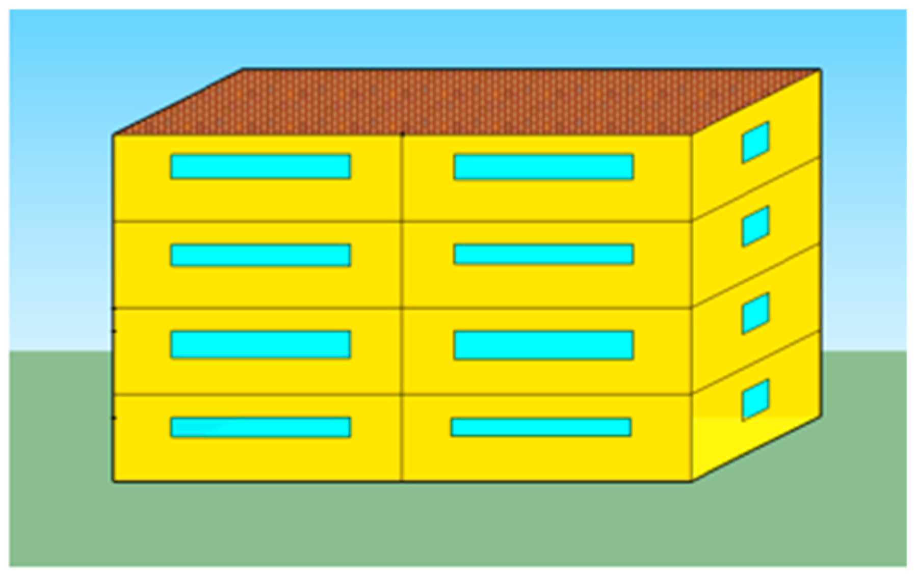
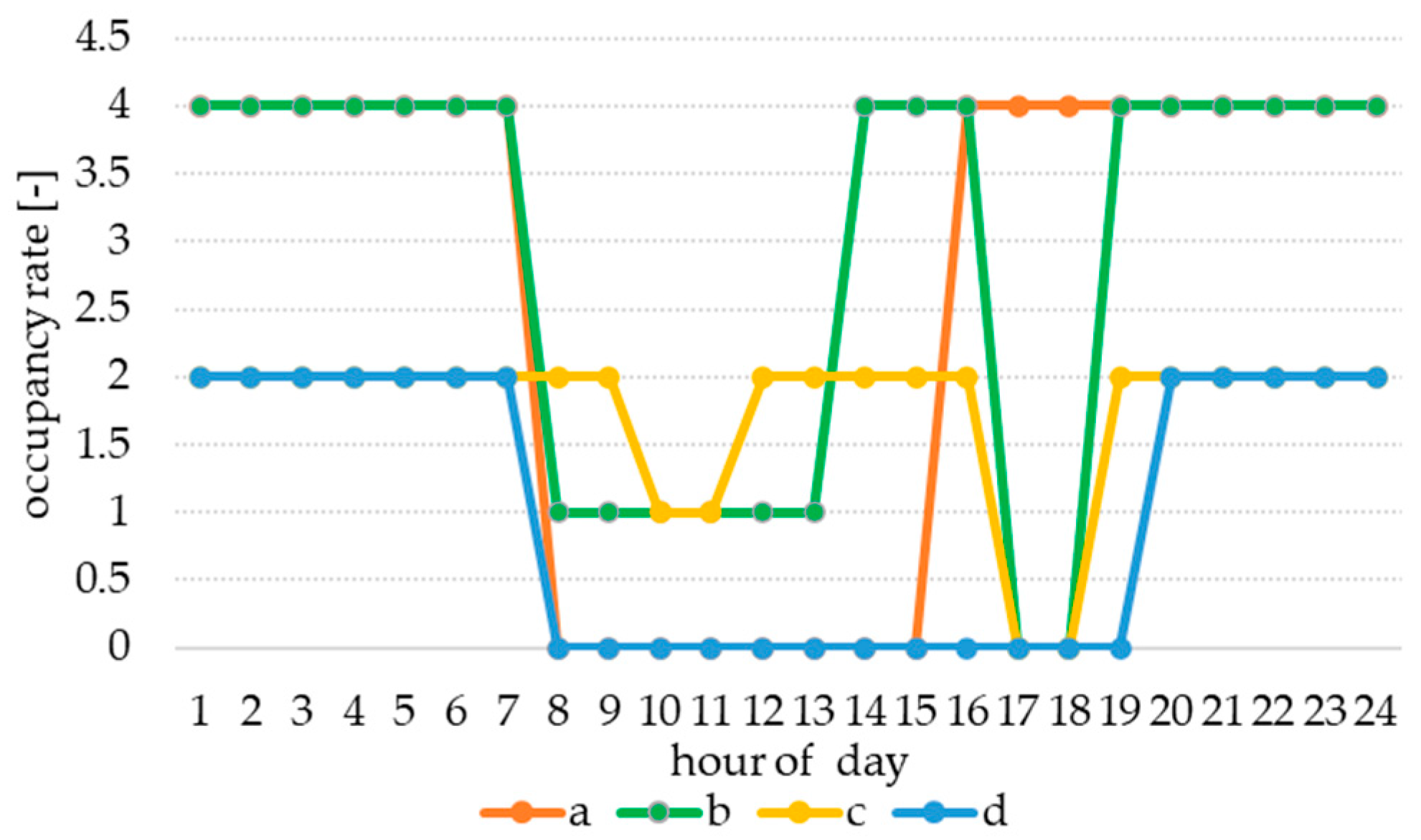
A previous analysis for the building modeling was performed based on a field investigation to define both for the envelope characteristics and users/consumers typologies. The definition and modeling of the building are set up using a tool of TRNSYS software (TRNBUILD). Each building of the district, which is an ensemble of social housing, consists of four floors and eight apartments and is in a residential zone. In the SKETCHUP environment [79], the rendering of the building is represented in Figure 1. Each building consists of four floors with eight thermal zones of 198 m2 and two apartments for each thermal zone; such a configuration was implemented by considering, on one hand, a plausible reproducibility of the considered context and, on the other hand, the computational burden of such a complex layout. The building model reproduces the typical council housing of 1960s. The stratigraphy respects the Italian building regulations for its specific age of construction [80]. All 90 buildings of the district led to a total of 1440 apartments and 1980 habitants, covering ~6% of the Monterusciello population. The opaque and transparent building envelope characteristics and the geometrical parameters for each building are reported in Table 2. The transmittance of windows is referred to a single glass component with aluminum frame. Space heating and cooling loads were evaluated considering an occupancy schedule, represented in Figure 2, based on four different cases (a, b, c, and d):
- case a: two working adults and two children,
- case b: two adults, a child, and an elderly person,
- case c: two elderly habitants, and
- case d: two working adults.
Each one of these schedules refers to two apartments of each considered building.
For the domestic hot water, load is defined as a normalized hourly profile for different months of the year [81] and a daily volume consumption of 50 L per district resident [79].
According to Italian normative [82], the heating period for Naples in climate zone C goes from 15 November to 31 March. While the cooling period is from 1 June to 30 September. The maximum number of heating and cooling systems operating hours is established to 10 h per day.
All the electric energy produced by the plant is sold to the power grid excluding the part needed for auxiliaries of the thermal district network.
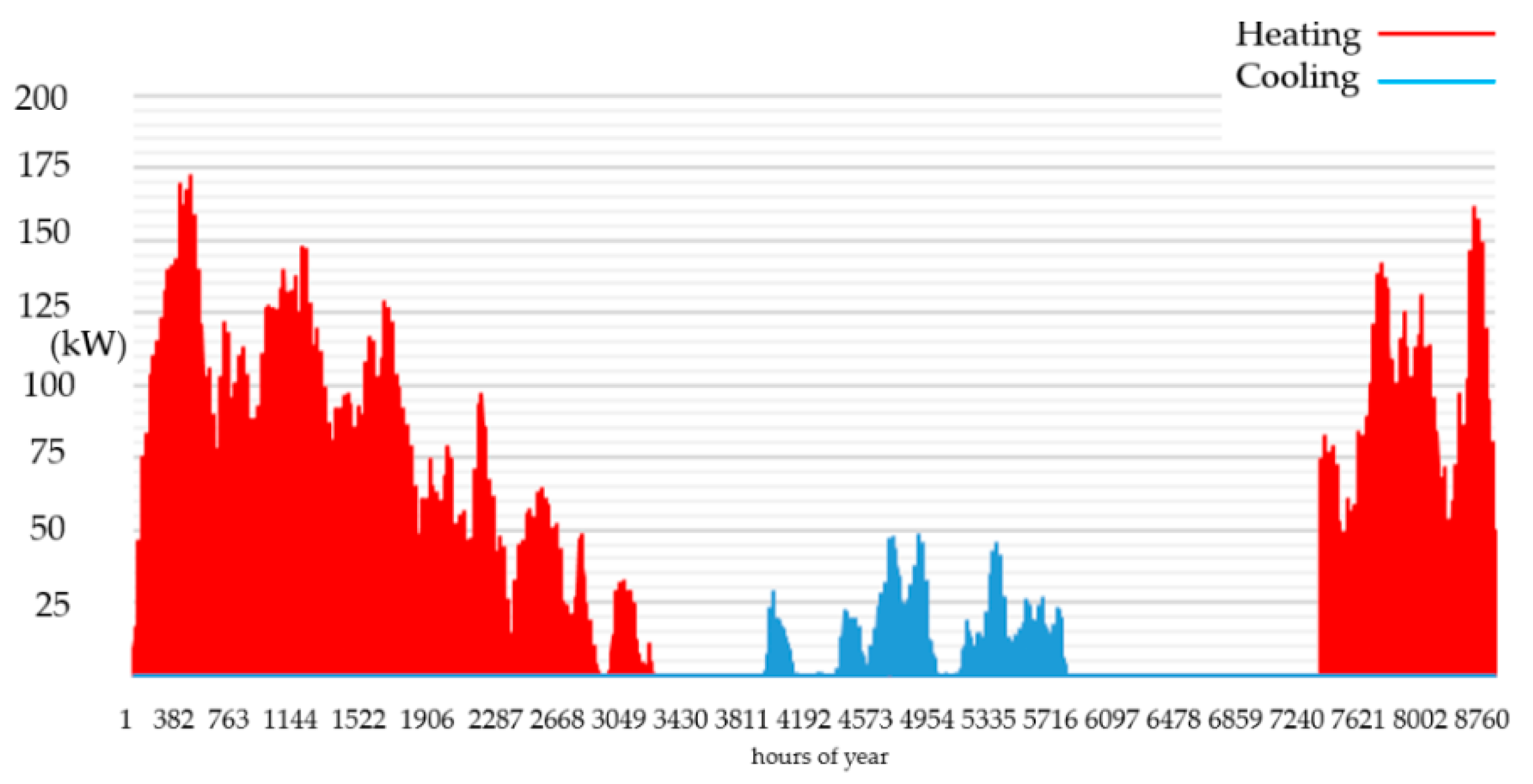
While during the winter period the heating load depends on the desired comfort condition (indoor temperature at 20 °C) required in the whole apartment, during the summer season the energy delivered by cooling network depends by activation of terminal cooling units that commonly serve only the rooms of the apartment effectively occupied. The yearly trends of heating and cooling load for the whole building are presented in Figure 3. The 1-year simulation was based on the weather file available in Trnsys library, which refers to [83].
The buildings of the Monterusciello District area, modeled through TRNBUILD tools and based on the previous information, are connected by means of two energy networks: DHCN and DHWN.
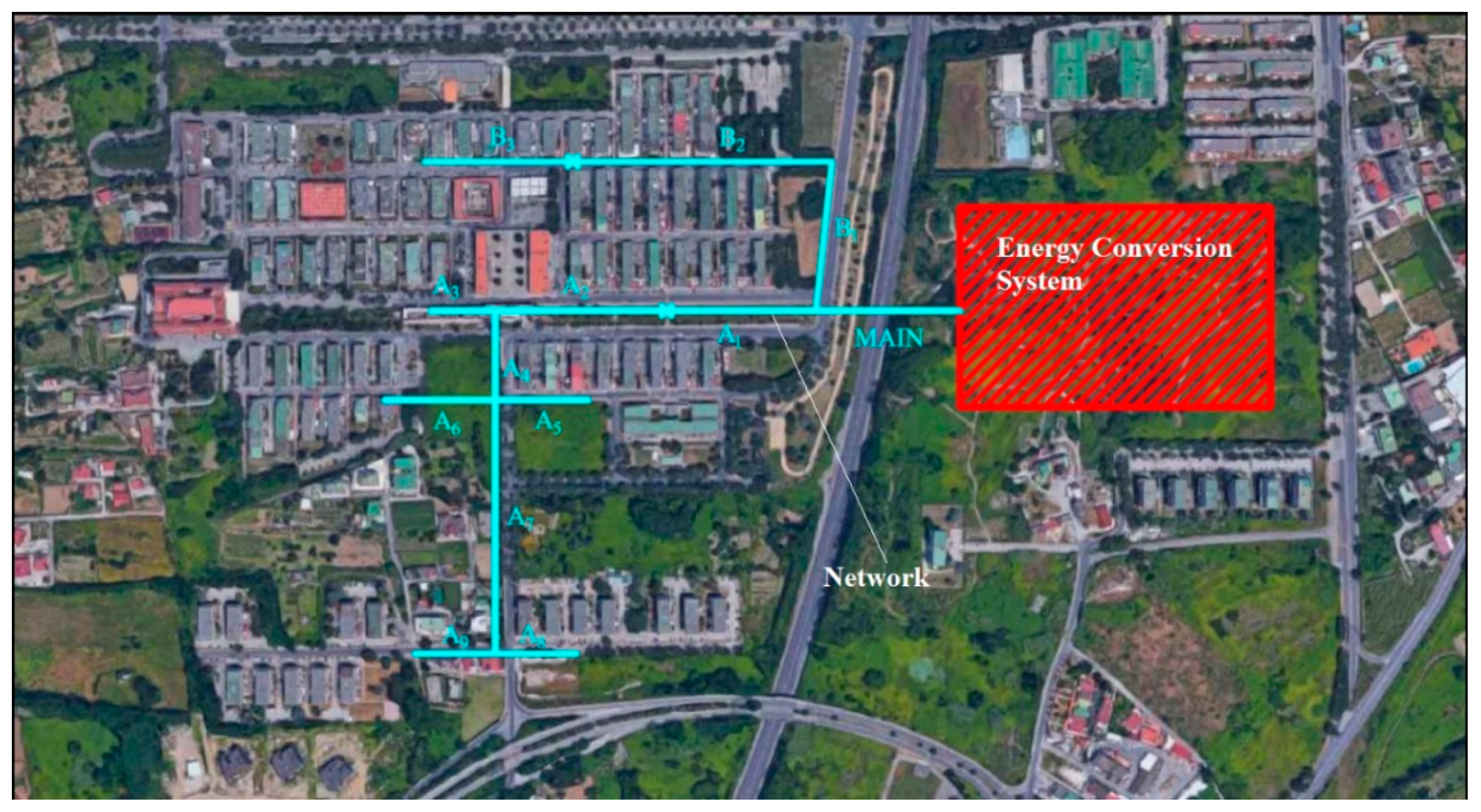
The district area is divided by considering the constraints of the DHCN and DHWN network installation. Figure 4 reports the pipelines segments (in light blue color) running along the main roads, the spatial distribution of the buildings and a viable energy conversion system plant location (in red color). The pipelines segment are labeled as “A” or “B”, referring to different blocks of the district or “MAIN”. The lengths of the pipeline are consequently calculated by considering the real building location and the plausible location of the plant. The diameters sizing takes into account the thermal demand distribution and a fluid velocity of 2.0 m/s is considered. The DHWN sizing was performed similarly to the DHCN one. The geometric features of piping are listed in Table A1 in Appendix. The DHCN considers a time operation of ten hours (from 10 a.m. to 8 p.m.). A parametrical analysis was also conducted to consider the cases in which DHCN is turned off 2 and 4 h later than the base case (10 p.m. and 12 p.m.). The DHW is guaranteed for all 24 h. The set point of DHW temperature is ensured by the biomass boiler. The overall head and thermal losses of the distribution networks takes into account the ones related to the DHCN and the one related to the DHWN.
4. System Configuration and Layout
The simplified system layout is shown in Figure 5, where the main components are presented but the DHCN and the DHWN are omitted. For simplicity of the scheme, only one production well is represented, even if such an analysis two production wells are supposed to be exploited.
First, geofluid powers an ORC module through a heat exchanger (GHE1) heating the hot water (HWORC); the HWORC heats the ORC working fluid in the evaporator.
The ORC is calibrated to ensure a constant power production; it is condensed with cooling water (CW), which is cooled through the cooling tower (CTORC) and whose mass flow rate is adjusted using a variable speed pump to keep the temperature difference at the condenser constant. The ORC module is intended to operate under steady-state conditions with stable evaporation and condensation pressures. This condition at the evaporator is guaranteed by fixed temperature and flow rate of geothermal brine. While to assure the stationary condition at the condenser a variable cooling water flow rate from the water supply net is considered.
A little part of the electricity available from the ORC plant is used to cover the network auxiliaries (pumps, etc.), while the most is sold to the national grid. After delivering thermal energy at ORC evaporator the geothermal fluid is used to provide space heating, cooling, and DHW by means of DHCN and DHWN. A brief description of the system operation and the control strategy is presented herein following a previous study [78].
The Hot Water (HW, red line in the layout) feeding tanks (TK1 and TK3) are produced through the GHE2 heat exchanger. One part of HW is stored in a tank (TK1) to recover thermal energy for space heating and cooling. Through a control strategy, HW is alternatively sent to storage tank TK3, and it is used to store and heat the DHW. Then, a dedicated subsystem is used to ensure a constant temperature.
GHE2 is designed to provide a suitable HW mass flow rate basing on the temperature approach. If the temperature of the HW is higher than that of the geothermal source entering GHE2, the thermostatic valve (through D1/M1) diverts the HW bypassing GHE2, to prevent heat dissipation.
Diverter D2 diverts the HW flow to keep TK1 and TK3 thermally loaded, giving priority to TK1. Different opportune set temperatures on the top of the tanks are provided for both the heating and cooling operation modes. A thermostatic valve (through D3/M3) ensures a constant temperature (45 °C) of the DHW for the networks.
A thermostatic valve (through D4/M4) ensures a constant temperature of the HWDHCN for the DHCN, which is sent directly to the network during the heating operation while it is sent to the adsorption chiller (ADS) during the cooling operation. The HW temperature is set to 50.0 °C during the heating operation and 100 °C during the cooling operation for feeding the ADS. If the set point temperatures cannot be ensured, the biomass boiler (BB) fed with wood chip, is activated until the indicated temperature is reached and until the thermal storage TK1 is thermally loaded. Similarly, if the DHWN set point temperature cannot be ensured, the DHW flow is diverted to the biomass boiler trough thermostatic valve D7/M7.
During the cooling operation, the ADS is activated (by cooling tower, CTADS), and the chilled water (ChWADS) produced is sent to storage tank TK2, where the water ChWDHCN is stored at 10.0 °C and is sent to the DCHN.
To fed DHCN and DHWN the GHE2 is designed to provide a suitable mass flow rate of HW in a temperature range of 40 ÷ 75 °C.
The modeling of the plant has considered an ad hoc defined flow rate for geothermal fluid and a recommended minimum rejection temperature of 70.0 °C as the literature suggestions [84,85]. This value represents a good compromise for avoiding excessive depletion of the geothermal source and moderately mitigating problems involving scaling at the heat exchangers and the mechanical apparatus of the rejection process. Once the geothermal source is set, according to the mass flow rate and temperature range, the available thermal energy is calculated, and the entire system is calibrated accordingly. The ORC is calibrated to ensure constant power production. It is intended to operate under steady-state conditions of working fluid (R245fa); the evaporation and condensation pressures are stable.
5. Models
The development of the whole simulation model has been carried out in three steps, namely, the development of the ORC module in AspenPlus environment, the heat exchanger in AspenEDR environment, and the dynamic simulation model in TRNSYS environment. The TRNSYS library does not include the ORC module; the ORC was implemented in AspenPlus software and simulated by varying the inlet temperature of the source; there were obtained working maps reporting the main output parameters as a function of the inlet temperature of the thermal source, given a constant mass flow rate.
These functions have been implemented in TRNSYS environment adding a user-defined component. The entire dynamic simulation model also includes the ORC heat exchangers modules (evaporator and condenser) and geothermal heat exchangers (GHE1 and GHE2) designed, as previously defined in the introduction section, in the AspenPlus and AspenEDR environments, respectively.
All the heat exchangers of the plant have been developed and designed in AspenEDR environment.
After this, the geometry and suitable heat transfer coefficient correlations have been implemented in TRNSYS software to create a user-defined component: this approach is more rigorous with respect to using the built-in ones since it takes into account the real instant operation of the heat exchanger in terms of overall heat transfer coefficient and efficiency. In the Table A2 in Appendix A all the input parameters of the dynamic model are listed for ORC, working fluid, and heat exchangers. In particular, the heat exchanger GHE1 and GHE2 are simulated considering shell and tube heat exchanger model in titanium material. The resulted characteristics of GHE1 and GHE2 show an external diameter of tubes of 19.05 mm, thickness of tube of 1.2 mm, pitch of 23.8 mm. For the ORC module, the isentropic efficiencies are fixed: 70% and 85% for the pump and turbine, respectively. The ORC pinch point temperature differences are 7 and 5 °C respectively at the evaporator and the condenser. The working fluid used for the ORC plant is the R245fa. The evaporator and condenser for ORC module are two AISI306 shell and tube heat exchangers. The output parameters of the heat-exchanger design and the ORC module obtained as results are presented in Table A3 and Table A4, respectively. In the ORC evaporator (not showed in the layout figure), the inlet and outlet temperatures of R245fa are, respectively, 51.08 and 120.1 °C at 19.35 bar, while at the condenser, they are 66.05°C for the inlet and 50 °C in the outlet section at 3.43 bar. The thermal power exchanged in the evaporator and condenser is 4698 and 3835 kW, respectively.
The nomenclature used to define each parameter in Table A2, Table A3 and Table A4 is referred to system layout scheme represented in Figure 5.
The ORC is calibrated considering a nominal power production of 500 kWel. All the heat exchangers are simulated by calculating the outlet streams’ conditions using the heat and mass balances and the surface area. The inlet and the outlet temperatures of the condensation process are fixed. The mass flow rate is determined accordingly.
Once the cycle is completely defined and simulated in the AspenONE environment, the evaporator and the condenser are designed in AspenEDR.
Both the geothermal heat exchangers (GHE1 and GHE2) are designed by considering plausible values from an ORC market survey of the cold-side mass flow rate for feeding the ORC module, a plausible value of the cold-side temperature difference, and a hot inlet–cold outlet temperature approach. The correlations adopted for the overall heat-transfer coefficient to define heat exchangers parameters are based on the fully developed laminar flow inside the duct with an isothermal wall [86] and the fully developed turbulent flow inside the duct with an isothermal wall [87].
The calibration of the overall system is based on a preventive dynamic simulation of the building equipped with a plausible number of fan coils per apartment, which are also implemented in the TRNSYS environment. Then, according to the simulation results, the heat-exchanger geometry is developed in the TRNSYS environment (with the creation of user-defined components using macros and Calculator blocks) to dynamically simulate the real heat-transfer performance with regard to the instant value of the overall heat-transfer coefficient, efficiency, and number thermal Unit (NTU).
The simulation model of the building is linked to the simulation model of the fan coil in the same TRNSYS environment. The calibration of the fan-coil simulation model is based on a market survey.
The seasonal data about fan coil are listed in the Table 3, such as the nominal power of fan coil (Pnom,fc), flow rate water and air of fan coil (mfc,w, mfc,a), the comfort temperature set (Tset,amb), and the ratio between sensible and total thermal power (Pth,sens/Pth,TOT).
This approach allows us to determine the effective thermal and cooling loads under dynamic operating conditions and then take into account variable weather conditions, the thermal inertia of the building envelope, and the variability of the space occupation.
Once the time-dependent thermal and cooling loads are extrapolated and the maximum thermal energy available from the geothermal source is considered, it is possible to determine the maximum number of apartments served by the system.
Finally, the variable parameters are calibrated in the TRNSYS environment such as mass flow rates, set point temperatures, and characteristics of components under nominal conditions.
The system plant simulation model is linked to the DHCN one, which takes into account the heat losses occurring in the network piping. In turn, the DHCN simulation model is linked to the thermal and cooling loads, allowing the return water conditions to be determined.
6. Methodologies
The system described in the previous sections has been analyzed from an economic an environmental point of view according to the following methodology.
As regards to economic analysis, the total plant investment cost, ZTOT, is given by the sum of the costs of all the modules composing the plant, the cost of the distribution networks, and the BOP (Balance of the Plant) cost ZBOP, to take into account all the auxiliary systems and supporting components of the plant. Table 4 reports the parameters used in the economic analysis, as well as the main parameters of the reference scenarios for each energy vector and emission factor. The performances of the renewable ORC coupled with DHCN system are evaluated by assessing the energetic and economic savings, and by comparing the proposed system (PS) with the reference one (RS). In particular, in case of the reference scenario
- a reversible electric-driven air-to-water heat pump for space heating and cooling is supposed to be installed in each building; the coefficient of performance (COP) in heating mode is supposed to be 3.0, while in cooling mode it is supposed to be 2.5 [88];
- a natural gas boiler for DHW production is supposed to be installed in each dwelling; its efficiency is supposed to be 0.85;
- power production is given by the national grid characterized by an overall average efficiency, ηgrid, equal to 46% [89]
The same space heating and cooling terminal units (fan coils) are adopted both in case of PS and RS.
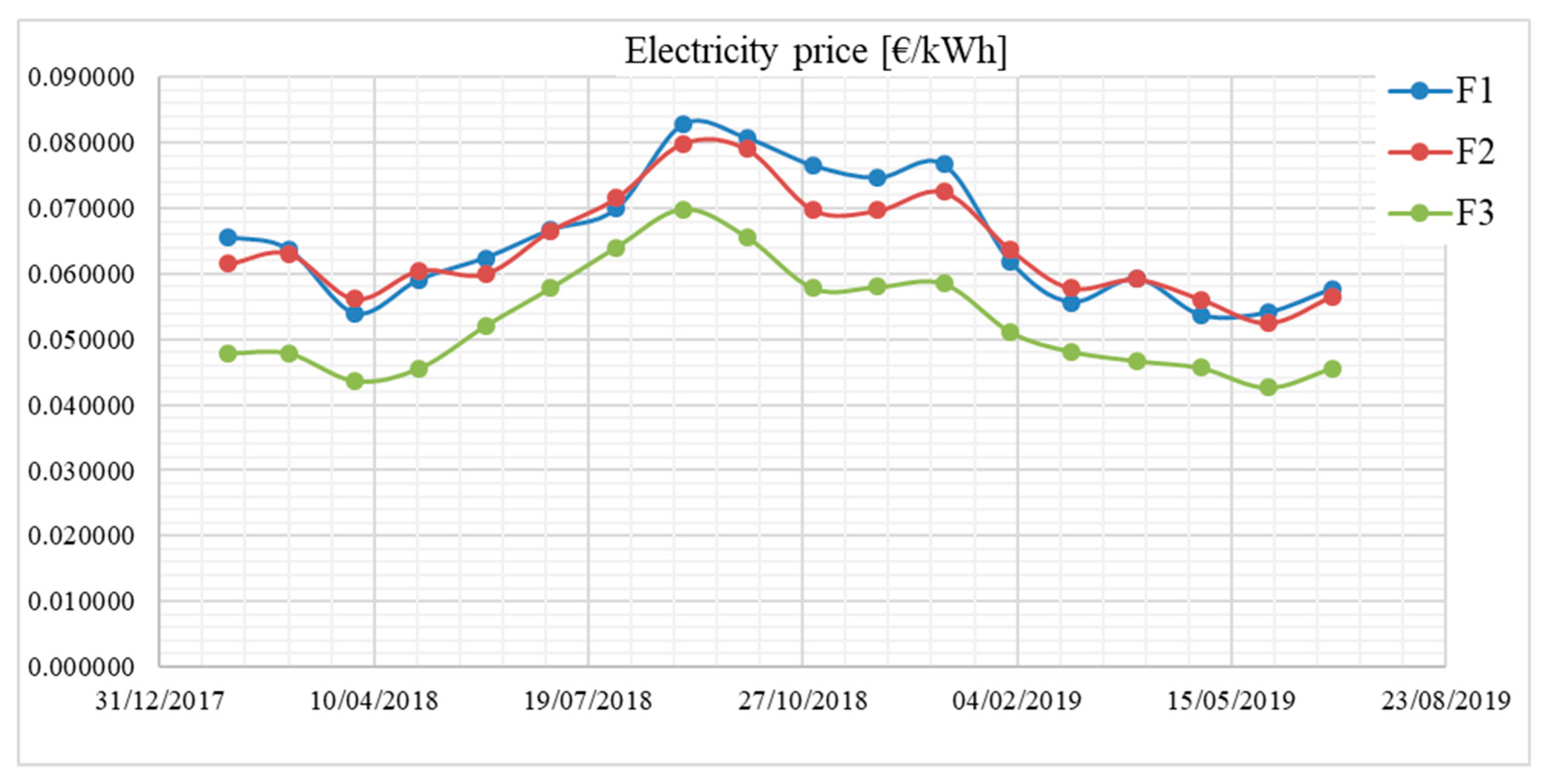
All the electricity prices (for the cases with and without feed-in tariffs) are based on the Italian real market trends from January 2018 to August 2019 [31]. Different prices are provided for the three time-dependent partitions of the Italian market (F1, F2, and F3). The prices of heating and cooling energy are based on market surveys.
The ZBOP is calculated as 3.00% of the overall plant cost. An economic analysis is performed by taking into account two different scenarios for electricity sales: with and without feed-in tariffs provided by the Italian market [31].
In the case of feed-in tariffs, the revenue related to electricity sales Rel,feed-in is defined as follows,
where Eel represents the amount of yearly electricity produced, and cel,feed-in represents the price of electricity under feed-in tariff market conditions. In the case where no feed-in tariffs are provided, a guarantee minimum price tariff system is assumed: regardless of the effective electricity market price, the plant always sells energy above a certain threshold price established by the GSE (Gestore dei Servizi Energetici, i.e., Italian energy services management institution).
Moreover, three selling prices are considered based on the hourly partition of the time-dependent tariff system. Given the uncertainty of the results due to the variability of prices, a plausible range of the revenue (i.e., Rel,min and Rel,max) is calculated according to the minimum and maximum values of the sale price. The minimum and maximum sale price values are established with consideration of the real price trend from January 2018 to August 2019 (reported in Figure A1 in Appendix A).
Then, the minimum and the maximum revenues are calculated as follows,
where the subscript Fi indicates the specific partition of the time-dependent tariff system and the subscript fFi indicates the yearly fraction of the hours belonging to the specific Fi partition.
The revenue related to the selling of thermal energy for space heating Rth is calculated as follows,
where Eth represents the amount of thermal energy provided to the network yearly, and cth represents the price of thermal energy based on an Italian market survey.
Similarly, the revenue related to the selling of cooling energy Rcool is defined as
where Ecool represents the amount of cooling energy provided to the network yearly, and ccool represents the price of cooling energy based on an Italian market survey.
The simple payback (SPB) is defined as follows,
where CFS represents the yearly cash-flow statement, which is defined as
RTOT represents the sum of all the revenues, and CTOT represents the sum of the yearly maintenance cost CO&M and the yearly operational cost COp, which are defined as follows,
where PAUX,TOT represents the total thermal energy provided by the auxiliary boiler, LHVbiom represents the lower heating value of the biomass (wood chips), and cbiom represents the unit cost of the biomass.
Finally, the main economic indicators are calculated to assess the economic profitability of the system, i.e., the discounted payback period (DPB), net present value (NPV), profit index (PI), and internal rate of return (IRR):
where a represents the discount rate, AF represents the annuity factor, and N represents the service life.
Regarding the environmental analysis, the saved primary energy source (PE) is calculated by considering a specific reference scenario for each produced energy vector (electric energy and thermal energy for air conditioning).
Then, the PE is calculated as follows,
where ηboil,ref. represents the reference value for the efficiency of the traditional natural gas boiler, and COPref,HP represents the reference value for the coefficient of performance (COP) of a traditional chiller.
Finally, the avoided CO2 emissions EMCO2 are calculated as follows,
where EFgrid represents the emission factor related to the national grid and EFnat,gas represents the emission factor of the natural gas.
The implemented economic model calculates the investment and the operating costs of both PS and RS. The cost functions adopted for PS and RS components are taken from scientific and technical literature. The cost of GHE1 and GHE2 are obtained by previous literature studies as a function of the heat exchanger area [51]. The tank cost is a function of occupied volume [90]. The cost of line networks for DHCN and DHWN is the functions of diameters and length of pipes [91]. The cost of pumping depends on flow rates which cross the pumps [92].
The study realizes a parametric analysis with different depths of the geothermal well. The depth of the geothermal well affects both the operation of the system plant and economic performance. The aim of the analysis is the prefeasibility study by considering the uncertainty related to the depth where the geothermal source is available and assessing a range for each main performance indicator where the system can be considered feasible and profitable.
A second parametric analysis is performed with different operation times of the DHCN, without changing the operation time of the DHWN; this ensured a constant temperature of 45 °C.
When the DHCN operation time is reduced, a larger amount of electric energy is available, because all the auxiliaries of the DHCN subsystem are off. Consequently, higher revenue related to electricity production is expected.
Additionally, the DHWN subsystem is forced to use the auxiliary biomass boiler to ensure the appropriate temperature of the DHWN; thus, a higher operational cost related to boiler fuel (wood chip) is expected.
The objective is to evaluate the effects of the production strategy on profitability and to determine the optimum operation point.
7. Results
7.1. Thermodynamic Analysis
First, the daily results are presented and discussed through two days representative of the system functioning for each operation mode: one for heating (winter day) and one for cooling (summer day).
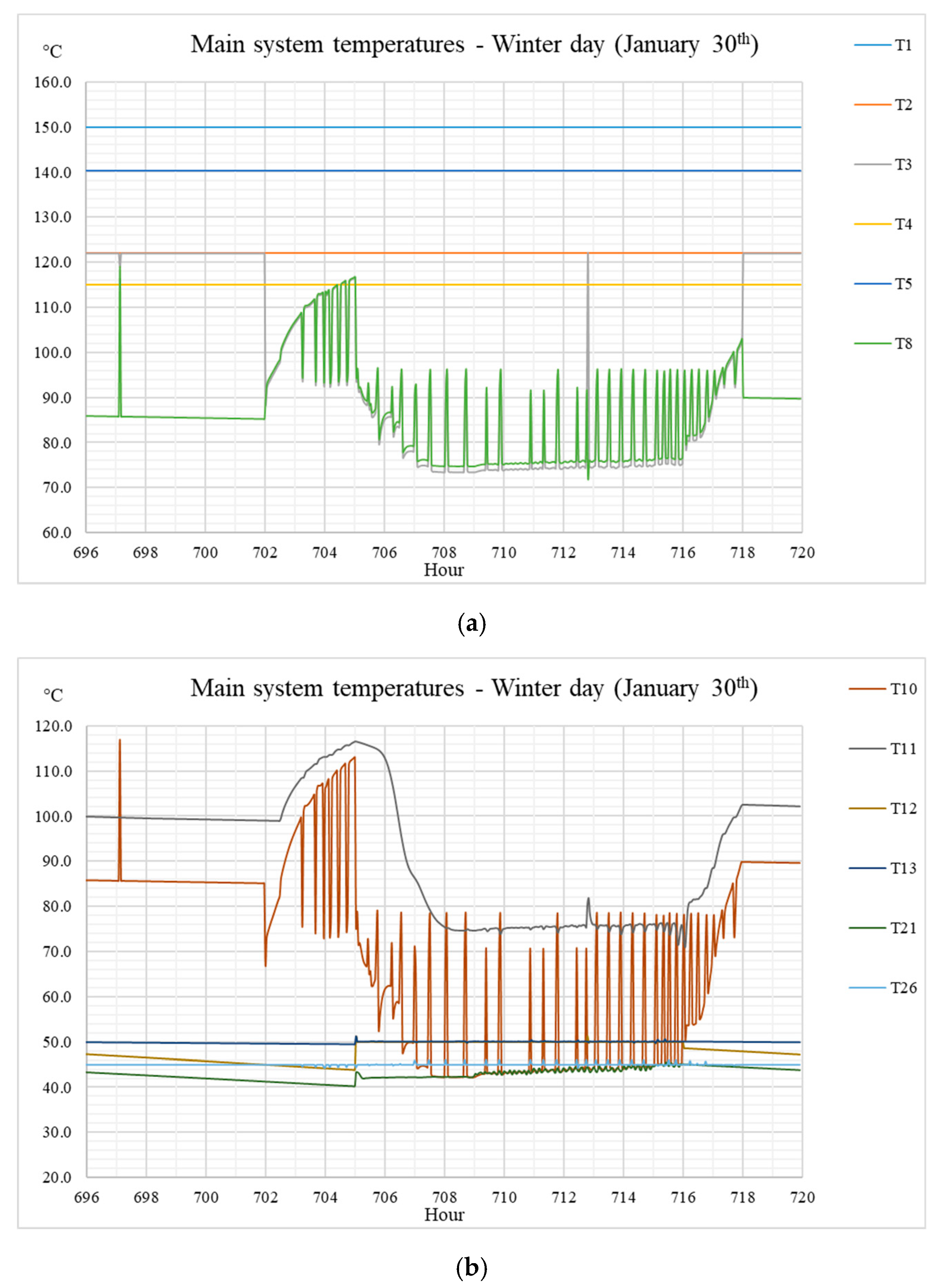
Figure 6 and Figure 7 show the main system outputs, respectively, for the winter day where the nomenclature and numeration refer to Figure 5.
Figure 6 presents the temperatures of the geothermal system for the winter day. T1 and T2 are not reported on the figure. T1 is constant at 150 °C, according to the input parameters, and T2 is constant at 122 °C due to the steady working conditions of the ORC module. T3 varies depending on the time operation of the DHCN and the operation of TK1.
When the DHCN is off, T3 coincides with T2, whereas it continuously varies depending on the inlet condition of the cool side at GHE2, i.e., T10.
T3 never decreases to 70.0 °C, due to the calibration of the overall system and the control strategy.
T10 and T8 exhibit the trends of TK1 to and from GHE2, respectively; T11 and T21 represent the trends of the water temperatures to and from the DHCN, respectively. The system can ensure a constant temperature of 50.0 °C to the DHCN and the set point temperature of the fan coils installed in the apartments taking into account the small heat losses occurring in the piping.
Moreover, the system is capable to give the DHW at a constant temperature value of 45.0 °C, as shown in Figure 6, independently by the load, shown in Figure 7.
From 6:00 to 10:00, the geothermal source is mainly employed to thermally load TK3, which belongs to the DHW subsystem. From 10:00 to 20:00, the source is mainly employed to thermally load TK1, which belongs to the DHCN.
Simultaneously, the geothermal source is constantly employed to feed the ORC module.
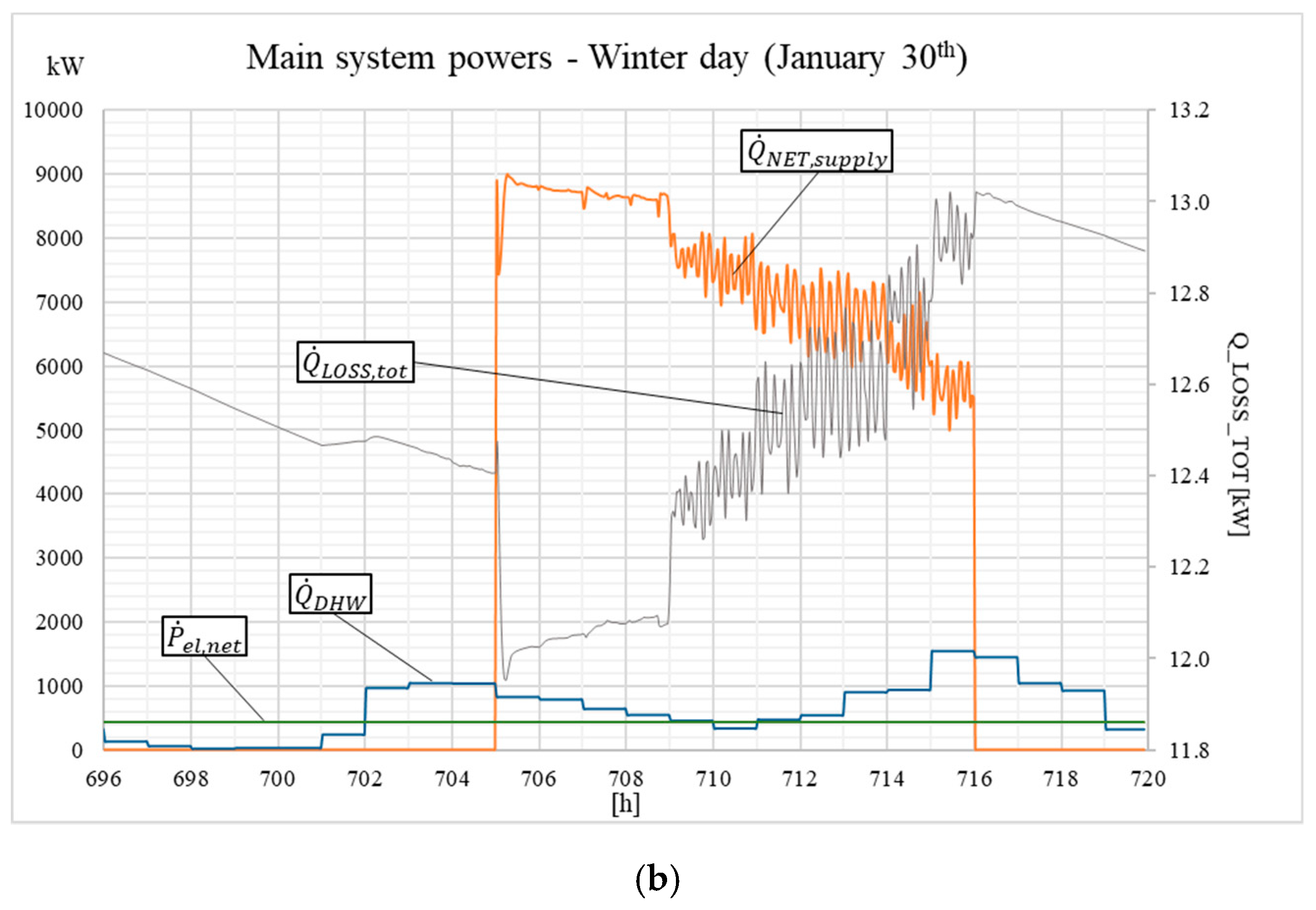
The foregoing is clearly shown in Figure 7, which presents the main system powers.
When the DHCN is off, the amount of achievable thermal power by the geothermal fluid is equivalent approximately to 4.50 MW, whereas it increases to 13.0 MW when the load required by the network is maximized.
The ORC net power production depends on the operation time of the DHCN. When the DHCN is off, the ORC power (approximately 430 kWel) is employed for geothermal fluid pumping and the ORC cooling tower auxiliaries, and the remaining part is sent to the grid.
When the DHCN is on, ORC power is employed to feed all the system auxiliaries (pumps and the overall control and monitoring system). Then, the net power sent to the grid decreases to 380 kWel.
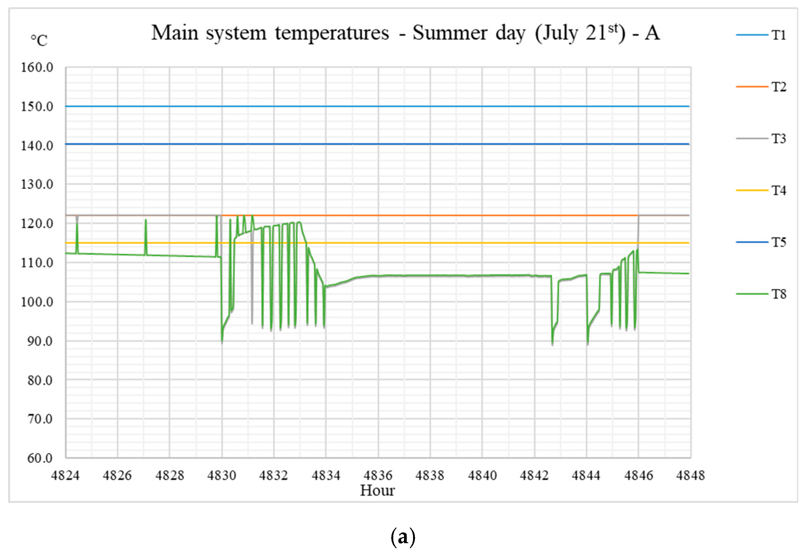
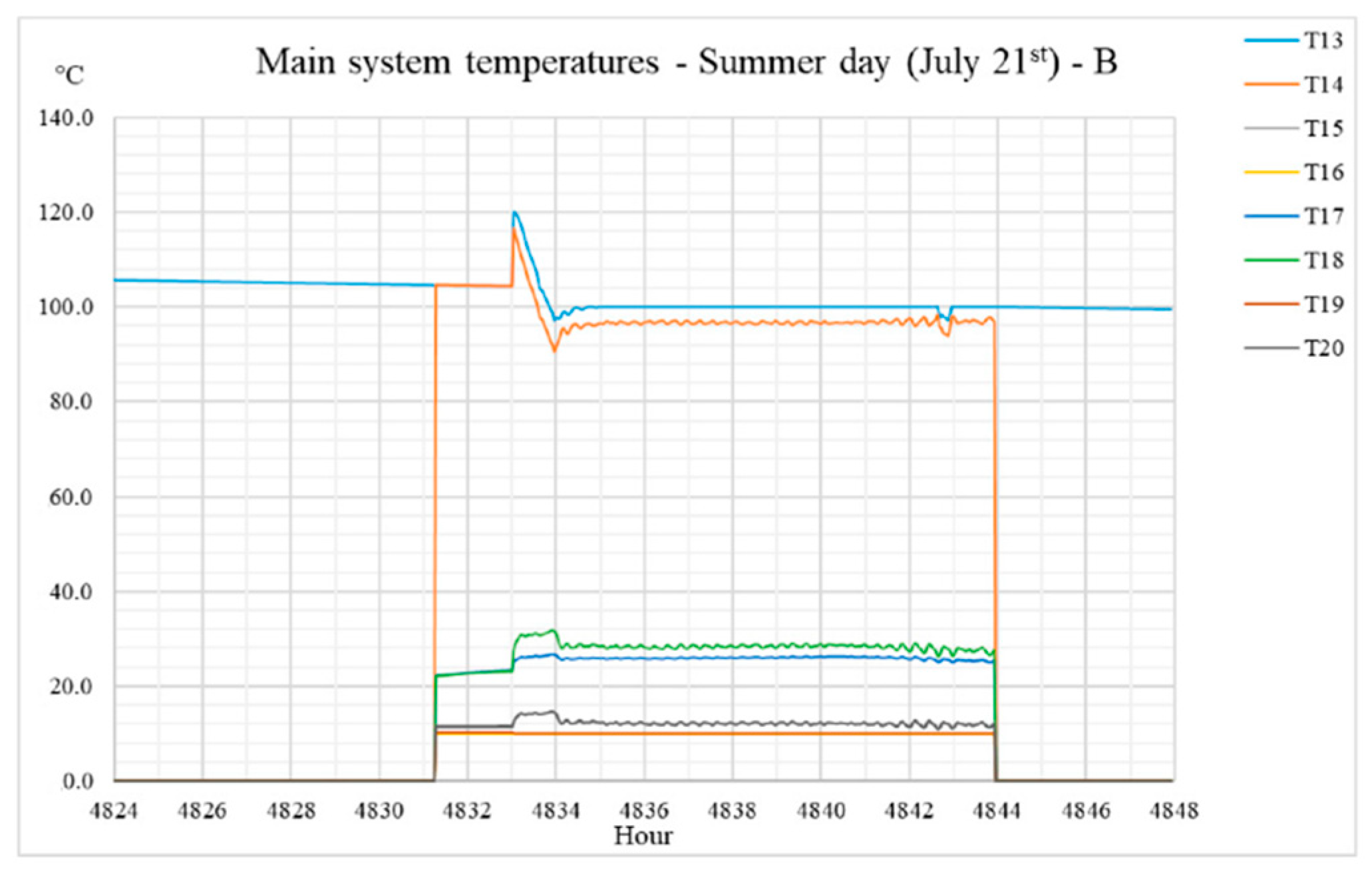
Figure 8 and Figure 9 show the main system temperatures for the characteristic representative summer day, and Figure 10 presents the main system powers.
In particular, Figure 9 indicates the temperature trend of TK3 (T15, T16, T19, T20) and the ADS module (T13, T14, T15, T16, T17, T18). As shown, the feed temperature T13 of the ADS module is constant at 100 °C, except at the initial time, where no cooling load is observed (Figure 10) and the feed water is available at 120 °C. Moreover, the results indicate that the system is perfectly capable of ensuring a constant temperature T19 (10.0 °C) of the cooled water to be sent to the network, which corresponds (taking into account the losses in the network piping) to the set temperature of the fan coil in the cooling mode.
Table 5 presents the main results of the thermodynamic analysis on a monthly and yearly basis.
As shown, the system is perfectly capable of ensuring the temperature levels in each subsystem and it is perfectly capable of covering the total network load required (sum of thermal total power required by DHCN and DHWN) and the losses occurring in the network.
During the heating season, the overall thermal energy provided by the system for district heating, ESUPPLIED,DHCN, is higher than the thermal energy required, Ereq,WINT,DHCN; the difference is caused by the losses occurring at the network piping.
Moreover, the sum given by the thermal energy exiting the TK1, ETK1,out, and the one coming from the auxiliary boiler for the DHCN, EAUX,DHCN, is higher than ESUPPLIED,DHCN: this is due to the thermal losses occurring at the plant piping.
Thermal losses occurring at the thermal storages are given by the difference between the thermal energy entering and exiting the tanks.
What has just been discussed can be referred to the domestic hot water production system.
During the cooling season, the overall cooling energy provided by the system for district cooling, ESUPPLIED,DHCN is higher than the cooling energy required Ereq.SUMM,DHCN; even in this case the difference is caused by the losses occurring at the network piping.
Similarly to the heating season, during the cooling season the cooling energy exiting the TK2 ETK2,out is higher than the supplied one ESUPPLIED,DHCN because of the losses occurring at the system plant.
The gross amount of electricity produced, Pel,ORC, remains constant throughout the year, and Pel,net, which represents the amount of electricity produced and sold to the grid, is lower during the cooling operation than during the heating operation. This is because the entire ADS subsystem, which is off during the heating operation, must be powered.
The constant average first-law efficiency of the ORC is 10.6%, owing to the steady working condition of the module.
The ADS, whose COP is 0.700 under nominal conditions (temperature of the feed hot water equal to 100 °C, the temperature of chilled water equal to 7 °C, and temperature of the cooling water equal to 22 °C), operates during the year with an average COP of 0.660: this is due to fluctuations in operating conditions (in terms of the feed water temperature, cooling water temperature, load), which move the module from the optimum point of operation.
7.2. Environmental and Economic Data Analysis
In this section, the main results of the economic and environmental analyses are presented and briefly discussed. The costs of the components are presented in Table 6, along with the cost function adopted. The total investment cost takes into account three different values of the depth of the geothermal well: the base case at 1500 m and the case of higher depth at 2000 and 2500 m by considering two production and one reinjection wells. Globally, the total investment cost (ZTOT) ranges between 7.84 and 8.21 M€.
Table 7 presents the detailed yearly economic analysis results for each well depth and the different scenarios of the electricity market (with and without feed-in tariffs).
In the case of no feed-in tariffs, the total revenue RTOT ranges from 1.09 to 1.18 M€. With a total operational and maintenance cost CTOT of approximately 0.40 M€, the CFS ranges between 0.69 and 0.78 M€ per year.
All the economic indicators are negatively affected by the low CFS, and the system appears to be unprofitable.
The SPB period exhibits a minimum value of 10.0 years and a maximum value of 11.9 years. These are far higher than the acceptable range of 5.00 to 7.00 years for private investments.
With a discount rate of 5.00%, the DPB period increases (minimum value of 14.3 years and maximum value of 18.5 years).
The NPV exhibits low values ranging between 0.388 and 1.88 M€, corresponding to a PI ranging between 4.73% and 24.0%. Acceptable values of the PI are between 60.0% and 70.0%.
Finally, the IRR exhibits low values between 5.51% and 7.64%
The economic profitability is improved in the case of the feed-in tariffs for electricity selling.
In fact, given the constant revenues related to the thermal and cooling energy for air conditioning, Rth, and Rcool, as well as the constant operational and maintenance costs CTOT, in correspondence of CFS value of 1.12 M€ the higher revenue related to power production Rel are equal to 0.631 M€.
Consequently, acceptable values of the SPB and DPB are obtained.
The SPB period ranges between 7.00 and 7.33 years, and the DPB period ranges between 8.84 and 9.36 years.
The NPV is increased to values between 5.74 and 6.11 M€, corresponding to PIs of 69.9% and 77.9%, respectively.
Finally, the IRR ranges between 12.2% and 13.0%.
Globally, as shown in Table 8, such a renewable system allows avoiding the employment of 27.2 GWh of primary energy and (depending on the reference scenario adopted for the energy and material outputs) avoiding 5.49 × 10³ tons of CO2 emissions.
The main results of the thermodynamic and economic analyses performed by varying the operation time of the DHCN are presented from Table A5, Table A6, Table A7, Table A8 and Table A9 in Appendix A. In detail, the data about electricity production (Rel), the CFS, the SPB, the NPV, and the PIs in the case of feed-in tariffs (green) and the cases of the minimum and maximum selling prices of electricity are reported.
Longer operation time of the DHCN subsystem corresponds to higher economic profitability: all the economic indices are affected by lower DHCN operation time.
In fact, in the case of the longest time of operation, a slightly lower amount of electricity is sold to the grid because the auxiliaries are on, and the revenue related to electricity is lower as well.
On the other hand, a higher amount of thermal energy is available from the geothermal source, then avoiding the use of biomass and reducing the operational cost of the biomass boiler to supply the DHW.
In case of the shortest time of operation, a higher amount of electricity is available (auxiliaries are off) for the selling. At the same time, any load from DHW network is cover by the biomass boiler, and a higher operational cost related to boiler fuel is obtained.
The higher operational cost of the biomass boiler prevails on the higher revenue related to electricity when the time of operation is reduced and the global profitability decreases.
The revenues related to space heating and cooling are constant.
It is worth noticing that, despite the analysis was carried out with the greatest possible precision, the results strictly depend on the specific case study analyzed and on the considered market context; moreover, they are affected by unavoidable uncertainty given by
- -
- weather conditions, which affect the electric and thermal loads, and the ORC operation (including the cooling tower);
- -
- real availability of geothermal source, which can be assessed only after a specific exploration campaign;
- -
- fluctuations of the electricity prices and variation of the feed-in tariffs system; and variations of prices related to district heating and cooling (even though they are characterized by more stability if compared to electricity one).
8. Conclusions
A thermodynamic, economic, and environmental analysis of a renewable polygeneration system connected to a DHCN was performed.
The system is designed for a suburban area of the metropolitan city of Naples (South of Italy) and it is powered by geothermal sources and biomass, producing electricity, thermal energy for space heating and cooling, and DHW production.
The entire dynamic simulation model (which includes an organic Rankine cycle module, an ADS, an auxiliary biomass boiler, geothermal heat exchangers, thermal storage tanks, the DHCN, residential systems of space conditioning including terminals, and a suitable model of the building envelope) was developed and implemented in AspenONE and TRNSYS environments.
The layout and the control strategy were implemented to match the appropriate operating temperature levels for each component and to prevent the temperature of the geothermal fluid reinjected into the wells from decreasing below 70.0 °C.
The overall component calibration and the economic analysis were based on manufacturer data and market surveys.
The economical returns are estimated by considering the electric power sold to the national grid. Differently, the thermal energy for heating and cooling is employed to satisfy the thermal yearly load of the whole district.
An analysis was performed with different depths of geothermal wells where the source is available considering a geothermal temperature gradient of 0.1 °C/m.
An economic analysis was performed for two different electricity purchase scenarios: with and without feed-in tariffs.
The system, whose investment cost ranges between 7.84 and 8.02 M€, is economically feasible only under feed-in tariff conditions.
In fact, without feed-in tariffs, economic indicators suggest that the system is unprofitable: the minimum SPB period is 10.1 years (corresponding to a DPB period of 14.3 years if a discount rate of 5.00% is applied), and the maximum NPV is 1.88 M€ (corresponding to a maximum PI of 24.0%).
Finally, the maximum IRR is 7.64%.
Conversely, if feed-in tariffs are considered, the economic indicators suggest that for the specific case study analyzed, the system is attractive.
The minimum SPB period is 7.00 years, corresponding to a DPB period of 8.84 years.
The maximum NPV is increased to 6.11 M€, corresponding to a PI of 77.9%. The maximum IRR is 13.0%.
The system allows avoiding exploitation of 27.2 GWh of primary energy yearly, corresponding to 5.49 × 10³ tons of CO2 emissions avoided yearly.
The keys to making the small-medium scale systems powered with geothermal sources feasible and attractive are the polygeneration and the load-sharing, which aim at maximizing the source exploitation by diversifying the energy and material vectors produced and by obtaining loads and requests that are distributed over time to the greatest extent possible.
In future studies, different typologies of final users and different energy vectors could be considered using the sources availability 24 h/24 h to feed the plant.
Author Contributions
Conceptualization, F.C., A.M., E.M., C.R. and L.V.; methodology, F.C., A.M., E.M., C.R. and L.V.; software, F.C., A.M. and E.M.; formal analysis, F.C., A.M. and E.M.; investigation, F.C., A.M. and E.M.; resources, C.R. and L.V.; data curation, F.C., A.M. and E.M.; writing—original draft preparation, F.C., A.M. and E.M.; writing—review and editing, F.C., A.M. and E.M.; visualization, F.C., A.M. and E.M.; supervision, C.R. and L.V.; project administration, C.R. and L.V.; funding acquisition, C.R. and L.V.; All authors have read and agreed to the published version of the manuscript.
Funding
This research was funded by the GeoGrid project POR Campania FESR 2014/2020 CUP B43D18000230007.
Acknowledgments
The authors gratefully acknowledge the financial support of provided through the GeoGrid project POR Campania FESR 2014/2020 CUP B43D18000230007. Nicola Massarotti gratefully acknowledges the local program of the University of Napoli “Parthenope” for the support of individual research.
Conflicts of Interest
The authors declare no conflict of interest.
Nomenclature
| A | Area (m2) |
| a | discount rate (-) |
| AF | annuity factor |
| BOP | Balance of the Plant |
| C | Cost (€, k€, M€) |
| c | unit price (€/specific unit of measurement) |
| CFS | cash-flow statement (€, k€, M€) |
| COP | coefficient of performance (-) |
| d | Diameter (mm) |
| DPB | discounted payback (y) |
| E | Energy (kWh, MWh, kJ, MJ) |
| EMCO2 | avoided CO2 emissions (-,%) |
| EF | emission factor (kgCO2/MWhel, tCO2/TJ) |
| H | geothermal well depth (m) |
| L | Length (m) |
| LHV | lower heating value (kJ/kg, kWh/m3, MWh/t) |
| ṁ | mass flow rate (kg/s) |
| N | service life (y) |
| NPV | net present value (M€) |
| IRR | internal rate of return (-) |
| Ṗ | Power (kW) |
| p | pressure (bar) |
| PE | primary energy (MWh) |
| PI | profit index (-) |
| E | thermal energy (kWh, MWh, kJ, MJ) |
| R | Revenue (€, k€, M€) |
| SPB | simple payback (y) |
| T | Temperature (°C) |
| t | ton |
| U | Transmittance (W/(m2K)) |
| V | Volume (m3) |
| Z | investment cost (€, k€, M€) |
| Superscripts and Acronyms | |
| a | air |
| amb | ambient |
| ADS | adsorption chiller |
| AUX | auxiliary |
| AVG | average |
| biom | biomass |
| boil | boiler |
| BB | biomass boiler |
| BOP | Balance Of Plant |
| chil | electric chillers |
| CT | cooling tower |
| ChW | chilled water |
| CW | cooling water |
| cool | cooling |
| CO2 | carbon dioxide |
| D | diverter |
| DHCN | district heating and cooling network |
| DHW | domestic hot water |
| DHWN | domestic hot water network |
| el | electric |
| F | timeslot of electricity market |
| fi | yearly fraction of -ith timeslot of electricity market |
| fc | fan coil |
| geo | geothermic/geothermal |
| GF | geothermal fluid |
| GHE | geothermal heat exchanger |
| grid | power plant grid |
| h | hour |
| heat | heating |
| hot | hot |
| HP | traditional heat pump |
| HW | hot water |
| in | inlet |
| is | isentropic |
| LMTD | logarithm mean temperature difference (K) |
| LOSS | losses |
| max | maximum |
| min | minimum |
| M | mixer |
| nat, gas | natural gas |
| net | net |
| nom | nominal |
| NTU | number thermal unit |
| O & M | operation and maintenance |
| Op | operative |
| out | outlet |
| ORC | organic Rankine cycle |
| P | pump |
| piping | piping |
| PS | proposed system |
| ref | reference scenario |
| req | required |
| RES | renewable energy sources |
| RS | reference system |
| s | shell |
| sens | sensible |
| set | setpoint |
| SUPPLY | supplied |
| SUMM | summer |
| th | thermal |
| TOT | total |
| TK | thermal storage tank |
| w | water |
| wf | working fluid |
| WINT | winter |
| Greek Letters | |
| ε | heat-exchanger efficiency (-) |
| η | isentropic efficiency/first-law efficiency (-) |
Appendix A
Appendix A.1. Input Parameters

Table A1.
Lengths and diameters of the main line and of the pipes of the subdistrict.
| Network Piping | ||
|---|---|---|
| Segment | Length (m) | Diameter (mm) |
| MAIN | 90 | 300 |
| A1 | 80 | 250 |
| A2 | 80 | 250 |
| A3 | 70 | 175 |
| A4 | 80 | 250 |
| A5 | 50 | 200 |
| A6 | 80 | 200 |
| A7 | 70 | 200 |
| A8 | 50 | 175 |
| A9 | 70 | 175 |
| B1 | 100 | 250 |
| B2 | 100 | 250 |
| B3 | 60 | 200 |
Table A2.
Main thermodynamic and design input parameters.
| Parameter | Value |
|---|---|
| mgeo (kg/s) | 40.00 |
| mHW_ORC (kg/s) | 44.15 |
| mHW (kg/s) | 268.3 |
| mChW_ADS (kg/s) | 268.3 |
| mHW_DHCN (kg/s) | 268.3 |
| p1 (bar) | 8.000 |
| T1 (°C) | 150.0 |
| T2 (°C) | 122.0 |
| T3 (°C) | >70.00 |
| T4 (°C) * | 115 |
| T5 (°C) * | 140 |
| T6 (°C) * | 20.0 |
| T7 (°C) * | 45.00 |
| T10 (°C) * | 40.0 |
| T8 (°C) * | 78.0 |
| Ṗel,ORC (kW) ** | 500.0 |
| Ṗel,2 (kW) ** | 13.4 |
| Ṗel,3 (kW) ** | 13.40 |
| Ṗel,4 (kW) ** | 13.4 |
| Ṗel,5 (kW) ** | 13.4 |
| COPADS(-) * | 0.70 |
| Pth,BB (kW) ** | 2000.0 |
| Pnom.ADS (kW) ** | 7000.00 |
| VTK1 (m3) | 160.0 |
| VTK2 (m3) | 160.0 |
| VTK3 (m3) | 60.0 |
* Under nominal conditions. ** Rated power.
Table A3.
Geothermal heat exchanger output parameters.
| Parameter | Value |
|---|---|
| GHE1 | |
| AGHE1 (m2) | 175.9 |
| Tube number (plain) (-) | 248.0 |
| LGHE1 (m) | 6.0 |
| Number of tube passes (-) | 1 |
| Number of tube passes (-) | 1 |
| ds,GHE1 (mm) | 457.2 |
| Number of segmental baffles (-) | 10 |
| Ṗth,GHE1 (kW) * | 4698 |
| εGHE1 (-) * | 0.7851 |
| TLMTD (°C) * | 8.53 |
| FGHE1 (-) | 1.02 |
| GHE2 | |
| AGHE2 (m2) | 106.6 |
| Tube number (plain) (-) | 296.0 |
| LGHE2 (m) | 6.096 |
| Number of tube passes (-) | 1.000 |
| Number of tube passes (-) | 1.000 |
| ds,GHE2 (mm) | 498.5 |
| Number of segmental baffles (-) | 10.00 |
| Ṗth,GHE2 (kW) * | 9659 |
| εGHE2 (-) * | 0.6365 |
| TLMTD (°C) * | 36.69 |
* Under nominal conditions.
Table A4.
Main ORC output parameters.
| Parameter | Value |
|---|---|
| Evaporation pressure (bar) | 19.35 |
| Condensation pressure (bar) | 3.432 |
| Evaporation temperature (°C) | 120.1 |
| Condensation temperature (°C) | 50.00 |
| mR245fa (kg/s) | 20.04 |
| Evaporator heat exchanger area (m2) | 207.7 |
| Condenser heat exchanger area (m2) | 214.2 |
Figure A1.
Electricity price from January 2018 to August 2019 for every partition (F1, F2, and F3) of the time-dependent tariff.
Figure A1.
Electricity price from January 2018 to August 2019 for every partition (F1, F2, and F3) of the time-dependent tariff.

Appendix A.2. Cost Functions
In the following are the cost functions used in the economic analysis; it is also indicated the reference the function was taken from.
The cost of the well zwell, which is divided into three different segments, is a function of the diameter and depth of each segment. In this work, two production well and one reinjection well were supposed.
Appendix A.3. Main Results of Thermodynamic Analysis
Table A5.
Main results of the thermodynamic analysis (stop time of the DHCN at 20:00).
| Thermal/Electrical Energy | Jan | Feb | Mar | Apr | May | June | July | Aug | Sept | Oct | Nov | Dec | Year |
|---|---|---|---|---|---|---|---|---|---|---|---|---|---|
| Egeo (MWh) | 6309 | 5726 | 5739 | 3776 | 3884 | 3833 | 4307 | 4195 | 3839 | 3863 | 4710 | 6214 | 56,394 |
| ETK1,in (MWh) | 2486 | 2261 | 1877 | 24 | 16.55 | 95.5 | 490.9 | 362.6 | 117.2 | 13.4 | 990 | 2392 | 11,125 |
| ETK1,out (MWh) | 2475 | 2257 | 1866 | 7.753 | 2.644 | 81.49 | 481.1 | 347.1 | 98.24 | 0.000 | 995 | 2376 | 10,987 |
| ETK2,in (MWh) | 0.000 | 0.000 | 0.000 | 4.159 | 0.9846 | 51.63 | 403.6 | 270.9 | 62.57 | 0.000 | 0.000 | 0.000 | 793.8 |
| ETK2,out (MWh) | 0.000 | 0.000 | 0.000 | 3.746 | 0.1533 | 50.45 | 402.2 | 269.2 | 61.37 | 0.000 | 0.000 | 0.000 | 787.2 |
| Eheat,ADS (MWh) | 0.000 | 0.000 | 0.000 | 6.04 | 1.797 | 81.6 | 600.3 | 408.4 | 97.41 | 0.000 | 0.000 | 0.000 | 1196 |
| Ecool,ADS (MWh) | 0.000 | 0.000 | 0.000 | 4.195 | 1.053 | 51.73 | 403.7 | 271 | 62.65 | 0.000 | 0.000 | 0.000 | 794.3 |
| Ereq,WINT,DHCN (MWh) | 2518 | 2294 | 1860 | 0.000 | 0.000 | 0.000 | 0.000 | 0.000 | 0.000 | 0.000 | 997.7 | 2402 | 10,072 |
| Ereq,SUMM,DHCN (MWh) | 0.000 | 0.000 | 0.000 | 0.000 | 0.000 | 48.8 | 399.8 | 265.5 | 57.58 | 0.000 | 0.000 | 0.000 | 771.6 |
| ESUPPLIED,DHCN (MWh) | 2527 | 2304 | 1871 | 0.000 | 0.000 | 50.36 | 402.2 | 269.2 | 61.29 | 0.000 | 1003 | 2411 | 10,900 |
| ETK3,in (MWh) | 331.8 | 309.8 | 373.7 | 358.7 | 361.1 | 346.5 | 313.2 | 330.1 | 329.2 | 343.1 | 336.1 | 334.2 | 4068 |
| ETK3,out (MWh) | 327.3 | 303.6 | 365.9 | 357.8 | 360.2 | 345.4 | 312.2 | 329.1 | 328.4 | 342.3 | 332.1 | 326.4 | 4031 |
| Ereq,DHW (MWh) | 468.1 | 428.7 | 476.4 | 457.9 | 465.3 | 440.4 | 445.3 | 438.4 | 422.5 | 440 | 433.5 | 458.2 | 5375 |
| ESUPPLIED,DHW (MWh) | 468.4 | 429 | 476.5 | 457.9 | 465.4 | 440.4 | 445.1 | 438.2 | 422.4 | 440.1 | 433.5 | 458.5 | 5376 |
| EAUX,DHCN (MWh) | 56.76 | 49.17 | 8.054 | 0.033 | 0.000 | 1.923 | 120.27 | 65.5 | 2.905 | 0 | 8.823 | 40.42 | 353.9 |
| EAUX,DHW (MWh) | 141.1 | 125.37 | 110.55 | 100.15 | 105.21 | 94.96 | 132.95 | 109.08 | 94.04 | 97.79 | 101.43 | 132.11 | 1344.7 |
| ELOSS,DHCN (MWh) | 7.368 | 7.296 | 8.894 | 0.5708 | 0.3691 | 1.386 | 2.476 | 3.402 | 3.615 | 1.212 | 2.889 | 6.17 | 45.65 |
| ELOSS,DHW (MWh) | 1.252 | 1.249 | 1.42 | 1.31 | 1.197 | 0.9611 | 0.7958 | 0.6574 | 0.5994 | 0.6895 | 0.8208 | 1.053 | 12.01 |
| Eel,ORC (MWh) | 372 | 336 | 372 | 360 | 372 | 360 | 372 | 372 | 360 | 372 | 360 | 372 | 4380 |
| Eel,net (MWh) | 327.4 | 295.9 | 328.8 | 312.3 | 322.8 | 312.1 | 322.1 | 322.1 | 312.3 | 330 | 318.5 | 328.2 | 3832 |
| COPAVG (-) | 0.000 | 0.000 | 0.000 | 0.6944 | 0.5861 | 0.634 | 0.6724 | 0.6634 | 0.6432 | 0.000 | 0.000 | 0.000 | 0.6643 |
| ηORC (%) | 10.64 | 10.64 | 10.64 | 10.64 | 10.64 | 10.64 | 10.64 | 10.64 | 10.64 | 10.64 | 10.64 | 10.64 | 10.64 |
Table A6.
Main results of the thermodynamic analysis (stop time of the DHCN at 22:00).
| Thermal/Electrical Energy | Jan | Feb | Mar | Apr | May | June | July | Aug | Sept | Oct | Nov | Dec | Year |
|---|---|---|---|---|---|---|---|---|---|---|---|---|---|
| Egeo (MWh) | 6309 | 5726 | 5739 | 3776 | 3884 | 3833 | 4307 | 4195 | 3839 | 3863 | 4710 | 6214 | 56,394 |
| ETK1,in (MWh) | 2486 | 2261 | 1877 | 24.00 | 16.55 | 95.50 | 490.9 | 362.6 | 117.2 | 13.40 | 990.0 | 2392 | 11,125 |
| ETK1,out (MWh) | 2475 | 2257 | 1866 | 7.753 | 2.644 | 81.49 | 481.1 | 347.1 | 98.24 | 0.000 | 995 | 2376 | 10,987 |
| ETK2,in (MWh) | 0.000 | 0.000 | 0.000 | 4.159 | 0.9846 | 51.63 | 403.6 | 270.9 | 62.57 | 0.000 | 0.000 | 0.000 | 793.8 |
| ETK2,out (MWh) | 0.000 | 0.000 | 0.000 | 3.746 | 0.1533 | 50.45 | 402.2 | 269.2 | 61.37 | 0.000 | 0.000 | 0.000 | 787.2 |
| Eheat,ADS (MWh) | 0.000 | 0.000 | 0.000 | 6.04 | 1.797 | 81.6 | 600.3 | 408.4 | 97.41 | 0.000 | 0.000 | 0.000 | 1196 |
| Ecool,ADS (MWh) | 0.000 | 0.000 | 0.000 | 4.195 | 1.053 | 51.73 | 403.7 | 271 | 62.65 | 0.000 | 0.000 | 0.000 | 794.3 |
| Ereq,WINT,DHCN (MWh) | 2518 | 2294 | 1860 | 0.000 | 0.000 | 0.000 | 0.000 | 0.000 | 0.000 | 0.000 | 997.7 | 2402 | 10,072 |
| Ereq,SUMM,DHCN (MWh) | 0.000 | 0.000 | 0.000 | 0.000 | 0.000 | 48.8 | 399.8 | 265.5 | 57.58 | 0.000 | 0.000 | 0.000 | 771.6 |
| ESUPPLIED,DHCN (MWh) | 2527 | 2304 | 1871 | 0.000 | 0.000 | 50.36 | 402.2 | 269.2 | 61.29 | 0.000 | 1003 | 2411 | 10,900 |
| ETK3,in (MWh) | 331.8 | 309.8 | 373.7 | 358.7 | 361.1 | 346.5 | 313.2 | 330.1 | 329.2 | 343.1 | 336.1 | 334.2 | 4068 |
| ETK3,out (MWh) | 327.3 | 303.6 | 365.9 | 357.8 | 360.2 | 345.4 | 312.2 | 329.1 | 328.4 | 342.3 | 332.1 | 326.4 | 4031 |
| Ereq,DHW (MWh) | 468.1 | 428.7 | 476.4 | 457.9 | 465.3 | 440.4 | 445.3 | 438.4 | 422.5 | 440 | 433.5 | 458.2 | 5375 |
| ESUPPLIED,DHW (MWh) | 469.4 | 429.9 | 477.8 | 459.2 | 466.5 | 441.4 | 446.1 | 439.1 | 423.1 | 440.7 | 434.3 | 459.3 | 5387 |
| EAUX,DHCN (MWh) | 50.49 | 44.19 | 6.964 | 0.000 | 0.000 | 1.612 | 118.73 | 65.72 | 2.466 | 0.000 | 8.032 | 34.43 | 332.6 |
| EAUX,DHW (MWh) | 54.66 | 41.74 | 25.09 | 21.77 | 24.85 | 18.69 | 50.94 | 30.63 | 19.50 | 22.66 | 25.02 | 42.59 | 378.1 |
| ELOSS,DHCN (MWh) | 7.469 | 7.404 | 8.934 | 0.5708 | 0.3691 | 1.386 | 2.481 | 3.405 | 3.615 | 1.212 | 2.907 | 6.250 | 46.00 |
| ELOSS,DHW (MWh) | 1.252 | 1.249 | 1.420 | 1.310 | 1.197 | 0.9611 | 0.7957 | 0.6574 | 0.5994 | 0.6896 | 0.8208 | 1.053 | 12.01 |
| Eel,ORC (MWh) | 372.0 | 336.0 | 372.0 | 360.0 | 372.0 | 360.0 | 372.0 | 372.0 | 360.0 | 372.0 | 360.0 | 372.0 | 4380 |
| Eel,net (MWh) | 327.2 | 295.7 | 328.6 | 311.3 | 321.7 | 311.1 | 321.1 | 321.1 | 311.4 | 329.8 | 318.3 | 328.0 | 3825 |
| COPAVG (-) | 0.000 | 0.000 | 0.000 | 0.6917 | 0.586 | 0.6335 | 0.6717 | 0.6627 | 0.6425 | 0.000 | 0.000 | 0.000 | 0.6636 |
| ηORC (%) | 10.64 | 10.64 | 10.64 | 10.64 | 10.64 | 10.64 | 10.64 | 10.64 | 10.64 | 10.64 | 10.64 | 10.64 | 10.64 |
Appendix A.4. Main Results of Economic Analysis
Table A7.
Main results of the economic analysis (on a yearly basis; stop time of the DHCN at 20:00).
Table A7.
Main results of the economic analysis (on a yearly basis; stop time of the DHCN at 20:00).
| Rel (M€) | Rth (M€) | Rcool (M€) | RTOT (M€) | CO&M (M€) | COp (M€) | CTOT (M€) | CFS (M€) | ||||
|---|---|---|---|---|---|---|---|---|---|---|---|
| No Feed-in Tariffs | |||||||||||
| deep | min | max | min | max | min | max | |||||
| 1500 | 0.2022 | 0.2924 | 0.8175 | 0.0694 | 1.0892 | 1.1794 | 0.3919 | 0.0275 | 0.4195 | 0.6697 | 0.7600 |
| 2000 | 0.2022 | 0.2924 | 0.8175 | 0.0694 | 1.0892 | 1.1794 | 0.3919 | 0.0275 | 0.4195 | 0.6697 | 0.7600 |
| 2500 | 0.2022 | 0.2924 | 0.8175 | 0.0694 | 1.0892 | 1.1794 | 0.3919 | 0.0275 | 0.4195 | 0.6697 | 0.7600 |
| Feed-in Tariffs | |||||||||||
| 1500 | 0.6324 | 0.8175 | 0.0694 | 1.519 | 0.3919 | 0.0275 | 0.4195 | 1.100 | |||
| 2000 | 0.6324 | 0.8175 | 0.0694 | 1.519 | 0.3919 | 0.0275 | 0.4195 | 1.100 | |||
| 2500 | 0.6324 | 0.8175 | 0.0694 | 1.519 | 0.3919 | 0.0275 | 0.4195 | 1.100 | |||
| SPB (y) | DPB (y) | NPV (M€) | PI (%) | IRR (%) | |||||||
| No Feed-in Tariffs | |||||||||||
| deep | min | max | min | max | min | max | min | max | min | max | |
| 1500 | 10.31 | 11.70 | 14.86 | 18.04 | 0.508 | 1.632 | 6.480 | 20.83 | 5.711 | 7.303 | |
| 2000 | 10.56 | 11.98 | 15.38 | 18.73 | 0.3236 | 1.448 | 4.034 | 18.05 | 5.431 | 7.004 | |
| 2500 | 10.80 | 12.25 | 15.91 | 19.44 | 0.1393 | 1.264 | 1.697 | 15.40 | 5.652 | 6.713 | |
| Feed-in Tariffs | |||||||||||
| 1500 | 7.127 | 9.030 | 5.869 | 74.87 | 12.71 | ||||||
| 2000 | 7.294 | 9.298 | 5.684 | 70.85 | 12.33 | ||||||
| 2500 | 7.462 | 9.570 | 5.500 | 67.02 | 11.97 | ||||||
Table A8.
Main results of the economic analysis (on a yearly basis; stop time of the DHCN at 22:00).
Table A8.
Main results of the economic analysis (on a yearly basis; stop time of the DHCN at 22:00).
| Rel (M€) | Rth (M€) | Rcool (M€) | RTOT (M€) | CO&M (M€) | COp (M€) | CTOT (M€) | CFS (M€) | ||||
|---|---|---|---|---|---|---|---|---|---|---|---|
| No feed-in tariffs | |||||||||||
| deep | min | max | min | max | min | max | |||||
| 1500 | 0.2020 | 0.2922 | 0.8175 | 0.0694 | 1.0890 | 1.1791 | 0.3919 | 0.0115 | 0.4034 | 0.6856 | 0.7757 |
| 2000 | 0.2020 | 0.2922 | 0.8175 | 0.0694 | 1.0890 | 1.1791 | 0.3919 | 0.0115 | 0.4034 | 0.6856 | 0.7757 |
| 2500 | 0.2020 | 0.2922 | 0.8175 | 0.0694 | 1.0890 | 1.1791 | 0.3919 | 0.0115 | 0.4034 | 0.6856 | 0.7757 |
| Feed-in tariffs | |||||||||||
| 1500 | 0.6318 | 0.8175 | 0.0694 | 1.519 | 0.3919 | 0.0115 | 0.4034 | 1.115 | |||
| 2000 | 0.6318 | 0.8175 | 0.0694 | 1.519 | 0.3919 | 0.0115 | 0.4034 | 1.115 | |||
| 2500 | 0.6318 | 0.8175 | 0.0694 | 1.519 | 0.3919 | 0.0115 | 0.4034 | 1.115 | |||
| SPB (y) | DPB (y) | NPV (M€) | PI (%) | IRR (%) | |||||||
| No feed-in tariffs | |||||||||||
| deep | min | max | min | max | min | max | min | max | min | max | |
| 1500 | 10.11 | 11.43 | 14.42 | 17.38 | 0.705 | 1.829 | 8.997 | 23.33 | 5.998 | 7.572 | |
| 2000 | 10.34 | 11.70 | 14.92 | 18.03 | 0.5209 | 1.644 | 6.493 | 20.50 | 5.714 | 7.269 | |
| 2500 | 10.58 | 11.97 | 15.43 | 18.71 | 0.3366 | 1.460 | 4.101 | 17.79 | 5.441 | 6.795 | |
| Feed-in tariffs | |||||||||||
| 1500 | 7.028 | 8.873 | 6.061 | 77.32 | 12.93 | ||||||
| 2000 | 7.193 | 9.136 | 5.877 | 73.25 | 12.55 | ||||||
| 2500 | 7.358 | 9.402 | 5.692 | 69.36 | 12.18 | ||||||
Table A9.
Main results of the environmental analysis (on a yearly basis).
| Case | Saved PE (GWh) | Avoided CO2 Emissions (t) |
|---|---|---|
| stop time of the DHCN at 22:00 | 27.17 | 5494 |
| stop time of the DHCN at 20:00 | 27.17 | 5495 |
References
- Dincer, I.; Acar, C. A review on clean energy solutions for better sustainability. Int. J. Energy Res. 2015, 39, 585–606. [Google Scholar] [CrossRef]
- Rhodes, C.J. The 2015 Paris Climate Change Conference: Cop21. Sci. Prog. 2016, 99, 97–104. [Google Scholar] [CrossRef] [PubMed]
- UNEP. Sustainable Innovation Forum 2015. 2014. Available online: http://www.cop21paris.org/ (accessed on 1 October 2019).
- European Commission. Low-Carbon Economy 2050. 2018. Available online: https://ec.europa.eu/clima/policies/strategies/2050_en (accessed on 1 October 2019).
- Mendes, G.; Ioakimidis, C.; Ferrao, P. On the planning and analysis of Integrated Community Energy Systems: A review and survey of available tools. Renew. Sustain. Energy Rev. 2011, 15, 4836–4854. [Google Scholar] [CrossRef]
- Lucarelli, A.; Berg, P.O. City branding: A state-of-the-art review of the research domain. J. Place Manag. Dev. 2011, 4, 9–27. [Google Scholar] [CrossRef]
- Andersson, I. Placing place branding: An analysis of an emerging research field in human geography. Geogr. Tidsskr. J. Geogr. 2014, 114, 143–155. [Google Scholar] [CrossRef]
- Lund, H.; Vad Mathiesen, B.; Connolly, D.; Østergaard, P.A. Renewable energy systems—A smart energy systems approach to the choice and modelling of 100% renewable solutions. Chem. Eng. Trans. 2014, 39, 1–6. [Google Scholar]
- Lund, H.; Duić, N.; Østergaard, P.A.; Mathiesen, B.V. Future district heating systems and technologies: On the role of smart energy systems and 4th generation district heating. Energy 2018, 165, 614–619. [Google Scholar] [CrossRef]
- Serra, L.M.; Lozano, M.A.; Ramos, J.; Enzinas, A.V.; Nebra, S.A. Polygeneration and efficient use of natural sources. Energy 2009, 34, 575–586. [Google Scholar] [CrossRef]
- Jana, K.; Ray, A.; Majoumerd, M.M.; Assadi, M.; De, S. Polygeneration as a future sustainable energy solution—A comprehensive review. Appl. Energy 2017, 202, 88–111. [Google Scholar] [CrossRef]
- Busch, H.; Anderberg, S. Green Attraction—Transnational Municipal Climate Networks and Green City Branding. J. Manag. Sustain. 2015, 5, 1. [Google Scholar] [CrossRef] [Green Version]
- Andersson, I. Geographies of Place Branding-Researching Through Small and Medium Sized Cities; Department of Human Geography, Stockholm University: Stockholm, Sweden, 2015; Available online: https://www.diva-portal.org/ (accessed on 17 May 2020).
- Gustavsson, E.; Elander, I. Cocky and climate smart? Climate change mitigation and place-branding in three Swedish towns. Local Environ. 2012, 17, 769–782. [Google Scholar] [CrossRef]
- Kristjansdottir, R.; Busch, H. Towards a Neutral North—The Urban Low Carbon Transitions of Akureyri, Iceland. Sustainability 2019, 11, 2014. [Google Scholar] [CrossRef] [Green Version]
- Giubilato, E.; Bleicher, A. Neither risky technology nor renewable electricity: Contested frames in the development of geothermal energy in Germany. Energy Res. Soc. Sci. 2019, 47, 46–55. [Google Scholar] [CrossRef]
- Ceglia, F.; Esposito, P.; Marrasso, E.; Sasso, M. From smart energy community to smart energy municipalities: Literature review, agendas and pathways. J. Clean. Prod. 2020, 254, 120118. [Google Scholar] [CrossRef]
- Bertani, R. Geothermal Power Generation in the World 2010–2014 Update Report. In Proceedings of the World Geothermal Congress 2015, Melbourne, Australia, 19–25 April 2015; Available online: https://www.geothermal-energy.org/ (accessed on 3 September 2020).
- International Energy Agency. Renewables. Available online: https://www.iea.org/topics/renewables/ (accessed on 10 September 2019).
- Geothermal Capacity. Retrieved from: BP—Statistical Review of World Energy—June 2018. Available online: https://www.bp.com/content/dam/bp/businesssites/en/global/corporate/pdfs/energy-economics/statistical-review/bp-stats-review-2018-full-report.pdf (accessed on 10 September 2019).
- Lund, J.W.; Toth, A.N. Direct Utilization of Geothermal Energy 2020 Worldwide Review. In Proceedings of the World Geothermal Congress 2020, Reykjavik, Iceland, 26 April–2 May 2020; Available online: https://www.geothermal-energy.org/ (accessed on 3 September 2020).
- Østergaard, P.A.; Mathiesen, B.V.; Möller, B.; Lund, H. A renewable energy scenario for Aalborg Municipality based on low-temperature geothermal heat, wind power and biomass. Energy 2010, 35, 4892–4901. [Google Scholar] [CrossRef]
- Weinand, J.; Kleinebrahm, M.; McKenna, R.; Mainzer, K.; Fichtner, W. Developing a combinatorial optimisation approach to design district heating networks based on deep geothermal energy. Appl. Energy 2019, 251, 113367. [Google Scholar] [CrossRef]
- Sun, F.; Zhao, X.; Chen, X.; Fu, L.; Liu, L. New configurations of district heating system based on natural gas and deep geothermal energy for higher energy efficiency in northern China. Appl. Therm. Eng. 2019, 151, 439–450. [Google Scholar] [CrossRef]
- Rubio-Maya, C.; Díaz, V.M.A.; Martínez, E.P.; Belman-Flores, J.M. Cascade utilization of low and meiudm enthalpy geothermal resources—A review. Renew. Sustain. Energy Rev. 2015, 52, 689–716. [Google Scholar] [CrossRef]
- Moya, D.; Aldás, C.; Kaparaju, P. Geothermal energy: Power plant technology and direct heat applications. Renew. Sustain. Energy Rev. 2018, 94, 889–901. [Google Scholar] [CrossRef]
- Intergovernmental Panel on Climate Change. Renewable Energy Sources and Climate Change Mitigation: Special Report of the Intergovernmental Panel on Climate Change; Cambridge University Press: Cambridge, UK, 2012. Available online: https://www.ipcc.ch (accessed on 17 May 2020).
- Farinelli, U. Renewable energy policies in Italy. Energy Sustain. Dev. 2004, 8, 58–66. [Google Scholar] [CrossRef]
- Manzella, A.; Bonciani, R.; Allansdottir, A.; Botteghi, S.; Donato, A.; Giamberini, S.; Lenzi, A.; Paci, M.; Pellizzone, A.; Scrocca, D. Environmental and social aspects of geothermal energy in Italy. Geothermics 2018, 72, 232–248. [Google Scholar] [CrossRef]
- TERNA. Manager of the Italian High and Medium Voltage Electricity Grid. Available online: https://www.terna.it (accessed on 10 September 2019).
- GSE—Gestore Servizi Energetici. Manager of Italian Energy Services. Available online: https://www.gse.it/ (accessed on 10 September 2019).
- Quoilin, S.; van den Broek, M.; Declaye, S.; Dewallef, P.; Lemort, V. Techno-economic survey of Organic Rankine cycle (ORC) systemas. Renew. Sustain. Energy Rev. 2013, 22, 168–186. [Google Scholar] [CrossRef] [Green Version]
- Larjola, J.; Uusitalo, A.; Turunen-Saaresti, T. Background and summary of commercial ORC development and exploitation. In Proceedings of the First International Seminar on ORC Power Systems, Delft, The Netherlands, 22–23 September 2011. [Google Scholar]
- Walraven, D.; Laenen, B.; D’Haeseleer, W. Comparison of thermodynamic cycles for power production from low-temperature geothermal heat sources. Energy Convers. Manag. 2013, 66, 220–233. [Google Scholar] [CrossRef] [Green Version]
- Ahmed, A.; Esmaeil, K.K.; Irfan, M.A.; Al-Mufadi, F.A. Design methodology of organic Rankine cycle for waste heat recovery in cement plants. Appl. Therm. Eng. 2018, 129, 421–430. [Google Scholar] [CrossRef]
- Bertrand, G.L.; Lambrinos, G.; Frangoudakis, A.; Papadakis, G. Low-grade heat conversion into power using organic Rankine cycles—A review of various applications. Renew. Sustain. Energy Rev. 2011, 15, 3963–3979. [Google Scholar]
- Lenzen, M. Current State of Development of Electricity-Generating Technologies: A Literature Review. Energies 2010, 3, 462–591. [Google Scholar] [CrossRef]
- Tartière, T.; Astolfi, M. A World Overview of the Organic Rankine Cycle Market. Energy Procedia 2017, 129, 2–9. [Google Scholar] [CrossRef]
- Astolfi, M.; Romano, M.C.; Bombarda, P.; Macchi, E. Binary ORC (organic Rankine cycles) power plants for the exploitation of mediumelow temperature geothermal sources: Part A: Thermodynamic optimization. Energy Res. Soc. Sci. 2014, 66, 423–434. [Google Scholar]
- Turboden. Available online: https://www.turboden.com/ (accessed on 13 August 2020).
- Exergy. Available online: http://www.exergy-orc.com/ (accessed on 13 August 2020).
- Rank. Available online: https://www.rank-orc.com/ (accessed on 13 August 2020).
- Knowledge Center Organic Rankine Cycle. Available online: http://www.kcorc.org (accessed on 10 September 2019).
- Hajabdollahi, Z.; Hajabdollahi, F.; Tehrani, M.; Hajabdollahi, H. Thermo-economic environmental optimization of Organic Rankine Cycle for diesel waste heat recovery. Energy 2013, 63, 142–151. [Google Scholar] [CrossRef]
- Vera, D.; Jurado, F.; Carpio, J.; Kamel, S. Biomass gasification coupled to an EFGT-ORC combined system to maximize the electrical energy generation: A case applied to the olive oil industry. Energy 2018, 144, 41–53. [Google Scholar] [CrossRef]
- Kim, K.H.; Han, C.H. A Review on Solar Collector and Solar Organic Rankine Cycle (ORC) Systems. J. Autom. Control. Eng. 2015, 3, 66–73. [Google Scholar] [CrossRef]
- Pikra, G.; Salim, A.; Prawara, B.; Purwanto, A.; Admono, T.; Eddy, Z. Development of Small Scale Concentrated Solar Power Plant Using Organic Rankine Cycle for Isolated Region in Indonesia. Energy Procedia 2013, 32, 122–128. [Google Scholar] [CrossRef] [Green Version]
- Sami, S. Analysis of Nanofluids Behavior in Concentrated Solar Power Collectors with Organic Rankine Cycle. Appl. Syst. Innov. 2019, 2, 22. [Google Scholar] [CrossRef] [Green Version]
- Boyaghchi, F.A.; Chavoshi, M.; Sabeti, V. Multi-generation system incorporated with PEM electrolyzer and dual ORC based on biomass gasification waste heat recovery: Exergetic, economic and environmental impact optimizations. Energy 2018, 145, 38–51. [Google Scholar] [CrossRef]
- Calise, F.; Di Fraia, S.; Macaluso, A.; Massarotti, N.; Vanoli, L. A geothermal energy system for wastewater sludge drying and electricity production in a small island. Energy 2018, 163, 130–143. [Google Scholar] [CrossRef]
- Di Fraia, S.; Macaluso, A.; Massarotti, N.; Vanoli, L. Energy, exergy and economic analysis of a novel geothermal energy system for wastewater and sludge treatment. Energy Convers. Manag. 2019, 195, 533–547. [Google Scholar] [CrossRef]
- Calise, F.; D’Accadia, M.D.; Macaluso, A.; Vanoli, L.; Piacentino, A. A novel solar-geothermal trigeneration system integrating water desalination: Design, dynamic simulation and economic assessment. Energy 2016, 115, 1533–1547. [Google Scholar] [CrossRef]
- Calise, F.; D’Accadia, M.D.; Macaluso, A.; Piacentino, A.; Vanoli, L. Exergetic and exergoeconomic analysis of a novel hybrid solar-geothermal polygeneration system producing energy and water. Energy Convers. Manag. 2016, 115, 200–220. [Google Scholar] [CrossRef]
- Calise, F.; Macaluso, A.; Piacentino, A.; Vanoli, L. A novel hybrid polygeneration system supplying energy and desalinated water by renewable sources in Pantelleria Island. Energy 2017, 137, 1086–1106. [Google Scholar] [CrossRef]
- Györke, G.; Deiters, U.K.; Groniewsky, A.; Lassu, I.; Imre, A. Novel classification of pure working fluids for Organic Rankine Cycle. Energy 2018, 145, 288–300. [Google Scholar] [CrossRef]
- Invernizzi, C.; Bombarda, P. Thermodynamic performance of selected HCFS for geothermal applications. Energy 1997, 22, 887–895. [Google Scholar] [CrossRef]
- Liu, X.; Zhang, Y.; Shen, J. System performance optimization of ORC-based geo-plant with R245fa under different geothermal water inlet temperatures. Geothermics 2017, 66, 134–142. [Google Scholar] [CrossRef]
- Muhammad, U.; Imran, M.; Lee, N.H.; Park, B.S. Design and experimental investigation of a 1kW organic Rankine cycle system using R245fa as working fluid for low-grade waste heat recovery from steam. Energy Convers. Manag. 2015, 103, 1089–1100. [Google Scholar] [CrossRef]
- Ghaebi, H.; Farhang, B.; Parikhani, T.; Rostamzadeh, H. Energy, exergy and exergoeconomic analysis of a cogeneration system for power and hydrogen production purpose based on TRR method and using low grade geothermal source. Geothermics 2018, 71, 132–145. [Google Scholar] [CrossRef]
- Calise, F.; Capuozzo, C.; Vanoli, L. Design and parametric optimization of an organic rankine cycle powered by solar energy. Am. J. Eng. Appl. Sci. 2013, 6, 178–204. [Google Scholar] [CrossRef]
- Wang, J.; Zhao, L.; Wang, X. A comparative study of pure and zeotropic mixtures in low-temperature solar Rankine cycle. Appl. Energy 2010, 87, 3366–3373. [Google Scholar] [CrossRef]
- Suwa, A.; Sando, A. Geothermal energy and community sustainability. In Proceedings of the Grand Renewable Energy 2018 Pacific Conference, Yokohama, Japan, 17–22 June 2018. [Google Scholar]
- Cook, D.; Fazeli, R.; Davíðsdóttir, B. The need for integrated valuation tools to support decision-making—The case of cultural ecosystem services sourced from geothermal areas. Ecosyst. Serv. 2019, 37, 100923. [Google Scholar] [CrossRef]
- Cook, D.; Davíðsdóttir, B.; Kristófersson, D.M. An ecosystem services perspective for classifying and valuing the environmental impacts of geothermal power projects. Energy Sustain. Dev. 2017, 40, 126–138. [Google Scholar] [CrossRef]
- University of Wisconsin—Madison Solar Energy Laboratory. TRNSYS, a Transient Simulation Program; University of Wisconsin—Madison Solar Energy Laboratory: Madison, WI, USA, 1975. [Google Scholar]
- Aspen Technology. Aspen Plus Engineering Software; Aspen Technology: Bedford, MA, USA, 2019. [Google Scholar]
- Barbier, E.; Bellani, S.; Musmeci, F. The Italian geothermal database. In Proceedings of the World Geothermal Congress, Kyusgu-Tohoku, Janpan, 28 May–10 June 2000. [Google Scholar]
- Trumpy, E.; Botteghi, S.; Caiozzi, F.; Donato, A.; Gola, G.; Montanari, D.; Pluymaekers, M.; Santilano, A.; Van Wees, J.; Manzella, A. Geothermal potential assessment for a low carbon strategy: A new systematic approach applied in southern Italy. Energy 2016, 103, 167–181. [Google Scholar] [CrossRef]
- Calamai, A.; Cataldi, R.; Locardi, E.; Praturlon, A. (1977) Distribuzione delle anomalie geotermiche nella fascia preappenninica tosco-laziale (Italia) [Distribution of geothermal anomalies in the Tuscany-Latium pre-Apennine belt (Italy)]. In Proceedings of the Simp Intern sobre Energia Geotérmica en America Latina, Ciudad de Guatemala, Guatemala, 16–23 October 1976; pp. 189–229. [Google Scholar]
- Cataldi, R.; Mongelli, F.; Squarci, P.; Taffi, L.; Zito, G.; Calore, C. Geothermal ranking of Italian territory. Geothermics 1995, 24, 115–129. [Google Scholar] [CrossRef]
- Mormone, A.; Tramelli, A.; Di Vito, M.A.; Piochi, M.; Troise, C.; De Natale, G. Secondary hydrothermal minerals in buried rocks at the Campi Flegrei caldera, Italy: A possible tool to understand the rock-physics and to assess the state of the volcanic system. Period. Mineral. 2011, 80, 385. [Google Scholar]
- De Vivo, B.; Belkin, H.E.; Barbieri, M.; Chelini, W.; Lattanzi, P.; Lima, A.; Tolomeo, L. The campi flegrei (Italy) geothermal system: A fluid inclusion study of the mofete and San Vito fields. J. Volcanol. Geotherm. Res. 1989, 36, 303–326. [Google Scholar] [CrossRef]
- Carlino, S.; Somma, R.; Troise, C.; De Natale, G. The geothermal exploration of Campanian volcanoes: Historical review and future development. Renew. Sustain. Energy Rev. 2012, 16, 1004–1030. [Google Scholar] [CrossRef]
- Corrado, G.; De Lorenzo, S.; Mongelli, F.; Tramacere, A.; Zito, G. Surface heat flow density at the phlegrean fields caldera (SOUTHERN ITALY). Geothermics 1998, 27, 469–484. [Google Scholar] [CrossRef]
- Carlino, S.; Cubellis, E.; Delizia, I.; Luongo, G. History of Ischia Harbour (Southern Italy), in Macro-engineering Seawater in UniEue Environments. Environ. Sci. Eng. 2010, 27–57. [Google Scholar] [CrossRef]
- Carella, R.; Verdiani, G.; Palmerini, C.G.; Stefani, C.G. Geothermal activity in Italy: Present status and future prospects. Geothermics 1985, 14, 247–254. [Google Scholar] [CrossRef]
- AGIP. Geologia e Geofisica del Sistema Geotermico dei Campi Flegrei, Technical Report; Settore Esplor e Ric Geoterm-Metodol per l’Esplor Geotermica: San Donato Milanese, Italy, 1987; pp. 1–23. [Google Scholar]
- Carotenuto, A.; Figaj, R.D.; Vanoli, L. A novel solar-geothermal district heating, cooling and domestic hot water system: Dynamic simulation and energy-economic analysis. Energy 2017, 141, 2652–2669. [Google Scholar] [CrossRef]
- SketchUp, Trimble, Inc. Available online: https://www.sketchup.com/ (accessed on 11 September 2019).
- Ballarini, I.; Corgnati, S.P.; Corrado, A. TABULA—Building Typology Brochure—Italy. Fascicolo Sulla Tipologia Edilizia Italiana. Politecnico di Torino—Dip. Energia. TEBE. 2014. Available online: https://episcope.eu/ (accessed on 17 May 2020).
- Ahmed, K.; Pylsy, P.; Kurnitski, J. Hourly consumption profiles of domestic hot water for different occupant groups in dwellings. Sol. Energy 2016, 137, 516–530. [Google Scholar] [CrossRef]
- Prestazioni energetiche degli edifice—Parte 2: Determinazione del fabbisogno di energia primaria e dei rendimenti per la climatizzazione invernale e per la produzione di acqua calda sanitariaEnergy (Performance of Buildings Part 2: Evaluation of Primary Energy Need and System Efficiencies for Space Heating and Domestic Hot Water Production); UNI TS 11300-2. 2008. Available online: http://store.uni.com/catalogo/uni-ts-11300-2-2008 (accessed on 3 September 2020).
- Meteotest. Meteonorm Handbook, Parts I, II and III; Meteotest: Bern, Switzerland, 2003; Available online: http://www.meteotest.ch (accessed on 3 September 2020).
- Grassiani, M. Siliceous scaling aspects of geothermal power generation using binary cycle heat recovery. In Proceedings of the Transactions-Geothermal Resources Council; 2000; pp. 475–5933. Available online: https://www.geothermal-energy.org/pdf/IGAstandard/WGC/2000/R0549.PDF (accessed on 3 September 2020).
- Franco, A.; Villani, M. Optimal design of binary cycle power plants for water-dominated, medium-temperature geothermal fields. Geothermics 2009, 38, 379–391. [Google Scholar] [CrossRef] [Green Version]
- Shah, R.K.; London, A.L. Laminar Flow Forced Convection in Ducts: A Source Book for Compact Heat Exchanger Analytical Data; Academic Press: Cambridge, MA, USA, 2014; ISBN 1483191303. [Google Scholar]
- Bejan, A.; Kraus, A.D. Handbook, Heat Transfer; John Wiley & Sons: Hoboken, NJ, USA, 2003. [Google Scholar]
- Calise, F.; D’Accadia, M.D.; Figaj, R.; Vanoli, L. A novel solar-assisted heat pump driven by photovotaic/thermal collectors: Dynamic simulation and thermoeconomic optimization. Energy 2016, 95, 346–366. [Google Scholar] [CrossRef]
- ISPRA—Istituto Superiore per la Protezione Ambientale (Italian Institute for Environmental Protection). Available online: http://www.isprambiente.gov.it (accessed on 11 September 2019).
- Calise, F.; D’Accadia, M.D.; Vicidomini, M.; Scarpellino, M. Design and simulation of a prototype of a small-scale solar CHP system based on evacuated flat-plate solar collectors and Organic Rankine Cycle. Energy Convers. Manag. 2015, 90, 347–363. [Google Scholar] [CrossRef]
- Hendricks, A.M.; Wagner, J.E.; Volk, T.; Newman, D.H.; Brown, T.R. A cost-effective evaluation of biomass district heating in rural communities. Appl. Energy 2016, 162, 561–569. [Google Scholar] [CrossRef]
- Calise, F.; Palombo, A.; Vanoli, L. Maximization of primary energy savings of solar heating and cooling systems by transient simulations and computer design of experiments. Appl. Energy 2010, 87, 524–540. [Google Scholar] [CrossRef]
- Ministero dello Sviluppo Economico. Ministry of Economic Development. Available online: https://www.mise.gov.it (accessed on 10 September 2019).
- Casasso, A.; Gallina, M.; Rivoire, M.; Sethi, R. 2048 Studio di Fattibilità per un Impianto Geotermico a Circuito Aperto in un Complesso Residenziale (Feasibility Study for an Open Circuit Geothermal Plant in a Residential Context). Master’s Thesis, Politecnico di Torino, Torino, Italy, March 2018. Available online: http://webthesis.biblio.polito.it/id/eprint/7409 (accessed on 3 September 2020).
Figure 1.
Single building representation in the SKETCHUP [79] environment.
Figure 1.
Single building representation in the SKETCHUP [79] environment.

Figure 2.
Schedule occupation.

Figure 3.
Yearly trend of the building load.

Figure 4.
DHCN layout. Map data © 2019 Google.

Figure 5.
System layout.

Figure 6.
Main system temperatures: winter day (30 January). from T1 to T8 (a); from T10 to T26 (b).
Figure 6.
Main system temperatures: winter day (30 January). from T1 to T8 (a); from T10 to T26 (b).

Figure 7.
Main system powers: winter day (30 January).
geo, NET.req, TK1,in and BB (a); DHW, NET.supply, loss,tot and Ṗel,net (b).
Figure 7.
Main system powers: winter day (30 January).
geo, NET.req, TK1,in and BB (a); DHW, NET.supply, loss,tot and Ṗel,net (b).


Figure 8.
Main system temperatures: summer day (21 July—A). from T1 to T8 (a); from T10 to T26 (b).


Figure 9.
Main system temperatures: summer day (21 July—B).

Figure 10.
Main system powers: summer day (21 July). geo, NET.req, TK1,in, TK2,out and BB (a); DHW, NET.supply, chill, loss,tot and Ṗel,net (b).
Figure 10.
Main system powers: summer day (21 July). geo, NET.req, TK1,in, TK2,out and BB (a); DHW, NET.supply, chill, loss,tot and Ṗel,net (b).

Table 1.
Collection data of wells in Phlegraean Fields.
| Well | Latitude | Longitude | Temperature (°C) | Depth (m) | Geothermal Gradient (°C/m) |
|---|---|---|---|---|---|
| Cigliano1D | 40°50′54′′ | 14°07′15′′ | 342 | 2785 | 0.123 |
| San Vito 1 | 40°50′54′′ | 14°07′16′′ | 419 | 3046 | 0.138 |
| San Vito 3 | 40°51′48′′ | 14°07′13′′ | 385 | 2360 | 0.163 |
| San Vito 8D | 40°51′48′′ | 14°07′17′′ | 375 | 2868 | 0.131 |
| Romano | 40°49′46′′ | 14°08′57′′ | 97 | 35 | 2.771 |
| Lopez | 40°49′35′′ | 14°07′17′′ | 29 | 20 | 1.450 |
| Regina | 40°50′19′′ | 14°06′25′′ | 37.2 | 57 | 0.653 |
| Sardo | 40°51′06′′ | 14°06′20′′ | 29.6 | 60 | 0.493 |
| Caruso | 40°50′18′′ | 14°05′34′′ | 37 | 39 | 0.949 |
| Damiani | 40°50′21′′ | 14°05′24′′ | 48 | 40 | 1.200 |
| Viola | 40°50′51′′ | 14°05′13′′ | 30 | 60 | 0.500 |
| Enel | 40°50′45′′ | 14°05′15′′ | 29 | 45 | 0.644 |
| Purziano | 40°50′15′′ | 14°04′51′′ | 29 | 10 | 2.900 |
| Giannotti | 40°50′08′′ | 14°04′53′′ | 40 | 21 | 1.905 |
| Babbo | 40°50′02′′ | 14°04′50′′ | 32 | 11 | 2.909 |
| Licola1 | 40°51′23′′ | 14°03′12′′ | 280 | 2653 | 0.106 |
| Lubrano | 40°50′23′′ | 14°06′22′′ | 41.8 | 120 | 0.348 |
Table 2.
Building envelope and geometric parameters.
| Structure Type | U (W/(m2 K)) | Geometrical Parameter for Each Building | |
|---|---|---|---|
| External wall | 2.10 | Building length (m) | 39.8 m |
| Building width (m) | 9.95 m | ||
| Roof | 1.21 | Building height (m) | 15.3 m |
| Number of floors (-) | 4 | ||
| Adjacent wall | 1.32 | Number of the apartment per floor (-) | 4 |
| Number of rooms for apartmen (-) | 4 | ||
| Common ceiling | 1.06 | Floor area (m2) | 396 |
| Floor height (m) | 3.24 | ||
| Window | 5.68 | Thermal-zone volume (m3) (m2) | 574 |
Table 3.
Fan coils data set.
| Operating Mode | Pel,nom,fc (kW) | Mfc,w (kg/h) | Mfc,a (kg/h) | Tset,amb (°C) | Pth,sens/Pth,TOT (-) |
|---|---|---|---|---|---|
| Heating mode: 15 November/31 March | 1.45 | 168 | 224 | 20 | - |
| Cooling mode: 1 June/30 September | 1.08 | 168 | 224 | 26 | 0.78 |
Table 4.
Main input parameters for the economic and environmental analysis.
| Parameter | Value |
|---|---|
| Reference scenario | |
| ηboil,ref (-) | 0.85 |
| cnat.gas (€/m3) [93] | 0.80 |
| LHVnat.gas (kWh/m3) | 9.59 |
| COPref, HP (-) | 2.5 |
| ηgrid (-) [89] | 0.46 |
| LHVbiom (MWh/t) | 3.70 |
| cbiom (€/t) | 60.00 |
| Price of electricity | |
| Feed-in tariffs [31] | |
| cel,feed-in (€/MWh) | 165.00 |
| No feed-in tariffs [31] | |
| cel,F1,MIN (€/MWh) | 53.60 |
| cel,F1,MAX (€/MWh) | 82.82 |
| cel,F2,MIN (€/MWh) | 52.49 |
| cel,F2,MAX (€/MWh) | 79.89 |
| cel,F3,MIN (€/MWh) | 52.30 |
| cel,F3,MIN (€/MWh) | 69.84 |
| fF1 (-) | 0.32 |
| fF2 (-) | 0.23 |
| fF3 (-) | 0.45 |
| Thermal unit price | |
| cth (€/MWh) | 81.17 |
| ccool (€/MWh) | 90.00 |
| Economic parameters | |
| a (-) | 0.05 |
| N (years) | 20 |
| AF (-) | 12.46 |
| Environmental parameters [90] | |
| EFgrid (kgCO2/MWhel) | 445.50 |
| EFnat,gas (tCO2/TJ) | 55.80 |
Table 5.
Main results of the thermodynamic analysis (on a monthly and yearly basis).
| Thermal/Electrical Energy | Jan | Feb | Mar | Apr | May | June | July | Aug | Sept | Oct | Nov | Dec | Year |
|---|---|---|---|---|---|---|---|---|---|---|---|---|---|
| Egeo (MWh) | 6438 | 5850 | 5853 | 3877 | 3992 | 3932 | 4419 | 4297 | 3932 | 3965 | 4827 | 6339 | 57,720 |
| ETK1,in (MWh) | 2508 | 2278 | 1879 | 22.29 | 16.99 | 96.02 | 499.6 | 363.6 | 113.5 | 14.14 | 1007 | 2397 | 11,195 |
| ETK1,out (MWh) | 2486 | 2271 | 1869 | 7.406 | 2.671 | 81.46 | 483.9 | 347.4 | 98.12 | 2.531 | 997.2 | 2386 | 11,029 |
| ETK2,in (MWh) | 0.000 | 0.000 | 0.000 | 4.158 | 0.984 | 51.63 | 403.7 | 270.8 | 62.55 | 0.000 | 0.000 | 0.000 | 793.9 |
| ETK2,out (MWh) | 0.000 | 0.000 | 0.000 | 3.744 | 0.152 | 50.46 | 403.3 | 269.2 | 61.37 | 0.000 | 0.000 | 0.000 | 787.2 |
| Eheat,ADS (MWh) | 0.000 | 0.000 | 0.000 | 6.054 | 1.77 | 81.62 | 601 | 408.8 | 97.45 | 0.000 | 0.000 | 0.000 | 1197 |
| Ecool,ADS (MWh) | 0.000 | 0.000 | 0.000 | 4.188 | 1.037 | 51.71 | 403.7 | 270.9 | 62.61 | 0.000 | 0.000 | 0.000 | 794.2 |
| Ereq,WINT,DHCN (MWh) | 2518 | 2294 | 1860 | 0.000 | 0.000 | 0.000 | 0.000 | 0.000 | 0.000 | 0.000 | 997.7 | 2402 | 10072 |
| Ereq,SUMM,DHCN (MWh) | 0.000 | 0.000 | 0.000 | 0.000 | 0.000 | 48.8 | 399.8 | 265.5 | 57.58 | 0.000 | 0.000 | 0.000 | 771.6 |
| ESUPPLIED,DHCN (MWh) | 2527 | 2304 | 1870 | 0.000 | 0.000 | 50.19 | 402.3 | 268.90 | 61.19 | 0.000 | 1003 | 2412 | 10,900 |
| ETK3,in (MWh) | 440.9 | 417.8 | 482.2 | 458.3 | 466.1 | 440.8 | 413.8 | 426.9 | 422.7 | 440.7 | 432.1 | 449.8 | 5292 |
| ETK3,out (MWh) | 434.1 | 408.5 | 473.5 | 457.2 | 464.8 | 439.5 | 412.4 | 425.5 | 421.9 | 439.5 | 427.5 | 440.8 | 5245 |
| Ereq,DHW (MWh) | 468.1 | 428.7 | 476.4 | 457.9 | 465.3 | 440.4 | 445.3 | 438.4 | 422.5 | 440 | 433.5 | 458.2 | 5375 |
| ESUPPLIED,DHW (MWh) | 469.4 | 429.9 | 477.8 | 459.2 | 466.5 | 441.4 | 446.1 | 439.1 | 423.1 | 440.7 | 434.3 | 459.3 | 5387.0 |
| EAUX,DHCN (MWh) | 45.78 | 40.48 | 4.294 | 0.08738 | 0.000 | 1.5 | 117.7 | 64.99 | 2.091 | 0.000 | 7.869 | 30.03 | 314.8 |
| EAUX,DHW (MWh) | 34.22 | 20.31 | 2.854 | 0.75677 | 0.5793 | 0.9461 | 32.69 | 12.73 | 0.6141 | 0.6358 | 5.992 | 17.60 | 129.9 |
| ELOSS,DHCN (MWh) | 7.368 | 7.296 | 8.894 | 0.5708 | 0.3691 | 1.386 | 2.476 | 3.402 | 3.615 | 1.212 | 2.889 | 6.170 | 45.65 |
| ELOSS,DHW (MWh) | 1.252 | 1.248 | 1.419 | 1.31 | 1.197 | 0.961 | 0.7956 | 0.6573 | 0.5994 | 0.6896 | 0.8207 | 1.053 | 12 |
| Eel,ORC (MWh) | 372.0 | 336.0 | 372.0 | 360.0 | 372.0 | 360.0 | 372.0 | 372.0 | 360.0 | 372.0 | 360.0 | 372.0 | 4380 |
| Eel,net (MWh) | 327.2 | 295.7 | 328.6 | 311.3 | 321.7 | 311.1 | 321.1 | 321.1 | 311.4 | 329.8 | 318.3 | 328.0 | 3825 |
| COPAVG (-) | 0.000 | 0.000 | 0.000 | 0.6917 | 0.586 | 0.6335 | 0.6717 | 0.6627 | 0.6425 | 0.000 | 0.000 | 0.000 | 0.6636 |
| ηORC (%) | 10.64 | 10.64 | 10.64 | 10.64 | 10.64 | 10.64 | 10.64 | 10.64 | 10.64 | 10.64 | 10.64 | 10.64 | 10.64 |
Table 6.
Component plant costs.
| Component | Cost (k€) |
|---|---|
| Zwell1500m [94] | 943 |
| Zwell2000m [94] | 1122 |
| Zwell2500m [94] | 1301 |
| ZGHE1 [52] | 53.97 |
| ZGHE2 [52] | 36.61 |
| ZPgeo [52] | 3.301 |
| ZORC [52] | 1500 |
| ZADS [52] | 882.0 |
| ZBB [78] | 1600 |
| ZCT [78] | 153.2 |
| ZPiping-DHCN [78] | 26.75 |
| ZPiping-DHCN [78] | 1784 |
| ZSubstations [94] | 463.8 |
| ZTOT1500m | 7838 |
| ZTOT2000m | 8023 |
| ZTOT2500m | 8207 |
Table 7.
Main results of the economic analysis (on a yearly basis).
| Rel (M€) | Rth (M€) | Rcool (M€) | RTOT (M€) | CO&M (M€) | COp (M€) | CTOT (M€) | CFS (M€) | ||||
|---|---|---|---|---|---|---|---|---|---|---|---|
| No Feed-in Tariffs | |||||||||||
| deep | min | max | min | max | min | max | |||||
| 1500 | 0.2018 | 0.2919 | 0.8175 | 0.0694 | 1.089 | 1.179 | 0.3919 | 0.0072 | 0.3991 | 0.6897 | 0.7797 |
| 2000 | 0.2018 | 0.2919 | 0.8175 | 0.0694 | 1.089 | 1.179 | 0.3919 | 0.0072 | 0.3991 | 0.6897 | 0.7797 |
| 2500 | 0.2018 | 0.2919 | 0.8175 | 0.0694 | 1.089 | 1.179 | 0.3919 | 0.0072 | 0.3991 | 0.6897 | 0.7797 |
| Feed-in Tariffs | |||||||||||
| 1500 | 0.6312 | 0.8175 | 0.0694 | 1.518 | 0.3919 | 0.0072 | 0.3991 | 1.119 | |||
| 2000 | 0.6312 | 0.8175 | 0.0694 | 1.518 | 0.3919 | 0.0072 | 0.3991 | 1.119 | |||
| 2500 | 0.6312 | 0.8175 | 0.0694 | 1.518 | 0.3919 | 0.0072 | 0.3991 | 1.119 | |||
| SPB (y) | DPB (y) | NPV (M€) | PI (%) | IRR (%) | |||||||
| No Feed-in Tariffs | |||||||||||
| H | min | max | min | max | min | max | min | max | min | max | |
| 1500 | 10.05 | 11.37 | 14.31 | 17.22 | 0.757 | 1.879 | 9.653 | 23.97 | 6.071 | 7.640 | |
| 2000 | 10.29 | 11.63 | 14.81 | 17.86 | 0.5723 | 1.695 | 7.134 | 21.12 | 5.787 | 7.336 | |
| 2500 | 10.53 | 11.90 | 15.31 | 18.52 | 0.3880 | 1.510 | 4.728 | 18.40 | 5.512 | 7.041 | |
| Feed-in Tariffs | |||||||||||
| 1500 | 7.004 | 8.836 | 6.107 | 77.92 | 12.99 | ||||||
| 2000 | 7.169 | 9.098 | 5.923 | 73.83 | 12.61 | ||||||
| 2500 | 7.334 | 9.363 | 5.739 | 69.93 | 12.24 | ||||||
Table 8.
Saved primary energy and CO2 emissions.
| Saved Primary Energy | Avoided CO2 Emissions |
|---|---|
| GWh | t of CO2 |
| 27.16 | 5.490 × 10³ |
© 2020 by the authors. Licensee MDPI, Basel, Switzerland. This article is an open access article distributed under the terms and conditions of the Creative Commons Attribution (CC BY) license (http://creativecommons.org/licenses/by/4.0/).
Share and Cite
MDPI and ACS Style
Ceglia, F.; Macaluso, A.; Marrasso, E.; Roselli, C.; Vanoli, L. Energy, Environmental, and Economic Analyses of Geothermal Polygeneration System Using Dynamic Simulations. Energies 2020, 13, 4603. https://doi.org/10.3390/en13184603
AMA Style
Ceglia F, Macaluso A, Marrasso E, Roselli C, Vanoli L. Energy, Environmental, and Economic Analyses of Geothermal Polygeneration System Using Dynamic Simulations. Energies. 2020; 13(18):4603. https://doi.org/10.3390/en13184603
Chicago/Turabian StyleCeglia, Francesca, Adriano Macaluso, Elisa Marrasso, Carlo Roselli, and Laura Vanoli. 2020. "Energy, Environmental, and Economic Analyses of Geothermal Polygeneration System Using Dynamic Simulations" Energies 13, no. 18: 4603. https://doi.org/10.3390/en13184603
Note that from the first issue of 2016, this journal uses article numbers instead of page numbers. See further details here.