Optimal Eco-Driving Cycles for Conventional Vehicles Using a Genetic Algorithm

Abstract

The goal of this work is to compute the eco-driving cycles for vehicles equipped with internal combustion engines by using a genetic algorithm (GA) with a focus on reducing energy consumption. The proposed GA-based optimization method uses an optimal control problem (OCP), which is framed considering both fuel consumption and driver comfort in the cost function formulation with the support of a tunable weight factor to enhance the overall performance of the algorithm. The results and functioning of the optimization algorithm are analyzed with several widely used standard driving cycles and a simulated real-world driving cycle. For the selected optimal weight factor, the simulation results show that an average reduction of eight percent in fuel consumption is achieved. The results of parallelization in computing the cost function indicates that the computational time required by the optimization algorithm is reduced based on the hardware used.

1. Introduction

In recent days, vehicle energy efficiency is progressively becoming a significant concern for consumers, industries, and international organizations. With the development of the automotive industry, the number of vehicles has been increasing. Therefore, the related problem of environmental pollution has also been rapidly rising. In automotive industries in general, one of the leading research tracks towards improving energy efficiency with an emphasis on reducing carbon dioxide (CO₂) emissions. Currently, pure electric vehicles (EVs) are considered to be the cleanest automobiles. However, their core components, such as the power batteries and the electric motors, require significant breakthroughs within a limited period of time, which has predominantly slowed their development [1]. On the other hand, the environmental impacts of, for example, vehicles’ energy consumption and emissions have been reduced significantly through engine downsizing, hybridization, and other clean-engine technologies.

In order to aid drivers in reducing the net energy consumption of the vehicles, integrating a human–machine interface (HMI) in the vehicle is becoming a recent trend among automobile industries. Currently, HMIs with eco-driving capabilities achieve this purpose by providing information to the driver regarding optimal speed and gear selection. The process of optimizing the vehicle speed and the gear selection can be formulated as an optimization problem subjected to specific constraints such as environmental conditions (speed limits, traffic, and weather conditions) and vehicle physical limitations [2,3,4]. Although dependent on the available constraint conditions, for example, the look-ahead distance of the vehicles and the computational capability of the controllers, in general, two eco-driving optimization methods are characterized: on-line optimization and off-line optimization.

In on-line optimization, the constraints for optimization, such as the travel time, travel distance, and speed limits, are only partially known by the optimization algorithms for a given look-ahead horizon. The optimization constraints can be accessed and updated from various sources in real-time; these sources can either be on-board or off-board in an operating vehicle. The on-board sources include the global navigation satellite system (GNSS)—such as the Global Positioning System (GPS) and Galileo satellite navigation—sensors of advanced driver assistance systems (ADAS). Depending on the extent to which the information is available, the optimization algorithm can optimize the vehicle speed in real-time to reduce fuel consumption [5,6]. Some analytical-based on-line optimization algorithms, such as Pontryagin’s maximum principle (PMP), require low computing costs and thus can be implemented on simple engine control unit (ECU) hardware [7].

In the off-line optimization, the constraints for optimization is fully known by the control algorithms beforehand. Therefore, the computation of the optimization does not need to be done in real-time, and more sophisticated approaches can be employed, such as a co-optimization design with respect to driveline components and energy management. In this situation, the optimization can be taken as a system-level design problem [8,9,10,11]. A study by T. Levermore et al. highlights the possibility of driving cycle optimization with the help of a driver feedback system, modeled using dynamic programming (DP), and is analyzed in a test vehicle that uses the computed solution of the optimal driving profile for the approaching road [12].

This research trails the same methodology of off-line optimization, and thus, based upon the full knowledge of its constraints, the optimization is performed. The optimization problem and constraints are formulated and realized with a genetic algorithm (GA), with controllable tolerances affecting the accuracy and computational time. Besides, the proposed method of optimization facilitates the scalability across multiple computing processing cores and works independently without relying on external tuning parameters as opposed to the DP-based algorithm [13].

The main objective of this research is to compute eco-driving cycles for vehicles equipped with internal combustion engines. The computation of the eco-driving cycles is performed using a genetic algorithm (GA)-based optimization method, where the optimal control problem (OCP) is formulated by considering both the vehicle fuel consumption and driver comfort factor. In this paper, the results of the optimal eco-driving cycles on the vehicle simulation model are compared between several standard driving cycles and the simulated real-world driving cycle with respect to the percentage reduction in fuel consumption.

The article is arranged as follows. Section 2 details the mathematical modeling for a conventional vehicle. Section 3 presents the formulation of the optimal control problem for the computation of the eco-driving cycle. Section 4 specifies the design of a GA for solving the optimization problem. The analysis of the results is discussed in Section 5. Some conclusions about the proposed optimization method is presented in Section 6. The definitions of notations used for modeling can be found in Section 7.

2. Vehicle Mathematical Modeling

2.1. Energy Demand Modeling

In order to constrain the dynamics of the vehicle and the engine behavior inside the optimization algorithm, the following assumptions are made:

• No turns on the road are considered, that is, the vehicle model does not react to steering behavior, and therefore, only longitudinal forces acting on the vehicle are considered.
• No reverse gear is considered, that is, the travel distance and vehicle speed take only non-negative numbers.
• The vehicle model experiences gradient resistance on slopes, except for standard driving cycles, where the slope is considered to be zero.
• During vehicle deceleration, the regenerative braking power is not considered.
• The engine idling is not considered, that is, at vehicle stops, no fuel consumption is measured.

The vehicle equations are modeled based on typical longitudinal dynamics [7], and the index and notations are placed in Section 7. The basic principle of dynamics for a vehicle subjected to longitudinal analysis gives:

$$\frac{dv\left(t\right)}{dt} =\frac{F_T\left(t\right)-F_R\left(t\right)}{\left({\left(\frac{R_d*R_{gb}\left(t\right)}{r_{tire}}\right)}^2* I_e+m+ \frac{N_{wh}* I_{wh}}{{\left(r_{tire}\right)}^2}\right)}$$

(1)

The engine torque $T_e\left(t\right)$ is related to the wheel torque $T_{wh}\left(t\right)$ as given by:

$$T_{wh}\left(t\right)= r_{tire}* F_T\left(t\right)= {\eta }_{dt}* R_{gb}\left(t\right)* R_d* T_e\left(t\right)$$

(2)

The resistive force $F_R\left(t\right)$ for the vehicle includes gradient, rolling, aerodynamic force, and is defined as follows:

$$F_{gra}\left(t\right)=\sin \left(\theta \left(t\right)\right)*m*g$$

(3)

$$F_{roll}\left(t\right)=cos\left(\theta \left(t\right)\right)*m*g* C_{roll}$$

(4)

$$F_{air}\left(t\right)=\frac{1}{2}*v{\left(t\right)}^2* C_{air} * A *\rho$$

(5)

$$F_R\left(t\right)= F_{gra}\left(t\right)+ F_{roll}\left(t\right)+ F_{air}\left(t\right)$$

(6)

The rotational speed of the wheel ${\omega }_{wh}\left(t\right)$ and the engine ${\omega }_e\left(t\right)$ is given as:

$${\omega }_{wh}\left(t\right) = \frac{v\left(t\right)}{r_{tire}}$$

(7)

$${\omega }_e\left(t\right) = R_{gb}\left(t\right) * R_d * {\omega }_{wh}\left(t\right)$$

(8)

The optimization of the speed trajectory is carried out under the following stable vehicle position and acceleration dynamics:

$$\frac{dv\left(t\right)}{dt}=a\left(t\right), v\left(0\right)=v_0$$

(9)

$$\int v\left(t\right)dt=x\left(t\right), x\left(0\right)=0$$

(10)

2.2. Vehicle Transmission Modeling

The proposed optimization algorithm in this paper does not optimize the gear shifting data points. Instead, the optimization algorithm gets the gear shifting data points for the optimal eco-driving cycle from a lookup table-based gear shifting strategy, similar to the one discussed by Chu Xu et al., for the DP-based gear shifting strategy [14]. The simplified lookup table-based gear shifting strategy depends on the wheel torque and speed demand, and from Figure 1 the static gear shift map is implemented as a 3D lookup table. A short window time is introduced to avoid possible gear hunting, and it is a time interval within which no gear shifting is performed.

In the proposed optimization algorithm, it is not that necessary to have an accurate gear shifting method because the optimization is performed only on the velocity data. The lookup table-based gear shifting method produces gearshift curves comparable to the results of the simulated rule-based automatic manual transmission (AMT) model shown in Figure 2, where the computation is done for the extra-urban driving cycle (EUDC) part of the standard New European Driving Cycle (NEDC). However, in this research, the clutch or torque converter dynamics are not considered, since in general, for an optimization problem, the clutch or torque converter dynamics increase the implementation complexity with little to no effect on the results [15].

3. Formulation of the Optimal Control Problem

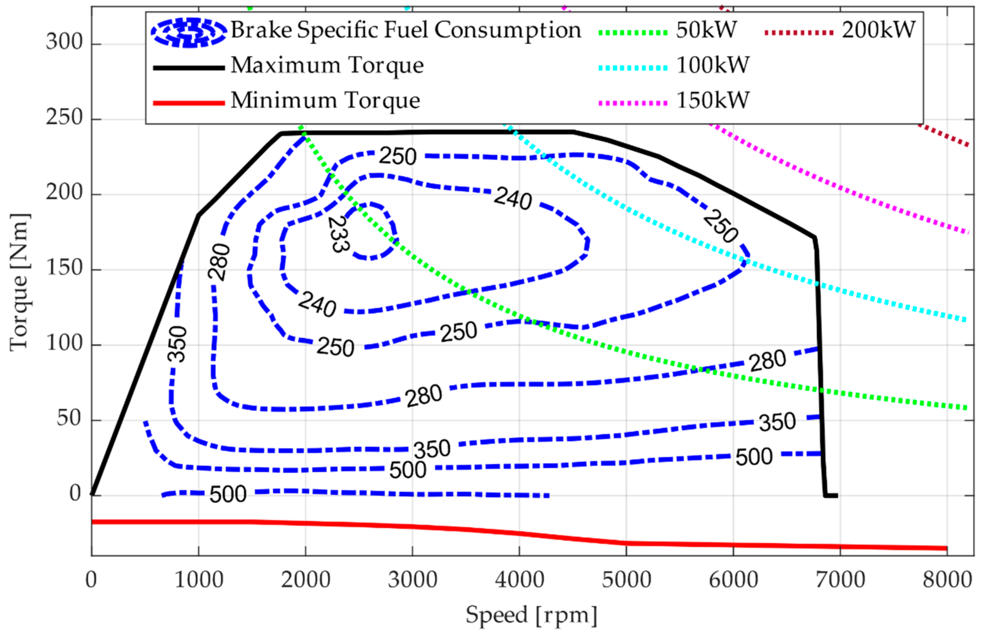
The purpose of computing an eco-driving cycle is to optimize the vehicle speed trajectory subjected to specific constraints so that the total energy consumption is minimized. In the case of a conventional vehicle, the idea is to minimize the total fuel consumption and the sum of the positive acceleration for the fixed travel duration [7,16]. Figure 3 represents a petrol engine consumption map for a typical passenger vehicle. In the optimization algorithm, the fuel consumption is estimated using Figure 3 as a kind of lookup table. The computation of the optimal speed trajectory is calculated for a specific travel duration, subjected to the specific vehicle and environmental constraints such as speed limits, acceleration limits, and traffic constraints [4]. However, for reducing the implementation complexities, constraints subjected to external factors, such as thermal, vibration, and frictional effects, are not considered. This method of optimization formulation is often regarded as an optimal control problem (OCP) [17].

In the proposed OCP, the idea is to minimize the cost function so that the optimal energy consumption is achieved. In this work, the minimization cost function is defined as:

$$J=\frac{\beta }{{\lambda }_{\dot{m}}}*{{\displaystyle \int }}_0^{t_f}\dot{m}\left({\omega }_e\left(t\right),T_e\left(t\right)\right)*dt+\frac{\left(1 - \beta \right)}{{\lambda }_a}*{{\displaystyle \int }}_0^{t_f}a\left(t\right)*dt, where \dot{m}\left(t\right)\ge 0 and a\left(t\right)\ge 0$$

(11)

Therefore, the OCP can be written as:

$$\left(\mathrm{OCP}\right): \underset{J}{\min }\left(\frac{\beta }{{\lambda }_{\dot{m}}}*{{\displaystyle \int }}_0^{t_f}\dot{m}\left({\omega }_e\left(t\right),T_e\left(t\right)\right)*dt+\frac{\left(1 - \beta \right)}{{\lambda }_a}*{{\displaystyle \int }}_0^{t_f}a\left(t\right)*dt\right)$$

(12)

Equation (11) combines both the sum of fuel consumption $\dot{m}\left({\omega }_e\left(t\right),T_e\left(t\right)\right)$ in kg/s and the sum of positive acceleration $a\left(t\right)$ in m/s² of the vehicle by introducing the weight factor $\beta$. The tunable weight factor $\beta$ controls the influence between fuel consumption and velocity fluctuations to the cost function, so the performance of the optimization can be adjusted by varying the weight factor. Both sums in the cost function are normalized with ${\lambda }_{\dot{m}}$, and ${\lambda }_a$. The sum of positive acceleration also serves as one of the driver comfort factors by reducing the number of jerks, in addition to a comparative influence in reducing the overall net fuel consumption [16]. Though there are many other approaches to deal with the speed fluctuations [13], this research focuses on the OCP cost function defined in Equation (12), which incorporates the weighted sum of positive acceleration for the implementation of the optimization algorithm.

In Equation (12), ${\omega }_e\left(t\right)$ and $T_e\left(t\right)$ are the control variables to be optimized by varying the velocity $v\left(t\right)$. For a specific vehicle, the engine speed, the engine torque, and the gear-box ratios are physically limited to specific values. Therefore, the optimization for the eco-driving cycle is computed under mixed state and input constraints to the vehicle.

The input and the mixed state constraints for the OCP related to the vehicle limitation, and the speed limits, are listed as follows:

$$v\left(x\right)\in \left[0, v_{max}\left(x\right)\right]$$

(13)

$$a\left(t\right)\in \left[a_{min},a_{max}\right]$$

(14)

$$T_e\left(t\right)\in \left[0,T_{max}\right]$$

(15)

$${\omega }_e\left(t\right)\in \left[0,{\omega }_{max}\right]$$

(16)

$$x\left(t_f\right)=D$$

(17)

$$v\left(t_f\right)=v_f$$

(18)

$$t\left(D\right)= t_f$$

(19)

Equation (13) limits the speed of the vehicle $v_{max}\left(x\right)$ with respect to the vehicle position. To induce the speed limit for the standard driving cycles, a fixed limit margin of $e_l$ on the input driving cycle $v_{ref}\left(x\right)$ is used. The fixed margin varies based on real-world scenarios such as geographic limits, rules, and regulations, etc. The speed limit function is defined as:

$$v_{max}\left(x\right)=\left\{\begin{array}{c}{v}_{ref}\left(x\right)+e_l, v_{ref}\left(x\right)>0\\ 0, v_{ref}\left(x\right)\le 0\end{array}\right.$$

(20)

The speed limit $v_{max}\left(x\right)$, given by Equation (20), requires that the number of vehicles stops in the eco-driving cycle must be the same as that of the input driving cycle [4]. Other methods to assign speed limits can also be considered [18,19]. For instance, the speed limit values can be given by external or internal sources such as an intelligent transportation system (ITS), advanced GNSS, and on-board vehicular sensors. Equation (14) limits the vehicle acceleration to its physical minimum $a_{min}$ and maximum $a_{max}$. For simplicity, the maximum acceleration limit used in this paper is fixed based on few widely used standard driving cycles such as the NEDC, the Common Artemis Driving Cycles (CADC) (Urban), and the Worldwide Harmonized Light Vehicles Test Cycles (WLTC) (Class 3b). From the fuel map in Figure 3, Equations (15) and (16) limit the maximum engine torque $T_{max}$ and engine speed of the vehicle to its physical maximum ${\omega }_{max}$. Equations (17)–(19) manage the optimal eco-driving which makes the total travel distance $D$, final speed $v_f$, and the total travel time $t_f$ to the same values as those of the input driving cycles.

4. Design of Genetic Algorithm-based Solution Methodology

The OCP problem defined by Equation (12) can be approached by many global optimization solving methods such as DP, the Pontryagin minimum principle (PMP), and genetic algorithms (GA). Although DP-based methods always gives the best solution, the computational time increases exponentially with the increase in problem dimensions and thus requires the implementation of additional independent tuning parameters to reduce the problem dimension within a certain error margin [13]. Due to the non-linear nature of the OCP and the mixed state-input constraints, the formulation of the PMP is more complicated [20,21,22]. The GA-based algorithm, like any other heuristic-based global optimization algorithm, does not guarantee the best optimal solution and depends on the initialization parameters. However, the GA has a low implementation complexity and computational time, sometimes used along with other deterministic algorithms [18,23]. Thus, the method proposed here is based on the genetic algorithm.

4.1. Genetic Algorithm-based Optimization Method

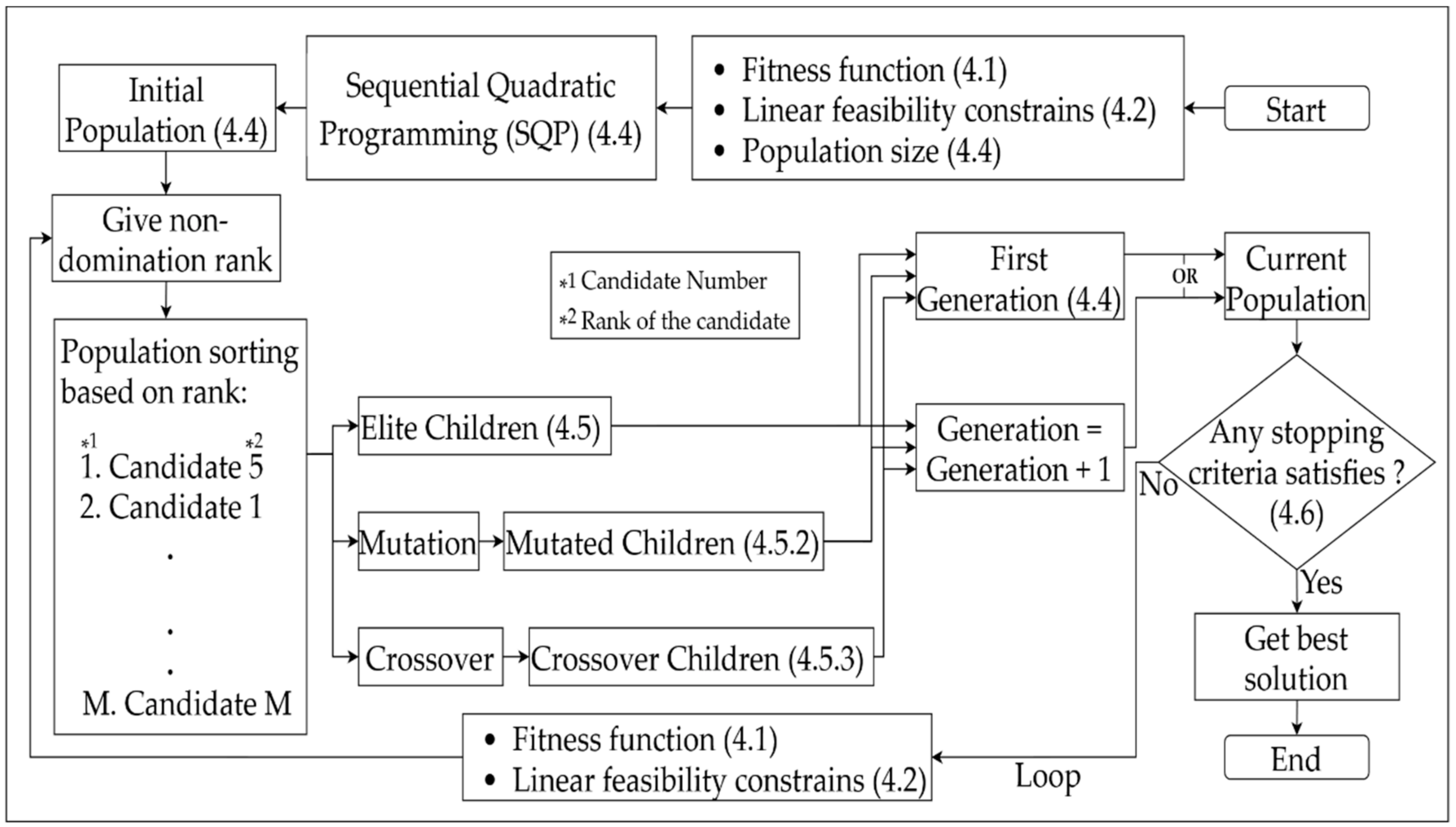
A constrained genetic algorithm (GA) is used in this paper and considers mixed linear constraints for optimizing the vehicle speed [24]. Figure 4 represents the general workflow of the GA. The fitness function of the GA is the OCP is defined in Equation (12), where time $t$ in seconds ranges from $k=1:N$ fixed steps. The GA implementation in this paper maintains a fixed population of size $M$ for every generation, and the best candidate from the last generation is selected as the final optimal solution.

4.2. Linear Feasibility Constraints

The OCP linear constraints, defined in Equations (13) and (14), are formulated as feasibility constraints for the genetic algorithm as given in Equations (21) and (22). The OCP linear constraints defined in the Equations (17) and (18) are formulated as feasibility constraints with fixed tolerances $I_{Tol}=2\%$ and $J_{Tol}= 0.2\%$, respectively, in Equations (23)–(26) [15]. The OCP constraint Equations (15) and (16) are formulated as saturation functions, i.e., the functions replace the values exceeding limits by the limit values. Any candidate from a generation not satisfying these constraints within constraint violation tolerance $V_{Tol}$ are excluded, where $V_{Tol}\in \left[0,1\right]$, in this work $V_{Tol}$, is fixed to 1e⁻⁶.

$$0\le v\left(k\right)\le v_{max}\left(k\right)$$

(21)

$$a_{min}\le a\left(k\right)\le a_{max}$$

(22)

$$C_{upper}^1\le V_{Tol}, where C_{upper}^1= {{\displaystyle \sum }}_{k=1}^{k=N}\left(v\left(k\right)*\mathrm{∆}t\left(k\right)\right)-\left(\left(I_{Tol}*D\right)+D\right)$$

(23)

$$C_{lower}^1\le V_{Tol}, where C_{lower}^1= \left(D-\left(I_{Tol}*D\right)\right)-{{\displaystyle \sum }}_{k=1}^{k=N}\left(v\left(k\right)*\mathrm{∆}t\left(k\right)\right)$$

(24)

$$C_{upper}^2\le V_{Tol}, where C_{upper}^2= v\left(N\right)-\left(\left(J_{Tol}*v_0\right)+v_f\right)$$

(25)

$$C_{lower}^2\le V_{Tol}, where C_{lower}^2 = \left(v_f-\left(J_{Tol}*v_f\right)\right)-v\left(N\right)$$

(26)

4.3. Solution Candidate Representation

Each element in a candidate is represented as a double precession floating-point number, where each element corresponds to one velocity data point. Therefore, the total number of discretized velocity datapoints $N$ is equal to the length of the chromosome. The total number of candidates in a generation is fixed to $M$, and Equation (27) shows a generic representation of a population matrix. Though operation on each floating-point array candidate requires more computing resources compared to a binary bits array candidate, this eliminates certain implementation complexities pertaining to encoding and decoding schemes.

$$S_{MN}= \left[\begin{array}{ccccccc}{v}_{11}& v_{12}& v_{13}& .& .& .& v_{1N}\\ v_{21}& v_{22}& v_{23}& .& .& .& v_{2N}\\ v_{31}& v_{32}& v_{33}& .& .& .& v_{3N}\\ \begin{array}{c}.\\ .\\ .\end{array}& \begin{array}{c}.\\ .\\ .\end{array}& \begin{array}{c}.\\ .\\ .\end{array}& & & & \begin{array}{c}.\\ .\\ .\end{array}\\ v_{M1}& v_{M2}& v_{M3}& .& .& .& v_{MN}\end{array}\right]$$

(27)

4.4. Initialization of Population

The population for the first-generation of the GA is generated by minimizing the OCP function using a local minimization algorithm, therefore enabling a reasonably large and diverse initial solution space for the GA optimization to find an optimal solution close to the ideal true global value [18]. Sequential quadratic programming (SQP) [25,26,27,28,29,30] is used to create an initial population of size $M$ subjected to the same set of constraints and fitness functions defined previously. The SQP tries to generate feasible candidates from a variety of pseudorandom initial data points. Figure 5 shows an example of the initial population for the EUDC with the population size $M=25$ and discreet velocity points $N=102$.

4.5. Evolution Strategies for the Proposed GA

Similar to other evolutionary algorithms, in GAs, the operations are applied in a loop with modifications performed during every iteration. In this work, modifications are performed using selection, mutation, and crossover functions on candidates at every generation. At each generation, three types of children are produced, namely, the elite, the crossover, and the mutation children. The density or number of children corresponding to a particular type is controlled by the predefined ratio of $Q_e$, $Q_c$, and $Q_m$ such that the size of the population remains the same as defined in Equation (28). $Q_e$ multiplied by $M$ candidates from the previous generation are selected as the elite children for the next generation based on the fitness function value. The other two types of children are created by mutation and crossover functions with the help of a tournament-based selection method used to choose parents.

$$M= Q_e*M+Q_c*M+Q_m*M, where Q_e+Q_c+Q_m=1$$

(28)

4.5.1. Selection Method

A tournament selection is used for the selection of candidates from the previous generation to be parents for the next generation. In the tournament method, a random fixed number of candidates is picked, and then the best candidate from that fixed set of candidates is selected to be the parent for the next generation. In this work, both the mutation function and crossover function select parents using the tournament selection method, and the fixed number of candidates for selection is set to four.

4.5.2. Mutation Function

A mutation is performed on a single parent, and random changes are applied to that parent to produce children. Equation (29) shows an example candidate matrix with the mutated chromosomes emphasized. An adaptive mutation function is used in this work that produces $Q_m$ multiplied by $M$ children for the next generation. The mutation function randomly selects the step length and direction based on the last successful or unsuccessful generation so that all the children produced by the mutation function always satisfy the linear feasibility constraints.

$$Chil{d}_1= \left[v_{11}, v_{12}^{’}, v_{13}, v_{14}^{’}, v_{15}, v_{16}, v_{17}^{’}, v_{18}, \dots , v_{1N}\right]$$

(29)

4.5.3. Crossover Function

A crossover operation is performed using two candidates from the previous generation as parents; each child is unique and inherits different traits from both parents. In this work, the crossover function creates children equal to the random weighted arithmetic mean of both the parents, as shown in Equation (30). The total number of crossover children is equal to $Q_c$ multiplied by $M$.

$$Chil{d}_2=Random*Paren{t}_A+\left(1-Random\right)*Paren{t}_B, where Random\in \left[0,1\right]$$

(30)

4.6. GA Stopping Criteria

The genetic algorithm runs in the form of a loop with an incrementing generation. The loop is terminated and the best solution from the last generation is selected as the final solution, if any of the three conditions are satisfied:

• The total number of generations exceeds the specified limit $Ge{n}_{lim}$
• The total number of stall generations exceeds the specified limit $Stal{l}_{lim}$, a generation is considered as a stall generation when the average change in the fitness function value is less than the fixed tolerance $H_{Tol}$
• The total computation time exceeds the specified limit $Tim{e}_{lim}$.

5. Analysis and Results

The OCP optimization is performed on several widely used driving cycles such as the Common Artemis Driving Cycles (CADC—Urban and CADC—Road), the Worldwide Harmonized Light Vehicles Test Cycles (WLTC)—Class 3b, the Federal Test Procedure (FTP-75), the Supplemental Federal Test Procedure (SFTP)—US06, the New European Driving Cycle (NEDC), the RTS Aggressive or RTS 95, California Unified Cycle (UC), the Highway Fuel Economy Test (HWFET or HFET), and the EPA New York City Cycle (NYCC). The optimization is carried out using the OCP defined in Equation (12) and using the genetic algorithm discussed previously. The optimal eco-driving cycles from the optimization algorithm are fed to and simulated with the virtual vehicle model to get the fuel consumption. Figure 6 shows the percentage reduction in fuel consumption with respect to the initial driving cycle for various weight factors, and the percentage value is corrected in a way that, if fuel consumption from the optimal eco-driving cycle exceeds the initial cycle, then the percentage reduction in fuel consumption is considered zero. The optimal value for the weight factor $\beta =0.5$ is selected, based on the average of the weight factors fitting to the maximum improvement in terms of the percentage reduction in fuel consumption for the various standard driving cycles.

Figure 7 show the optimal eco-driving cycle computed for the WLTC—Class 3b. The reduction in fuel consumption is achieved mainly by the changes in the driving actions such as reduced accelerations, maximum velocities, number of speed fluctuations and likewise, some of these changes are highlighted in the Figure 7 and the same can also be observed in Figure 8 and Figure 9.

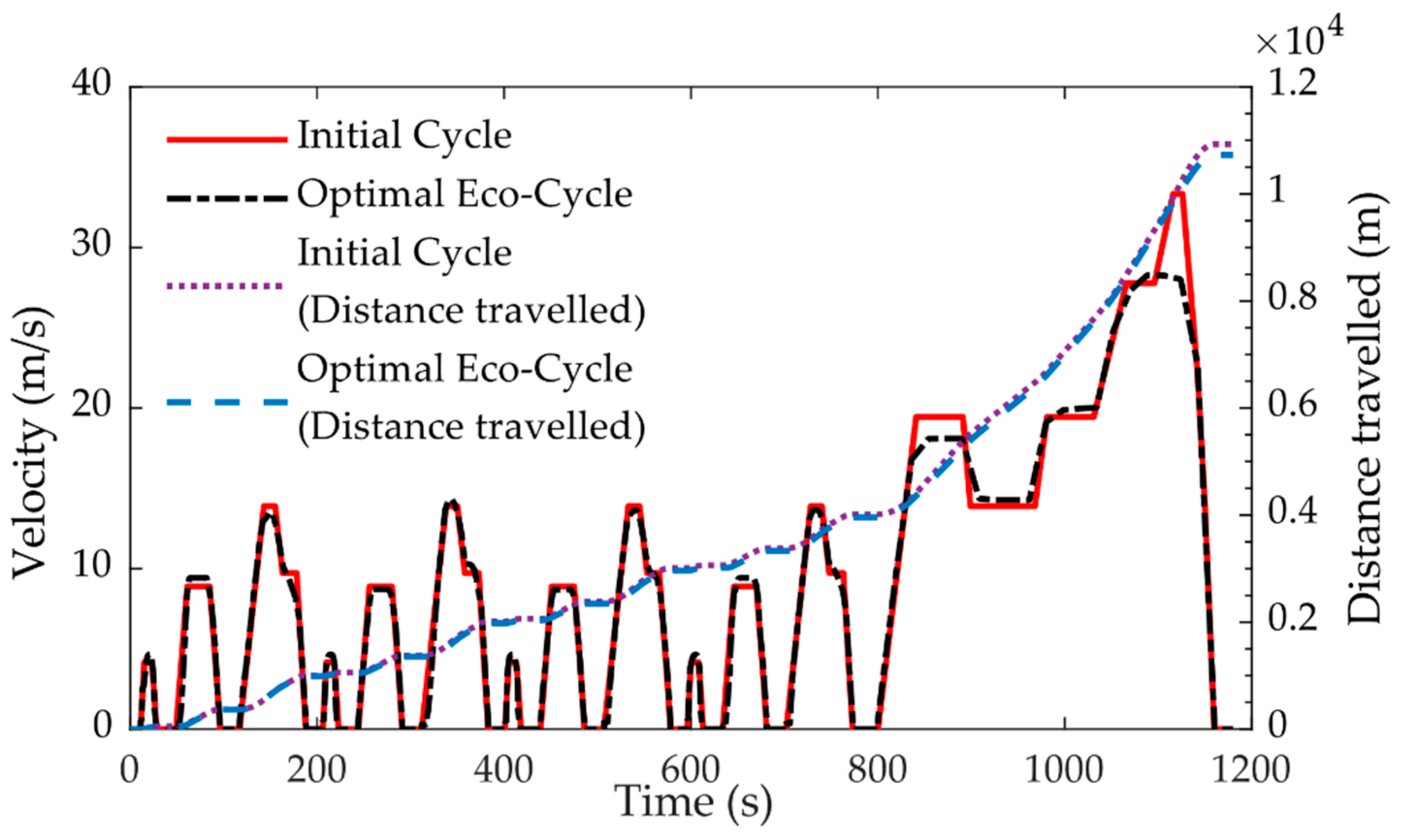
Figure 8 shows the eco-driving cycle computed for the NEDC and Figure 9 displays the optimal eco-driving cycle computation for a simulated real-world driving cycle, pertaining to an area in RWTH Aachen University, Nordrhein-Westfalen, Aachen, Germany. The velocity data is acquired by microscopic traffic simulation software.

Table 1. Optimization results for different driving cycles.

Driving Cycles	Initial (L/100 km)	Optimized Results
		L/100 km	% Fuel Reduction
NEDC	6.63	6.03	9.05
WLTC3b	6.39	5.76	9.86
Artemis-Urban	9.11	8.47	7.03
Artemis-Road	5.75	5.04	12.35
FTP75	6.24	6.05	3.04
Simulated real-world	6.01	5.45	9.32
Average	-	-	8.44

¹ For all driving cycles in the table, weight factor $\beta =0.5$ is used.

represents the fuel reduction of the computed optimal eco-driving compared with the initial cycle, and the results show that an average reduction of eight percent in fuel consumption is achieved. One of the conclusions drawn is that the algorithm works more effectively in high-speed compared to low-speed areas.

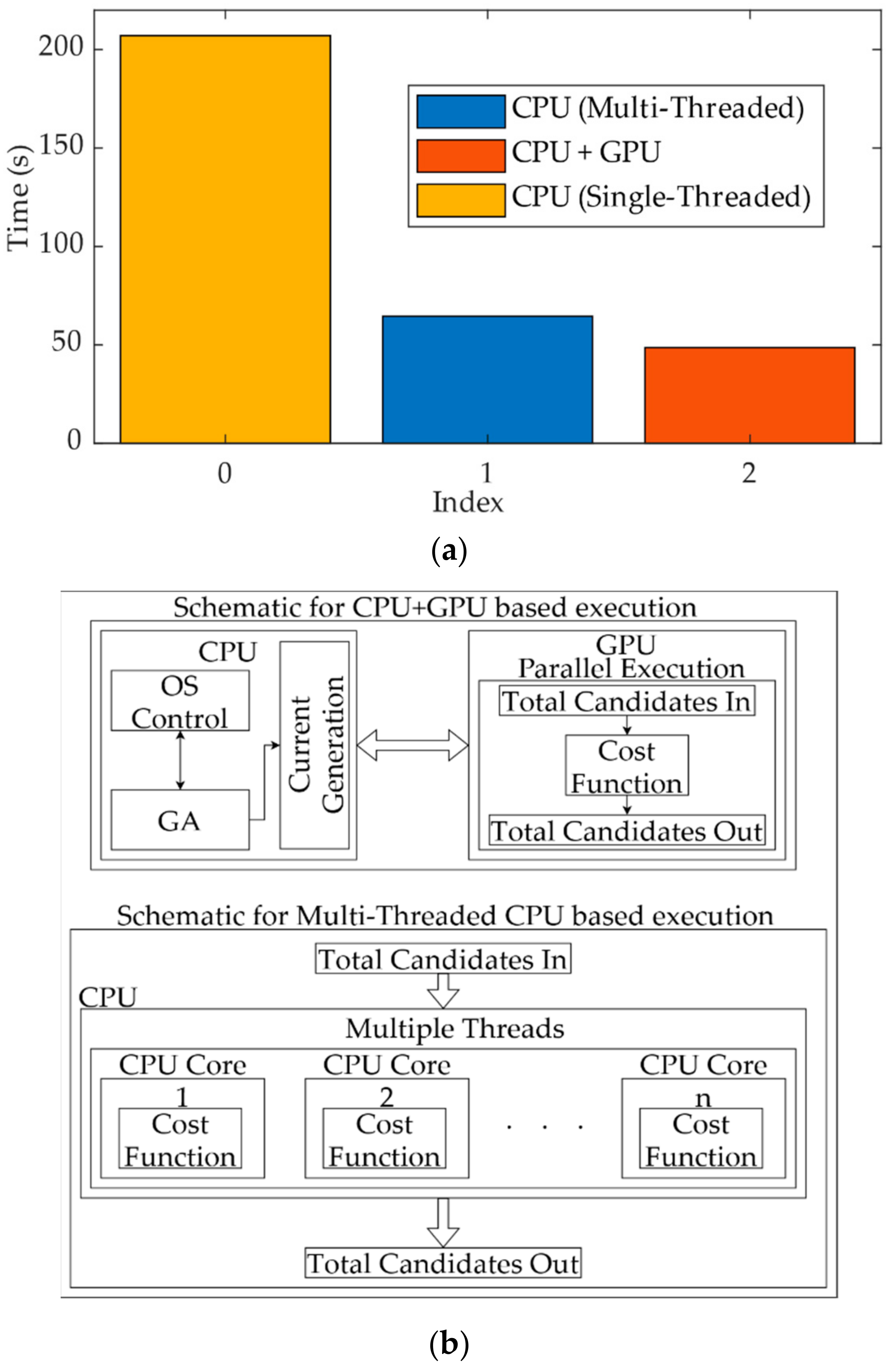
One of the main advantages of the proposed method of optimization is that the total memory requirement of the computing device is less compared to the DP algorithm, since at every iteration, unlike the DP, the GA deletes the poor candidates and thus reduces the search space. Another advantage is that every chromosome in the proposed GA is independent to from the others and thus gives the possibility of scaling the computation across multiple computing resources in parallel. Figure 10 illustrates the advantages of parallelization in computing the cost for all the candidates in a generation at the same time, and from Figure 10a the GA execution time is compared with the single-threaded CPU (central processing unit), the multi-threaded CPU, and the CPU+GPU (graphics processing unit)-based implementation. The generic execution flow of the multi-threaded CPU and the CPU+GPU-based implementation is illustrated in Figure 10b.

For the CPU only calculation, a 48 core Intel Skylake Platinum 8160 with a clock speed of 2.1 GHz is used, and for the GPU, one Nvidia Tesla V100 is used. For all three types, the same initial population is used, and the OCP is converted to a distance-based function using interpolation, similar to the work done by D. Maamria et al. [13].

6. Conclusions

The computation of eco-driving cycles for vehicles fitted with internal combustion engines is addressed and formulated as an optimal control problem by considering both the fuel consumption and driver comfort of the vehicle. The proposed method is performed on several widely used standard driving cycles, and a simulated real-world driving cycle, and the results show that an average reduction of eight percent in fuel consumption is achieved, while the algorithm works more effectively in high-speed compared to low-speed areas of the driving cycles. The cost function calculation part of the proposed GA is parallelized on different computing hardware and the outcomes indicate that the execution efficiency can be improved based on the availability of the computing resources.

The idea is that the proposed optimization method can be adopted onto a cloud-based cluster computing system, where the environmental constraints, such as traffic conditions, vehicle specific limitations, and likewise, are fed to the optimization algorithm in real-time, and so the results can then be communicated to the vehicle or driver to improve fuel consumption. The robustness of the proposed optimization methodology to deal with appreciable uphill and/or downhill paths in the route, has been ascertained through the gradient resistance component of the vehicle model proposed. However, in an ideal case of network connected autonomous vehicles, the percentage reduction in fuel consumption can further be improved, since some of the effects related to the behaviors of human drivers, such as parallax errors, comfort preferences, travel time forbearances and likewise, are minimized.

It is planned in a future study to take the predictive horizon into account, as this will enable the possibility of using the proposed method in the on-line optimization with a fixed look-ahead distance or time. This work can also be extended to an electric vehicle, where the mass flow rate $\dot{m}$ is replaced with electric power, and the vehicle energy demand can be modeled in terms of the state of charge (SOC) while replacing the integrated fuel map of the internal combustion engine with the efficiency map of the electric motor.

7. Definitions of Notations

The following

Table 2. Definitions of notations used in vehicle modeling.

Notation	Definition	Unit
$a\left(t\right)$	Acceleration	m/s2
g	Acceleration due to gravity	m/s2
$C_{air}$	Coefficient of aerodynamic drag	-
$C_{roll}$	Coefficient of rolling resistance	-
$\rho$	Density of air	kg/m3
$R_d$	Differential ratio	-
${\eta }_{dt}$	Drivetrain efficiency	-
$r_{tire}$	Dynamic wheel radius	m
$I_e$	Engine inertia	kgm2
${\omega }_e\left(t\right)$	Engine speed	rad/s
$T_e\left(t\right)$	Engine torque	Nm
A	Frontal area	m2
$R_{gb}\left(t\right)$	Gear-box ratio	-
$\theta \left(t\right)$	Gradient angle	rad
$v_0$	Initial velocity	m/s
$N_{wh}$	Number of wheels	-
$x\left(t\right)$	Position	m
$F_R\left(t\right)$	Resistive force	N
t	Time	s
$F_T\left(t\right)$	Traction force	N
m	Vehicle mass	kg
$v\left(t\right)$	Velocity	m/s
$I_{wh}$	Wheel inertia	kgm2
${\omega }_{wh}\left(t\right)$	Wheel speed	rad/s
$T_{wh}\left(t\right)$	Wheel torque	Nm

shows the nomenclature and the unit system used for the mathematical modeling of the vehicle dynamics used in this paper.

References

- Yang, Y.; Zhong, Z.; Wang, F.; Fu, C.; Liao, J. Real-time Energy Management Strategy for Oil-Electric-Liquid Hybrid System based on Lowest Instantaneous Energy Consumption Cost. Energies 2020, 13, 784. [Google Scholar] [CrossRef] [Green Version]
- Ozatay, E.; Ozguner, U.; Michelini, J.; Filev, D. Analytical Solution to the Minimum Energy Consumption Based Velocity Profile Optimization Problem with Variable Road Grade. IFAC Proc. Vol. 2014, 47, 7541–7546. [Google Scholar] [CrossRef] [Green Version]
- Hellström, E.; Åslund, J.; Nielsen, L. Design of an efficient algorithm for fuel-optimal look-ahead control. Control Eng. Pract. 2010, 18, 1318–1327. [Google Scholar] [CrossRef] [Green Version]
- Mensing, F.; Bideaux, E.; Trigui, R.; Ribet, J.; Jeanneret, B. Eco-driving: An economic or ecologic driving style? Transp. Res. Part C Emerg. Technol. 2014, 38, 110–121. [Google Scholar] [CrossRef]
- Hellström, E.; Ivarsson, M.; Åslund, J.; Nielsen, L. Look-ahead control for heavy trucks to minimize trip time and fuel consumption. Control Eng. Pract. 2009, 17, 245–254. [Google Scholar] [CrossRef] [Green Version]
- Passenberg, B.; Kock, P.; Stursberg, O. Combined time and fuel optimal driving of trucks based on a hybrid model. In Proceedings of the 2009 European Control Conference (ECC), Budapest, Hungary, 23–26 August 2009; pp. 4955–4960. [Google Scholar]
- Nault, E.; Colin, G.; Gillet, K.; Chamaillard, Y.; Zerar, M.; Dollinger, N.; Nouillant, C. Towards an Analytical Eco-Driving Cycle Computation for Conventional Cars. IFAC PapersOnLine 2019, 52, 550–555. [Google Scholar] [CrossRef]
- Silvas, E.; Hofman, T.; Murgovski, N.; Etman, P.; Steinbuch, M. Review of Optimization Strategies for System-Level Design in Hybrid Electric Vehicles. IEEE Trans. Veh. Technol. 2016, 66, 57–70. [Google Scholar] [CrossRef] [Green Version]
- Liu, X.; Ma, J.; Zhao, X.; Zhang, Y.; Zhang, K.; He, Y. Integrated Component Optimization and Energy Management for Plug-In Hybrid Electric Buses. Processes 2019, 7, 477. [Google Scholar] [CrossRef] [Green Version]
- Kim, T.S.; Manzie, C.; Sharma, R. Two-Stage Optimal Control of a Parallel Hybrid Vehicle with Traffic Preview. IFAC Proc. Vol. 2011, 44, 2115–2120. [Google Scholar] [CrossRef] [Green Version]
- Van Keulen, T.; De Jager, B.; Foster, D.; Steinbuch, M. Velocity trajectory optimization in Hybrid Electric trucks. In Proceedings of the 2010 American Control Conference, Baltimore, MD, USA, 30 June–2 July 2010; pp. 5074–5079. [Google Scholar]
- Levermore, T.; Sahinkaya, M.; Zweiri, Y.; Neaves, B. Real-Time Velocity Optimization to Minimize Energy Use in Passenger Vehicles. Energies 2016, 10, 30. [Google Scholar] [CrossRef]
- Maamria, D.; Gillet, K.; Colin, G.; Chamaillard, Y.; Nouillant, C. Optimal Predictive Eco-Driving Cycles for Conventional, Electric, and Hybrid Electric Cars. IEEE Trans. Veh. Technol. 2019, 68, 6320–6330. [Google Scholar] [CrossRef] [Green Version]
- Xu, C.; Al-Mamun, A.; Geyer, S.; Fathy, H.K. A Dynamic Programming-Based Real-Time Predictive Optimal Gear Shift Strategy for Conventional Heavy-Duty Vehicles. In Proceedings of the 2018 Annual American Control Conference (ACC), Milwaukee, WI, USA, 27–29 June 2018; pp. 5528–5535. [Google Scholar]
- Maamria, D.; Gillet, K.; Colin, G.; Chamaillard, Y.; Nouillant, C. Optimal eco-driving for conventional vehicles: Simulation and experiment. IFAC PapersOnLine 2017, 50, 12557–12562. [Google Scholar] [CrossRef]
- Chakraborty, D.; Vaz, W.; Nandi, A.K. Optimal driving during electric vehicle acceleration using evolutionary algorithms. Appl. Soft Comput. 2015, 34, 217–235. [Google Scholar] [CrossRef]
- Petit, N.; Sciarretta, A. Optimal drive of electric vehicles using an inversion-based trajectory generation approach. IFAC Proc. Vol. 2011, 44, 14519–14526. [Google Scholar] [CrossRef]
- Felicitas, M. Optimal Energy Utilization in Conventional, Electric and Hybrid Vehicles and Its Application to Eco-Driving. Ph.D. Thesis, Institut National des Sciences Appliquées de Lyon, Lyon, France, September 2013. [Google Scholar]
- Bouvier, H.; Colin, G.; Chamaillard, Y. Determination and comparison of optimal eco-driving cycles for hybrid electric vehicles. In Proceedings of the 2015 European Control Conference (ECC), Linz, Austria, 15–17 July 2015; pp. 142–147. [Google Scholar]
- Malisani, P.; Chaplais, F.; Petit, N. An interior penalty method for optimal control problems with state and input constraints of nonlinear systems: Interior method in constrained optimal control. Optim. Control Appl. Methods 2016, 37, 3–33. [Google Scholar] [CrossRef]
- Bertsekas, D.P.; Bertsekas, D.P. Approximate dynamic programming. In Dynamic Programming and Optimal Control, 4th ed.; Athena Scientific: Belmont, MA, USA, 2012; ISBN 978-1-886529-08-3. [Google Scholar]
- Bryson, A.E. Applied Optimal Control: Optimization, Estimation, and Control; Taylor & Francis Group: New York, NY, USA, 2018; ISBN 978-1-315-13766-7. [Google Scholar]
- Tian, L.; Collins, C. An effective robot trajectory planning method using a genetic algorithm. Mechatronics 2004, 14, 455–470. [Google Scholar] [CrossRef]
- Deb, K. An efficient constraint handling method for genetic algorithms. Comput. Methods Appl. Mech. Eng. 2000, 186, 311–338. [Google Scholar] [CrossRef]
- Fletcher, R. Practical Methods of Optimization: Fletcher/Practical Methods of Optimization; Wiley & Sons: Chichester, UK, 2000; ISBN 978-1-118-72320-3. [Google Scholar]
- Ricketts, R.E. Practical optimization, Philip E. Gill, Walter Murray and Margret H. Wright, Academic Press Inc. (London) Limited, 1981. No. of pages: 401. Price £19.20, $46.50. ISBN: 0.12.283950.1. Int. J. Numer. Methods Eng. 1982, 18, 954. [Google Scholar] [CrossRef]
- Powell, M.J.D. Variable Metric Methods for Constrained Optimization. In Mathematical Programming: The State of the Art; Bachem, A., Korte, B., Grötschel, M., Eds.; Springer: Berlin/Heidelberg, Germany, 1983; pp. 288–311. ISBN 978-3-642-68876-8. [Google Scholar]
- Hock, W.; Schittkowski, K. A comparative performance evaluation of 27 nonlinear programming codes. Computing 1983, 30, 335–358. [Google Scholar] [CrossRef]
- Spellucci, P. A new technique for inconsistent QP problems in the SQP method. Math. Methods Oper. Res. 1998, 47, 355–400. [Google Scholar] [CrossRef]
- Tone, K. Revisions of constraint approximations in the successive QP method for nonlinear programming problems. Math. Program. 1983, 26, 144–152. [Google Scholar] [CrossRef]
Figure 1.
Static gear shift map.
Figure 2.
Comparison of the rule-based and the lookup table-based gear shift curve for the extra-urban driving cycle (EUDC) driving cycle.
Figure 3.
Fuel consumption (g/kWh) of a petrol engine, represented as a function of the engine speed and engine torque. For confidentiality reasons, the values are normalized.
Figure 4.
Genetic algorithm implementation for the optimal control problem (OCP).
Figure 5.
Example initial population generated by sequential quadratic programming (SQP) for the EUDC.
Figure 6.
Percentage reduction in fuel consumption with respect to the initial driving cycle for various weight factors.
Figure 7.
Optimized speed trajectory for the Worldwide Harmonized Light Vehicles Test Cycles (WLTC)—Class3b ( = 0.5).
Figure 8.
Optimized speed trajectory for the New European Driving Cycle (NEDC) ( = 0.5).
Figure 9.
Optimized speed trajectory for the simulated real-world driving cycle ( = 0.5).
Figure 10.
Genetic algorithm implementation workflow: (a) GA execution time for a simulated real-world cycle; (b) schematic for CPU+GPU, and multi-threaded CPU-based implementation.