Combined Diagnostic Analysis of Dynamic Combustion Characteristics in a Scramjet Engine


Department of Aerospace Engineering, Pusan National University, Busan 46241, Korea
*
Author to whom correspondence should be addressed.
Energies 2020, 13(15), 4029; https://doi.org/10.3390/en13154029
Submission received: 19 June 2020
/
Revised: 22 July 2020
/
Accepted: 28 July 2020
/
Published: 4 August 2020
(This article belongs to the Special Issue Scramjet and Ramjet Combustion)
Abstract
:In this work, the dynamic combustion characteristics in a scramjet engine were investigated using three diagnostic data analysis methods: DMD (Dynamic Mode Decomposition), STFT (Short-Time Fourier Transform), and CEMA (Chemical Explosive Mode Analysis). The data for the analyses were obtained through a 2D numerical experiment using a DDES (Delayed Detached Eddy Simulation) turbulence model, the UCSD (University of California at San Diego) hydrogen/oxygen chemical reaction mechanism, and high-resolution schemes. The STFT was able to detect that oscillations above 50 kHz identified as dominant in FFT results were not the dominant frequencies in a channel-type combustor. In the analysis using DMD, it was confirmed that the critical point that induced a complete change of mixing characteristics existed between an injection pressure of 0.75 MPa and 1.0 MPa. A combined diagnostic analysis that included a CEMA was performed to investigate the dynamic combustion characteristics. The differences in the reaction steps forming the flame structure under each combustor condition were identified, and, through this, it was confirmed that the pressure distribution upstream of the combustor dominated the dynamic combustion characteristics of this scramjet engine. From these processes, it was confirmed that the combined analysis method used in this paper is an effective approach to diagnose the combustion characteristics of a supersonic combustor.
1. Introduction
In a supersonic combustor, which sustains highly turbulent, compressible, and non-premixed reacting flows, combustion is mostly held at the fuel/air mixing layer. Moreover, supersonic combustion is essentially an unsteady combustion with ignition, extinction, and re-ignition occurring repeatedly. The flow-residence time of a supersonic combustor with the abovementioned features is very short, in the order of 1 ms. This implies that all the processes of mixing, ignition, and combustion after the fuel is injected must take place within an extremely short time span. Thus, flame holding, which avoids extinction and propellant mixing, is recognized as one of the most important mechanisms in supersonic combustion. As with all other combustors, supersonic engines also exhibit different combustion characteristics depending on the shape of the cavity and the combustor, the working fluid, and the operating environment.
Choi et al. [1,2] provide a well-elaborated numerical experiment that was conducted to identify combustion characteristics depending on various shapes and injection pressures under the same operating condition. This study confirmed the dynamic combustion characteristics of the unsteady behavior inside a supersonic combustor according to a combination of several conditions, such as expansion angle, cavity, and the transverse fuel injection pressure. Gerlinger et al. [3] conducted a numerical experiment for fuel mixing and combustion enhancement using a strut-type injector. In this study, it was found that the mixing efficiency of a lobed strut is higher than that of a planar strut but has larger increases in entropy and total pressure losses. Choi et al. [4] and Li et al. [5,6] conducted a numerical study on the transient process of ethylene fuel injection into a direct-connect dual-mode scramjet combustor with air throttling. In these works, the effect of air throttling for the ethylene ignition and combustion establishment was identified with the transient process of this combustor. Bermejo-Moreno et al. [7] studied the combustion characteristics during the transition from dual- to scram-mode by imposing a change in the operating and injection conditions. This study confirmed that oscillations in the recirculating area formed at the primary injection point in the scram-mode affect fuel mixing. Larsson et al. [8] conducted a study on the reacting flow for increased fuel/air equivalence ratios in a HyShot II scramjet combustor. This numerical study, which also involved the validation of an equilibrium wall model and a flamelet-based combustion model, detected quantitative changes at an equivalence ratio of 0.39. Hwang et al. [9] performed a numerical experiment to investigate the effects of fuel temperature on the characteristics of supersonic combustion. This work confirmed that fuel and air are burnt when mixing at high temperatures, whereas a partially premixed mixture is preserved in low fuel temperatures. In addition to these studies, several other numerical studies have been conducted on supersonic combustors and provide insightful results to understand the supersonic combustion phenomenon. Liu et al. [10] carried out a numerical study of cavity-stabilized hydrogen combustion in a one-sided diverging combustor by large eddy simulation coupled with an assumed PDF (Probability Density Function) model. In this work, through three-dimensional numerical analysis with about 70 million grid resolution, the flame structure and fuel mixing characteristics of each region of the combustor were identified. Moradi et al. [11] conducted a comprehensive numerical experiment to investigate the geometric effect of the cavity shape on the fuel mixing characteristics in a supersonic combustor with hydrogen injection. Two-dimensional numerical analysis was performed on the three shapes: circle, rectangular, and trapezoidal cavity. They obtained results that the trapezoidal cavity is the most efficient for the generation of the wide and stable ignition point. Also, it was revealed that the flow of fuel is more stable in downstream of the trapezoidal cavity rather than other geometries in a high injection–pressure ratio. Edalatpour et al. [12] studied the impact of a multi-hydrogen jet inside the cavity on a fuel mixing of supersonic flow. This study founded that the increase of the momentum of the fuel jet significantly increases the mixing rate inside the cavity, and the rising of the freestream Mach number decreases the mixing zone inside the cavity.
In addition to the cases mentioned above, many research groups are conducting a numerical study to identify a characteristic of the reacting flow field in a variety of supersonic combustors using different approaches. These numerical studies conducted on various approaches and conditions mostly have one common thing. Most of these studies have analyzed the results with the spatial distribution of physical quantities and each species concentration obtained by numerical experiments or values, such as the flame index, scalar dissipation rate, and mixture fraction, which are calculated by these physical quantities. At this point, there is a need to question whether a specific point of time or the averaged result can properly represent the dynamic characteristics of the combustor. Especially, each part of a supersonic engine, such as the main combustor, injector, cavity, isolator, and intake, strongly influences each other’s dynamic combustion characteristics. Therefore, it is necessary to try to investigate the behavior of a continuous time period in addition to an instantaneous or time-averaged result.
In this situation, several methods that can be classified as a postprocessing tool have been developed to better understand the detailed flame structure or unsteady behavior of the system. Of these methods, the first method used in this study is the STFT (Short-Time Fourier Transform) [13]. Conventionally, the FFT (Fast Fourier Transform) is used as a technique to extract the frequency-response characteristics in the system, but the limiting factor is that the frequency change based on time cannot be specified. To supplement these disadvantages, the STFT divides the entire signal of the system into short time ranges and performs a Fourier transform. Through this approach, frequency distributions for each time interval can be identified. The second method used in this study is DMD (Dynamic Mode Decomposition), which was recently proposed by Schmid [14]. This method can extract mode information that is coupled with temporal and spatial data using linear relationships between each instantaneous spatial information, called snapshot, that is essentially part of a nonlinear system. DMD has been widely used not only in the aerodynamic field but also in many other research areas [15]. In the field of aerospace propulsion, DMD has been used for the identification of combustion instability of rocket combustors [16] and the analysis of shockwave structures of a SIC (Shock Induced Combustion) system [17]. The third and last diagnostic analysis method used in this study is the CEMA, which can accurately detect flame structures [18,19]. This method based on an eigenanalysis of the chemical Jacobian has a great advantage in that it can derive chemical species and reaction steps involved in the chemical reaction of a local or entire region.
In this work, these three methods were used to identify the dynamic combustion characteristics of a scramjet engine from various perspectives and, through these characteristics, confirm the efficiency of this combined diagnostic analysis approach. First, to evaluate the frequency behavior of the scramjet engine over time, the STFT was performed according to the shape of the combustor and operating conditions. Next, to identify air–fuel mixing characteristics, which is important for supersonic combustion, the mass fraction of fuel and the pressure field data were analyzed using DMD. Lastly, CEMA was performed on a combustor with different shapes and operating conditions to compare the detailed flame structures formed under each condition and identify how the dynamic characteristics according to that condition affect the chemical kinetics. To acquire the numerical data, a two-dimensional numerical experiment was performed using the DDES turbulence model, UCSD combustion model, and high-resolution methods. All the conditions of the numerical experiment, including the computational domain, working fluid, and shape conditions, were set to be similar to those of the previous study performed by Choi et al. [1,2].
2. Materials and Methods
2.1. Computational Model
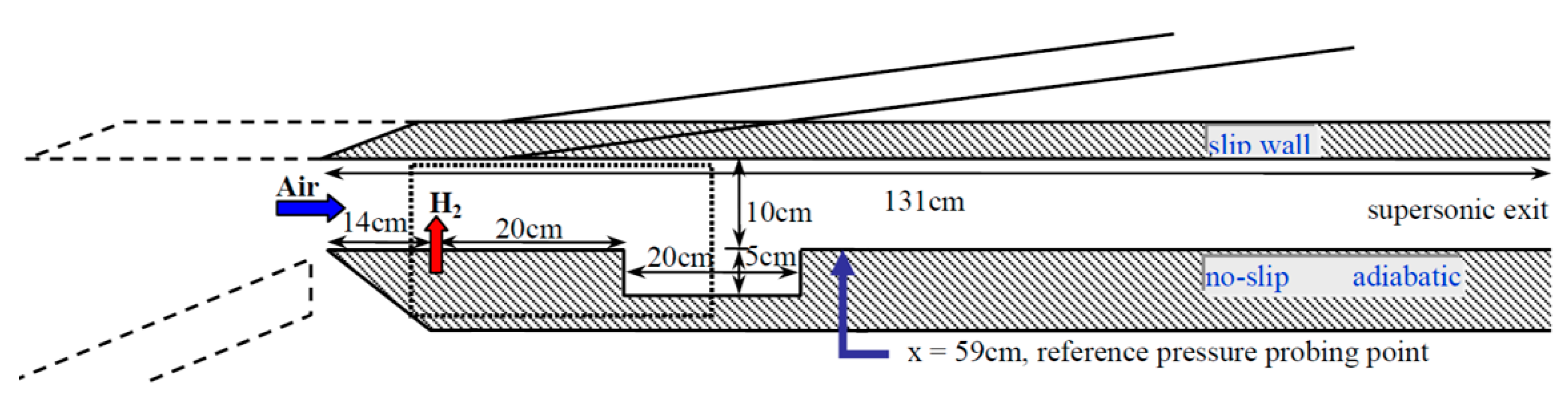
The scramjet engine used in this study is shown in Figure 1. This engine consists of a cowl under the intake, diverging nozzle or straight-channel main combustor, and cavity. Except for the cavity, this combustor is quite similar to the Hyshot test model [20]. The incoming air through the 10 cm inlet is assumed to be Mach 3.0/600 K/0.1 MPa. The fuel, which is gaseous hydrogen, is injected transversely into the main combustor through a 0.1 cm-wide choked slot injector. For the numerical experiment, three injection pressures were assumed to be 0.5/0.75/1.0 MPa, which are 5/7.5/10 times the incoming air pressure, respectively. But in each section of this study, only a specific pressure injection case is analyzed. The gaseous hydrogen fuel temperature is assumed to be 300 K. As mentioned earlier, all the imposed conditions were set similarly to the previous study [1,2], except for the number of fuel injection pressures.
2.2. Two-Dimensional Numerical Experiment
To simulate a reacting flow field of a supersonic combustor with high accuracy, three-dimensional calculations must be performed for several reasons. One of the reasons is the side-wall effect. When side wall is considered, the effective cross-section area is reduced compared to the two- dimensional case by a wall boundary layer along the surface of the side wall. Also, the side wall generates the corner flow, which reduces the effective cross-section area. Another reason is the interaction of the upper and lower wall. The boundary layers of upper and lower walls are connected by the boundary layer of side wall. It is found that this connected boundary layer would be important for flame propagation during ignition transients [6]. The supersonic combustion is governed by the fuel/air mixing, and it is linearly dependent on the contact area. If the computational domain is expanded from two-dimensional to the three-dimensional, the surface area of the eddy is considered to be about twice as large [21]. For this reason, there is a tendency to under-predict the combustion and propulsion efficiency in two-dimensional numerical experiments.
Despite these issues, two-dimensional numerical experiments were conducted in the present study instead of three-dimensional simulation, since two-dimensional simulation still has great advantages coming from the efficiency. Considering the order of 100 grid points in a span-wise direction, two-dimensional simulation needs less than 1/100 of computational resources and time compared to three-dimensional simulation, while maintaining the same resolution. Thus, fine-resolution simulation of LES (large eddy simulation) levels is available for a full-scale supersonic combustor for the long time of operation for which full 3D LES simulation has not been very successful until now. The purpose of the present study is to compare the previous analysis results that were based on typical analysis techniques with the current analysis results used by proposed approach and to investigate the effectiveness of this approach on deriving dynamic combustion characteristics on a supersonic combustor. To achieve this purpose, it was necessary to follow the two-dimensional calculations performed in previous studies. Also, the computational model of the current study has a rectangular cross-section, so the two-dimensional modeling could be a reasonable approach.
2.3. Numerical Approach
In the two-dimensional coordinate system, continuity, momentum, energy, and chemical species conservation equations—in which the flow and chemical reaction are fully coupled—were used as the governing equations and formulated using a finite volume method. The spatial discretization of the computational domain was treated by 3rd order TVD (Total Variation Diminishing)-MUSCL (Monotonic Upstream-centered Scheme for Conservation Laws). The convective and viscous fluxes were discretized using the AUSMDV (Advection Upwind Splitting Method flux Difference and Vector splitting biased) flux-splitting scheme [22] and the 4th order central difference method, respectively. Each iteration step employing the 2nd order implicit time integration is used with sub-iterations to ensure accuracy. To describe the turbulence behavior, the SST-DDES, which is classified as a hybrid RANS (Reynolds-averaged Navier–Stokes equations /LES, was applied [23].
For the chemical model, the UCSD hydrogen/air pressure-dependent reaction mechanism [24] was selected because, in a preliminary numerical study that compared a total of six hydrogen/oxygen mechanisms [25], it most effectively simulated the combustion flow field of a SIC (Shock-Induced Combustion). The UCSD mechanism is included in Table 1. This reaction mechanism consists of 8 species (H, H2, O, O2, H2O, OH, H2O2, HO2) and 21 reaction steps. In the numerical experiment, a total of nine chemical species, including nitrogen, were used as input; however, nitrogen was assumed an inert gas due to the minor effect it has on the flame-evolution process during the oxidation process. Grid resolutions of the main combustor, cavity, and cowl were 800 × 160, 159 × 161, 50 × 50, respectively. The entire computational domain applied grid clustering near the walls to capture the boundary layer. Details of the overall framework of the in-house code called PNU-RPL(Pusan National University-Rocket Propulsion Lab.) 2D and the grid dependency used for this computational domain can be found in previous studies [1,9].
2.4. Diagnostic Analysis Methods
As previously mentioned, a point data analysis using methods such as the FFT and PSD, which are widely used, is unable to investigate the frequency behavior according to the time progress. Therefore, the first diagnostic analysis method used in this study, the STFT, can compensate for these limitations and sequentially performs FFT several times for a specific section called a window size:
where are discrete signal data for the time and frequency, respectively. is the signal data of the analysis target, is the number of discrete signal data and is the window function. The entire time range of the analysis data is divided into several window sizes and the FFT is sequentially performed by overlapping the specified time period between these window sizes. Among the many window functions developed to date, the Blackman window function, which is known to provide accurate frequency estimations with little noise, was applied.
The Blackman window function is calculated with the equation above, where is the number of signal data in the window. Although the STFT is clearly an effective analysis method and can identify the dynamic characteristics of a point data, it can only extract the characteristics of the local area. Therefore, to investigate the dynamic characteristics of not only a point data but the spatial data of the entire computational area acquired from the numerical experiment, an additional approach is required.
For this purpose, DMD was applied as the second diagnostic analysis method in this study. More specifically, SVD (Singular Value Decomposition)-based DMD, a DMD algorithm recently proposed by Schmid [14], was used for the modal decomposition of unsteady flow. With the SVD-DMD, which is based on the linear relationship between unsteady information, it is possible to extract the frequency and shape of a mode coupled with temporal and spatial information. Additionally, it provides the growth/decay rate and normalized coherence of the mode, which can facilitate the understanding of the evolution of the flow system and the relative ranking of the modes, respectively [26].
To calculate the DMD mode, the first step is to construct and matrices with column vectors as temporal information and row vectors as spatial information. If the entire analysis region consists of n snapshots, the matrices and are built with 1~(n − 1) and 2~n sequential snapshots.
Finding the eigenvalue and eigenvector of matrix which includes a linear relationship of each snapshot, is key to the DMD. For this purpose, the DMD calculation starts by conducting the SVD of matrix .
In general, the amount of spatial data is much greater than the amount of temporal data, resulting in the formation of the matrix in a rectangular form, thus performing a reduced SVD instead of a full SVD. The orthogonal matrices and consist of a left and right singular vector of matrix respectively, and the diagonal component of matrix is composed of the square root of the singular values of matrix :
Because matrix cannot be directly calculated, the projected matrix , which is matrix projected onto matrix (spatial space), is used. The eigenvalues of the projected matrix are the same as the eigenvalues of matrix . So it can be possible to express Equation (3) to the formulation of eigenanalysis, Equation (6).
As mentioned above, the purpose of DMD is to find the eigenvalues () and eigenvectors () of matrix , which contains a linear relationship of spatial information for each time in a nonlinear system. The eigenvalues () can already be obtained in Equation (6). The eigenvectors () can be obtained by multiplication eigenvectors derived from the eigenvalue decomposition of the projected matrix and the matrix containing the spatial information, obtained by reduced SVD of the matrix. The eigenvector () is the DMD mode, and it shows the shape of the DMD mode. The subscript refers to the number of the DMD mode.
Each detailed description and mathematical proof of each calculation step in the DMD process is documented in the references [14,15,16]. The frequency (), damping coefficient (), and coherence () of each mode can be calculated by using the eigenvalue. is the physical time between the snapshots and is the eigenmode of the projected matrix . When calculating coherence, it should be noted that each column of is used.
The two diagnostic analysis methods above, DMD and STFT, can be used to identify the dynamic characteristics of the reacting flow field. To identify the combustion characteristics of the combustor, it is necessary to analyze the combustion field and flame structure more closely. Until now, by analyzing the distribution of the OH and H2O mass fraction, the combustion field of the hydrogen/oxygen reacting flow has been investigated. To investigate the flame structure in more detail additionally, some parameters, such as scalar dissipation rate, flame index, and mixture fraction, have been used. However, particularly in the case of supersonic combustion with a highly compressible reacting flow, it is necessary to better understand the influence of the flow field on the flame structure. Therefore, CEMA, which can extract chemical species and chemical reactions involved in the combustion process to analyze flame structures, was applied. CEMA, the last diagnostic analysis method of this study, begins by conducting the eigenvalue decomposition of the chemical Jacobian matrix [18,19], which contains the chemical source terms based on the local state vector of the dependent variables. In essence, the Jacobian matrix for the chemical source term is organized as below.
where , , and denote the momentum component of , , , and is total energy per unit volume in this work. expresses each chemical species of the chemical reaction mechanism used in the solver. In the present work, nonchemical source terms are eliminated, because it is only interested in the chemical source term for capturing the chemical mode. Therefore, the Jacobian matrix for the chemical source term , reconstructed by partial derivative components, ~, consequentially contains only a source term for a chemical species. Eigenvalue decomposition of can determine the eigenmode associated with the eigenvalue which is the largest positive eigenvalue that can be obtained. This eigenmode is called the explosive mode. By using Equation (14), the EI (Explosive Index) can be determined using the normalized contribution of each chemical species for the reaction:
where and are the right and left eigenvectors corresponding to , respectively, and denotes element-wise multiplication. In this study, the dominant EI was also applied to identify the dominant factor of the reacting flow for the local area. Using a similar process, the PI (Participation Index), which is the contribution of each chemical-reaction step involved in the reaction process can be calculated with the following equation:
where is the stoichiometric coefficient and is the vector of the net reaction rate. Similar to the EI, through the PI, it is possible to determine the contribution of each reaction and also identify which reaction steps are dominant in the local region.
3. Analysis Results of the Numerical Experiment and Dynamic Combustion Characteristics
3.1. Numerical Experiment Results
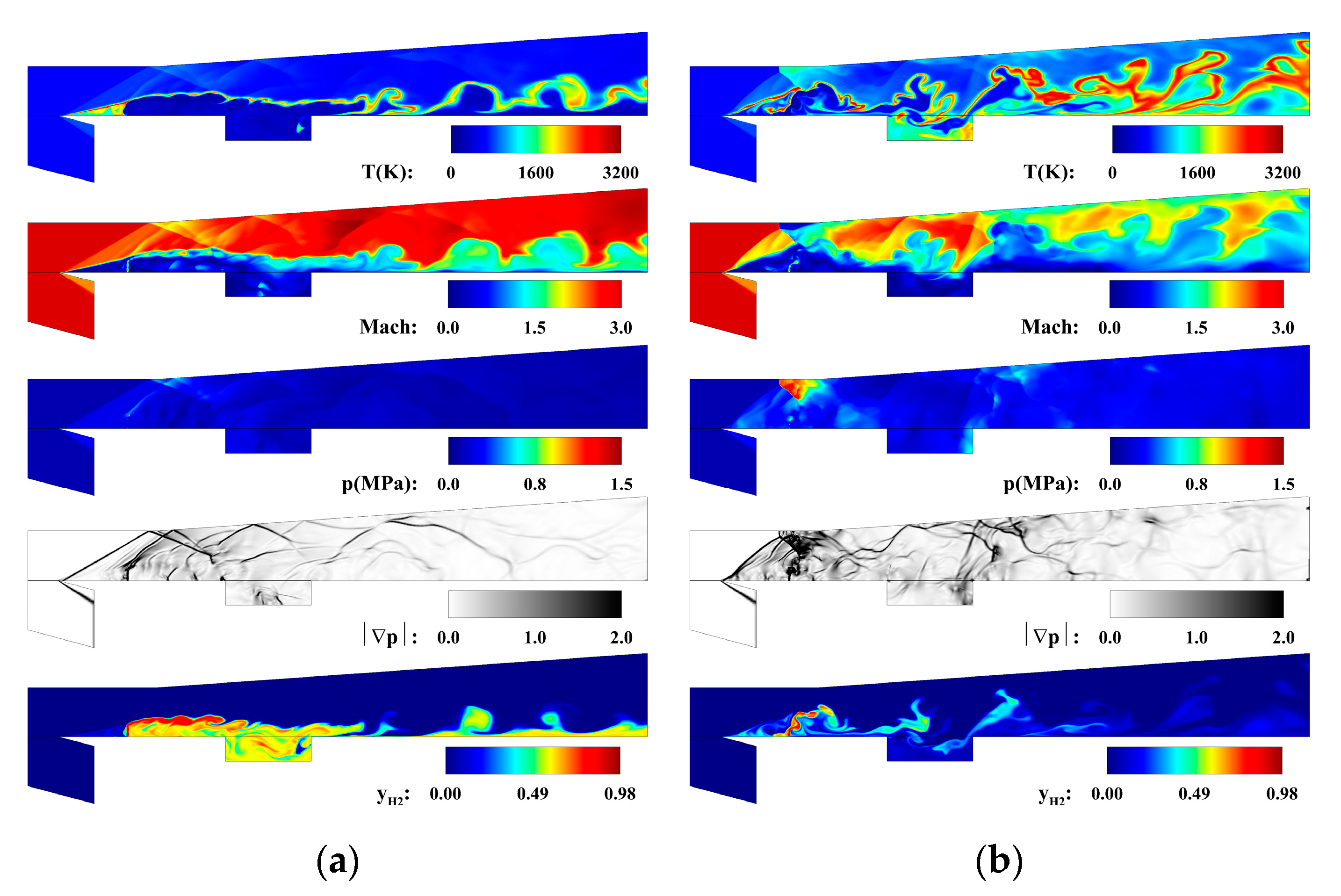
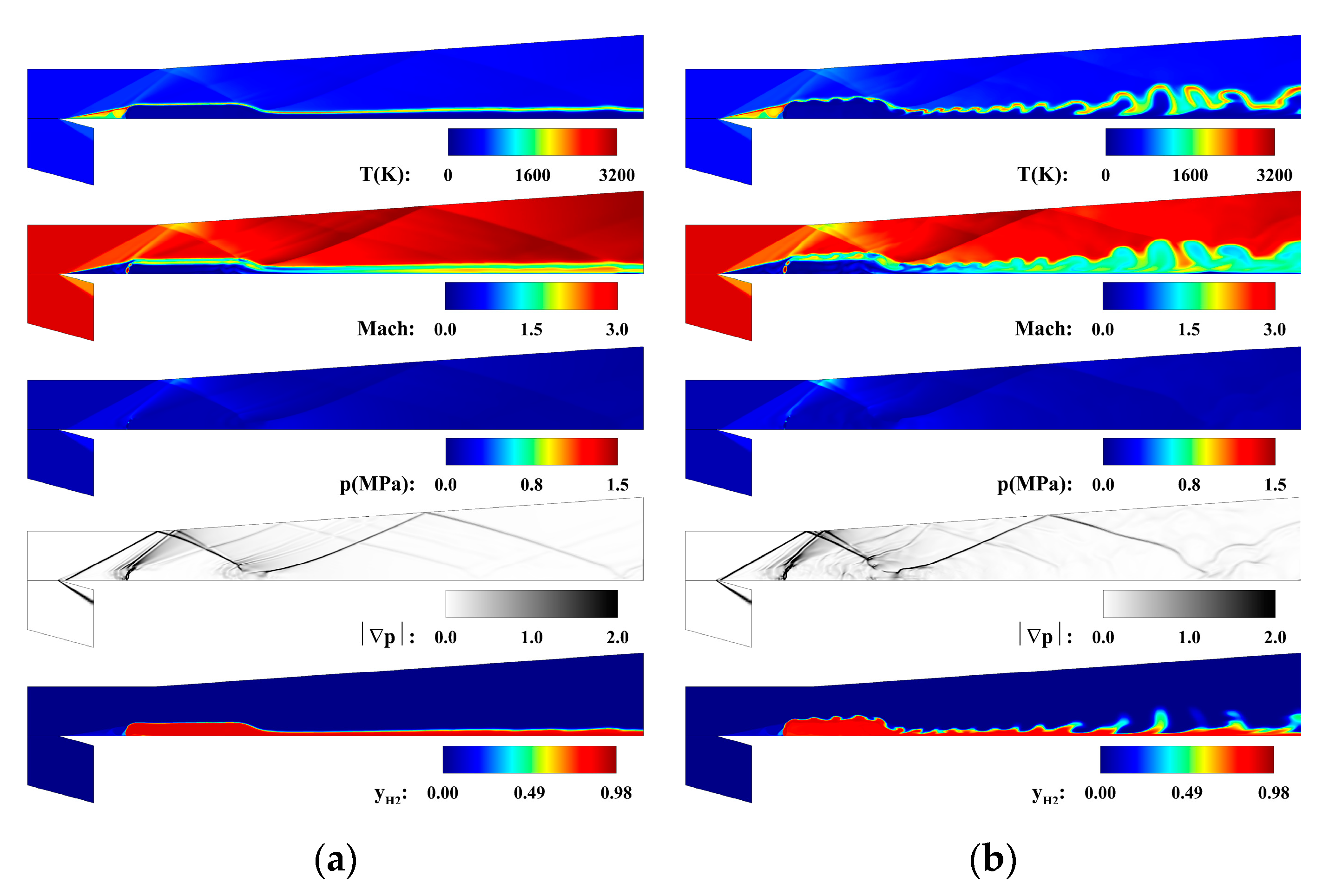
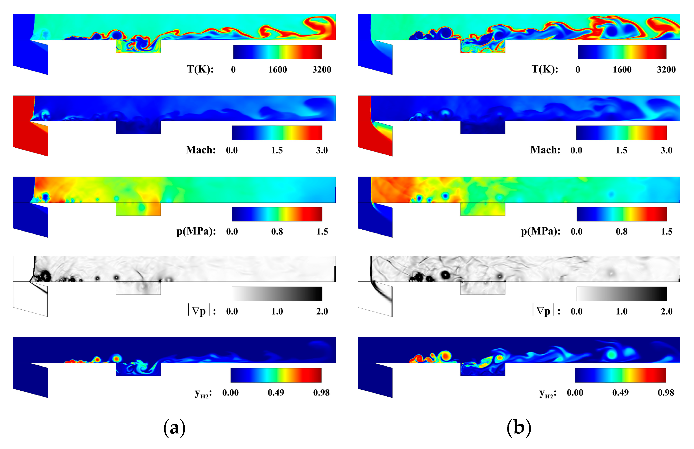
Twelve numerical experiment cases were conducted based on the combination of the three injection pressures, the presence of a cavity, and the two combustor shapes. However, because not all conditions exhibited different dynamic combustion characteristics, the results that produced the same results were omitted. Before describing the results of the combined diagnostic analysis, the numerical experiment is briefly discussed in this section. Six numerical experiments are illustrated in Figure 2, Figure 3 and Figure 4. All these Figures show the instantaneous results for the temperature, Mach number, pressure, pressure gradient, and fuel mass fraction fully developed at 30 ms, revealing the characteristics of the reacting flow in each combustor based on the injection pressures 0.75 MPa and 1.0 MPa.
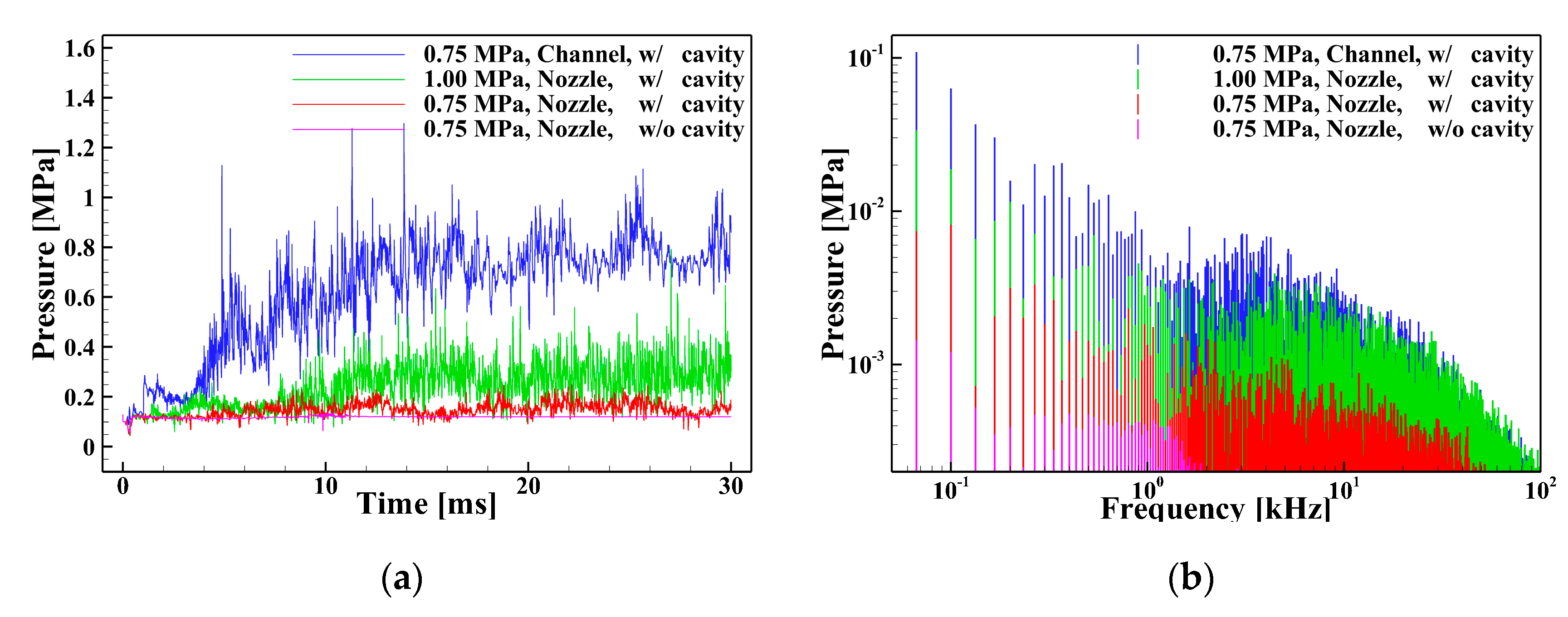
In Figure 2, as the injection pressure increased from 0.75 MPa to 1.0 MPa, the oblique shockwaves formed from the cowl lip were pulled to the front side of the inlet upper wall. Therefore, at the 1.0 MPa case, normal and oblique shockwaves are formed on the upper wall and induce strong pressure rise. In the 0.75 MPa injection pressure case, the injected fuel barely penetrated the main flow and flowed downstream along the bottom wall of the combustion chamber. However, in the 1.0 MPa injection pressure case, it can be observed that the injected fuel penetrated well into the main flow and strengthened the air–fuel mixing. This mixing characteristic can be verified by the fuel mass fraction contour that shows a high-mass fraction distribution at the injection site and cavity for the 0.75 MPa injection pressure case and immediate dissipation after injection for the 1.0 MPa injection pressure case. Figure 3 illustrates the instantaneous results for the diverging nozzle combustor without cavity and shows the importance of the cavity for fuel mixing. In the 0.75 MPa injection pressure case, it seems to be that the fuel penetrates to the main flow after injection. However, the fuel stream shows a tendency of stabilized combustion without disturbance. Then, the fuel stream flows downstream in a form attached to the lower wall by the influence of the reflected shockwave from the upper wall. The high temperature is distributed only in the region of the air–fuel mixing layer at the entire combustor. These characteristics of the reacting flow field at the 0.7 MPa case, clearly demonstrate the role of the cavity for fuel mixing and enhancing the combustion. At 1.0 MPa case, the fuel stream shows a fluctuation in the mixing layer immediately after injection. This motion becomes a large-scale fluctuation as the fuel stream goes downstream. This fluctuation enhances fuel mixing at downstream of the combustor, but it is not sufficient to compare this with a cavity case. In the case of the straight channel combustor, in both 0.75 MPa and 1.0 MPa cases, thermal choking occurred in the entire area of the combustor. A high-pressure distribution throughout the combustor formed by the thermal choking destroyed the shockwave structure in the inlet region, whereas the shockwave structure is still observed for the case of the diverging combustor. Due to the normal shockwaves formed in the inlet instead of oblique shocks, the Mach number of the main flow that comes through the intake was sharply reduced. This caused the increase in the residence time of the flow in the combustor to create an environment in which a chemical reaction could occur sufficiently. These combustors, which have been changed to subsonic combustion, not to supersonic combustion, showed significantly higher pressure and temperature distribution than the nozzle-type combustor due to the enhancing the combustion. Thermal choking and its effect can be better observed with the pressure history and FFT results shown in Figure 5. For the straight-channel combustor indicated as the blue line in Figure 5a, the pressure gradually increases over time, maintaining the levels of 0.6 MPa to 0.8 MPa. After 16 ms, when the thermal choking was estimated to be fully developed, the pressure fluctuates with constant periodicity. In contrast, the nozzle-type combustor tends to maintain the pressure at a certain level regardless of whether time after the reacting flow was fully developed in the combustor. However, there is a difference of more than 0.1 MPa in the pressure histories between the 0.75 MPa and 1.0 MPa injection pressure cases; thus, it can be clearly observed that the difference depends on the injection pressure. Additionally, the results plotted for the nozzle-type combustor without cavity show little pressure fluctuation during the entire time range, confirming the importance of the cavity for a supersonic combustor. In all FFT results shown in Figure 5b, the dominant frequencies are observed in the region below 1 kHz. Except for the case without the cavity, the major oscillation frequencies are distributed from 2 kHz~10 kHz, but high minor oscillation frequencies over 50 kHz are also detected. These major and minor oscillation frequencies distinguish the two combustor cases: the straight-channel combustor with an injection pressure of 0.75 MPa and the nozzle-type combustor with an injection pressure of 1.0 MPa. However, it is very difficult to ascertain whether minor oscillation frequency occurs during the process of pressure build-up or during the entire time range. Thus, it may be too soon to say that the dynamic characteristics of the pressure field have been identified through these analyses. To supplement the analyses, the dynamic combustion characteristics of this scramjet engine is analyzed using the diagnostic analysis methods presented in the subsequent sections.
3.2. Dynamic Characteristics of Frequency
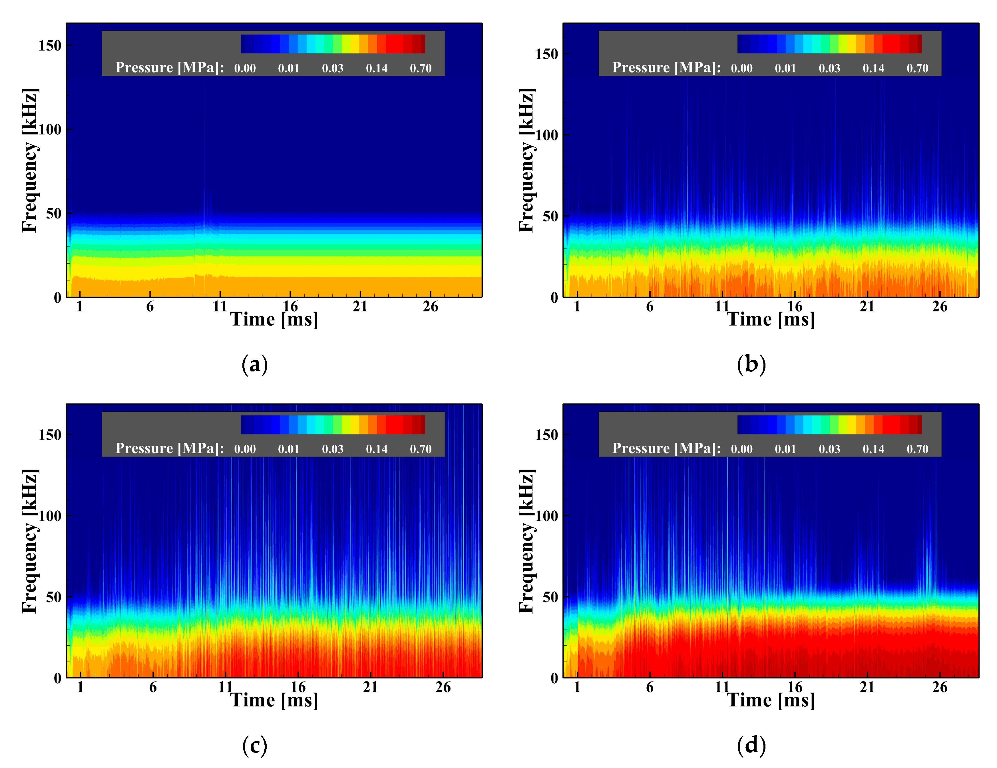
The STFT analysis was performed applying the Blackman–Harris window function and using the same data as that for the pressure history shown in Figure 5a. Because all four cases in Figure 6 have very different pressure ranges, the magnitude of pressure shown by color contour is represented in the log scale to maintain consistency in all cases.
The plot in Figure 6a is for the case with the nozzle-type combustor without cavity and shows poor air–fuel-mixing performance with a very consistent frequency throughout the entire time period except for some fluctuations in frequency detected at 9~10 ms. This result indicates that the stabilized combustion observed in Figure 3a shows the dominant characteristics for the entire time range. In contrast to the case without a cavity, when the cavity is present, a frequency oscillation of up to 100 kHz was detected with increasing unsteadiness of the flow field. These differences in the STFT results due to the presence of a cavity in 0.75 MPa injection pressure conditions were also predicted in the previous pressure history or FFT results in Figure 5b.
However, unlike the FFT analysis for the 0.75 MPa channel-type and 1.0 MPa nozzle-type cases, which included uncertainty in determining the dynamic characteristics of the frequency, the STFT analysis was able to clearly identify those characteristics. In the 1.0 MPa nozzle-type with a cavity case, illustrated in Figure 6c, the minor frequency oscillations above 50 kHz that were derived in the FFT results are evenly represented in the time region after 15 ms where the flow field is sufficiently developed. However, in the 0.75 MPa injection pressure straight-channel-type without a cavity case plotted in Figure 6d, these minor frequency oscillations are distributed evenly only within the time before 15 ms and occur with constant periodicity after 15 ms. These analysis results from the STFT indicate that the dynamic characteristics of the frequencies identified from the FFT results are not those corresponding to the entire time period.
3.3. Dynamic Characteristics of Propellant Mixing
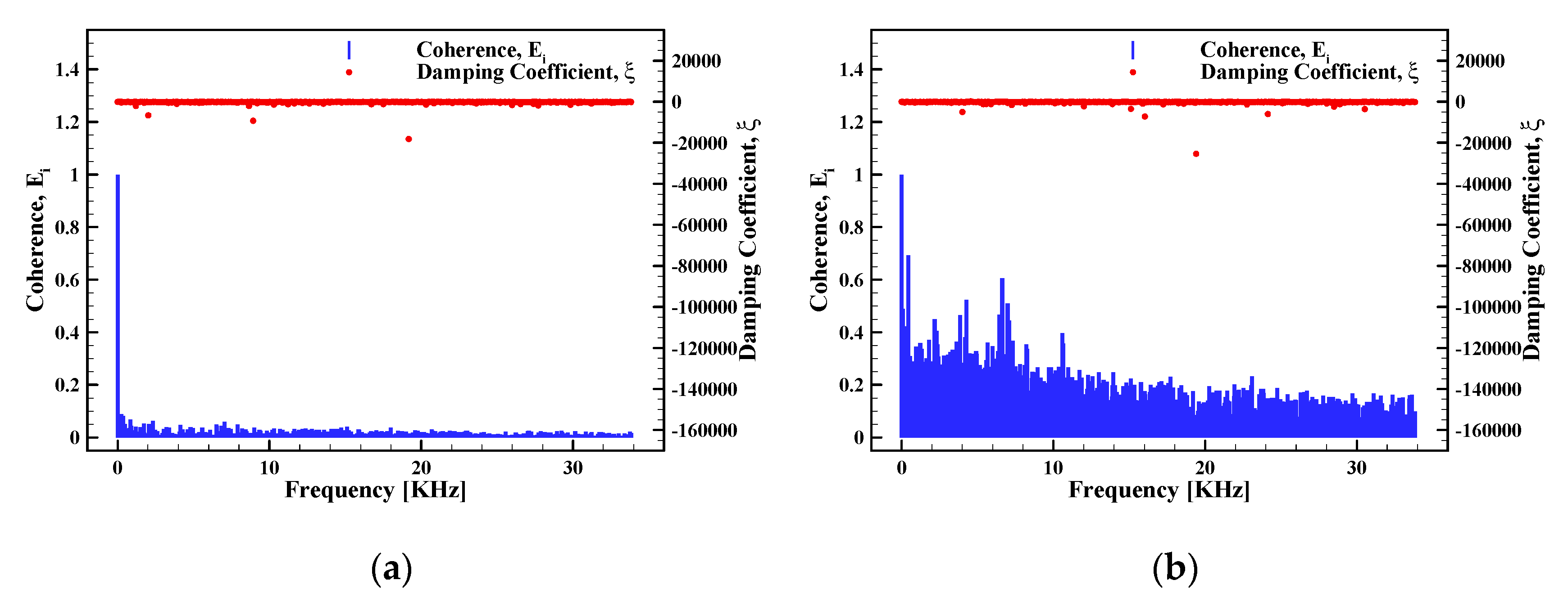
The DMD method can identify how the dynamic characteristics of propellant mixing, the most important issue in the scramjet engine, depend on the combustor shape and operating conditions. The results of two numerical experiment cases were analyzed: one with an injection pressure of 0.75 MPa and the other with 1.0 MPa but both using a nozzle-type combustor with a cavity. The spatial information of the H2 mass fraction, pressure, and pressure gradient of up to 30 ms physical time was used for the DMD analysis and over 1000 snapshots were applied. To maintain identical output time intervals between snapshots, the CFL (Courant–Friedrichs–Lewy condition) number was kept at 1.0 throughout the entire numerical experiment. A DMD analysis can derive the mode shape, frequency, damping coefficient, and coherence value of a system. Figure 7 illustrates the results of the DMD analysis for each condition. Here, the coherence value is an indicator of the relative energy between modes, which cannot be referred to as the absolute or quantitative energy of the mode but is capable of determining the energy ranking that each mode has. Among the derived DMD modes, the mode with the largest coherence value of 1.0 is called the mean mode. The mean mode is the spatial information that all snapshots belonging to the nonlinear system have. Therefore, the mean mode is very similar to the time-averaged data in the numerical experiment. In the present study, three modes with the largest values after the mean mode were selected and labeled as the 1st mode, 2nd mode, and 3rd mode. These modes, called sub-modes in the present work, dominate the dynamic characteristics of the flow field. Thus, to identify the dynamic characteristics using DMD, it is necessary to focus on all these sub-modes that contain the spatial information of the system dynamic changes represented as red and blue contours.
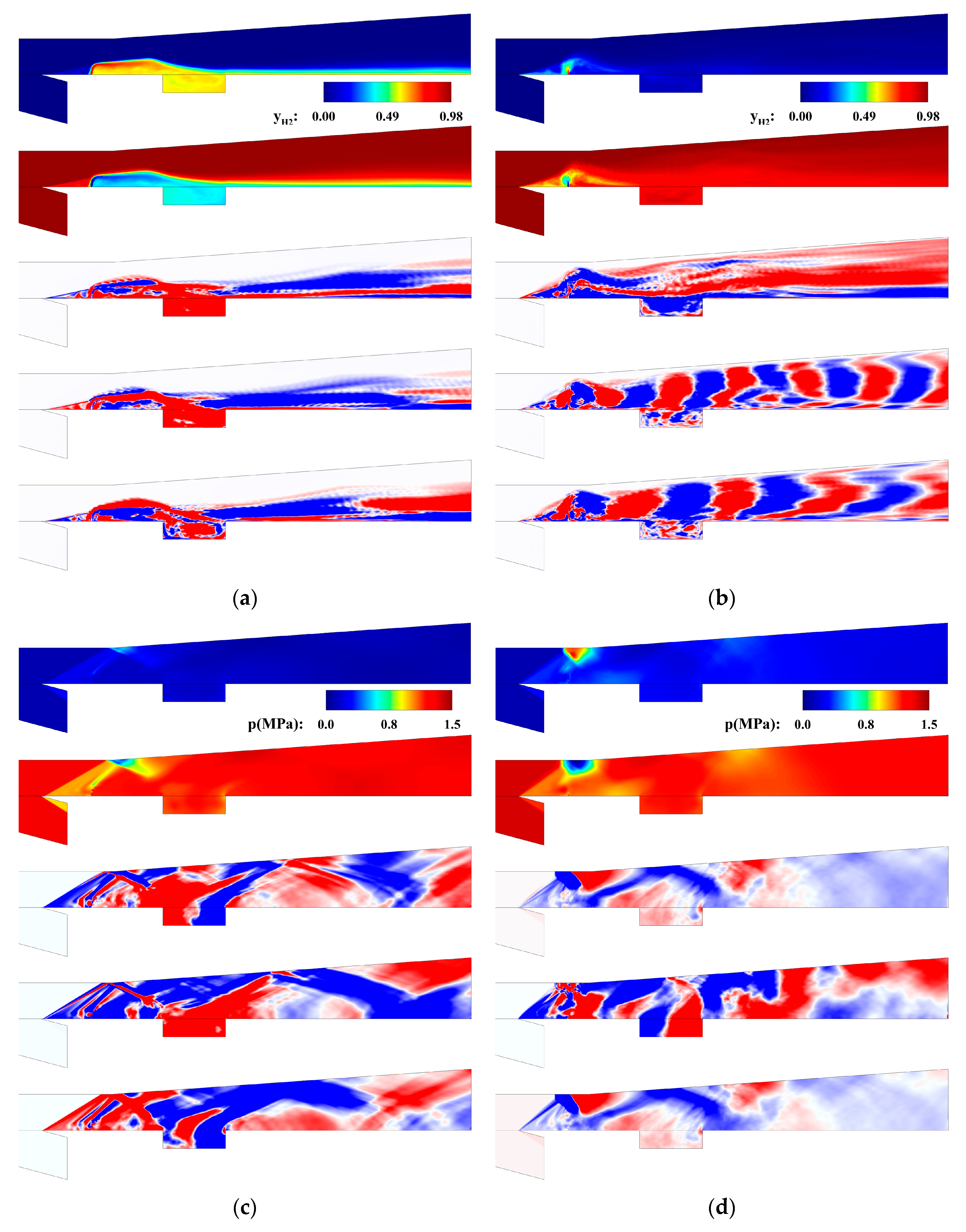
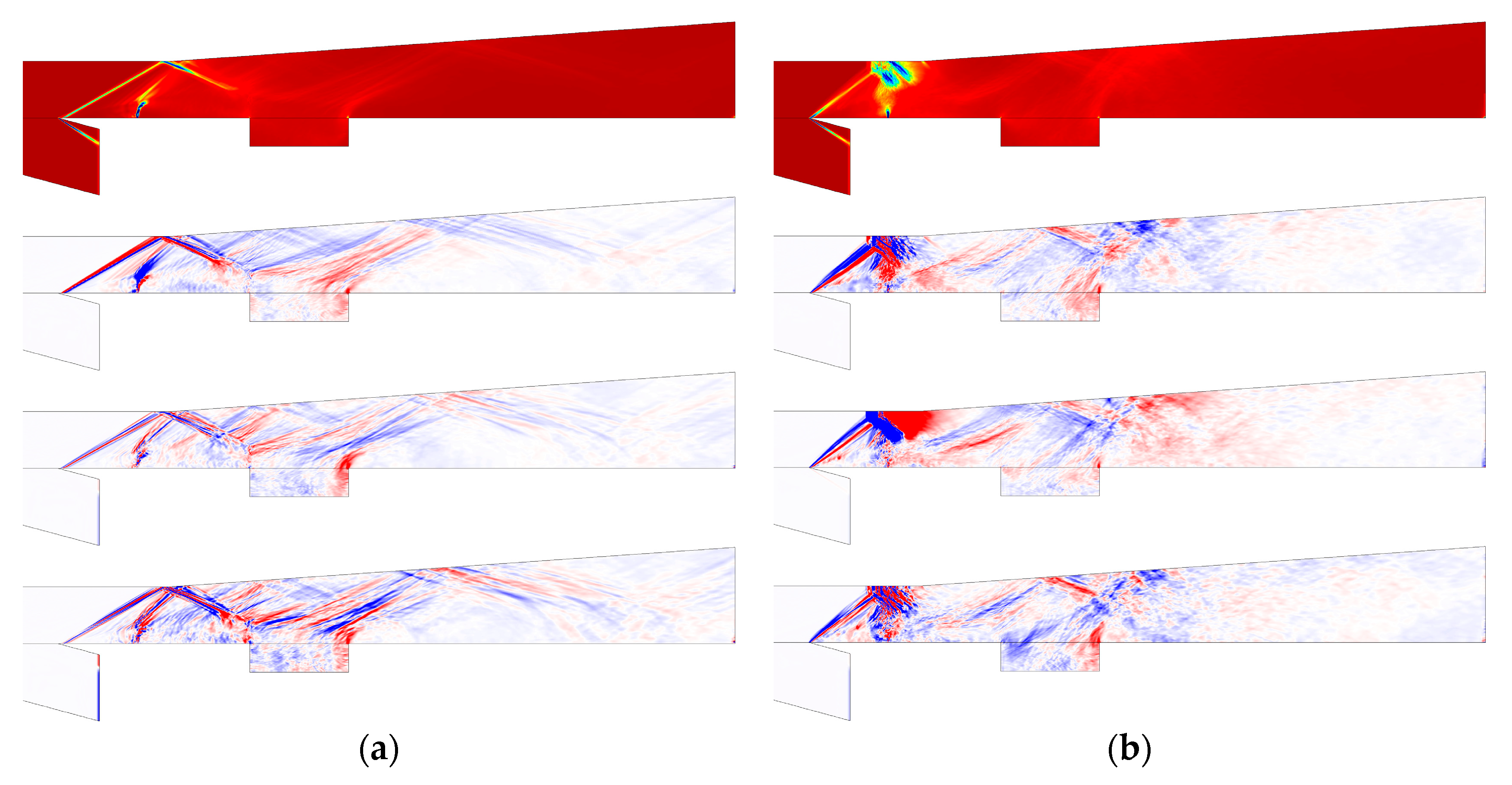
Figure 8 shows the time-averaged results and the DMD modes for the pressure and H2 mass fractions. Table 2 lists the frequency of each DMD mode. As mentioned previously, all the mean modes of the DMD results were derived similarly to the time-averaged results from the numerical experiments. Both the time-averaged results and the mean modes in Figure 8a show the behavior of the H2 mass fraction flowing downstream of the combustor without penetration into the main flow. The dynamic variation of the H2 mass fraction, which indicates the characteristics of air–fuel mixing, can be observed in the 1st, 2nd, and 3rd modes of Figure 8a. Here, in all the sub-modes, the H2 mass fraction has long intervals along the direction of the length of the combustor and exhibits fluctuations with a low-frequency range below 1 kHz. In the region after the cavity, it can be observed that the variations in the H2 mass fraction, which is divided into red and blue contours, are the same as the fluctuations of pressure shown in Figure 8c. Thus, it can be understood that this pressure fluctuation affects the fuel stream on the lower wall and triggers the propellant mixing in the longitudinal direction. In addition, this pressure variation is formed by an oblique shockwave of the cowl lip that is reflected between the upper and lower walls and progresses obliquely downstream of the combustor. The dynamic characteristics of these pressures appear to be the same in all sub-modes and demonstrate frequencies of up to 2 kHz or less.
The DMD results for the case with an injection pressure of 1.0 MPa show different dynamic characteristics, however. First, in the 2nd and 3rd modes in Figure 8c, the H2 mass fraction showed very short fluctuation intervals along the direction of the length of the combustor. These modes have frequencies that range from 4–6 kHz greater than 1 kHz, which is the frequency of the sub-modes for the case with the 0.75 MPa injection pressure. This implies that when the fuel is injected at 1.0 MPa, the time and spatial interval that dominate the propellant mixing performance will be considerably shorter than those in the previous conditions with 0.75 MPa injection pressure. In addition, the results of the 2nd and 3rd mode demonstrate that variations in the cavity and the main chamber is inhomogeneous, unlike the case with a 0.75 MPa injection pressure, which indicates that the variable regions at the injection point and in the cavity are same. These results indicate that under 1.0 MPa injection pressure conditions, the propellant mixing characteristics of the main combustor and those of the cavity are different from each other. The pressure results of the 1.0 MPa case illustrated in Figure 8d show different tendencies compared with the results of the 0.75 MPa case, particularly with the shock structure upstream and in the cavity. The oblique shockwave that started at the cowl lip meets the normal shockwave on the upper wall above the injection point. Then, a reflected shockwave is formed and interacts with the normal shockwave, generating a strong pressure gradient distribution in this region. During this process, it was found that the angle of the reflected wave that was formed by the oblique shockwave from the cowl lip grew larger as the injection pressure increased from 0.75 MPa to 1.0 MPa. The reflected shockwave reached the lower wall behind the injection point and progressed downstream of the combustor where it was reflected once more. This behavior is completely different from the case with the 0.75 MPa injection pressure in that the reflected wave progressed in the direction of the cavity, and this occurrence is observed for all the sub-modes of the case with a 1.0 MPa injection pressure. In addition, it can be observed that the pressure fluctuations in the cavity occur along the direction toward the top of the combustor and not in the oblique direction, which was the dominant mode shape for the case with the 0.75 MPa injection pressure. These results that demonstrate the different characteristics of propellant mixing and pressure distributions according to injection pressure suggest that there is a critical point at which the dynamic characteristics of this combustor completely changes between the injection pressures of 0.75 MPa and 1.0 MPa.
3.4. Dynamic Combustion Characteristics of a Scramjet Engine
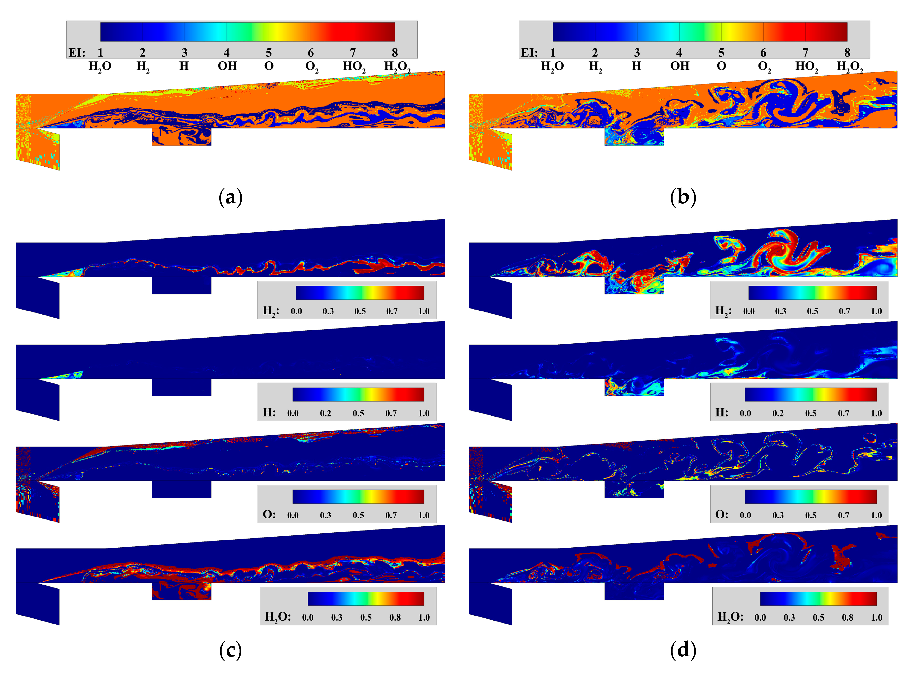
In the previous section, it was confirmed that the dynamic characteristics of the propellant mixing and pressure field in a combustor strongly depend on the injection pressure. In this section, CEMA is conducted to identify how these aspects change the flame structure and dynamic combustion characteristics. Figure 8 shows the dominant EI and normalized EI, which represent the contribution to the chemical explosive mode under the injection pressure conditions of 0.75 and 1.0 MPa. The CEMA results of the case with an injection pressure of 0.5 MPa were omitted because they were very similar to those of 0.75 MPa. All analyses, including the PI results to be described subsequently, used numerical analysis data at 30 ms. In Figure 9a or Figure 9c, which represent the EI results for the 0.75 MPa injection pressure case, it can be observed that H2 was involved in the chemical reaction only in the recirculation zone near the injection point and at the mixing layer of the fuel stream. Similarly, H is also detected only in the recirculation zone between the cowl lip and the injection point. Therefore, it can be confirmed that the recirculation and extinction of the fuel mass fraction in the cavity shown in the numerical analysis results do not lead to combustion, and only the recirculation region near the cowl lip governs the combustion reaction throughout the combustor. However, the EI results of the 1.0 MPa injection case in Figure 9b or Figure 9d demonstrate that H2 is found in all areas of the combustor, including the cavity, and, in particular, it is found that H is distributed inside the cavity. This indicates that the cavity, in which the flame holding and propellant mixing occur, is fully functional only under 1.0 MPa injection pressure conditions.
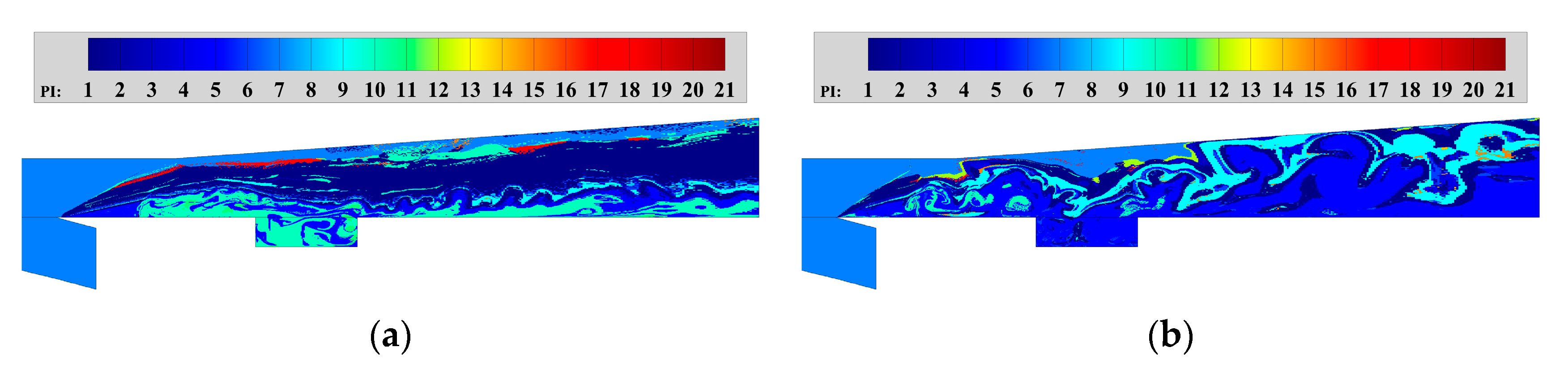
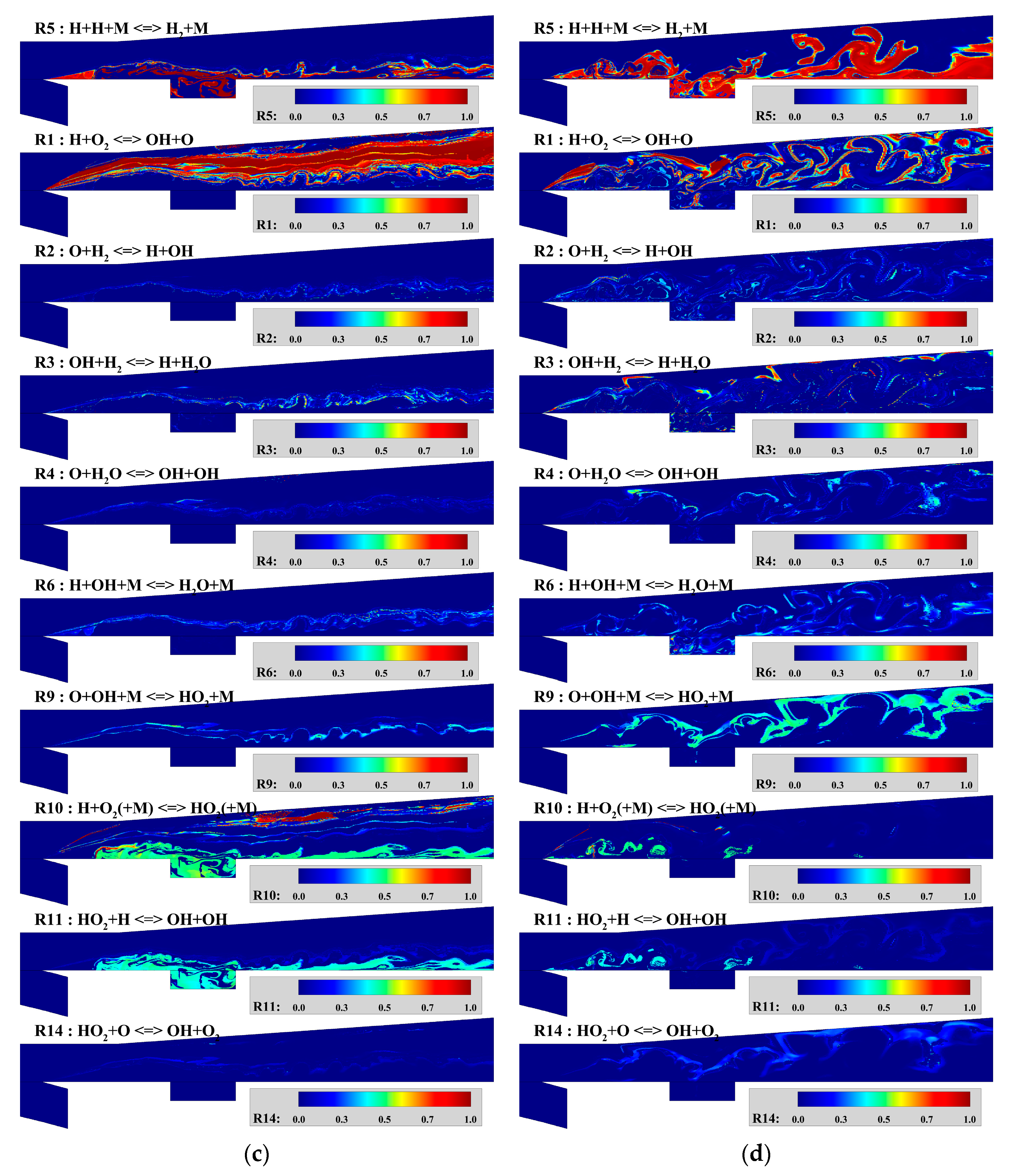
Before describing the PI results, it is important to note that PI is not calculated using an individual value of the forward and reverse reaction rate but rather by the net reaction rate. Therefore, each PI value does not represent a separate representation of the forward and reverse reactions. Furthermore, similar to the previous distribution of EI values, the dominant PI represents the strongest reaction step in the local area, and the normalized PI represents the spatial distribution for each reaction step. Figure 10 illustrates the dominant PI and the normalized PI. The figure for the normalized PI shows the steps that produce significantly different results based on each injection pressure, including the initial, chain-terminating, recombination steps. First, for the 0.75 MPa case in Figure 10a, it can be confirmed that the chain-reaction R1 was strongly detected in the main flow region. Also, it can be found that R10 and the initiation reaction R5 governed the injection point, cavity, and fuel stream. R1 and R5 were also identified in the 1.0 MPa case in Figure 10b, but the areas where they are located are very different. R5 was detected along the fuel stream distributed throughout the combustor after the injection, and R1 was detected only in the outer area of the mixed layer. Also, the R9 reaction, which is a three-body recombination reaction that includes the chain-terminating step involving O and OH radicals, was found inside the R1 region. But, the dominant reaction step R10, which was detected at the injection points and cavity under the 0.75 MPa condition, was weakly detected at the injection points in the case of 1.0 MPa. Even at the outermost layer of the main flow, slightly different distributions were identified for each injection pressure condition.
Figure 10c,d show the normalized PI by classifying the reaction steps of the UCSD hydrogen/oxygen chemical reaction mechanism as initiation, chain, chain-terminating reaction, and their reverse reactions. In the case of 0.75 MPa in Figure 10c, the fuel is injected and a strong R5 reaction occurs in the recirculation zone formed between the cowl lip and the injection point. However, after this region, the R5 reaction was captured only at the boundary of the fuel stream. As a result, the chain-reaction R1 reacted excessively along the mainstream, and the other chain-reaction reactions, R2, R3, and R4, occurred only in the areas where R5 was captured. The chain-terminating step R6 was also detected only around the region where the R5 reaction occurred. R9, one of the steps to activate R6, was shown to be distributed only in the outermost areas of the fuel stream. The R10 and R11 steps, which play the same role as R9, showed that they were over-distributed in areas containing the cavity and the injection point, and R14 demonstrated a very low level of reaction in the entire combustor. As with the previous dominant PI results, the normalized PI results of 1.0 MPa also showed a significantly different distribution for each reaction step. First, an R5 reaction was strongly detected throughout the combustor except at the upper wall above the injection point where the reflected shockwave formed. In this area, it was confirmed that any reactions including R5 did not take place due to the rapid pressure increase caused by the strong reflected shockwaves. Subsequently, R3, R2, R4, and R1 reactions occurred along the periphery of the R5 reaction region. These reactions were strongly detected inside the cavity, which shows that combustion took place actively inside the cavity in the 1.0 MPa case, unlike in the 0.75 MPa case. Moreover, the chain-terminating reaction R6 was detected in a similar region. The R9, R10, R11, and R14, to activate chain-terminating step R6, indicated different tendencies from those in the 0.75 MPa case. The R9 reaction showed a significantly stronger distribution than that in the 0.75 MPa case in the entire combustor region, whereas the R10 and R11 steps showed only weak reactions in the area near the injection point. All PI values for both combustor cases were different at all reaction steps. However, it is necessary to focus on certain reaction steps to determine the fundamental reason why each combustor had a different flame structure.
From the PI results of the two combustion conditions, the R1, R5, R10, and R11 reaction steps, which indicated the most significant differences, were thoroughly analyzed. Generally, in the case of hydrogen/oxygen chemical reactions, the initiation-reaction R5 is activated first, then the chain-reaction R1 reaction occurs, followed by the chain-terminating reaction R6. One of the reaction steps to complete the chain-terminating step R6 is the R10 step and, when this R10 step is activated, the R11 step is also activated sequentially. When the fuel mixing is adequate, this process, which would occur simultaneously, presented well under 1.0 MPa injection pressure conditions but not under 0.75 MPa conditions.
Close observation reveals that the results of the 0.75 MPa condition indicate two singular points. First, the H generated by the R5 reaction actively occurring in the recirculation region between the cowl lip and the injection point does not exhibit a spatial distribution that would sufficiently promote the chain reaction and, thus, the R1 reaction takes place away from the fuel stream. Second, the R10 reaction required to complete the chain-terminating step and the R11 reaction that occurs when the R10 reaction is activated are strongly distributed in the cavity region and behind the injection point. These singularities are also expected to be attributed to the dynamic characteristics of fuel mixing and the pressure indicated by the DMD analysis in the preceding section.
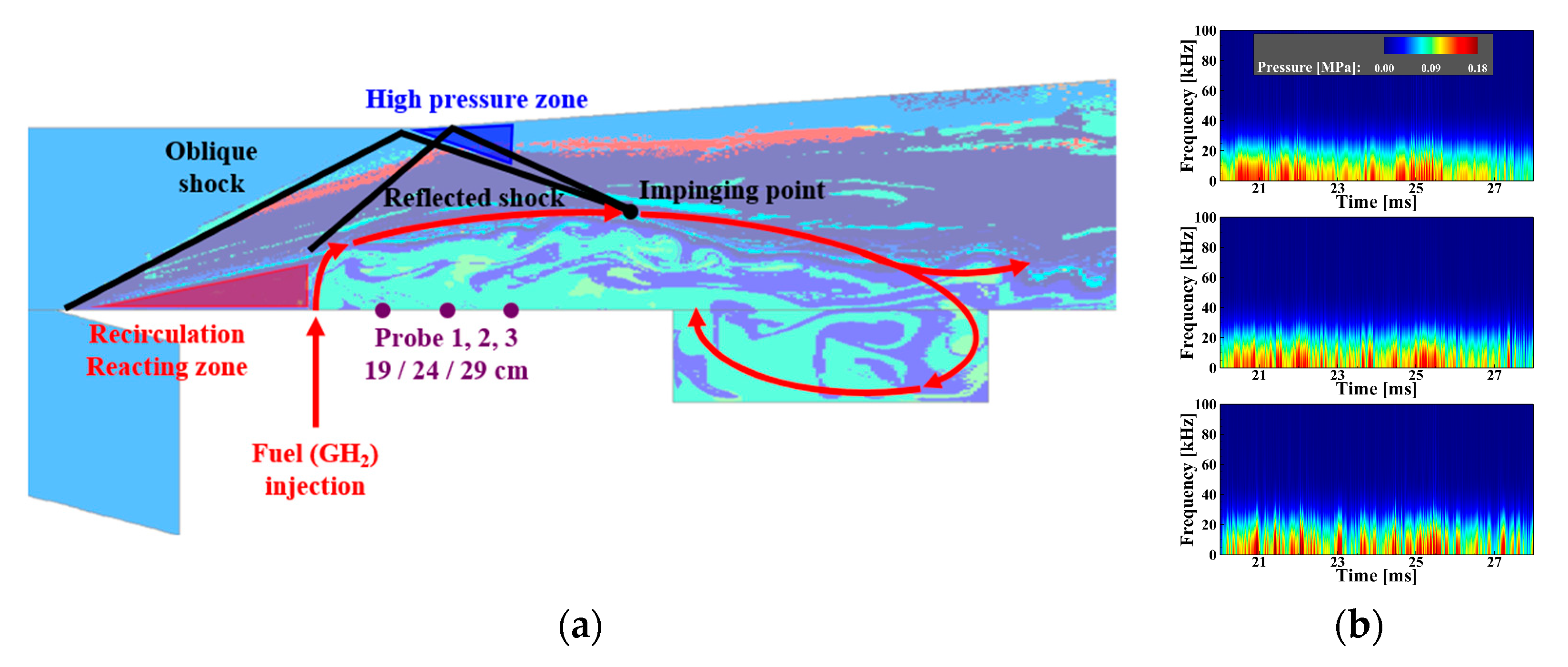
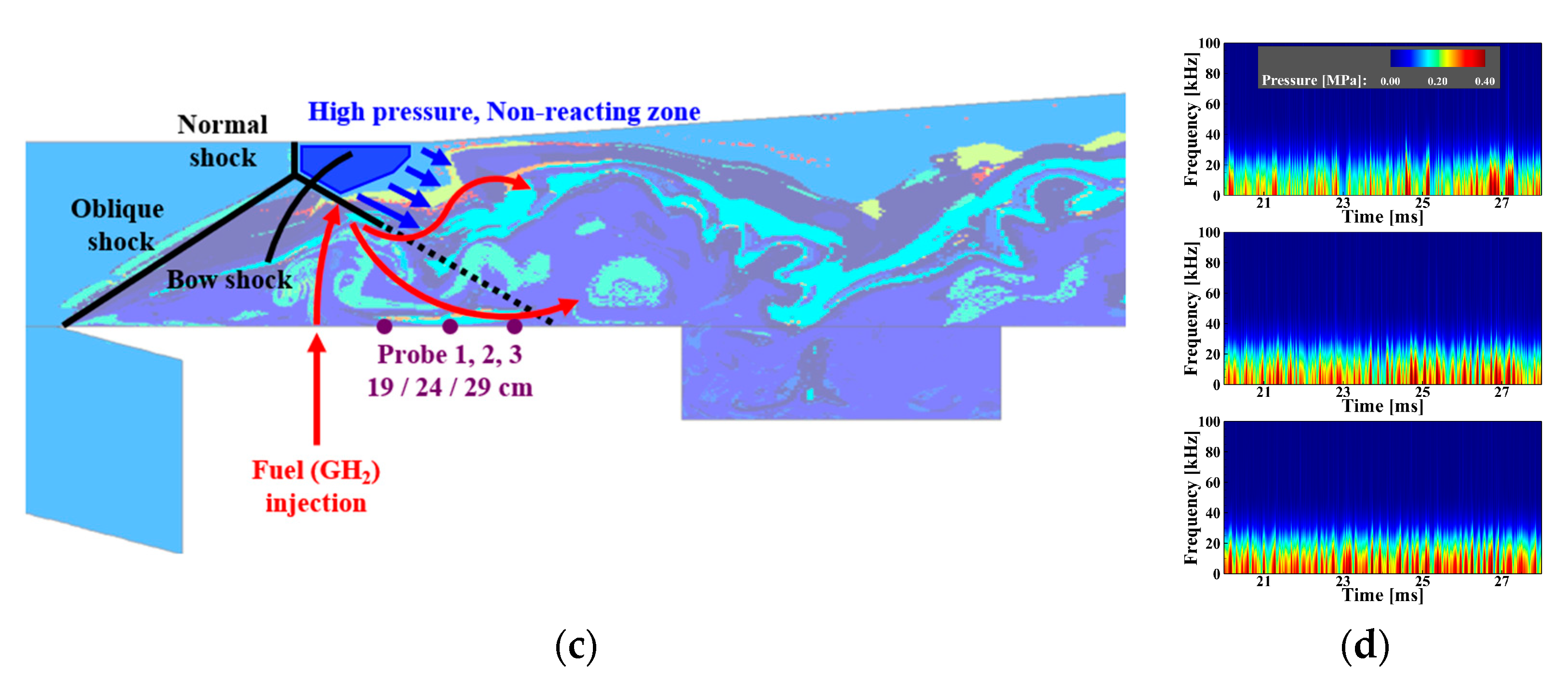
Figure 11 shows the behavior of the fuel stream for each combustor. For the 0.75 MPa condition shown in Figure 11a, two of the reflected shockwaves were generated on the upper wall by two oblique shockwaves formed from the cowl lip and the injection point. Additionally, the injected fuel did not sufficiently penetrate the mainstream and flows. The fuel stream that flowed toward the back wall of the cavity under the influence of strong pressure was caused by the merging of the two reflected shockwaves at the impinging point, as illustrated in the 1st and 3rd mode in Figure 12a. Thus, most fuel streams reach the cavity and form a recirculation zone. During this process of recirculation inside the cavity, some fuel streams return to the fuel injection point. The fuel stream that returned to the fuel injection point was recombined with the injected fuel and the above process repeated continuously. This process can also be observed in Figure 8a where the results of the DMD analysis for the H2 mass fraction are illustrated. The closed behavior of the fuel stream due to these reflected waves is considered a key factor in the dynamic combustion characteristics for conditions with a 0.75 MPa injection pressure. The case with a 1.0 MPa injection pressure in Figure 11c shows a completely different dynamic combustion characteristics. Oblique shockwaves formed on the cowl lip generated reflected waves with a much larger reflection angle than that in the 0.75 MPa case. A normal shockwave and a bow shockwave due to the fuel injection were also formed in the region of the upper wall where the reflected wave was formed, locally distributing a very strong pressure. Due to the high-pressure gradient, the injected fuel did not go to the upper wall area but flowed toward the lower wall or avoided this high-pressure area. For this reason, this high-pressure region locally exhibits a nonreacting flow. The flow direction of the fuel stream was reversed toward the upper wall after reaching the lower wall. After the cavity region, as the fuel stream alternated between the upper and lower walls, the fuel mixing was significantly enhanced compared with the case with a 0.75 MPa injection pressure, leading to an improved combustion performance. As a result, a spatially uniform pressure distribution was formed downstream of the combustor, as illustrated in Figure 12b. The behavior of the pressure field in the upstream region that determines the dynamic combustion characteristics of each scramjet engine can be validated by the STFT results for the three pressure measurement points shown in Figure 11b or Figure 11d. The STFT results for the 0.75 MPa injection pressure case demonstrates a high-pressure distribution with inconsistent time intervals at all measurement points. However, in the STFT results for the 1.0 MPa injection pressure case, it can be observed that the time interval at which a strong pressure is measured by probe 3, which was closest to the point where the fuel stream reaches the bottom wall, is the shortest. These results indicate that the difference in the pressure distribution based on the operating conditions of this combustor has a dominant effect on the fuel mixing and consequently is a key factor that determines the dynamic combustion characteristics.
4. Conclusions
To ascertain an approach and its effectiveness in identifying the dynamic combustion characteristics of a scramjet engine, a combined diagnostic analysis was conducted. The STFT, DMD, and CEMA were selected as the diagnostic analysis methods and two-dimensional numerical experiment data obtained from a scramjet engine similar to the Hyshot test model were utilized.
First, by using the STFT, the dynamic characteristics of frequency depending on the shape and operating conditions of each combustor were determined. Except for the case without a cavity, the major oscillations of less than 10 kHz and minor oscillations of greater than 50 kHz were detected in both the 0.75 MPa and 1.0 MPa injection pressure cases with the nozzle-type combustors. In contrast, in the channel-type combustor, only the major oscillations were detected as dominant with the minor oscillations occurring only intermittently after 16 ms when thermal choking was fully developed. The STFT was able to extract these characteristics clearly, a task that would have been difficult for the FFT. Next, under different injection pressure conditions, the spatial information of the fuel mass fraction and pressure was analyzed with DMD. The derived dynamic characteristics of the pressure distribution and propellant mixing were similar in both the 0.5 MPa and 0.75 MPa injection pressure cases but were completely different for the case with a 1.0 MPa injection pressure. Through this DMD analysis process, it was confirmed that a singular point exists between an injection pressure of 0.75 MPa and 1.0 MPa, at which the dynamic properties of this scramjet engine completely change. Lastly, based on the results from the STFT and DMD, a CEMA was performed to investigate the detailed flame structure and dynamic combustion characteristics of this scramjet engine. The CEMA results indicate that some of the reaction steps that generate the flame structure exhibit significantly different behaviors depending on the injection pressure. Additional analysis using the STFT and DMD revealed that these differences in the chemical reactions are governed by the structure of the different shockwaves upstream of the combustor formed under different injection pressure conditions. Therefore, the key factor in determining the dynamic combustion characteristics of this scramjet engine is the distribtion of the pressure field upstream of the combustor.
The diagnostic analysis methods used in this study are those that can be classified as postprocessing methods; therefore, these approaches inevitably depend on the results of numerical experiments and their accuracy. Nevertheless, this diagnostic analysis method is considered to be effective in identifying the dynamic combustion characteristics of a scramjet engine, as it can detect results that are challenging to distinguish in the data of a numerical experiment. In this study, it needed to maintain consistency with the previous numerical results to confirm the effectiveness of the combined diagnostic analysis methods. To satisfy this, a two-dimensional numerical analysis was performed. Therefore, for a more detailed combustion diagnostic analysis, three-dimensional numerical experiment must be performed. There are factors to keep in mind when performing DMD analysis. In the present work, the coherence value was used to select dominant DMD modes. This coherence value is relative energy between mean and sub-mode, not a quantity that can represent the absolute energy of each DMD mode. If the parameter that can represent the energy of each mode materialized, it is possible to derive more effective dynamic characteristics.
Author Contributions
Conceptualization, J.-Y.C.; methodology, S.-M.J.; investigation, S.-M.J.; writing—original draft preparation, S.-M.J.; writing—review and editing, J.-Y.C.; visualization, S.-M.J.; supervision, J.-Y.C.; project administration, J.-Y.C.; funding acquisition, J.-Y.C. All authors have read and agreed to the published version of the manuscript.
Funding
This research was funded by the Basic Research Program (No. 08-201-501-014) of the Agency for Defense Development (ADD) supported by the Defense Acquisition Program Administration (DAPA) of the Korean Government. Seung-Min Jeong was also funded by the NRF (National Research Foundation of Korea) granted by the Korean Government (NRF-2019-Global Ph.D. Fellowship Program).
Conflicts of Interest
The authors declare no conflict of interest.
References
- Choi, J.-Y.; Ma, F.; Yang, V. Dynamic Combustion Characteristics in Scramjet Combustors with Transverse Fuel Injection. AIAA Paper 2005-4428. In Proceedings of the 41st AIAA/ASME/SAE/ASEE Joint Propulsion Conference & Exhibit, Tucson, AZ, USA, 10–13 July 2005. [Google Scholar]
- Choi, J.-Y.; Ma, F.; Yang, V. Combustion oscillations in a scramjet engine combustor with transverse fuel injection. Proc. Combust. Inst. 2005, 30, 2851–2858. [Google Scholar] [CrossRef]
- Gerlinger, P.; Stoll, P.; Kindler, M.; Schneider, F.; Aigner, M. Numerical investigation of mixing and combustion enhancement in supersonic combustors by strut induced streamwise vorticity. Aerospace Sci. Technol. 2008, 12, 159–168. [Google Scholar] [CrossRef] [Green Version]
- Choi, J.; Noh, J.; Byun, J.-R.; Lim, J.-S.; Togai, K.; Yang, V. Numerical Investigation of Combustion/Shock-train Interactions in a Dual-Mode Scramjet Engine. AIAA Paper 2011-2395. In Proceedings of the 17th AIAA International Space Planes and Hypersonic Systems and Technologies Conference, San Francisco, CA, USA, 11–14 April 2011. [Google Scholar]
- Li, J.; Zhang, L.; Choi, J.; Yang, V.; Lin, K.-C. Ignition Transients in a Scramjet Engine with Air Throttling Part 1: Nonreacting Flow. J. Propuls. Power 2014, 30, 438–448. [Google Scholar] [CrossRef]
- Li, J.; Zhang, L.; Choi, J.Y.; Yang, V.; Lin, K.-C. Ignition Transients in a Scramjet Engine with Air Throttling Part II: Reacting Flow. J. Propuls. Power 2015, 31, 79–88. [Google Scholar] [CrossRef]
- Bermejo-Moreno, I.; Larsson, J.; Bodart, J.; Vicquelin, R. Wall-modeled large-eddy simulations of the HIFiRE-2 scramjet. Annu. Res. Briefs 2013, 2013, 3–19. [Google Scholar]
- Larsson, J.; Laurence, S.; Bermejo-Moreno, I.; Bodart, J.; Karl, S.; Vicquelin, R. Incipient thermal choking and stable shock-train formation in the heat-release region of a scramjet combustor. Part II: Large eddy simulations. Combust. Flame 2015, 162, 907–920. [Google Scholar] [CrossRef] [Green Version]
- Hwang, W.-S.; Seung-Min, J.; Choi, J. Fuel Temperature Effects on the Structure of Turbulent Supersonic Combustion at Constant Mass Flow Condition. AIAA Paper 2017-4944. In Proceedings of the 53rd AIAA/SAE/ASEE Joint Propulsion Conference, Atlanta, GA, USA, 10–12 July 2017. [Google Scholar]
- Liu, C.; Wang, Z.; Wang, H.; Sun, M.; Li, P. Large eddy simulation of cavity-stabilized hydrogen combustion in a diverging supersonic combustor. Int. J. Hidrog. Energy 2017, 42, 28918–28931. [Google Scholar] [CrossRef]
- Moradi, R.; Mahyari, A.; Barzegar Gerdroodbary, M.; Abdollahi, A.; Amini, Y. Shape effect of cavity flameholder on mixing zone of hydrogen jet at supersonic flow. Int. J. Hidrog. Energy 2018, 43, 16364–16372. [Google Scholar] [CrossRef]
- Edalatpour, A.; Hassanvand, A.; Gerdroodbary, M.B.; Moradi, R.; Amini, Y. Injection of multi hydrogen jets within cavity flameholder at supersonic flow. Int. J. Hidrog. Energy 2019, 44, 13923–13931. [Google Scholar] [CrossRef]
- Griffin, D.; Lim, J. Signal estimation from modified short-time Fourier transform. IEEE Trans. Acoustics Speech Signal Process. 1984, 32, 236–243. [Google Scholar] [CrossRef]
- Schmid, P.J. Dynamic mode decomposition of numerical and experimental data. J. Fluid Mech. 2010, 656, 5–28. [Google Scholar] [CrossRef] [Green Version]
- Taira, K.; Brunton, S.L.; Dawson, S.T.; Rowley, C.W.; Colonius, T.; McKeon, B.J.; Schmidt, O.T.; Gordeyev, S.; Theofilis, V.; Ukeiley, L.S. Modal analysis of fluid flows: An overview. AIAA J. 2017, 55, 4013–4041. [Google Scholar] [CrossRef] [Green Version]
- Jeong, S.-M. Analysis for Characteristic of Turbulent Combustion and Combustion Instability of Gaseous Hydrogen/Gaseous Oxygen Rocket Combustor Using Dynamic Mode Decomposition. Master’s Thesis, Pusan National University, Busan, Korea, 29 June 2018. [Google Scholar]
- Pavalavanni, P.K.; Sohn, C.H.; Lee, B.J.; Choi, J.-Y. Revisiting unsteady shock-induced combustion with modern analysis techniques. Proc. Combust. Inst. 2019, 37, 3637–3644. [Google Scholar] [CrossRef]
- Lu, T.; Yoo, C.; Chen, J.; Law, C. Analysis of a turbulent lifted hydrogen/air jet flame from direct numerical simulation with computational singular perturbation. AIAA Paper 2008-1013. In Proceedings of the 46th AIAA Aerospace Sciences Meeting and Exhibit, Reno, NV, USA, 7–10 January 2008. [Google Scholar]
- Lu, T.; Yoo, C.S.; Chen, J.; Law, C.K. Three-dimensional direct numerical simulation of a turbulent lifted hydrogen jet flame in heated coflow: A chemical explosive mode analysis. J. Fluid Mech. 2010, 652, 45–64. [Google Scholar] [CrossRef]
- Smart, M.K.; Hass, N.E.; Paull, A. Flight Data Analysis of the HyShot 2 Scramjet Flight Experiment. AIAA J. 2006, 44, 2366–2375. [Google Scholar] [CrossRef]
- Hinterberger, C.; Fröhlich, J.; Rodi, W. Three-Dimensional and Depth-Averaged Large-Eddy Simulations of Some Shallow Water Flows. J. Hydraul. Eng. 2007, 133, 857–872. [Google Scholar] [CrossRef]
- Wada, Y.; Liou, M.-S. An accurate and robust flux splitting scheme for shock and contact discontinuities. SIAM J. Sci. Comput. 1997, 18, 633–657. [Google Scholar] [CrossRef]
- Gritskevich, M.S.; Garbaruk, A.V.; Schütze, J.; Menter, F.R. Development of DDES and IDDES Formulations for the k-ω Shear Stress Transport Model. Flow Turbul. Combust. 2012, 88, 431–449. [Google Scholar] [CrossRef]
- The San Diego Mechanism. Available online: https://web.eng.ucsd.edu/mae/groups/combustion/mechanism.html (accessed on 26 February 2014).
- Kumar, P.P.; Kim, K.-S.; Oh, S.; Choi, J.-Y. Numerical comparison of hydrogen-air reaction mechanisms for unsteady shock-induced combustion applications. J. Mech. Sci. Technol. 2015, 29, 893–898. [Google Scholar] [CrossRef]
- Torregrosa, A.J.; Broatch, A.; García-Tíscar, J.; Gomez-Soriano, J. Modal decomposition of the unsteady flow field in compression-ignited combustion chambers. Combust. Flame 2018, 188, 469–482. [Google Scholar] [CrossRef]
Figure 1.
Configuration of a scramjet engine from previous numerical experiment performed by Choi et al. [1]
Figure 1.
Configuration of a scramjet engine from previous numerical experiment performed by Choi et al. [1]

Figure 2.
Instantaneous result for diverging nozzle combustor with cavity based on the injection pressures: (a) 0.75 MPa and (b) 1.00 MPa.
Figure 2.
Instantaneous result for diverging nozzle combustor with cavity based on the injection pressures: (a) 0.75 MPa and (b) 1.00 MPa.

Figure 3.
Instantaneous result for diverging nozzle combustor without cavity based on the injection pressures: (a) 0.75 MPa and (b) 1.00 MPa.
Figure 3.
Instantaneous result for diverging nozzle combustor without cavity based on the injection pressures: (a) 0.75 MPa and (b) 1.00 MPa.

Figure 4.
Instantaneous result for straight-channel combustor with cavity based on the injection pressures: (a) 0.75 MPa and (b) 1.00 MPa.
Figure 4.
Instantaneous result for straight-channel combustor with cavity based on the injection pressures: (a) 0.75 MPa and (b) 1.00 MPa.

Figure 5.
Results for a point at 59 cm on the lower wall surface: (a) pressure history and (b) FFT results for pressure history.
Figure 5.
Results for a point at 59 cm on the lower wall surface: (a) pressure history and (b) FFT results for pressure history.

Figure 6.
The STFT results for the pressure history of each case: (a) 0.75 MPa, nozzle-type, w/o cavity; (b) 0.75 MPa, nozzle-type, w/cavity; (c) 1.0 MPa, nozzle-type, w/cavity; (d) 0.75 MPa, straight-channel-type, w/o cavity.
Figure 6.
The STFT results for the pressure history of each case: (a) 0.75 MPa, nozzle-type, w/o cavity; (b) 0.75 MPa, nozzle-type, w/cavity; (c) 1.0 MPa, nozzle-type, w/cavity; (d) 0.75 MPa, straight-channel-type, w/o cavity.

Figure 7.
Mode frequency, damping coefficient, and coherence value derived from the DMD analysis for the H2 mass fraction: (a) 0.75 MPa and (b) 1.00 MPa injection pressure condition.
Figure 7.
Mode frequency, damping coefficient, and coherence value derived from the DMD analysis for the H2 mass fraction: (a) 0.75 MPa and (b) 1.00 MPa injection pressure condition.

Figure 8.
(In order from top to bottom) time-averaged results of the numerical experiments, mean mode, 1st mode, 2nd mode, 3rd mode of the DMD: H2 mass fraction at (a) 0.75 MPa and (b) 1.00 MPa; pressure distribution at (c) 0.75 MPa and (d) 1.0 MPa.
Figure 8.
(In order from top to bottom) time-averaged results of the numerical experiments, mean mode, 1st mode, 2nd mode, 3rd mode of the DMD: H2 mass fraction at (a) 0.75 MPa and (b) 1.00 MPa; pressure distribution at (c) 0.75 MPa and (d) 1.0 MPa.

Figure 9.
Results of the chemical mode explosive analysis for each injection pressure case: dominant EI results for (a) 0.75 MPa and (b) 1.0 MPa; normalized EI results for (c) 0.75 MPa and (d) 1.0 MPa.
Figure 9.
Results of the chemical mode explosive analysis for each injection pressure case: dominant EI results for (a) 0.75 MPa and (b) 1.0 MPa; normalized EI results for (c) 0.75 MPa and (d) 1.0 MPa.

Figure 10.
Results of the chemical mode explosive analysis for each injection pressure case: dominant PI results for (a) 0.75 MPa and (b) 1.0 MPa; normalized PI results for (c) 0.75 MPa and (d) 1.0 MPa.
Figure 10.
Results of the chemical mode explosive analysis for each injection pressure case: dominant PI results for (a) 0.75 MPa and (b) 1.0 MPa; normalized PI results for (c) 0.75 MPa and (d) 1.0 MPa.


Figure 11.
Schematic diagram of the reacting flow field and the STFT results for pressure at probe points 1, 2, and 3: (a), (b) 0.75 MPa; (c), (d) 1.0 MPa injection pressure condition.
Figure 11.
Schematic diagram of the reacting flow field and the STFT results for pressure at probe points 1, 2, and 3: (a), (b) 0.75 MPa; (c), (d) 1.0 MPa injection pressure condition.


Figure 12.
(In order from top to bottom) mean mode, 1st mode, 2nd mode, and 3rd mode of the DMD analysis: pressure gradient at (a) 0.75 MPa and (b) 1.00 MPa injection pressure.
Figure 12.
(In order from top to bottom) mean mode, 1st mode, 2nd mode, and 3rd mode of the DMD analysis: pressure gradient at (a) 0.75 MPa and (b) 1.00 MPa injection pressure.


Table 1.
Hydrogen/air pressure-dependent reaction mechanism introduced by UC San Diego [24].
Table 1.
Hydrogen/air pressure-dependent reaction mechanism introduced by UC San Diego [24].
| No. | Reaction | A | n | EA |
|---|---|---|---|---|
| R1 | H+O2 ↔ OH+O | 3.52 × 10¹⁶ | −0.70 | 17,069 |
| R2 | O+H2 ↔ H+OH | 5.06 × 10⁴ | 2.67 | 6290.63 |
| R3 | OH+H2 ↔ H+H2O | 1.17 × 10⁹ | 1.30 | 3635.28 |
| R4 | O+H2O ↔ OH+OH | 7.00 × 10⁵ | 2.33 | 14,548.28 |
| R5 | H+H+M ↔ H2+M | 1.30 × 10¹⁸ | −1.00 | 0 |
| R6 | H+OH+M ↔ H2O+M | 4.00 × 10²² | −2.00 | 0 |
| R7 | O+O+M ↔ O2+M | 6.17 × 10¹⁵ | −0.50 | 0 |
| R8 | H+O+M ↔ OH+M | 4.71 × 10¹⁸ | −1.00 | 0 |
| R9 | O+OH+M ↔ HO2+M | 8.00 × 10¹⁵ | 0.00 | 0 |
| R10 | H+O2(+M)↔HO2(+M) | |||
| High Pressure | 4.65 × 10¹² | 0.44 | 0 | |
| Low Pressure | 5.75 × 10¹⁹ | −1.40 | 0 | |
| Troe form | ||||
| R11 | HO2+H ↔ OH+OH | 7.08 × 10¹³ | 0.00 | 0 |
| R12 | HO2+H ↔ H2+O2 | 1.66 × 10¹³ | 0.00 | 0 |
| R13 | HO2+H ↔ H2O+O | 3.10 × 10¹³ | 0.00 | 0 |
| R14 | HO2+O ↔ OH+O2 | 2.00 × 10¹³ | 0.00 | 0 |
| R15 | HO2+OH ↔ H2O+O2 | 7.00 × 10¹² | 0.00 | 0 |
| Duplicate | 4.50 × 10¹⁴ | 0.00 | 0 | |
| R16 | OH+OH(+M)↔H2O2(+M) | |||
| High Pressure | 9.55 × 10¹³ | −0.27 | 0 | |
| Low Pressure | 2.76 × 1025 | −3.20 | 0 | |
| Troe form | ||||
| R17 | HO2+HO2↔ H2O2+O2 | 1.03 × 10¹⁴ | 0.00 | 11,042.07 |
| Duplicate | 1.94 × 10¹¹ | 0.00 | −1408.94 | |
| R18 | H2O2+H ↔ HO2+H2 | 2.30 × 10¹³ | 0.00 | 7950.05 |
| R19 | H2O2+H ↔ OH+H2O | 1.00 × 10¹³ | 0.00 | 3585.09 |
| R20 | H2O2+OH ↔ HO2+H2O | 1.74 × 10¹² | 0.00 | 1434.03 |
| Duplicate | 7.59 × 10¹³ | 0.00 | 7272.94 | |
| R21 | H2O2+O ↔ HO2+OH | 9.63 × 10⁶ | 2.00 | 3991.40 |
| Third body efficiencies relative to N2 | ||||
| R5 | H+H+M ↔ H2+M | H2 = 1.5 | H2O = 11.0 | |
| R6 | H+OH+M ↔ H2O+M | H2 = 1.5 | H2O = 11.0 | |
| R7 | O+O+M ↔ O2+M | H2 = 1.5 | H2O = 11.0 | |
| R8 | H+O+M ↔ OH+M | H2 = 1.5 | H2O = 11.0 | |
| R9 | O+OH+M ↔ HO2+M | H2 = 1.5 | H2O = 11.0 | |
| R10 | H+O2(+M) ↔ HO2(+M) | H2 = 1.5 | H2O = 15.0 | |
| R16 | OH+OH(+M) ↔ H2O2(+M) | H2 = 1.0 | H2O = 5.0 | |
, , : coefficient of Treo form, Fcent = −(1−)Exp(−T/ T***) +Exp(−T/T*).
Table 2.
Frequencies of all DMD modes according to injection pressure.
| Mode | 0.75 MPa Case | 1.0 MPa Case |
|---|---|---|
| Mean mode | 0.00 kHz 1/0.00 kHz 2 | 0.00 kHz 1/0.00 kHz 2 |
| 1st mode | 0.24 kHz 1/1.93 kHz 2 | 0.44 kHz 1/0.09 kHz 2 |
| 2nd mode | 0.35 kHz 1/1.15 kHz 2 | 6.63 kHz 1/2.26 kHz 2 |
| 3rd mode | 0.84 kHz 1/1.41 kHz 2 | 4.27 kHz 1/0.15 kHz 2 |
Frequency information of 1 H2 mass fraction/2 pressure.
© 2020 by the authors. Licensee MDPI, Basel, Switzerland. This article is an open access article distributed under the terms and conditions of the Creative Commons Attribution (CC BY) license (http://creativecommons.org/licenses/by/4.0/).
Share and Cite
MDPI and ACS Style
Jeong, S.-M.; Choi, J.-Y. Combined Diagnostic Analysis of Dynamic Combustion Characteristics in a Scramjet Engine. Energies 2020, 13, 4029. https://doi.org/10.3390/en13154029
AMA Style
Jeong S-M, Choi J-Y. Combined Diagnostic Analysis of Dynamic Combustion Characteristics in a Scramjet Engine. Energies. 2020; 13(15):4029. https://doi.org/10.3390/en13154029
Chicago/Turabian StyleJeong, Seung-Min, and Jeong-Yeol Choi. 2020. "Combined Diagnostic Analysis of Dynamic Combustion Characteristics in a Scramjet Engine" Energies 13, no. 15: 4029. https://doi.org/10.3390/en13154029
Note that from the first issue of 2016, this journal uses article numbers instead of page numbers. See further details here.