Microgrid Fault Detection and Classification: Machine Learning Based Approach, Comparison, and Reviews

Abstract

Accurate fault classification and detection for the microgrid (MG) becomes a concern among the researchers from the state-of-art of fault diagnosis as it increases the chance to increase the transient response. The MG frequently experiences a number of shunt faults during the distribution of power from the generation end to user premises, which affects the system reliability, damages the load, and increases the fault line restoration cost. Therefore, a noise-immune and precise fault diagnosis model is required to perform the fast recovery of the unhealthy phases. This paper presents a review on the MG fault diagnosis techniques with their limitations and proposes a novel discrete-wavelet transform (DWT) based probabilistic generative model to explore the precise solution for fault diagnosis of MG. The proposed model is made of multiple layers with a restricted Boltzmann machine (RBM), which enables the model to make the probability reconstruction over its inputs. The individual RBM layer is trained with an unsupervised learning approach where an artificial neural network (ANN) algorithm tunes the model for minimizing the error between the true and predicted class. The effectiveness of the proposed model is studied by varying the input signal and sampling frequencies. A level of considered noise is added with the sample data to test the robustness of the studied model. Results prove that the proposed fault detection and classification model has the ability to perform the precise diagnosis of MG faults. A comparative study among the proposed, kernel extreme learning machine (KELM), multi KELM, and support vector machine (SVM) approaches is studied to confirm the robust superior performance of the proposed model.

1. Introduction

The microgrid (MG) meets the exponential growth of load demand because of its reliable, secure, sustainable, and green energy supply [1,2]. This small-scale power supply network is constituted by several distributed energy resources (DERs), energy storage devices, communication facilities, and well-regulated loads [3,4,5]. An MG is able to work in both an autonomous/islanded and grid-tied way. In the grid-tied operation, a portion of the load is driven by the primary AC grid, and in the islanded process, the main AC grid is disconnected from the microgrid and runs autonomously. As the MG shows dynamic (such as the mode of operation) characteristics and its system components show non-linear characteristics, it produces a negative influence on the system protection [6]. Thus, the protection of the MG system is a considerable issue before facilitating this novel technology [7,8,9,10,11].

The safe operation of the MG depends on the precise fault detection and classification (FDC) as the faults are unpredictable and random in nature and needs specialized technique to restore the faulty phases [12,13]. Furthermore, the protection method of the MG is not directly comparable to the conventional transmission line protection method due to its various modes of operation (autonomous or grid-tied), system arrangement (looped or radial), and types of DERs. An amount of short circuit faults like phase-to-phase (pp), phase-to-ground (PG), two PG (2PG), and three PG (3PG) [14] occurs in the microgrid distribution line and develops an unbalanced current waveform in the MG premises. The precise and speedy FDC model serves as a strategy for the balanced behaviour of the MG system as it increases the chance of speedy restoration of the unhealthy phases from the MG model. The restoration of the damaged phases, in turn, enhances the quality level of electrical power and increases the transient response, as well as the system stability [15,16,17].

Several fault prognosis and diagnosis models are considered to classify the faults in MG [18,19,20,21]. In [22,23], a protection plan of action based on communication was studied for the MG. This scheme keeps back-up security if the main protection scheme fails. A mathematical morphology based scheme was proposed in [24] for a radial low voltage DC distribution network. An approach presented in [25] used abc to dq transformation for the distributed generators’ (DGs) output to declare a fault type. Nonetheless, these schemes only consider the protection strategy for a particular operating mode or system topology. A phase angle and magnitude of positive and zero sequence voltage based fault characterization scheme was proposed in [26]. Another MG protection plan of action based on harmonic current evaluation was introduced in [27]. The mentioned approaches require setting an appropriate threshold value, which is challenging due to the dynamic behaviour of loads and variable fault impedances.

The neural network approaches are becoming popular among the fault prognosis methods where the fault features are required, which come from the line signals (current and voltage), for identifying a distinct fault class [28]. Though the fault data are coming from the distribution line current or voltage waveforms, it is quite difficult to declare a fault class only using the raw signal data. In turn, the signal processing tools like wavelet transform [29], S-transform [30], or Hilbert–Huang transform [31] are explored to reveal the relevant features from the distribution line waveforms that determine the behaviour of the line faults. Therefore, improving the accuracy of the neural network based FDC model has turned into one of the influential research platforms.

A decision tree (DT) based FDC scheme for the microgrid was presented in [32] where the features were extracted by the discrete Fourier transform. A combined wavelet transform and DT was used to diagnose the MG faults [3]. The wavelet transform (WT) can also be combined with the S-transform to detect the disturbance in grid-tied DG systems [33]. Based on the extracted features by the Hilbert–Huang transform, a learning model including the naive classifier, SVM, and ELM has been used for declaring the type of faults [6]. In [34], the discrete wavelet transform (DWT) was combined with ELM for the detection, classification, and section identification of a microgrid. A semi-supervised model for FDC of the microgrid was presented in [35]. A Taguchi based artificial neural network combined with DWT was presented in [36]. These machine learning [37,38,39] and neural network based approaches use a shallow architecture that limits the learning capability of the complex non-linear features of the MG. Due to the lack of hidden layers, these approaches cannot fuse the benefits of multiple features with perfection.

To address the aforementioned problems, this paper introduces a deep belief network (DBN) with multiple layers of hidden units that enables a way to improve the classification accuracy by learning the complex non-linear feature of the MG. Initially, the DBN was applied to diagnose the faults of aircraft engines. Thereafter, the research on gearboxes’, rolling-bearings’, and reciprocating compressor valves’ fault diagnosis grew rapidly [40,41,42,43]. The DBN is a stack of RBM, which makes the network deeper and enables the model to extract the features adaptively [44,45]. The DBN can handle non-linear data, which makes it to classify the faults more precisely in the microgrid domain.

The proposed network takes the three phase faulty voltage and current waveform data as an input to perform the fault diagnosis of the MG system. A DWT tool is used to extract the features from the raw signal samples. To increase the noise-immune performance of the DBN, an extension of this classifier with the dropout strategy is also proposed in this research. The dropout strategy significantly elevates the effectiveness of the proposed DBN against a level of considered noise.

The main findings of this article are as follows:

• We design a novel network for distribution line FDC of MG based on the deep learning network together with the WT that enables the network to take out the relevant short circuit fault attribute from the faulted line signals effectively.
• We develop a hierarchical generative model with multiple layers of RBM that restrains overfitting of the training dataset with a prominent unsupervised pre-trained process.
• Both operating modes namely islanded and grid-connected/tied with two typologies (radial and loop) of MG are studied to measure the effectiveness of the proposed model.
• The dropout strategy is integrated with the proposed network to establish the robust performance of the developed DBN model over the noisy environment.

The paper is arranged as follows. Section 2 describes the design of the proposed generative model for the classification of MG faults with its required material. Section 3 presents the performance analysis of the proposed DBN model. The paper is concluded in Section 4.

2. Materials and Methods

2.1. Types of Network Faults

Faults in the MG power line are broadly categorized into shunt faults and series faults. When a power network experiences a plain break in one or two conductors, an imbalance of the series impedance appears on the line and is known as a series fault. This type of fault is not directly related to the distribution of power from one place to another. On the other hand, the three phase power network frequently experiences the shunt fault at the time of power distribution, which is then classified as phase-to-phase (PP), phase-to-ground (PG), two PG (2PG), and three PG (3PG).

2.1.1. Single PG Fault

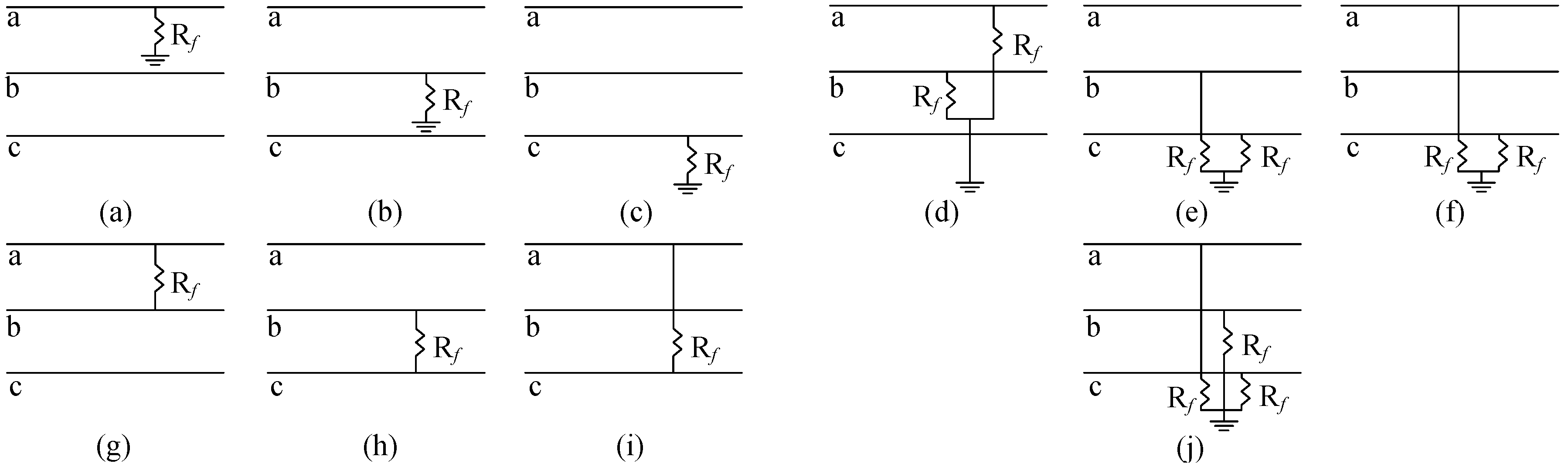
Single LG fault occurs when any phase line of a three phase power line comes in contact with the neutral line or drops to the ground. The fault is also referred to as a short circuit fault caused by heavy wind or the falling of trees on a line. Three types of single line to ground faults are shown in Figure 1a–c, where a, b, and c are three phases of a distribution line.

2.1.2. Two PG Fault

When two lines of a power line fall to the ground, the two PG fault occurs. This fault gives rise to a significant asymmetry and a higher magnitude of fault current compared to the line-to-line fault. If this fault is not cleared in time, it may turn out to be a three line to the ground fault where the severity is much higher than the other types of faults. In Figure 1d–f, the ab-g, bc-g, and ac-g faults are shown where $R_f$ is considered as the fault resistance.

2.1.3. PP Fault

The short circuit between any of the two lines of a three phase system produces this type of fault. One of the important characteristics of this unsymmetrical fault is that the magnitude of the fault impedance varies over a broad range, which makes it difficult to predict its upper and lower limits. Three types of PP faults are presented in Figure 1g–i.

2.1.4. Three PG Fault

3PG fault is a rarely occurring fault, as shown in Figure 1j. This symmetrical fault may be due to the falling of an electric pole or equipment failure. During this fault, the three phase voltage drops to zero, and a large amount of fault current is produced. Though the frequency of occurrence is the lowest, this fault is widely studied in power system protection as the fault produces the maximum amount of short circuit current.

2.2. System Modelling

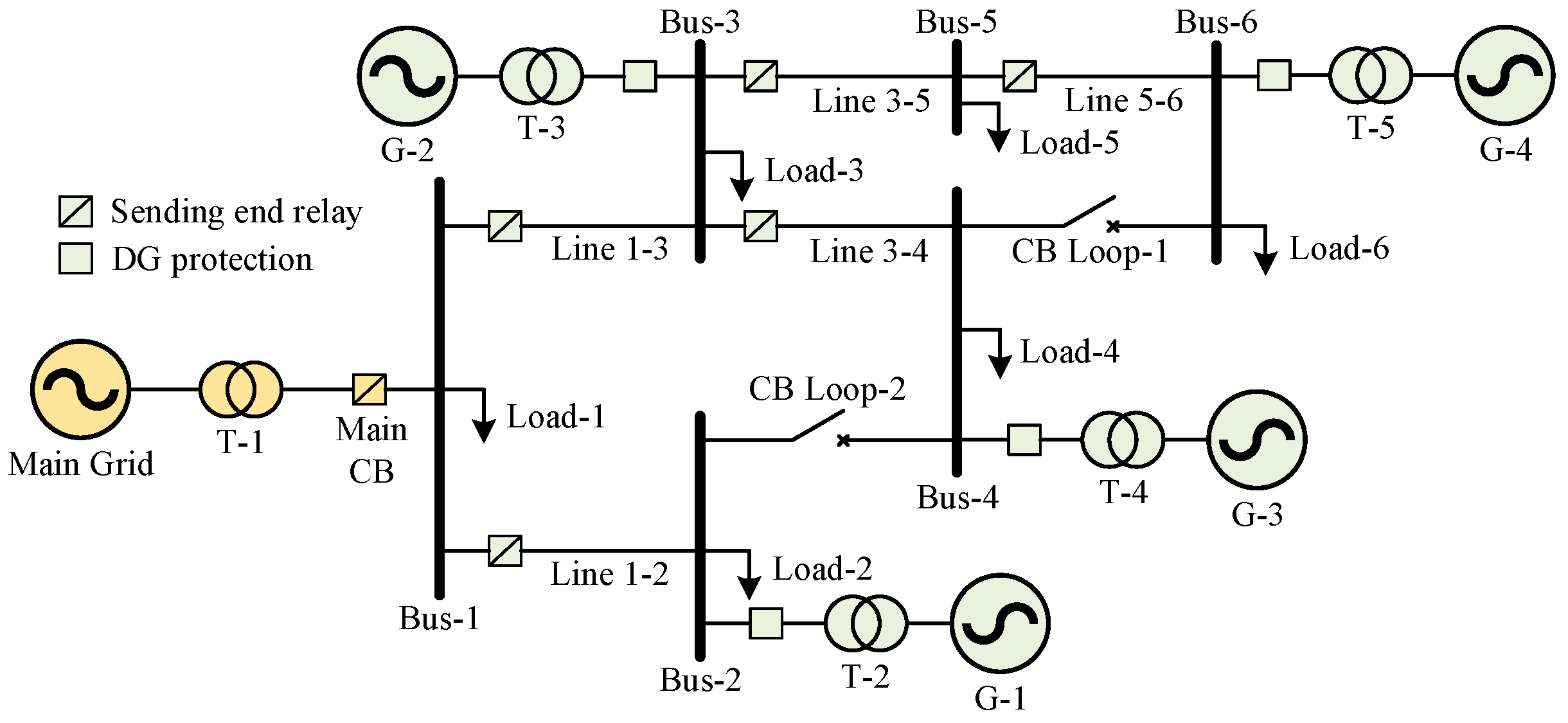
A microgrid system satisfying the International Electrotechnical Commission (IEC) standard [46] was considered in this study to test the classification performance of the proposed network, as illustrated in Figure 2. The studied MG network was modelled in MATLAB/Simulink, which offers extensive facilities to produce the required data. The studied system parameters are reported in

Table 1. Specification of the system parameters.

	System Parameters	Types or Values
Fault	Types of faults	a-g, b-g, c-g, ab-g, bc-g, ac-g, a-b, b-c,
		a-c, abc-g, non-fault
	Fault distance (km)	1 to 19 with an increment of 0.5
	Fault resistance ($\mathsf{\Omega }$)	0.1, 1, 5, 10, 20, 50, 100
Line	Positive and zero sequence resistances ($\mathsf{\Omega }$/km)	0.0135 and 0.0424
	Positive and zero sequence inductances (H/km)	4.9869 × 10−5 and 1.39 × 10−4
	Positive and zero sequence capacitances (F/km)	11.33 × 10−9 and 5.01 × 10−9
	Distance (km): Line 1-3; Line 1-2; Line 3-5; Line 3-4; Line 5-6	20 km each
Transformers (T)	T-1	79/13 kV, 10 MVA, 50 Hz
	T-2 and T-5	0.575/13 kV, 9 MVA, 50 Hz
	T-3 and T-4	0.4/13 kV, 10 MVA, 50 Hz
Generators (G)	Main grid	1000 MVA, 79 kV, 50 Hz
	G-1 (DFIG based wind farm)	Rated MVA: 9 MVA, Rated kV: 575 V
	G-2 (Wind turbine with asynchronous machine)	Rated MVA: 1.5 MVA, Rated kV: 0.4
	G-3 ( Inverter based)	Rated MVA: 10 MVA, Rated kV: 13
	G-4 ( Inverter based)	Rated MVA: 10 MVA, Rated kV: 575 V

. The system carried four DG units of which Generator-1 (G-1) was a DFIG based wind farm, G-2 was a wind turbine with an asynchronous machine, and G-3 and G-4 were inverter based generators. The system frequency was set to 50 Hz, and the base power was considered to be 48 MVA. By having the circuit breaker (CB) at the grid side, the studied system could operate in both modes. Furthermore, changing CB Loop-1 and CB Loop-2 allowed the system to be operated with the looped or radial topology. The distribution lines of the studied system were divided into five sections with a length of 20 km each. Ten types of shunt faults as mentioned in Table 1 were simulated in the distribution lines, and the three phase voltage and currents were sampled from the sending end side of the lines at a sampling rate of 20 kHz. For different network configurations, operating modes, fault distances, fault resistances, and fault inception angles, the signals were sampled for each fault and the non-fault condition to produce the fault data.

2.3. Variation of Signal Energy with Feature Generation

In this paper, a framework of the MG distribution line FDC is proposed based on a probabilistic generative network. For the unhealthy or fault detection plan, the sound or health condition was used to make a type of fault, i.e., including all the short circuit fault conditions and the sound state of phase, presenting a total of 11 fault types. The nature of the classifier was expected to be non-faulty or sound in the healthy condition. An unhealthy or fault event was detected when the classifier output was switched to a distinct fault class. The training of the proposed model demanded digging out the fault features from the raw signals. Every fault signal had a distinct signal energy, which depended on the system parameters, i.e., fault distance and resistance. The variation in raw signals of each phase was separately analysed by applying the DWT. Afterwards, individual signal energy was calculated for preparing the required dataset.

2.3.1. Effect of Fault Distance on Signal Energy

The unhealthy or faulty event may occur at any point of a distribution network. The training approach of the proposed DBN with a variation of the fault distance enabled the network to inspect the signal anywhere in the distribution network. For the sample data generation, the location of the fault event was varied within 1 to 19 km with an increment of 0.5, and the current and voltage waveform were observed. The variation of the raw signal created different lengths of signal energy, which ended up representing various features. For the demonstration, a variation in the signal energy during the a-g fault for different fault locations at Lines 1-3 is presented in Figure 3. From the analysis, the signal energy of the faulted phase current and voltage waveform were observed and varied with the distance. While performing this demonstration, the value of the faulted strength/resistance was fixed to 10 $\mathsf{\Omega }$, while other parameters remained persistent, as mentioned before.

2.3.2. Effect of Fault Resistance on Signal Energy

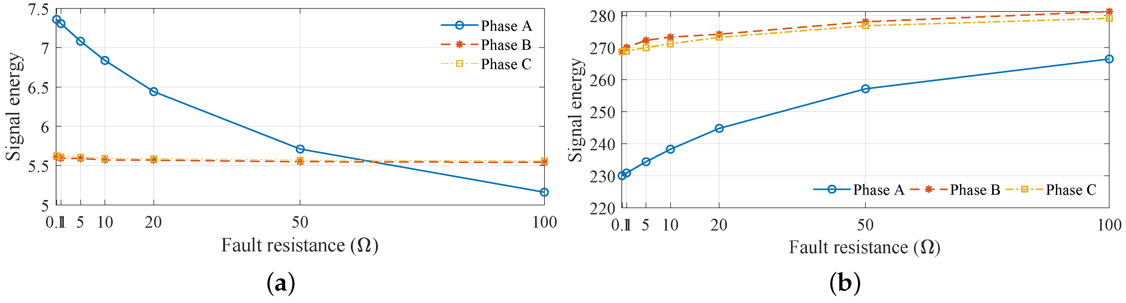
The fault resistance/strength also had a great impact on the raw signals. The short circuit fault event carried with the ground may be responsible for creating inaccurate attribute measurement if the fault strength is not considered. In turn, the proposed FDC system was studied with the difference of the fault strength and training the system for effective FDC. The signal energy from the three phase voltage and current for Lines 1-3 at different fault resistances are shown in Figure 4. From the figure, the energy of the faulty phase was observed, which enabled the system to characterize a fault of different fault resistances. While demonstrating the result of fault resistance/strength on the signal energy, the distance of the fault was set to 10 km from the sampling end, and other parameters remained constant.

2.4. Fault Feature Generation with Wavelet Transform

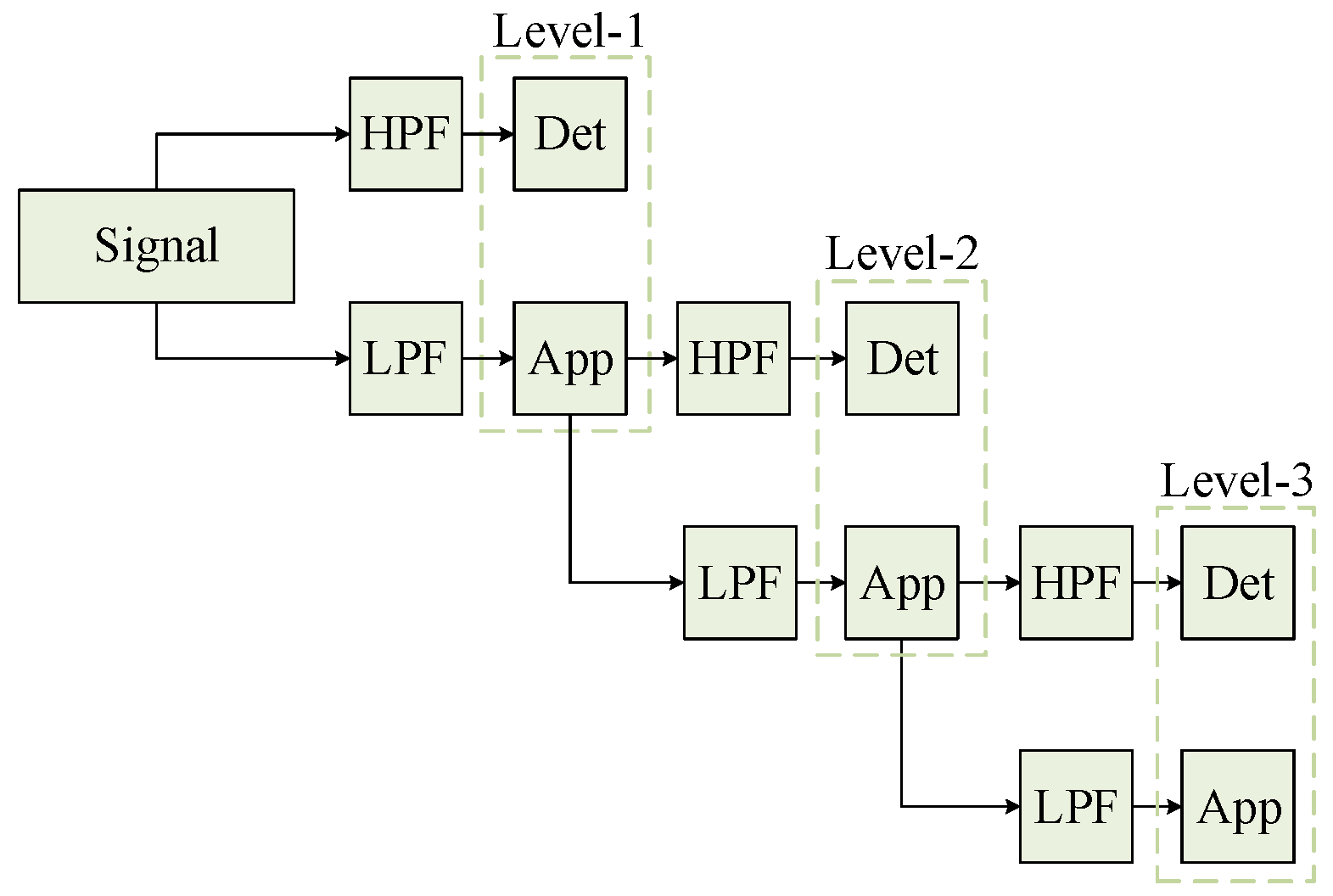
In this study, the DWT was used to explore the features of a distinct portion of a signal when a rapid change in signal occurred. The WT is the decomposition of a signal into a time series of components. The time series faulty components shield a distinct frequency portion, presenting extensive instruction of a time series waveform. In turn, the WT technique is used here to represent the fault attribute of a particular area of the faulty signal during a fault event. In DWT, a signal goes through a series of high-pass filters (HPF) and a low-pass filters (LPF). The LPF analyse the signal at the low-frequency domain, while the HPF analyse the signal high-frequency domain, which as a result disintegrates the signal into detail (Det) and approximation (App) coefficients. The App coefficient depicts the large- and small-scale frequency elements of the fault signal. Accordingly, the Det coefficient represents the small- and large-scale frequency elements of the fault signal. This decomposition process is replicated with the consecutive App so that a fault signal is divided into some smaller resolution sections. This process is referred to as a decomposition tree for DWT, as presented in Figure 5.

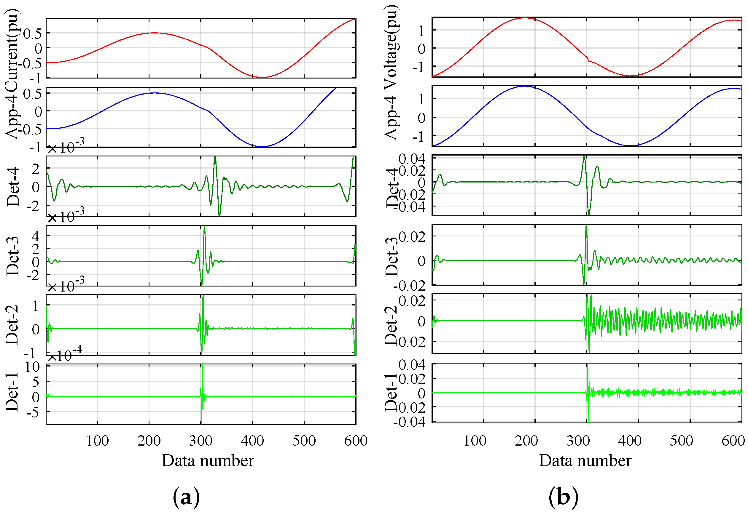
In this research, a $1/2$ cycle post fault current and voltage information were passed through the multi-resolution wavelet block to extract the App and Det level components correlated with the fault current/voltage data. The Daubechies wavelet (DB) was chosen as a mother wavelet as it has been already proven to work effectively [47]. When a short circuit fault occurs in the distribution line, a variation in the wavelet coefficients of the voltage and current waveforms is noted for various system parameters that carry the valuable fault signature information. For illustration, the Line-a current and voltage waveforms in the presence of the a-g fault are analysed with DWT, and the detailed 4-level wavelet coefficients are presented in Figure 6a and Figure 6b, respectively. At the first level, a cutting spike at the fault inception point is noticed, which shows the highest frequency accessible in the faulty voltage and current waveform. These signal spikes are observed every time when a sudden change in the signals occurs. Thus, the identification of these fault signal spikes is not the proper way to identify the faults of the power transmission line. At the fourth level, the Det level coefficient finds that there exists a side-band that carries several smaller spikes. The changing of the system parameters like the fault resistance, fault distance, and fault type is done to observe the high spikes along the obtained side bands. If this process is accomplished beyond these decomposition levels, it is observed to carry higher side-bands, which makes the complex connection among the fault type, inception angle, and fault resistance and location. Therefore, the meaningful attributes are selected from the Det Level-4 coefficient. Using this coefficient, the energy of a signal [48] can be calculated as follows,

$$\begin{array}{c}\hfill E_i=\sum _{j=1}^n{d_{ik}}^2.\end{array}$$

(1)

where $d_{ik}$ is the detail level coefficient of a signal. The term $j=1,2,3,\dots ,n$ stands for the number of points used for each wavelet coefficient, and $i=1,2,3,\dots ,I$ denotes the scale. From [3], it can be concluded that the change in the wavelet coefficient due to the transient events such as faults, in turn, brings a change in the signal energy. The signal energy is calculated for each three phase current and voltage to generate the necessary input features of the proposed FDC model.

$$\begin{array}{cc}\hfill DW{T}_{x,m,n}=& \frac{1}{\sqrt{a_0^m}}\sum _{l}x\left(k\right){\psi }^{\ast }\left(\frac{n-l{a}_0^m{b}_0}{a_0^m}\right),\hfill \end{array}$$

(2)

where l and m present the integer variable and $l{a}_0^m{b}_0$ and $a_0^m$ show the time and scale shift parameter, respectively. The parameters $a_0$ and $b_0$ in (1) were chosen with a value of 2 and 1, respectively.

2.5. Proposed Hierarchical Generative Fault Classification Model

The framework of the deep belief network (DBN) for MG distribution line FDC is introduced in this section. The proposed network consists of a stack of restricted Boltzmann machine (RBM). The use of a stack of RBM turns the network into a deep architecture where the RBM restrains the network to cope with overfitting of the training data.

2.5.1. Restricted Boltzmann Machine

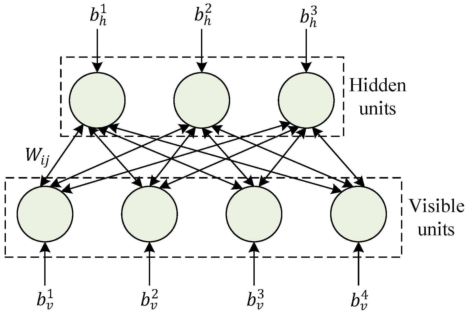
The RBM is a generative probabilistic model with a two layer neural network. The first layer or the data input layer (visible layer) of RBM consists of visible units $u_v$, while the second layer (hidden layer) consists of the hidden units $u_h$. A connection between each visible and hidden unit appears with a weight matrix W that restricts to dealing with any two units of the visible and hidden layer of RBM as shown in Figure 7. The visible and the hidden units have bias vectors $b_v$ and $b_h$, respectively. The energy function for the hidden and visible units is represented as,

$$\begin{array}{cc}\hfill E\left(u_v,u_h\right)=& -\sum _{i=1}^{N_v}\sum _{j=1}^{N_h}{W}_{ij}{u}_v^i{u}_h^j-\sum _{i=1}^{N_v}{b}_v^i{u}_v^i-\sum _{j=1}^{N_h}{b}_h^j{u}_h^j,\hfill \end{array}$$

where $u_v^i\mathrm{and}{u}_h^j$ and $b_v^i\mathrm{and}{b}_h^j$ are the binary states and biases for the $i^{\mathrm{th}}$ visible unit and $j^{\mathrm{th}}$ hidden unit. The number of visible and hidden unit is denoted as $N_v$ and $N_h$. The joint arrangement of the given units can be determined via the energy function as,

$$\begin{array}{cc}\hfill P\left(u_v,u_h\right)=& \frac{1}{Z}{e}^{-E\left(u_v,u_h\right)}.\hfill \end{array}$$

(3)

Here, Z is the partition function that ensures the normalized distribution. The probability of hidden unit $u_h^i$ is activated for the visible vector $U_v$, and the probability of visible unit $u_v^j$ is activated for the hidden vector $U_h$. For the binary state of visible and hidden units, the activation functions are represented as:

$$\begin{array}{cc}\hfill P\left(u_h^j\mid u_v\right)=& \delta \left(b_h^j+\sum _i{W}_{ij}{u}_v^i\right),\hfill \end{array}$$

(4)

$$\begin{array}{cc}\hfill P\left(u_v^i\mid u_h\right)=& \delta \left(b_v^i+\sum _j{W}_{ij}{u}_h^j\right).\hfill \end{array}$$

(5)

Here, $\delta \left(·\right)$ carries the property of the activation function. In (3), the input data from the high-dimensional space are transformed to the low-dimensional space as characteristic vectors (CV). This process is designated as the positive phase learning. The negative phase learning is described in (4) when the input data are reconstructed from the CV. The other parameters W, $b_v$, and $b_h$ are trained concurrently to lessen the reconstruction error. The categorical cross-entropy loss (CL), known as the negative log-likelihood, is a loss function that measures the similarity between the true level and the predicted level as below,

$$\begin{array}{cc}\hfill CL=& -\sum \left(P{D}_{true}\ast log\left(P{D}_{predicted}\right)\right).\hfill \end{array}$$

(6)

The proposed DBN contains the five stacked RBM where the first hidden layer constructs the first RBM. The output of the first RBM is fed to the second RBM combined with the second and third hidden layers. In this way, the data from the input layer flow through the RBM stack and finally reach the final layer. We mention that the first invisible layer of the RBM is the visible layer for the second RBM, and so is the higher layer RBM. A DBN structure with four stacked RBM is displayed in Figure 8.

2.5.2. Unsupervised Learning of the Proposed Network

The training phase of the proposed DBN based fault classifier consisted of pre-training of the layer for the single RBM with an unsupervised approach and tuning of the DBN with the ANN. Initially, each RBM layer was trained by applying the Adam optimization algorithm on the negative log-likelihood probability of the training dataset. The gradient of the negative logarithmic probability for the visible layer in terms of the parameter W is specified as,

$$\begin{array}{cc}\hfill \frac{\delta logP\left(u_v\right)}{\delta W_{ij}}=& {\left(u_v^i{u}_h^j\right)}_{data}-{\left(u_v^i{u}_h^j\right)}_{model},\hfill \end{array}$$

(7)

where ${\left(u_v^i{u}_h^j\right)}_{data}=p$ presents the expectation under the data distribution and ${\left(u_v^i{u}_h^j\right)}_{model}=q$ presents the expectation under the model distribution. The contrastive divergence approximation after the $k^{\mathrm{th}}$ iteration of Gibbs sampling is customarily chosen to train the RBM. If the input $x^r$ is given from a dataset $x^r{\mid }_{r=1}^M$, the Gibbs sampling for one single step is addressed as,

$$\begin{array}{cc}\hfill u_v^{\left(0\right)}\sim & x^r,\hfill \end{array}$$

(8)

$$\begin{array}{cc}\hfill u_h^{\left(0\right)}\sim & P\left(u_h\mid u_v^{\left(0\right)}\right),\hfill \end{array}$$

(9)

$$\begin{array}{cc}\hfill u_v^{\left(1\right)}\sim & P\left(u_v\mid u_h^{\left(0\right)}\right),\hfill \end{array}$$

(10)

$$\begin{array}{cc}\hfill u_h^{\left(1\right)}\sim & P\left(u_h\mid u_v^{\left(1\right)}\right),\hfill \end{array}$$

(11)

and the updated rule for parameter W is given as,

$$\begin{array}{c}\hfill W\leftarrow W+\epsilon \left(\langle u_v^i\left(0\right)u_h^j\left(0\right)\rangle -\langle u_v^i\left(1\right)u_h^j\left(1\right)\rangle \right).\end{array}$$

(12)

2.5.3. Supervised Training of the Proposed Network

The fine-tuning of the model parameters of the DBN structure is performed by utilizing the ANN algorithm to minimize the error between the predicted output and the input samples. Analogous to the unsupervised learning stage, the supervised training is performed by the layer-by-layer training process. Taking weights from the RBM, each neuron in the ANN layer performs the following operation,

$$\begin{array}{cc}\hfill z_k^{\left[j\right]}=& W_k^T·a^{[j-1]}+b_k,\hfill \\ \hfill a_i^{\left[j\right]}=& g\left[j\right]\left(z_k^{\left[j\right]}\right).\hfill \end{array}$$

(13)

where j implies the number of layers in the ANN architecture and i denotes the number of neurons in a single layer. As similar operations have to be performed for each of the ANN layers, the vectorization of the transposed weights $W^T$ is stacked together to form a matrix W. The initialization of these weights is done using “He normal initialization” where the weights are selected randomly, which connect the neurons of the proposed model [49]. After the initialization is done, the model itself updates the weights based on the size of the former layer of the neurons to meet the convergence criteria of the objective function. Similarly, the bias b of each neuron in the ANN layer creates the vertical vector b.

The ReLU function is used to activate all of the process, and the output from (13) is transferred through a non-linear activation function $g_n$ that forms an updated output matrix as,

$$\begin{array}{cc}\hfill {\mathbf{z}}_k^{\left[j\right]}=& {\mathbf{W}}_k^T·{\mathbf{a}}^{[j-1]}+{\mathbf{b}}_k,\hfill \\ \hfill {\mathbf{a}}_i^{\left[j\right]}=& g\left[j\right]\left({\mathbf{z}}_k^{\left[j\right]}\right).\hfill \end{array}$$

(14)

The vectors a and z of each ANN layer create the A, and Z matrices, respectively. From (12), we can write this as:

$$\begin{array}{cc}\hfill {\mathbf{Z}}_k^{\left[j\right]}=& {\mathbf{W}}_k^T·{\mathbf{A}}^{[j-1]}+{\mathbf{b}}_k,\hfill \\ \hfill {\mathbf{A}}_i^{\left[j\right]}=& g\left[j\right]\left({\mathbf{Z}}_k^{\left[j\right]}\right).\hfill \end{array}$$

(15)

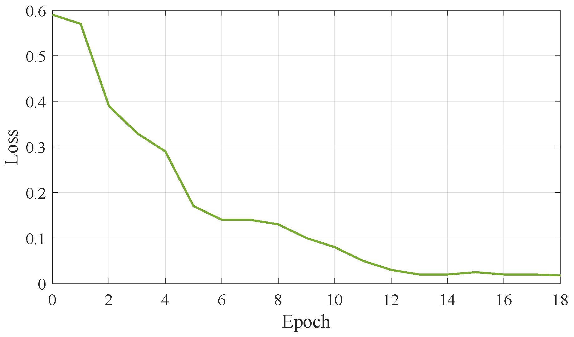
To demonstrate the progress of learning, the model applies the categorical cross-entropy as a loss function, which can be represented in (16). As an example, the loss curve for grid-tied radial mode operation is shown in Figure 9, where the value of the learning coefficient is selected using a trial and error method. The aim of the method is to achieve the maximum training speed by minimizing the loss curve. The losses for all four modes of operation are calculated in a similar manner.

$$\begin{array}{c}\hfill L_i=-\sum _{C=1}^{11}{t}_{i,C}log\left(p_{i,C}\right).\end{array}$$

(16)

Here, $t_{i,C}=1$ if and only if i belongs to class C, and $p_{i,c}$ is the output probability of i belonging to class c. To go from correct class y where the arbitrary values $y\in {\mathbb{R}}_C$ to normalized probability estimates $p\in {\mathbb{R}}_C$ for a single instance, we can write,

$$\begin{array}{c}\hfill p_i=\frac{exp{y}_i}{{\sum }_{C=1}^{C}exp{y}_C},\end{array}$$

(17)

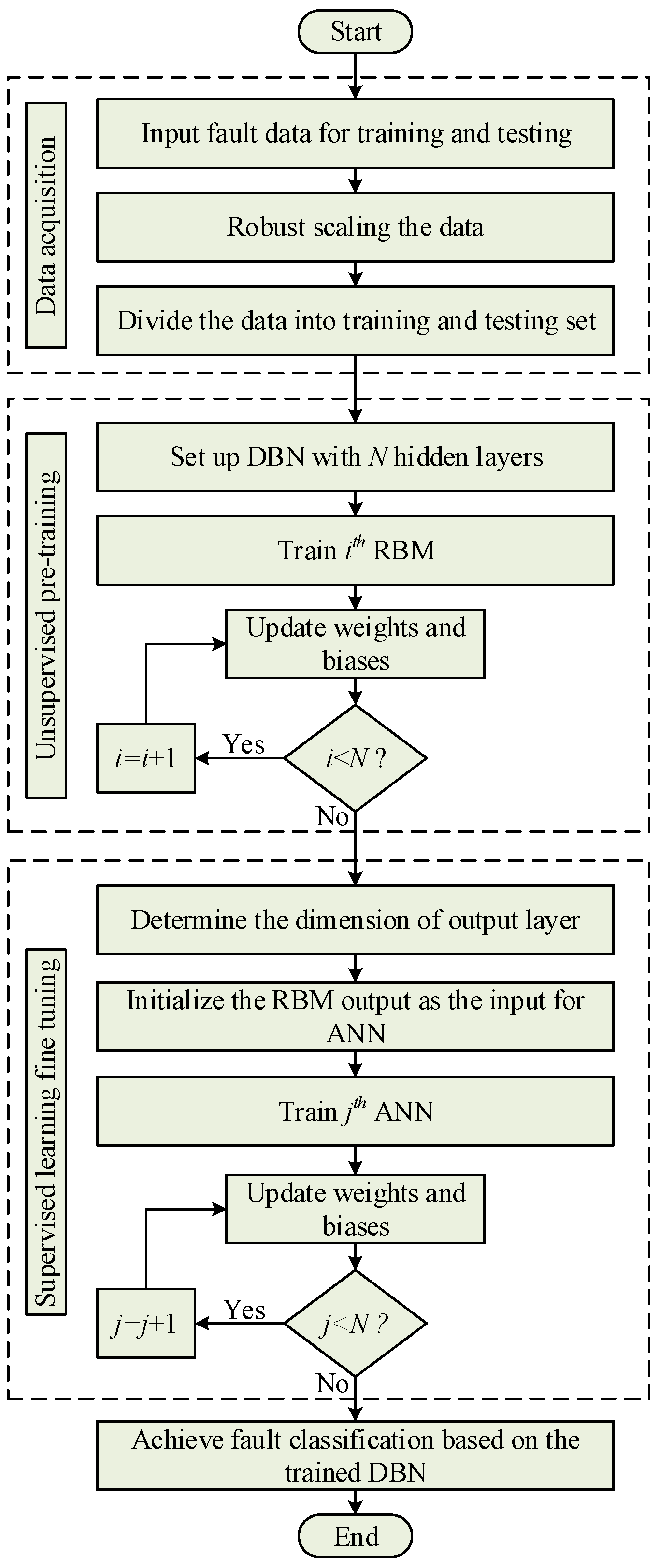
where i and $C\in \{1,\dots ,C\}$ show the class range and $p_i,y_1$ and $y_C$ refer to the class probabilities and values for a single instance. A program flowchart of the DBN based fault detection and classification scheme showing the entire process is given in Figure 10.

3. Results and Discussion

This section illustrates the performance of the proposed fault detection and classification technique with different parameter variations. The fault current and voltage signals exposed dissimilar magnitudes in islanded mode and grid-connected mode. Thus, it was difficult to design a unified fault classification scheme. Therefore, the performance of the proposed model was individually analysed for different system topologies (radial or loop) and operating modes (grid-connected or islanded). The accuracy was evaluated by three aspects: (i) type of input signal, i.e., how the system performed with only the current or voltage waveform and with the voltage and current waveforms combined; (ii) sampling resolution, i.e., system accuracy evaluation with a variety of data acquirement rates; (iii) fault signal with noise present in it, i.e., the system performance with the noise present in the sampled signal. Additionally, a comparative analysis in terms of the accuracy of the existing and proposed FDC techniques was also carried out to show the superior short circuit fault classification performance of the proposed classifier.

3.1. Performance Assessment of the DBN Based FDC Scheme

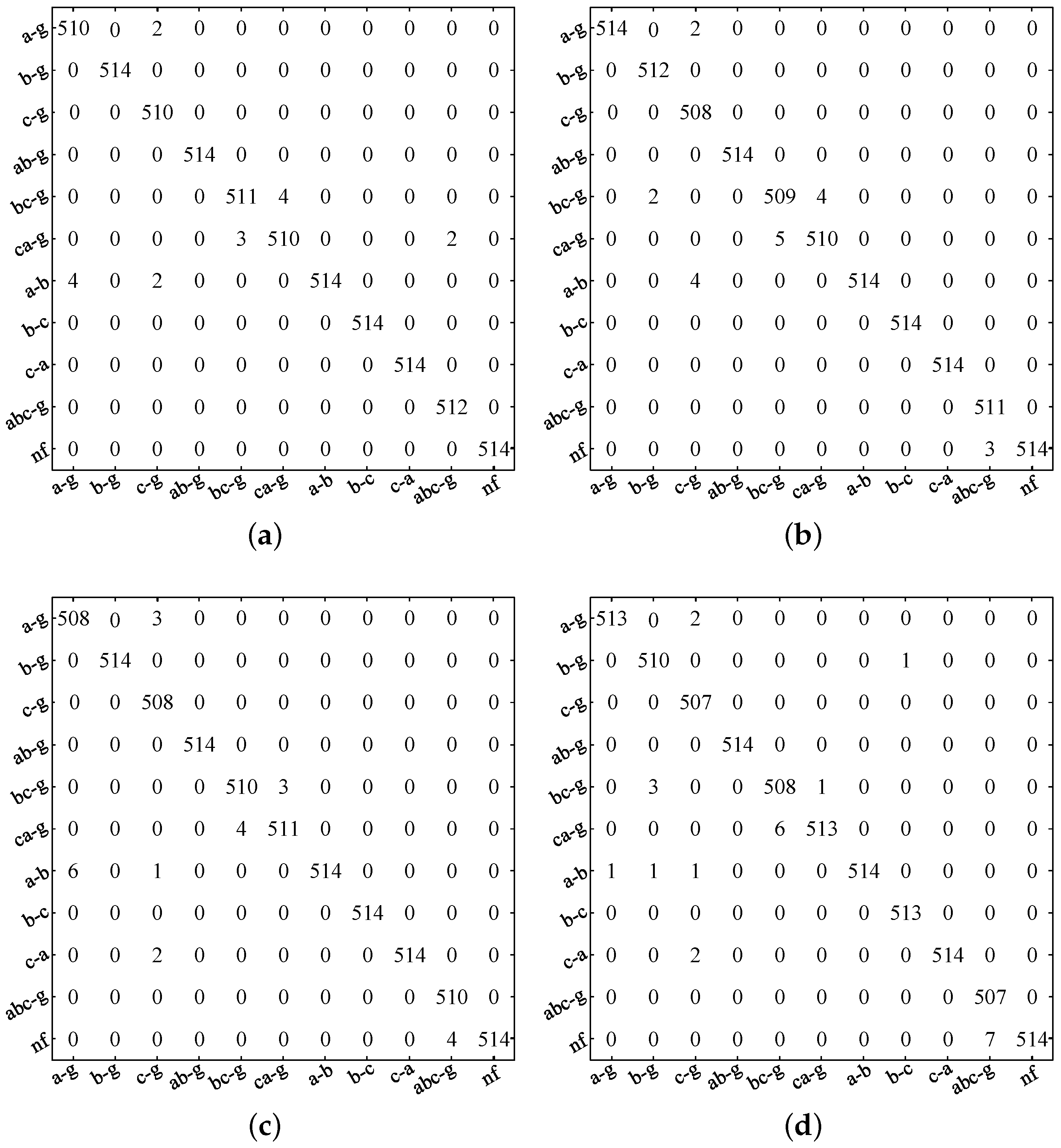
In machine learning, to measure the validity of a learning model, a list of the data sample to test the model performance is used, which should be different from the training data [50]. As a total of 1716 samples was made from the current and voltage waveforms for the individual datasets, it was first mixed and shuffled, and then, 30% of the data was randomly selected to test the effectiveness of the proposed model. The performance of the proposed DBN for Lines 1-3 was simulated with different system configurations and operating modes of MG and illustrated in Figure 11 with the confusion matrix (CM) where the 11 different fault classer were inserted into the x- and y-axis in the form of an $11\times 11$ matrix. The horizontal levels represent the actual class, whereas the vertical levels represent the predicted fault class. The confusion matrix also reports the count of true positives (TP), true negative (TN), false positives (FP), and false negatives (FN), which are defined as:

• TP: A label is correctly predicted by the classifier, and it belongs to the original class.
• TN: A label is correctly predicted by the classifier, and it does not belong to the original class.
• FP: A label is predicted as positive by the classifier. but it does not belong to the original class.
• FN: A label is predicted as negative by the classifier, but it belongs to the original class.

Primarily, from the CM, it was seen that most of the fault classes for all system configuration were classified correctly. The first accuracy measurement criterion from the confusion matrix was the average classification accuracy (AA) [51] as stated in (18).

$$\begin{array}{c}\hfill AA=\frac{TN+TP}{TN+TP+FN+FP}=\frac{N_{TD}}{N_{CC}}.\end{array}$$

(18)

Here, $N_{TD}$ presents the total number of input data for the developed model, and $N_{CC}$ implies the number of correctly classified data. The proposed network could also show a similar performance for the rest of the distribution line. The average accuracy calculated for all of the distribution line is depicted in

Table 2. Average accuracy for different system configurations.

System Configuration	Average Accuracy(%)
	Line 1-3	Line 1-2	Line 3-4	Line 3-5	Line 5-6
Grid-connected radial mode	99.70	99.71	99.36	99.68	99.21
Grid-connected loop mode	99.65	99.69	99.35	99.62	99.07
Islanded radial mode	99.59	99.48	99.13	99.42	98.80
Islanded loop mode	99.56	99.51	98.97	99.39	98.82

. From the result, the highest accuracy of the proposed classifier was recorded as 99.70% for the grid-connected radial mode operation. For the other system configurations, the classifier performed better than 99.5%, which was in line with the expectation.

However, the average accuracy could not present the detailed result about the model performance. Thus, to investigate how the classifier behaved for individual fault classes, the classification performance was further assessed with the F1-score. The F1-score is a function of precision and recall/sensitivity, which is considered as perfect when its value is one and the worst if it is zero. The precision, which is known as the positive predictive value, can be defined as,

$$\begin{array}{c}\hfill Precision=\frac{TP}{TP+FP}.\end{array}$$

(19)

For a good classifier, the precision value should be one. From (19), if the FP increases, the precision value decreases, which is not expected for a good classifier. Another metric, recall, which is known as the true positive rate or the sensitivity of the classifier, can be defined as,

$$\begin{array}{c}\hfill Recall=sensitivity=\frac{TP}{TP+FN}.\end{array}$$

(20)

Like the precision, the recall value should be one for a good classifier. For this metric, if the FN increased, the recall value decreased, which was also not in line with the expectation. Therefore, another performance evaluation metric known as the F1-score was adopted, which takes both precision and recall into account. The higher F1 score of the proposed classifier for both voltage and current signals depicted in

Table 3. Precision, recall, F1-score, and individual class accuracy of the proposed classifier for grid-connected radial mode and grid-connected loop mode operation.

Fault Class	Radial Mode				Loop Mode
	Accuracy (%)	Precision	Recall	F1-Score	Accuracy (%)	Precision	Recall	F1-Score
a-g	99.89	1.0	0.99	0.99	99.96	1.0	1.0	1.0
b-g	100	1.0	1.0	1.0	99.96	1.0	1.0	1.0
c-g	99.93	1.0	0.99	1.0	99.89	1.0	0.99	0.99
ab-g	100	1.0	1.0	1.0	100	1.0	1.0	1.0
bc-g	99.88	0.99	0.99	0.99	99.81	0.99	0.99	0.99
ac-g	99.84	0.99	0.99	0.99	99.84	0.99	0.99	0.99
a-b	99.89	0.99	1.0	0.99	99.93	0.99	1.0	1.0
b-c	100	1.0	1.0	1.0	100	1.0	1.0	1.0
a-c	100	1.0	1.0	1.0	100	1.0	1.0	1.0
abc-g	99.96	1.0	1.0	1.0	99.95	1.0	0.99	1.0
nf	100	0.99	1.0	1.0	99.95	0.99	1.0	1.0

and

Table 4. Precision, recall, F1-score, and individual class accuracy of the proposed classifier for islanded radial mode and islanded loop mode operation.

Fault Class	Radial Mode				Loop Mode
	Accuracy (%)	Precision	Recall	F1-Score	Accuracy (%)	Precision	Recall	F1-Score
a-g	99.84	0.99	0.99	0.99	99.95	1.0	1.0	1.0
b-g	100	1.0	1.0	1.0	99.91	1.0	0.99	1.0
c-g	99.89	1.0	0.99	0.99	99.91	1.0	0.99	1.0
ab-g	100	1.0	1.0	1.0	100	1.0	1.0	1.0
bc-g	99.88	0.99	0.99	0.99	99.82	0.99	0.99	0.99
ac-g	99.88	0.99	0.99	0.99	99.88	0.99	1.0	0.99
a-b	99.98	0.99	1.0	0.99	99.95	0.99	1.0	1.0
b-c	100	1.0	1.0	1.0	99.95	1.0	1.0	1.0
a-c	99.96	1.0	1.0	1.0	100	1.0	1.0	1.0
abc-g	99.93	1.0	0.99	1.0	99.88	1.0	0.99	0.99
nf	99.93	0.99	1.0	1.0	99.88	0.99	1.0	0.99

showed that the classifier had less problems with the false positives and false negatives. Furthermore, from the classification accuracy (user accuracy) for each fault class, it could be concluded that the classifier had the ability to classify the faults with high accuracy.

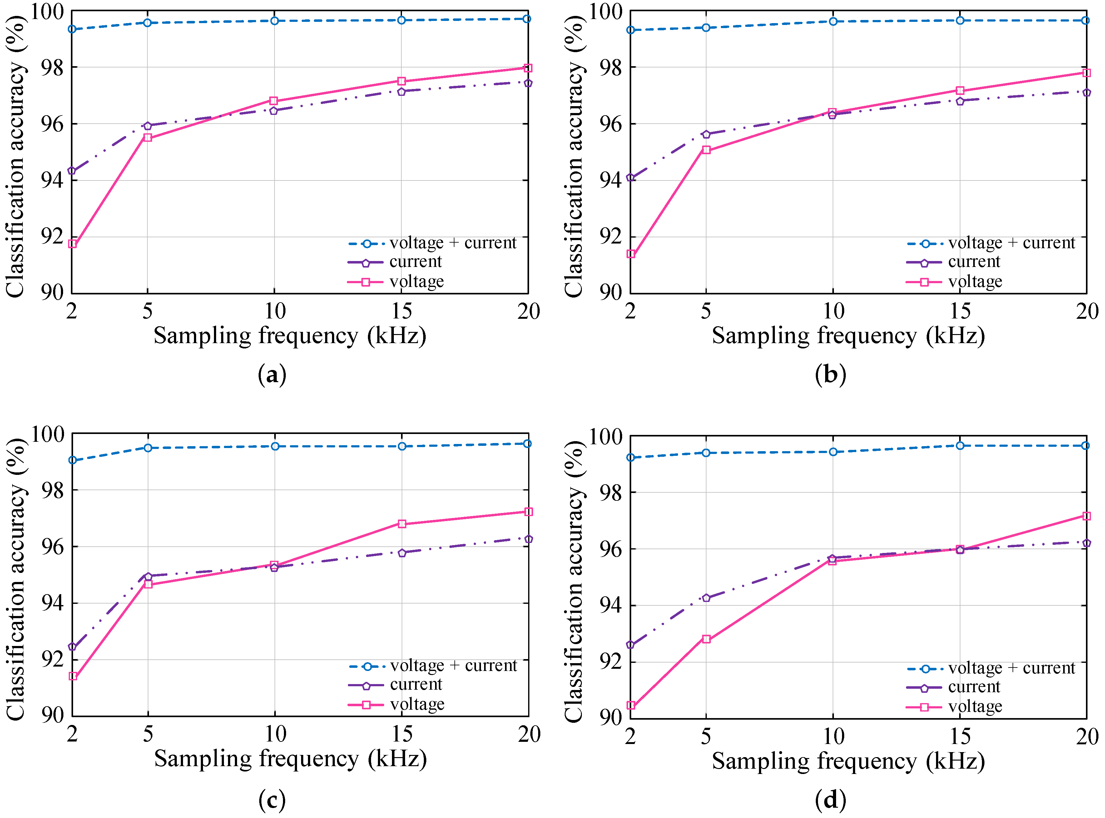
3.2. Effect of Sampling Resolution and Signal Type

In the proposed FDC method, the three phase current and voltage waveforms were collected with a 20 kHz sampling resolution. In reality, the sampling frequency (SF) can be much less than 20 kHz because of the restrictions of the data collection apparatus. In some practical field scenarios, the FDC system needs to utilize current or voltage waveforms to perform the classification tasks due to the unavailability of both signals at the same time instance. Thus, the fault classification performance of the proposed classifier was examined with the variation of input signal type, as well as sampling rate. The SF utilized in this research were 2, 5, 10, 15, and 20 kHz, and the input signal types were the voltage waveform (Scheme-1) or current waveform (Scheme-2) and combined current and voltage waveform (Scheme-3). The classification results for an SF and a particular type of signal was done by performing the classification process five times. Thereafter, the mean value of the accuracies was determined to achieve the final results as shown in Figure 12.

The increase in classification accuracy was expected as a higher SF carried more detailed fault information for a distinct short circuit fault class. Moreover, Scheme-3 offered the highest classification performance for all considered SF. At a smaller sampling rate, better classification performance was observed with the three phase current waveform than with the three phase voltage waveform. Furthermore, the FDC system performed better with the voltage signal information at a higher SF. At an SF range between 5 kHz and 10 kHz, Scheme-2 and Scheme-3 showed almost the same classification accuracy. This scenario was also expected, as the voltage waveform carried less low-frequency fault information than the current waveform for a distinct fault class. On the other side, the voltage waveform contained spare faulted transients, which were suitable to investigate the type of short circuit fault at the higher sampling rate. The above analysis explicated that the expected accuracy could not be accomplished with only the current or voltage waveform. If both waveforms were considered at a time, a higher fault classification performance could be accomplished within the considered frequency level as particular short circuit fault information for both the three phase current and voltage intents was used. From the aforementioned study, it was observed that the classification accuracy using only the current or voltage waveform was not satisfying; rather, their fusion offered more than a 99% classification accuracy at the large level of the considered frequency range, which validated the effectiveness of the proposed FDC model. The similar classification results could also be observed for the rest of the distribution line of the studied MG system.

3.3. Effect of Noise Present in the Measured Signal Data on the Classification Accuracy

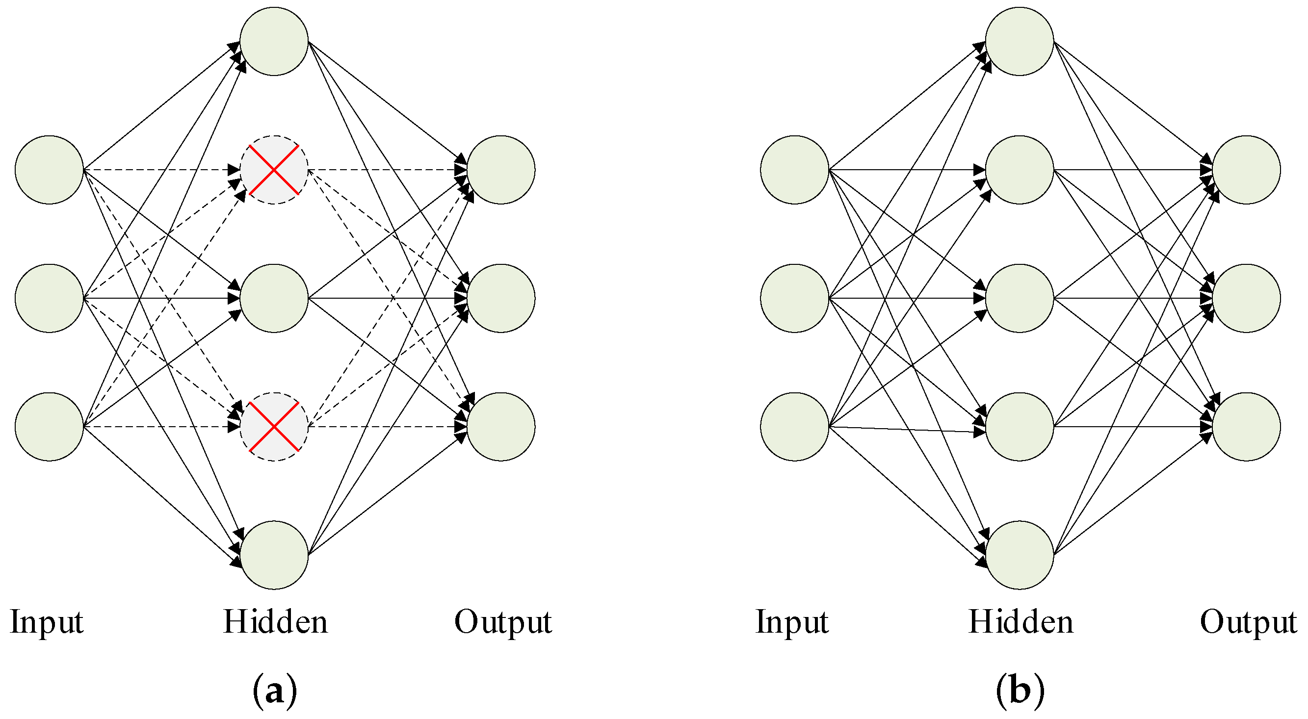
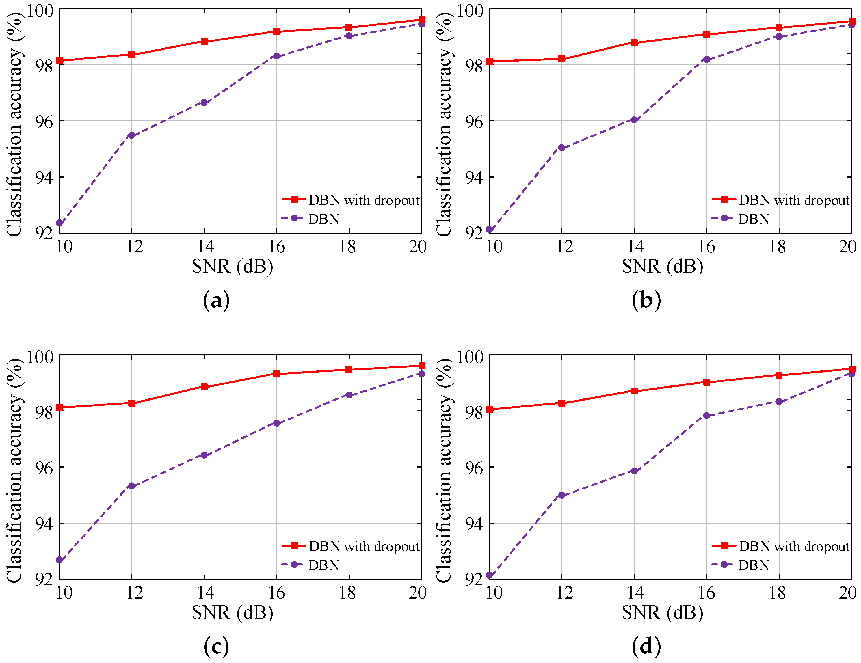
In practice, the current or voltage waveforms are continuously subjected to statistical noises or uncertainties, which play an important role in degrading the overall performance of the MG fault diagnosis. Thus, the dropout strategy was added to the hidden layer of the RBM to confirm the performance [52]. The fundamental idea of dropout is that it randomly sets the hidden nodes to zero at a certain probability to prevent overfitting of the model. That means some nodes present in the hidden layer do not engage in the training phase, and the weights will be reserved. The ignored nodes will be involved again in the next iteration. Thus, for each iteration process, the dropout strategy removes some random nodes of the hidden layer from the network. This process can effectively restrain the interdependence among the features and enhances the noise-immune classification performance. A comparison of the network structure with and without the dropout strategy is shown in Figure 13.

To examine how the proposed model could show the result with noisy data, the system was run with a new sample dataset, which contained both signals (current and voltage). To validate the model performance with the noisy data, the white Gaussian noise of different signal-to-noise ratios (SNR) as per [53] was added with 30% of the test data from the main dataset. Now, the proposed classifier was trained with the original data and tested with the contaminated data. The performance of the proposed classifier with the contaminated data is shown in Figure 14. From the result, it was observed that the fault classification performance of the proposed FDC model with the dropout strategy was higher than the model without dropout. The classification performance without the dropout strategy was observed to decrease faster with the decrement of the SNR value for each mode of MG operation, as shown in Figure 14. Finally, it was concluded that the classification accuracy against the noise guaranteed the robust performance of the proposed classifier.

3.4. Comparative Study

A comparison among the proposed model and several existing alternative fault diagnosis models is discussed in this section. In [30], a discrete orthonormal S-transform based multi-kernel extreme learning machine (MKELM) was proposed and compared with KELM and SVM. The mentioned approaches use only the one cycle post fault current signal to declare a fault type that cannot confirm the accurate results at a lower SF, as discussed in Section 3.2. However, comparing the proposed approach with the existing approaches is not fully consistent because of the following aspects. This research analysed the faults occurring in the considered MG for different topologies, i.e., looped or radial, operating modes, i.e., islanded or grid-tied, and for different distribution lines, separately. Therefore, the result analysis carried out in this study was much more challenging due to the diversity of the system parameters. Even though the results were not directly comparable, a comparison of the classification performance with the methods mentioned in [30] is depicted in

Table 5. Comparison of the classification performance between the proposed and existing fault detection and classification (FDC) methods.

SNR	Classification Accuracy (%)
	MKELM	KELM	SVM	DBN with Dropout
30 dB	98.29	98.15	98.24	99.38

. It was observed that the accuracy of the proposed approach was better than the other approaches. Again, the classification accuracy discussed in Section 3.3 for the lower value of SNR proved the noise-immune performance of the proposed method. Additionally, the DBN based FDC scheme had a superior feature over the conventional and modern FDC techniques, as illustrated in

Table 6. Comparison of the advantages between the existing and the proposed FDC methods.

Techniques	Methods	Advantages	Disadvantages
Classical strategies	Circuit theory,	1. Simplicity	1. Inaccurate
	Traveling waves,	2. Easy implementation	2. Limited fault type
	Symmetrical		classification
	component		3. Slow
Signal processing	FFT,	1. Direct fault analysis	1. Decision threshold are
	WT	2. Used for feature extraction	defined arbitrarily
		and information compression
Statistical	Traditional statistical	1. High generalizability	1. Take longer time to
	concepts	2. Individual data patterns	make a decision
		are clear and visible	2. Validation of data
			is not guaranteed
Knowledge based		1. High precision	1. The accuracy can not be
	Fuzzy logic	2. Rapid operation	guaranteed as the system is
		3. Can handle uncertainty	based on the experts’
			experience
Artificial intelligence		1. Detects the non-linear	1. Slow convergence of
		relationship between	training process
	ANN	independent and dependent	2. Shallow architecture limit the
		variables	capacity to learn the complex
			non-linear relationships
		1. Faster, even if the problem	1. Choosing kernel function and
	SVM	is large-size	hyper parameters are difficult
		2. Requires less heuristics
		1. Good at noisy environment	1. Processes are random
		2. The simulation speed can	2. Outputs are not consistent
	GANN	be improved
		3. Dimension of solution can
		be reduced
Proposed method		1. Robust hierarchical generative
		model
	DBN	2. Restrain overfitting of the
		training data
		3. Discover the fundamental
		regularity of versatile features
		4. Powerful generalization
		capability

.

4. Conclusions

This paper proposed the design of a novel machine learning model that combined the RBM and ANN techniques to detect and classify the faults for both grid-tied and islanded modes of operation of the MG robustly. The novel design of the proposed model combining the RBM and ANN methods guaranteed the model inherently learned and analysed unnatural signals corresponding to different faults that occurred in the MG. This was done by the unique measurement of both the current and voltage waveforms using a DWT against the variation of the line parameters. The use of both the current and voltage elements for FDC attested to the proposed model as a generalized model that worked in various sampling frequencies. The proposed model was tested for measuring the effectiveness by conducting a number of studies like the effect of the signal type, the effect of noise, and the effect of the sampling rates. The results indicated that the proposed FDC model detected and classified the short circuit faults with an accuracy close to 100% for all fault types. This signified the impressive performance of the model designed by employing both the current and voltage waveforms within the studied frequency band. The classification performance of the proposed model was further examined to ensure the robustness against the unwanted noise, and it was shown that the proposed model continued detecting faults against such incorporation of the noise. A comparative analysis between some of the existing models available in the literature and the proposed model was conducted considering a number of instances such as the types of input signals utilized and the level of the signal-to-noise ratio. The comparative analysis showed that the proposed model provided a more stable and trustworthy classification performance as compared to the state-of-the-art. The future implementation of this research may reflect the real-time system data collected by the measuring apparatus and deployed in a real-world power grid.

References

- Mishra, M.; Sahani, M.; Rout, P. An islanding detection algorithm for distributed generation based on Hilbert–Huang transform and extreme learning machine. Sustain. Energy Grids Netw. 2017, 9, 13–26. [Google Scholar] [CrossRef]
- Shuai, Z.; Sun, Y.; Shen, Z.J.; Tian, W.; Tu, C.; Li, Y.; Yin, X. Microgrid stability: Classification and a review. Renew. Sustain. Energy Rev. 2016, 58, 167–179. [Google Scholar] [CrossRef]
- Mishra, D.P.; Samantaray, S.R.; Joos, G. A combined wavelet and data-mining based intelligent protection scheme for microgrid. IEEE Trans. Smart Grid 2015, 7, 2295–2304. [Google Scholar] [CrossRef]
- Parhizi, S.; Lotfi, H.; Khodaei, A.; Bahramirad, S. State of the art in research on microgrids: A review. IEEE Access 2015, 3, 890–925. [Google Scholar] [CrossRef]
- El-Zonkoly, A.M. Fault diagnosis in distribution networks with distributed generation. Electr. Power Syst. Res. 2011, 81, 1482–1490. [Google Scholar] [CrossRef]
- Mishra, M.; Rout, P.K. Detection and classification of micro-grid faults based on HHT and machine learning techniques. IET Gener. Transm. Distrib. 2017, 12, 388–397. [Google Scholar] [CrossRef]
- Memon, A.A.; Kauhaniemi, K. A critical review of AC Microgrid protection issues and available solutions. Electr. Power Syst. Res. 2015, 129, 23–31. [Google Scholar] [CrossRef]
- Ray, P.K.; Panigrahi, B.K.; Rout, P.K.; Mohanty, A.; Eddy, F.Y.; Gooi, H.B. Detection of islanding and fault disturbances in microgrid using wavelet packet transform. IETE J. Res. 2019, 65, 796–809. [Google Scholar] [CrossRef]
- Dey, A.N.; Panigrahi, B.K.; Kar, S.K. Smartgrids/Microgrids in India: A Review on Relevance, Initiatives, Policies, Projects and Challenges. In Innovation in Electrical Power Engineering, Communication, and Computing Technology; Springer: Singapore, 2020; pp. 465–474. [Google Scholar]
- Shi, S.; Jiang, B.; Dong, X.; Bo, Z. Protection of microgrid. In Proceedings of the 10th IET International Conference on Developments in Power System Protection (DPSP 2010), Manchester, UK, 29 March–1 April 2010; pp. 1–4. [Google Scholar]
- Laaksonen, H.J. Protection principles for future microgrids. IEEE Trans. Power Electron. 2010, 25, 2910–2918. [Google Scholar] [CrossRef]
- Agüero, J.R.; Wang, J.; Burke, J.J. Improving the reliability of power distribution systems through single-phase tripping. In Proceedings of the IEEE PES T&D 2010, New Orleans, LA, USA, 19–22 April 2010; pp. 1–7. [Google Scholar]
- Eslami, R.; Sadeghi, S.H.H.; Askarian-Abyaneh, H.; Nasiri, A. A novel method for fault detection in future renewable electric energy delivery and management microgrids, considering uncertainties in network topology. Electr. Power Compon. Syst. 2017, 45, 1118–1129. [Google Scholar] [CrossRef]
- James, J.; Hou, Y.; Lam, A.Y.; Li, V.O. Intelligent fault detection scheme for microgrids with wavelet based deep neural networks. IEEE Trans. Smart Grid 2017, 10, 1694–1703. [Google Scholar]
- Prasad, A.; Edward, J.B.; Ravi, K. A review on fault classification methodologies in power transmission systems: Part—I. J. Electr. Syst. Inf. Technol. 2018, 5, 48–60. [Google Scholar] [CrossRef]
- Magdy, G.; Shabib, G.; Elbaset, A.A.; Mitani, Y. A novel coordination scheme of virtual inertia control and digital protection for microgrid dynamic security considering high renewable energy penetration. IET Renew. Power Gener. 2018, 13, 462–474. [Google Scholar] [CrossRef]
- Zhang, Y.; Wei, W. Decentralised coordination control strategy of the PV generator, storage battery and hydrogen production unit in islanded AC microgrid. IET Renew. Power Gener. 2020, 14, 1053–1062. [Google Scholar] [CrossRef]
- Al Hassan, H.A.; Reiman, A.; Reed, G.F.; Mao, Z.H.; Grainger, B.M. Model based fault detection of inverter based microgrids and a mathematical framework to analyse and avoid nuisance tripping and blinding scenarios. Energies 2018, 11, 2152. [Google Scholar] [CrossRef] [Green Version]
- Hare, J.; Shi, X.; Gupta, S.; Bazzi, A. Fault diagnostics in smart micro-grids: A survey. Renew. Sustain. Energy Rev. 2016, 60, 1114–1124. [Google Scholar] [CrossRef]
- Fahim, S.R.; Sarker, Y.; Islam, O.K.; Sarker, S.K.; Ishraque, M.F.; Das, S.K. An Intelligent Approach of Fault Classification and Localization of a Power Transmission Line. In Proceedings of the 2019 IEEE International Conference on Power, Electrical, and Electronics and Industrial Applications (PEEIACON), Dhaka, Bangladesh, 29 November–1 December 2019; pp. 53–56. [Google Scholar]
- Fahim, S.R.; Sarker, Y.; Sarker, S.K.; Sheikh, M.R.I.; Das, S.K. Self attention convolutional neural network with time series imaging based feature extraction for transmission line fault detection and classification. Electr. Power Syst. Res. 2020, 187, 106437. [Google Scholar] [CrossRef]
- Wan, H.; Li, K.; Wong, K. An multi-agent approach to protection relay coordination with distributed generators in industrial power distribution system. In Proceedings of the Fourtieth IAS Annual Meeting, Conference Record of the 2005 Industry Applications Conference, Kowloon, Hong Kong, China, 2–6 October 2005; Volumbe 2, pp. 830–836. [Google Scholar]
- Sortomme, E.; Venkata, S.; Mitra, J. Microgrid protection using communication-assisted digital relays. IEEE Trans. Power Deliv. 2009, 25, 2789–2796. [Google Scholar] [CrossRef]
- Oh, Y.S.; Kim, C.H.; Gwon, G.H.; Noh, C.H.; Bukhari, S.B.A.; Haider, R.; Gush, T. Fault detection scheme based on mathematical morphology in last mile radial low voltage DC distribution networks. Int. J. Electr. Power Energy Syst. 2019, 106, 520–527. [Google Scholar] [CrossRef]
- Al-Nasseri, H.; Redfern, M.; Li, F. A voltage based protection for micro-grids containing power electronic converters. In Proceedings of the 2006 IEEE Power Engineering Society General Meeting, Montreal, QC, Canada, 18–22 June 2006; p. 7. [Google Scholar]
- Hooshyar, A.; El-Saadany, E.F.; Sanaye-Pasand, M. Fault type classification in microgrids including photovoltaic DGs. IEEE Trans. Smart Grid 2015, 7, 2218–2229. [Google Scholar] [CrossRef]
- Al-Nasseri, H.; Redfern, M. Harmonics content based protection scheme for micro-grids dominated by solid state converters. In Proceedings of the 2008 12th International Middle-East Power System Conference, Aswan, Egypt, 12–15 March 2008; pp. 50–56. [Google Scholar]
- Yadav, A.; Dash, Y. An overview of transmission line protection by artificial neural network: Fault detection, fault classification, fault location, and fault direction discrimination. Adv. Artif. Neural Syst. 2014, 2014, 230382. [Google Scholar] [CrossRef] [Green Version]
- Hong, Y.Y.; Wei, Y.H.; Chang, Y.R.; Lee, Y.D.; Liu, P.W. Fault detection and location by static switches in microgrids using wavelet transform and adaptive network based fuzzy inference system. Energies 2014, 7, 2658–2675. [Google Scholar] [CrossRef] [Green Version]
- Gush, T.; Bukhari, S.B.A.; Mehmood, K.K.; Admasie, S.; Kim, J.S.; Kim, C.H. Intelligent Fault Classification and Location Identification Method for Microgrids Using Discrete Orthonormal Stockwell Transform-Based Optimized Multi-Kernel Extreme Learning Machine. Energies 2019, 12, 4504. [Google Scholar] [CrossRef] [Green Version]
- Gururani, A.; Mohanty, S.R.; Mohanta, J.C. Microgrid protection using Hilbert–Huang transform based-differential scheme. IET Gener. Transm. Distrib. 2016, 10, 3707–3716. [Google Scholar] [CrossRef]
- Kar, S.; Samantaray, S.; Zadeh, M.D. Data-mining model based intelligent differential microgrid protection scheme. IEEE Syst. J. 2015, 11, 1161–1169. [Google Scholar] [CrossRef]
- Ray, P.K.; Mohanty, S.R.; Kishor, N. Disturbance detection in grid-connected distributed generation system using wavelet and S-transform. Electr. Power Syst. Res. 2011, 81, 805–819. [Google Scholar] [CrossRef]
- Manohar, M.; Koley, E.; Ghosh, S. Microgrid protection under wind speed intermittency using extreme learning machine. Comput. Electr. Eng. 2018, 72, 369–382. [Google Scholar] [CrossRef]
- Abdelgayed, T.S.; Morsi, W.G.; Sidhu, T.S. Fault detection and classification based on co-training of semisupervised machine learning. IEEE Trans. Ind. Electron. 2017, 65, 1595–1605. [Google Scholar] [CrossRef]
- Hong, Y.Y.; Cabatac, M.T.A.M. Fault Detection, Classification, and Location by Static Switch in Microgrids Using Wavelet Transform and Taguchi-Based Artificial Neural Network. IEEE Syst. J. 2019, 14, 2725–2735. [Google Scholar] [CrossRef]
- Fahim, S.R.; Datta, D.; Sheikh, M.R.I.; Dey, S.; Sarker, Y.; Sarker, S.K.; Badal, F.R.; Das, S.K. A Visual Analytic in Deep Learning Approach to Eye Movement for Human-Machine Interaction Based on Inertia Measurement. IEEE Access 2020, 8, 45924–45937. [Google Scholar] [CrossRef]
- Sarker, Y.; Fahim, S.R.; Sarker, S.K.; Badal, F.R.; Das, S.K.; Mondal, M.N.I. A Multidimensional Pixel-wise Convolutional Neural Network for Hyperspectral Image Classification. In Proceedings of the 2019 IEEE International Conference on Robotics, Automation, Artificial-Intelligence and Internet-of-Things (RAAICON), Dhaka, Bangladesh, 29 November–1 December 2019; pp. 104–107. [Google Scholar]
- Fahim, S.R.; Sarker, Y.; Rashiduzzaman, M.; Islam, O.K.; Sarker, S.K.; Das, S.K. A Human-Computer Interaction System Utilizing Inertial Measurement Unit and Convolutional Neural Network. In Proceedings of the 2019 5th International Conference on Advances in Electrical Engineering (ICAEE), Dhaka, Bangladesh, 26–28 September 2019; pp. 880–885. [Google Scholar]
- Chen, Z.; Li, C.; Sánchez, R.V. Multi-layer neural network with deep belief network for gearbox fault diagnosis. J. Vibroeng. 2015, 17, 2379–2392. [Google Scholar]
- Shao, H.; Jiang, H.; Zhang, X.; Niu, M. Rolling bearing fault diagnosis using an optimization deep belief network. Meas. Sci. Technol. 2015, 26, 115002. [Google Scholar] [CrossRef]
- Wang, X.; Li, Y.; Rui, T.; Zhu, H.; Fei, J. Bearing fault diagnosis method based on Hilbert envelope spectrum and deep belief network. J. Vibroeng. 2015, 17, 1295–1308. [Google Scholar]
- Tran, V.T.; AlThobiani, F.; Ball, A. An approach to fault diagnosis of reciprocating compressor valves using Teager–Kaiser energy operator and deep belief networks. Expert Syst. Appl. 2014, 41, 4113–4122. [Google Scholar] [CrossRef]
- Zhao, G.; Liu, X.; Zhang, B.; Liu, Y.; Niu, G.; Hu, C. A novel approach for analog circuit fault diagnosis based on deep belief network. Measurement 2018, 121, 170–178. [Google Scholar] [CrossRef]
- Ranzato, M.; Boureau, Y.L.; Cun, Y.L. Sparse feature learning for deep belief networks. In Proceedings of the Advances in Neural Information Processing Systems, Vancouver, BC, Canada, 8–10 December 2008; pp. 1185–1192. [Google Scholar]
- Ustun, T.S.; Ozansoy, C.; Zayegh, A. Modeling of a centralized microgrid protection system and distributed energy resources according to IEC 61850-7-420. IEEE Trans. Power Syst. 2012, 27, 1560–1567. [Google Scholar] [CrossRef]
- Jiang, J.A.; Chuang, C.L.; Wang, Y.C.; Hung, C.H.; Wang, J.Y.; Lee, C.H.; Hsiao, Y.T. A hybrid framework for fault detection, classification, and location—Part I: Concept, structure, and methodology. IEEE Trans. Power Deliv. 2011, 26, 1988–1998. [Google Scholar] [CrossRef]
- Gao, W.; Ning, J. Wavelet based disturbance analysis for power system wide-area monitoring. IEEE Trans. Smart Grid 2011, 2, 121–130. [Google Scholar] [CrossRef]
- He, K.; Zhang, X.; Ren, S.; Sun, J. Delving deep into rectifiers: Surpassing human-level performance on imagenet classification. In Proceedings of the IEEE International Conference on Computer Vision, Santiago, Chile, 7–13 December 2015; pp. 1026–1034. [Google Scholar]
- Ali, M.; Son, D.H.; Kang, S.H.; Nam, S.R. An accurate CT saturation classification using a deep learning approach based on unsupervised feature extraction and supervised fine-tuning strategy. Energies 2017, 10, 1830. [Google Scholar] [CrossRef] [Green Version]
- Liu, Z.; Han, Z.; Zhang, Y.; Zhang, Q. Multiwavelet packet entropy and its application in transmission line fault recognition and classification. IEEE Trans. Neural Netw. Learn. Syst. 2014, 25, 2043–2052. [Google Scholar] [CrossRef]
- Srivastava, N.; Hinton, G.; Krizhevsky, A.; Sutskever, I.; Salakhutdinov, R. Dropout: A simple way to prevent neural networks from overfitting. J. Mach. Learn. Res. 2014, 15, 1929–1958. [Google Scholar]
- Chen, K.; Hu, J.; He, J. Detection and classification of transmission line faults based on unsupervised feature learning and convolutional sparse autoencoder. IEEE Trans. Smart Grid 2016, 9, 1748–1758. [Google Scholar] [CrossRef]
Figure 1.
Representation of different fault types: (a) a-g, (b) b-g, (c) c-g, (d) ab-g, (e) bc-g, (f) ca-g, (g) a-b, (h) b-c, (i) a-c, and (j) abc-g fault.
Figure 2.
The International Electrotechnical Commission (IEC) standard microgrid system. CB, circuit breaker.
Figure 3.
Variation of three phase (a) current and (b) voltage signal energy during the a-g fault with the fault distance for the grid-tied radial mode operation.
Figure 4.
Variation of three phase (a) current and (b) voltage signal energy during the a-g fault with the fault resistance for the grid-tied radial mode operation.
Figure 5.
Wavelet decomposition tree at Level 3. Det, detail; App, approximation.
Figure 6.
Wavelet transform coefficients of Phase-a (a) current and (b) voltage signal during the a-g fault for grid-connected radial mode operation at Lines 1-3.
Figure 7.
The architecture of the restricted Boltzmann machine.
Figure 8.
The DBN structure with the stacked RBM.
Figure 9.
Loss curve for grid-connected radial mode operation.
Figure 10.
Flowchart of the DBN based fault classification scheme.
Figure 11.
Confusion matrix of the proposed classifier for the (a) grid-tied radial, (b) grid-tied loop, (c) islanded radial, and (d) islanded loop mode operation of the considered system.
Figure 12.
Classification accuracy of the proposed classifier with various sampling frequencies and types of signals for the (a) grid-tied radial, (b) grid-tied loop, (c) islanded radial, and (d) islanded loop mode operation of the considered system.
Figure 13.
A basic neural network architecture (a) with and (b) without the dropout strategy.
Figure 14.
Classification accuracy of the proposed classifier with and without the dropout strategy at different SNR levels for the (a) grid-tied radial, (b) grid-tied loop, (c) islanded radial, and (d) islanded loop mode operation of the considered system.