Market Design and Trading Strategies for Community Energy Markets with Storage and Renewable Supply


1
Saudi Aramco, Dhahran 31311, Saudi Arabia
2
Department of Electronics and Computer Science, University of Southampton, Southampton SO17 1BJ, UK
*
Author to whom correspondence should be addressed.
Energies 2020, 13(4), 972; https://doi.org/10.3390/en13040972
Submission received: 30 December 2019
/
Revised: 11 February 2020
/
Accepted: 14 February 2020
/
Published: 21 February 2020
(This article belongs to the Special Issue Artificial Intelligence Applications to Energy Systems)
Abstract
:Community Energy Markets (CEMs) enable trading opportunities between participants in a community to achieve savings and profits. However, the market design and the behaviour of participants are key factors that determine the success of such markets. To this end, this research presents a CEM model and conducts agent-based simulations to study the benefits of the CEM to consumers and prosumers. The proposed market structure is an hour-ahead periodic double auction. In particular, market rules are proposed that incentivise the provision of energy supply to the community and the investment in energy storage. Furthermore, a trading strategy is introduced that leverages energy flexibility created by the storage devices. Finally, as well as the hour-ahead market, we include a minute-by-minute balancing as part of the CEM’s energy exchange mechanism. The balancing approach is introduced to account for a community budget deficit caused by the time difference between supply and demand. The proposed market results in cost savings for consumers and profit for prosumers similar to existing approaches, while increasing the energy suppliers’ percentage of financial benefits from 50% to a range between 60–96% depending on the community configuration. Moreover, the market model accounts for uncertainties in supply and demand and suggests a methodology to overcome the community budget deficit.
Keywords:
community energy markets; energy trading; smart grid; energy storage; auction; bidding; agents
1. Introduction
The smart grid is a promising technology to transform the traditional energy industry. Nowadays, the growth of Distributed Energy Resources (DERs) such as Renewable Energy Sources (RESs), energy storage and electric vehicles (EV) is significantly impacting energy networks [1]. Furthermore, consumers in the residential sector are increasingly aware of the environmental and economic benefits of using DERs such as solar photovoltaic (PV) or wind-based energy sources. Such on-premise RES combined with storage make their energy demands more flexible. In addition, it enables consumers to also become producers, the so-called prosumers (producers and consumers), and look for energy trading opportunities. To this end, some incentives have been put in place to encourage the use of RES at the residential levels, such as the Feed-in-Tariff (FIT) schemes where prosumers sell their surplus energy to the grid [1]. However, the FIT schemes are not always appropriately designed and can be inefficient, and thus often do not provide sufficient incentive for DER investment [2]. Therefore, there is a need to design energy markets where consumers and prosumers can trade with each other. Now, Community Energy Markets (CEMs) are a way to facilitate trading between participants in a community and create better financial situations compared to dealing with the grid. However, the market mechanism and the behaviour of participants are key factors that determine their success. Researching those factors contributes to the creation of beneficial markets that could be adopted in the future to help reduce global CO emissions and promote the use of sustainable energy sources. To this end, the aim of this paper is to propose a novel market mechanism for community energy markets, and through simulations show the benefits of such a market for the various participants.
There has been extensive work on designing and evaluating energy markets in recent years [3,4,5,6,7,8], ranging from economically to environmentally focused (see also Section 2). Most research in this area usually focuses on the overall economic benefits, such as cost reductions and profits to the community as a whole, and neglects how those benefits are distributed. Some research considers the equal distribution of benefits as one reasonable objective for CEM designs [9,10]. However, bearing in mind the investments that prosumers made to supply energy, other consumers in the market who are not adding any value are exploiting this equality. Moreover, the uncertainty in energy supply and demand poses a limitation to CEMs and needs to be thoroughly evaluated [11]. Therefore, in this study, we seek to design a CEM that promotes renewable energy supply through financial motivations and storage consideration, and that incorporates uncertainty in supply and demand. Moreover, we seek to evaluate the proposed model using agent-based simulations. In more detail, our contributions are as follows. First, we design a market model which provides financial incentives for energy suppliers and suppliers with storage capabilities. Second, we introduce a mechanism to address uncertainties in supply and demand. Third, we perform simulations using real market and household data in order to investigate and validate the proposed model.
The rest of this paper is structured as follows. Section 2 summarises related work in the area of CEMs and highlights the motivational research gaps for this work. Section 3 presents the proposed market model. Section 4 discusses the considered market agents and their trading strategy. Section 5 explains the market simulations performed, and Section 6 discusses the obtained results. Lastly, Section 7 summarises the paper and suggests areas for future work.
2. Related Work
The issue of market design for CEMs and microgrids has been widely explored in the literature. These studies can be broadly categorised into two groups depending on the market structure considered: peer-to-peer (P2P) approaches, where energy is traded bilaterally between pairs of participants, and centralised auctions. More specifically, the first group includes the works in [10,12,13,14,15,16,17,18], and the second group includes works in [3,5,7,9,16,19,20].
In more detail, focusing on the former category, in [12] a local energy exchange system is presented, considering both the physical and the trading infrastructures, and simulating user behaviour using game theory. Focusing on the trading aspect, the authors of [13] consider different existing P2P energy sharing mechanisms with a focus on both economic and technical indices and realistic scenarios from the UK. Moreover, a very similar setting is also studied by the authors of [10], with a focus on PV generation integration. In a slightly different vein, the authors of [14] propose a regret-matching P2P procedure, which also includes transmission costs and a game theoretic analysis of the participants. Focusing now on the integration of RES, the authors of [15] employ a random-matching P2P procedure to link households with surplus RES generation with others with excess demand; their results showing that RES utilisation is greatly improved by the proposed P2P market. Moreover, this work is subsequently extended in [16], where the authors focus on the effect of different participant strategies, including zero-intelligence and learning agents. The authors of [21] take a different perspective and focus on the storage aspect of local P2P trading, considering both decentralised household-owned batteries, and centralised community storage. Finally, the authors of [17,22] review the state-of-the-art in real-world P2P trials and discuss their relative merits. All these works present consistent results: CEMs and local P2P trading present significant improvements, including monetary savings and profits, RES utilisation and congestion mitigation.
Regarding the second category, we can find two different types of auctions in the literature: continuous [19,20] and discrete [3,5,7,9,18]. In more detail, continuous auctions match buy and sell orders instantly and keep an order book continuously open (like stock markets). In contrast, discrete auctions are open for a certain interval of time, and clear the market periodically considering all the received orders. Specifically, the authors of [19] propose using a continuous double auction for energy trading, together with a real-time balancing market to mitigate energy imbalances. Moreover, line congestion is dynamically taken into account in the pricing of the traded energy. Furthermore, trading agents are also considered, including zero-intelligence and adaptive-aggressiveness strategies. In a slightly different vein, the authors of [20] also consider a continuous double auction in a similar setting but focus on agent behaviour, presenting a prediction-integration strategy that the market participants can use in order to perform more informed trading. In a different vein, the authors of [4,18] focus on the possibilities offered by blockchain technology as a framework for implementing CEM auctions, such as increased transparency and trust-less execution.
These existing P2P- and auction-based approaches demonstrate the benefits offered by CEMs, such as reductions in energy costs and grid congestion, and better grid stability by increased accommodation of RES. However, these works do not account for the uncertainty of future supply and demand. More specifically, the realised demand or supply will differ from the amounts of energy bid in a given market, given that no forecast is perfect. In this work we address this issue by considering both an hour-ahead market and a minute-by-minute balancing market where forecast deviations can be addressed. Moreover, although often the aim is to optimise the social welfare of all agents, little attention has been devoted to who the main beneficiaries are at the individual level, e.g., whether it is prosumers with storage supply and renewable energy or regular consumers as well. To this end, we consider the effects of the proposed CEM for different types of households and, in so doing, study the use of monetary incentives for investment in RES.
In addition to the works studying the design of CEMs reviewed above, the role of energy storage in such markets has also received considerable interest in recent years [16,21,23,24,25,26,27,28,29]. In more detail, the authors of [23] study the creation of charging and discharging schedules for storage systems, with a focus on profit maximisation for communities purchasing energy from the grid, and their results show the economic benefits associated with the addition of storage. Similarly, the authors of [16,21] study the effects of adding storage to a P2P CEM design, and their results emphasise the higher market efficiency achieved with the introduction of storage. In a slightly different vein, others study the effects of adding storage to households with RES [24,25]. In these studies, storage and RES are shown to be tightly coupled and to provide significant cost reductions together, in comparison to only either of them being present in the household. Similar scenarios, but from a business perspective, are analysed in [26,27]. In these works, both the accommodation of solar generation and the load-shifting necessary to avoid congestion and demand peaks are considered. Moreover, different battery technologies are considered, and several techno-economical indicators studied, showing that storage is able to significantly reduce the dependence on the grid. The authors of [28] consider a different perspective, focusing on the issue of planning the location and capacity of local storage systems in a micro-grid with photovoltaic generation. In more detail, the authors perform a cost–benefit analysis of such storage systems and propose a planning strategy that maximises the total net present value of the storage system for the micro-grid. Finally, the authors of [29] look at the possibilities offered by storage from a policy perspective. With the aim of improving the efficiency and operation of both large-scale grids and micro-grids, the authors propose defining storage as a new and important class of grid participants, and consider it essential for the the smart-grid paradigm. Overall, storage is seen as a key element in the transition to the smart-grid paradigm and is shown to provide ample benefits to prosumers participating in both CEMs and traditional electricity markets. However, many of these works ignore the business aspect of investment in storage. To address this issue, we study the provision of monetary incentives to households for investing in storage solutions.
Finally, another relevant area of the literature is the investigation of trading strategies for household participation in CEMs. Different types of algorithms have been proposed in previous literature, including zero-intelligence (ZI) [3,16,30], zero-intelligence plus [19] and forecasting-based agents [16,20]. Among these, the former are only valid as a proof-of-concept due to their simplicity. The second type include some degree of sophistication, usually by keeping track of margin prices that get updated with some simple rule in every sequential auction. Although these techniques have been shown to significantly outperform ZI agents, they are quite simple and do not exploit most of the information available to the agent. Finally, the third group is quite generic and may contain many different types of algorithms, characterised by exploiting the data available to the agent and using forecasts to optimise their behaviour. Examples of these include the extreme machine learning models presented in [20], the reinforcement learning approach in [31], the constraint satisfaction problem in [32] or the support vector machine forecaster in [30]. In a similar vein to these works, we propose a trading algorithm which exploits the flexibility provided by the available storage and a forecast about future supply and demand to optimise the household participation strategy.
3. Market Design
In this research, a residential community is considered where the physical exchange of energy is assumed possible via a microgrid network and smart grid technologies. The households are participants in the CEM. The community is assumed to be always connected to the grid. The grid is assumed to have a continuous supply of energy without interruptions and no limits on the feed-in energy from households with excess renewable supply. A household can only import or export energy at any moment and cannot do both at the same time. This constraint is referred to as the one-way flow of energy assumption. This section is structured as follows. First, a brief explanation of the two-sided auction is presented in Section 3.1, followed by definitions of the market players in Section 3.2 and the trading rules in Section 3.3. Section 3.4 explains the optimisation problem to solve for pricing and clearing. Section 3.5 presents the adopted method for allocation. Section 3.6 describes the minute-by-minute balancing approach to fulfil energy and the proposed secondary market. Finally, the accounting method to calculate the bills is presented in Section 3.7.
3.1. Two-Sided Auction
Auctions are a common trading mechanisms whereby traders submit offers for buying or selling goods. A bid is an offer to buy a good, whereas an ask is an offer to sell a good. Two-sided auctions allow both bids or asks and aims to match these resulting in an exchange. The time interval when orders can be submitted is referred to as the trading period. A discrete-time auction permits the exchange of goods only at the end of the trading period. A famous example of a discrete-time two-sided market is the clearinghouse where the offers are cleared at the end of each trading period [33]. The CEM presented in this work is modelled as a repeated clearinghouse auction with uniform pricing, which means that there is a single price for all the accepted transactions in that period.
3.2. Players
The primary players are consumers (i.e., buyers), suppliers/producers (i.e., sellers) and prosumers (who can be both buyers and sellers). These players are represented by so-called software agents, which are able to autonomously trade energy on their behalf. The fourth market player is the grid. Last, a market facilitator is introduced to perform support tasks. The remainder of this section will detail these market players.
In more detail, buyers (i.e., consumers and prosumers) can submit bids to the market to purchase energy. A bid contains a quantity in kWh and the maximum price accepted to pay for each kWh in pence. Similarly, sellers submit asks containing a quantity in kWh and the minimum price accepted to sell each kWh in pence. More importantly, buyers and sellers can submit multiple such orders. For example, a seller may be willing to sell its first 10 kWh for 20 pence, and its next 10 kWh for 50 pence. This can be achieved by simultaneously submitting two asks.
Prosumers and suppliers can produce energy through either renewables or a storage device. In practice, storage is typically sold in combination with renewable energy installations. Therefore, we assume that households with storage will also have some renewable, although we will also have households with just renewable (or no supply at all). Prosumers with energy storage devices are referred to as flexible agents.
The grid is an essential player in the market and represents a (private) energy supplier. It resolves any imbalance by providing or accepting energy that could not be fulfilled within the community market. The grid is assumed to have two fixed prices: a bid and an ask. These are varied in our experiments. The bid price is denoted by per kWh and represents the residential energy price when energy needs to be purchased without the CEM. The second price is effectively a feed-in-tariff, and is denoted by . We assume these are available at sufficient capacity to address any imbalance.
The market facilitator receives the bids and asks from the agents, determine the exchange price, allocates energy fairly and calculates the agents’ bill. These issues are discussed in more detail in the subsections that follow.
3.3. Auction Rules
In this work, we consider an hour-ahead market. The trading period for exchange in the next hour opens at minute 45 of the current hour and closes at minute 55. Agents submit their bids and asks during this 10-minute interval. A trading period is referred to as a market round. The hour which agents are trading for and energy is physically exchanged in is referred to as the energy exchange period. An agent can submit multiple offers with different prices, but once an offer is submitted, it cannot be recalled. Two minutes before the energy exchange period starts, the facilitator announces the market round (auction) results, which specify the price, the winning agents and their energy allocations. At the end of each energy exchange period, the demand and supply amounts are used to calculate the agents’ bill. The proposed market timeline is depicted in Figure 1.
3.4. Clearing
At the end of each trading period, the clearing price and trading quantity or volume are calculated based on market equilibrium matching using uniform pricing [34]. The market objective is to maximise the equilibrium trading volume. There are typically two different types of goals when it comes to auctions: maximising social welfare or maximising trading volume. Maximising volume would be better for a community energy market because, in our proposed market, the private values of the buyers and sellers which are required to compute social welfare are unknown. In addition, using a uniform pricing approach, as in our model, we aim to trade as much energy as possible to reduce energy exchanged with the grid. Therefore, given the set of bids for market a round T, where and i are the bid price and demand quantity respectively, (1) calculates the demand quantity for a price p. Moreover, given the set of asks , where and are the ask price and supply quantity, respectively, (2) calculates the supply quantity. Therefore, for a price, p, (3) calculates the market trading volume .
The facilitator is responsible for finding the auction clearing price P that maximises Q. If there are two or more prices that achieve the same trading volume, this referred to as a buy–sell gap. In this case, the clearing price P is then chosen in the middle between the minimum ask and maximum bid so as to not favour suppliers in all situations, and to provide some benefits to consumers. Therefore, P is the average of the set returned by (4) as represented by (5).
Algorithm 1 shows the steps to compute the clearing price and the trading volume given and . Moreover, Figure 2 shows an example clearing price alongside the corresponding supply and demand curves. The shaded area refers to social welfare, which is the total utility of the buyers minus the total cost of the sellers [35]. Although social welfare as defined in (6) assumes the knowledge of the true demand and supply curves using the private sellers’ cost (c) and buyers’ marginal benefit (m), in our setting, the submitted bids and asks are used to represent the supply and demand curves.
| Algorithm 1 Compute Clearing Price and Volume. | |
| Input bids list , asks list | |
| Output clearing price P and trading volume V | |
| procedure ComputeClearingPriceandVolume () | |
| Require: | |
| ▹ Initialise empty list | |
| ▹ Initialise empty list | |
| for p in do | ▹ Loop over the unique set of bid prices |
| ▹ Compute the volume for price p using (3) | |
| ▹ Append price p and volume q to the bids list | |
| for p in do | ▹ Loop over the unique set of asks prices |
| ▹ Append price p and volume q to the asks list | |
| ▹ Get the bid with max volume | |
| ▹ Get the ask with max volume | |
| if then | |
| else if then | |
| else | |
| if then | |
| return Null | ▹ Return null if no trade can be done |
| return | ▹ Return the clearing price and the trading volume |
3.5. Allocation
After the clearing price and the trading volume are computed, the facilitator needs to distribute the cleared energy among the winning agents. Sometimes demand from the winning buyers is more than supply or vice versa. Therefore, an allocation mechanism is needed to distribute the cleared energy. The adopted allocation approach is an envy-free division protocol [36]. To explain our motivation, let us consider this more detailed description of the problem. First, once a clearing price is determined, the clearing mechanism needs to determine a precise energy allocation, i.e., who supplies energy and whose demand is met. Buyers whose buy price is highest are matched with sellers whose price is lowest. However, at the border where demand meets supply, there could be multiple agents who have the same price. The problem is then choosing who should contribute and how many resources should they contribute. The algorithm is based on a proportional selection but takes into account the individual agent’s constraints. For example, suppose that, at a price , there is demand of 9 units, and a supply of 2, 5 and 10 units by agents 1, 2 and 3, respectively. Therefore, there is a demand of 9, but a supply of 17. The question is: how to select who supplies energy and how many units. If we divide these proportionally, then each agent would contribute 3. However, agent 1 can supply a maximum of 2 units at that price. Therefore, we have a preliminary allocation of 2, 3, 3, which equals 8 units. Therefore, there is 1 unit left that needs to be allocated in a second round. Again we divide this proportionally between the remaining agents (2 and 3), and they contribute 0.5 each. This is within their maximum supply, so the algorithm stops, and the final allocation is 2, 3.5, 3.5. This seems a natural way of dividing the resources. We call this allocation envy-free as no agent is envious of the allocation of the other agents. In more detail, for a set of players R and an energy quantity E to be divided, this protocol guarantees at least for each player. This way, no player is envious or desires the share of another player. If a player desires less than the minimum share, he/she is allocated what he/she desires, and the leftover energy is redistributed on the remaining players who desire more. In situations where the winning demand is more than the winning supply, the set of players R becomes the winning buyers, and E becomes the wining supply. Otherwise, R becomes the set of winning suppliers, and E is the winning demand. The procedure for the division protocol is shown in Algorithm 2. Agents who did not win in the auction are implemented as if they have a desire of zero. For each round T, the demand allocation for an agent a is denoted as , and the supply allocation is denoted as .
| Algorithm 2 Envy Free Division. | |
| Input energy amount E and list of agents with their desire R | |
| Output a dictionary of agents with their shares resulting from the division | |
| procedure Divide () | |
| Require: | |
| if then return 0 for all agents | ▹ No energy to divide |
| ▹ Initialise empty dictionary for the results | |
| ▹ Sort winning agents’ desire in ascending order | |
| for a in R do | |
| return | ▹ Return agents with their shares |
3.6. Balancing
Agents are assumed to demand or supply more or less than what they were allocated in the market. The excess supply, for instance, can be caused by a surge in solar energy on a sunny day. Similarly, the excess demand can be caused by increased human activities. This behaviour is referred to as uncertainty in future supply and demand. Storage, on the other hand, can help reduce this uncertainty and preserve energy to be used when needed. Naturally, the difference between the allocated and exact energy amounts should be reflected in the agents’ final bills, which will be explained in Section 3.7. However, first, an energy balancing method needs to be implemented to fulfil the community’s energy needs. The proposed balancing mechanism is a minute-by-minute approach. Before we discuss how energy balancing is achieved, we need to consider the time differences between agents’ allocated supply and demand, as it is not reasonable to assume that energy exchange in the hourly round will overlap perfectly. This issue is depicted in Figure 3. This condition creates an energy quantity that has to be fulfilled by the grid, and for which no agent is responsible, as agents are only accountable for their net energy at the end of each hour. This results in what is referred to as a deficit in the community net bill.
We define three sources of energy used to satisfy the agents’ energy needs, which are inflexible energy, flexible energy and the grid. Inflexible energy is the energy that needs to be fulfilled no matter what, such as an appliance’s demand or excess solar energy with no storage which has to be exported. The energy that is or could be charged or discharged from storage devices is referred to as flexible energy. This energy is sometimes used to fulfil inflexible energy in order to avoid dealing with the grid and to maintain the benefits within the community. The grid’s energy is always considered as the last resort if any needs cannot be satisfied by the other two types of energy. Therefore, to fully utilise the energy within the community, the concept of demand and supply ability at a given minute is introduced, representing the amounts agents can demand or supply in a given minute. For agents without storage, the demand and supply abilities are the same as their exact needs in a given minute. However, for agents with storage, their abilities change every minute depending on their needs and their storage state. The formulas used to compute the demand and supply abilities will be explained in Section 4.2. The proposed balancing method uses the demand and supply abilities to facilitate the energy exchange of the allocated market amounts and resolve any imbalance. Energy can be exchanged between agents outside the allocated market amounts within what is referred to as the secondary market, which is explained next in Section 3.6. The algorithm for the balancing methodology is shown in Algorithm 3. This algorithm treats agents with no storage devices as if they have storage devices with zero capacity. This approach makes the implementation functional for agents with and without storage. The algorithm uses some functions that will be presented in Section 4.
Secondary Market
The uncertainty in supply and demand creates secondary exchange opportunities between agents. However, to avoid strategic behaviour, inflexible energy is exchanged at grid prices. Therefore, instead of one supplier exporting his energy at and the consumer importing it at , they exchange the energy at those prices, and the community gets the profit instead of the grid. This profit is referred to as a surplus in the community net bill, which is used to compensate for the deficit resulting from the imperfect overlap between supply and demand discussed in Section 3.6. If the energy exchanged is flexible, the situation is different. The secondary market provides an opportunity for agents with storage to capitalise on the inflexibility of other agents. Flexible supply can be used or sold later, whereas the flexible demand is extra energy that can be stored. Therefore, agents with storage involved in the secondary exchanged, act as the grid. They get the benefits of fulfilling inflexible energy. Therefore, when an inflexible consumer needs energy, he pays , the flexible agent providing this energy receives instead of because he supplied this energy as the grid would. The flexible agent does not lose anything because if this energy is needed later, it can always be imported from the grid at or from the market at a lower price.
| Algorithm 3 Balance Market. | |
| Input agents list , allocated demand dictionary for current round , allocated supply dictionary for the current round , minute t, current round cleared price and the community energy accounts | |
| Output updated community | |
| procedure BalanceMarket () | |
| Require: | |
| ▹ Initialise empty dictionary for consumers | |
| ▹ Initialise empty dictionary for suppliers | |
| for a in do | ▹ Do agents who have remaining allocation |
| MAXDEMAND | |
| MAXDSUPPLY | |
| if then | ▹ No enough supply to cover demand or equal |
| ▹ Suppliers sell all their supply | |
| DIVIDE(S, ) | ▹ Divide supply |
| else | |
| ▹ Consumers buy all their demand | |
| DIVIDE(D, ) | ▹ Divide demand |
| Secondary Market | |
| ▹ Initialise empty dictionary for excess demand | |
| ▹ Initialise empty dictionary for excess supply | |
| ▹ Initialise empty dictionary for flexible demand | |
| ▹ Initialise empty dictionary for flexible supply | |
| for a in do | ▹ Now compute remaining for all agents for secondary market |
| FLEXIBLEDEMAND | |
| FLEXIBLESUPPLY | |
| NET | |
| NET | |
| if then | ▹ Make sure of one way flow of energy |
| else | |
| if then | ▹ Make sure of one way flow of energy |
| else | |
| if then | ▹ Excess demand more than excess supply or equal |
| if then | ▹ Excess demand more than supply ability or equal |
| ▹ Suppliers sell all their ability | |
| DIVIDE(, ) | ▹ Divide supply ability |
| else | ▹ Supply ability is more that excess demand |
| ▹ Consumers buy all their excess demand | |
| DIVIDE(D, ) | ▹ Divide excess demand |
| else | ▹ Excess supply is more than excess demand |
| if then | |
| else if then | ▹ Excess supply more than demand ability or equal |
| ▹ Consumers buy all their ability | |
| DIVIDE(, ) | ▹ Divide all demand ability |
| else | ▹ Demand ability is more that excess supply |
| ▹ Suppliers sell all their excess supply | |
| DIVIDE(S,) | ▹ Divide excess supply |
| Grid State | |
| ▹ Initialise empty dictionary for grid import | |
| ▹ Initialise empty dictionary for grid export | |
| for a in do | ▹ Now compute what is needed from the grid |
| Update round allocated amounts | |
| Update State | |
| Exchange energy and update agents storage devices | |
| Update with | |
3.7. Accounting
Similarly, when an inflexible supplier exports energy, he/she receives , the flexible agent pays instead of because he/she received this energy as the grid would. Also, the flexible agent does not lose anything because this energy can always be exported at , used for self-consumption or sold to the market for profit. Note that when flexible energy is used in the secondary market, it always fulfils inflexible energy. Naturally, the benefits of the secondary market apply only to the flexible energy amount provided. For example, an agent might provide 1 kWh from his storage as flexible energy, and 2 kWh that could not be stored as inflexible, so he/she only gets the benefits of the flexible quantity. Because of the positive advantage crated by the secondary market, all flexible agents are assumed to participate. The energy exchanged within the secondary market creates a division problem to distribute inflexible energy that needs to be fulfilled, which is solved using the envy-free division presented in Section 3.5. A notable limitation to consider is the direction of energy. If a flexible agent is supplying energy to fulfil his allocated market amounts, he/she cannot also demand energy from the secondary market at the same minute. The flow of energy has to be one-way. Therefore, if a flexible agent is supplying to fulfil his allocated supply, he can only supply more energy to the secondary market in the same minute. The same applies to the demand case. Section 3.7 will explain how the energy from the primary and secondary markets are reflected in the agents’ bills.
The accounting function refers to the bill calculation method, which determines the cost of energy to consumers and the income from sold energy for suppliers. This accounting should be simple in order to clearly communicate to the market players how their bills are calculated. The results from the energy balancing are used in the accounting function with additional conditions. In the balancing function, energy might be fulfilled by the grid because of the imperfect overlap between agents supply and demand for which no agent is responsible. Yet, it is accounted in the community’s net bill. Thus, to calculate the agents’ bills, the total energy for each agent at end of each round is calculated. For a round T and an agent a, the sum of demand energy imported within the market allocation is denoted as , and the demand imported within the secondary market as , the demand imported from the grid as , his flexible demand as and his allocated demand . We denote the supply exported within the market allocation as , the supply exported within the secondary market as , the supply exported to the grid as , his flexible supply as and his allocated supply as . Last, Equations (7) and (8) calculate the total imported demand denoted as and the total exported supply denoted as .
The market facilitator maintains energy amounts from the balancing algorithm and is responsible for calculating all the bills at the end of each hour. A positive bill represents a cost, and a negative bill represents an income. The bill calculation for inflexible energy is straightforward. If an agent consumes or supplies what he was allocated in the round, he pays or receives the cleared market price for that energy amount. For each kWh of excess demand, he pays , and for each kWh of excess supply, he receives . When an agent consumes or supplies less than his allocation, he is penalised. The penalty is needed because the difference is still provided by other agents who trade all their allocated amounts using the cleared price. Besides, this charge is necessary to enforce the market allocations and prevent agents from exaggerating their offer with no consequences. The demand shortage fee is denoted as and the supply shortage fee as , which are defined in (9) and (10).
When excess inflexible demand and supply are exchanged within the secondary market, a surplus is created in the community net bill, as explained in Section 3.6. However, this unclaimed profit is needed to compensate for the deficit created from the imperfect overlap of supply and demand. Also, trading excess energy at grid prices prevents inflexible agents from misreporting in the auction to strategise over the secondary market.
Flexible energy bills are calculated slightly differently because of the secondary market. Similar to inflexible energy, for each kWh consumed or supplied within the allocated amounts, flexible agents pay or receive the cleared market price . If they provide any excess flexible supply or demand within the secondary market, they act as the grid. Therefore, for each kWh of excess flexible demand, they pay , and for each kWh of excess flexible supply, they get . If a flexible agent consumes less or supplies less than his allocation, he also pays the shortage fees. Thus, for an agent a and a round T, (11) and (12) compute the net demand cost denoted as , and the net supply income respectively. The agent net bill, denoted as is defined by (13), and the grid net bill, denoted as is defined by (14). Finally, a bill is defined for the community budget balance, which is the amount needed to balance all agents net bills and the grid to zero. The community budget balance is referred to as the community net bill, denoted as and is represented by (15). The accounting algorithm to compute the hourly bills is shown in Algorithm 4.
The accounting algorithm maintains the hourly bills for all agents in the facilitator’s accounts database. The next section will present the agents’ energy prediction and their bidding strategy.
| Algorithm 4 Compute Hourly Bills. | |
| Input agents list , accounts book and round T, | |
| Output updated | |
| procedure ComputeHourlyBills() | |
| Require: | |
| ▹ Initialise empty dictionary for the bills | |
| clear price for round T | |
| start of the round T , end of the hour | |
| for a in do | ▹ Loop over all agents list |
| Demand Cost | |
| Supply Income | |
| Agent Net | |
| Grid Net | |
| Grid | |
| Community Net | |
| Community | |
| Update with | |
4. Agent Trading Strategies
This section will explain the energy profiles in Section 4.1, followed by the energy prediction method in Section 4.2, and concludes with the agents’ bidding strategy in Section 4.3.
4.1. Energy Profile
A set of agents is defined where an agent has an energy profile in minute resolution where is positive for energy demand and negative for energy supply. An agent with renewable supply or a prosumer is assumed to always first self-consume this supply. Therefore, when is negative, this agent has already self-satisfied its demand and has more supply.
4.2. Energy Prediction
Agents in this work predict their demand or supply based on past values using a look-back amount denoted as k. Thus, for a given time t, the predicted energy where . If k is 0 and t is in the future, this assumes the agent has complete knowledge of his future energy needs and can predict his profile with perfect foresight. Although such perfection in prediction, in reality, is highly unlikely, it is worth exploring and will be discussed in Section 5 in more details.
For an inflexible agent , the predicted energy demand, denoted as , and the predicted energy supply, denoted as , for a time interval T where the starting time in minutes is and the end time is , are represented by (16) and (17), respectively, where k is look-back amount in minutes used to compute .
For a flexible agent , a storage device is defined with capacity a of , a charge power of and a discharge power of and a state of charge profile where . A storage device can only discharge or charge at any given time and cannot do both. An energy profile is defined for the estimated energy profile after storage fulfilment. The predicted energy profile using the look-back k is used alongside the current to predict a new energy profile after using the energy storage. is calculated using (18).
Note that while calculating the energy profile , at each t, the is updated with the fulfilled amount from . Similar to inflexible agents, the predicted demand and supply are calculated via (16) and (17), but using instead of . These are the predicted inflexible demand and supply, which cannot be fulfilled by the storage device.
Storage devices give flexible agents the ability to supply or demand more than they need. This ability allows these agents to sell or buy more if the price is suitable and to participate in the secondary market to fulfil their inflexible energy. First, flexible agents need to estimate how much demand or supply can they offer in the market. An agent’s maximum demand and supply abilities are defined as the maximum amounts the storage device can charge or discharge at time t plus the agent’s estimated net . The flexible agents maximum demand for a time interval T with start time and finish , and a look-back value k is defined by (19). The storage demand is reduced by the predicted excess energy that needs to be stored, or is added to the agent’s demand. When is positive, this means the agent has energy need that could either be fulfilled by the storage or by the market. However, if the storage fulfils this demand, then at this moment, the storage cannot charge because it is discharging to fulfil this energy need. Therefore, the storage demand ability at this moment is zero. In contrast, if the agent’s need is added to the storage demand, the agent can request more from the market to cover his needs and store the rest. The second approach is implemented to maximise the potential energy stored. If is negative, the agent can demand from the market the remaining in his charge power if available or zero.
Similarly, the maximum storage supply and for a time interval T is defined by (20). The storage supply is reduced by the predicted needed energy or is added to the agent’s supply. When is negative, this means the agent has an excess supply that could be stored or exported to the market. However, if this supply is stored, then at this moment, the storage cannot discharge because it is charging with the excess supply. Therefore, the storage supply ability at this moment is zero. In contrast, if the agent’s supply is added to the storage supply, the agent can offer more to the market. If is positive, the agents can offer the market the remaining in his discharge power if available or zero. Again, the second approach is implemented to maximise the potential energy offered to the market.
In computing the maximum demand ability and supply ability for a flexible agent, at each t, a temporary is updated with the maximum charge or discharge amounts to be included in the calculation of . The maximum demand and supply in (19) and (20) contains both flexible and inflexible energy. Agents need to distinguish between them for bidding reasons. Therefore, flexible energy is calculated by subtracting inflexible energy from the maximum demand and supply.
The inflexible and flexible energy is priced differently, which is explained next in Section 4.3.
4.3. Bidding Strategy
The two grid prices, and , play an important role in the trading strategy. There is no reason for an agent to exchange energy within the community market at prices worse than the grid prices. Therefore, the maximum possible market price is and the minimum possible price is . As consumers are inflexible (i.e., they need to satisfy demand), we assume they are always prepared to pay to buy energy, and so their bids are always . Similarly, suppliers and prosumers without storage with any surplus supply are always prepared to sell at , their asks are always at (as otherwise the energy is wasted). Therefore, The bid for inflexible demand is and the ask for the inflexible supply is .
However, when prosumers have storage, they can offer different prices for both demand and supply. They can buy energy when supply is ample and sell it back when demand is higher. This is an essential element of the proposed market to create a profit opportunity for prosumers with storage. Thus, flexible agents can choose prices for or within the limits of the grid prices. No agent is allowed to sell energy at a lower price than or buy at a higher price that than .
Due to the complexity of the market model, a simple bidding strategy for flexible agents is implemented. The strategy is based on multiple parameters. The first one is the predicted price for the next market round denoted as . The prediction is performed by averaging the previously announced prices for the same round from past days. Thus, given the set of announced market prices and a size of the set for a market round T, Equation (23) represents the predicted price for the next round . If no market announcements exist for the next round, the predicted price is chosen halfway between the grid prices. To avoid having all agents adopt the same price prediction, a random noise , drawn from a standard uniform distribution with a minimum of −1 and a maximum of 1, is added to the predicted price. In summary, agents use the previously announced market prices to predict the price for the next round. is a random noise to introduce variance in the bidding strategy as all agents adopt the same strategy. The range (−1,1) is chosen because the price range between the gird prices is 5 in our simulations, and 20% of that range is 1, which is a reasonable variance.
The rationale behind predicting the price for the next market round is that agents can assume that if they do not sell their energy at the current round, they can sell it in the next round at . Thus, is the minimum asking price for the current round. The same applies to the demand, but instead of selling, agents assume they can buy it in the next round at . Therefore, is the maximum bidding price for the current round.
Another vital parameter in the bidding method is the gap between the selling and buying prices that flexible agents adopt. This gap is denoted as . Agents adopt an increasing function for their flexible supply quantity . They start at a price of and increase it by an increment price z for each additional unit u that can be offered up to the maximum price of . When the maximum price is reached, all the remaining quantity of is offered at this maximum price even if it exceeds u. In the case of flexible demand quantity , the price function is a decreasing function where agents start with the and decrease the price by z for each additional unit u demanded down to the minimum price of . Similarly, any remaining is offered at the minimum price. Algorithm 6 shows the function used by agents to price their flexible energy using the mentioned parameters. Figure 4 provides an example quantity pricing for an agent with 5 kWh of and 5 kWh of . With this methodology, flexible agents participate in the market by providing their offers. The next section will present the agent-based market simulations.
| Algorithm 5 Quantity Pricing. | |
| Input the estimated price for the next round , the gap between the selling and buying prices , price changing unit z quantity changing unit u, price of buying energy form the grid , price of selling energy to the grid , flexible demand quantity , flexible supply quantity | |
| Output lists of bids and asks | |
| procedure Quantity Pricing () | |
| Require: | |
| ▹ initialise bids list | |
| ▹ initialise asks list | |
| if then | |
| while do | |
| if priceSpace = 0 then | |
| ▹ append quantity and price to bids list | |
| else | |
| if then | |
| while do | |
| if then | |
| ▹ append quantity and price to asks list | |
| else | |
| return | |
5. Simulations
To empirically validate the market mechanisms and agents proposed in earlier sections, we performed multiple simulations using data from real household appliances, random occupant activities and real energy prices. In more detail, the rest of this section is structured as follows. Section 5.1 gives an overview of the data used for energy profiles. Section 5.2 explains the measures evaluated in the simulations. Finally, Section 5.3 states the assumptions in the simulations and the parameters varied. We then present and discuss the results obtained in Section 6.
5.1. Data
The data used in the simulations are generated using the stochastic energy model developed by the Centre of Renewable Energy Systems Technology [37] to create realistic energy profiles. The model simulates households’ energy consumption using a range of electrical appliances and randomised human activities. Also, the model includes dwellings with Photovoltaic (PV) panels and models the energy generation by specifying the geographical coordinates in the UK, and using historical irradiation, temperature and cloud clearness data. The model is used to generate energy profiles for 100 agents with 50 consumers and 50 prosumers for 29 days in June, including weekends, using the geographical coordinates of Southampton. Five different solar array profiles are used with a maximum output of 2, 3, 3.5, 4 and 6 kW for 10 prosumers each to introduce variations in renewable supply among prosumers. The grid prices used in the simulations are from The Office of Gas and Electricity Markets (OFGEM), which is a UK government regulatory entity for energy markets. The selling to grid price is based on the latest Feed-In Tariff rates from OFGEM for 2019 [38]. The price used is 3.41 pence/kWh, which is the standard solar photovoltaic receiving the middle rate 0–10 kW as of Q1 2019. The buying from grid price is based on the annual average tariff prices for six large suppliers in the UK provided by OFGEM as of 28 June 2019 [39]: 8.3 pence/kWh.
5.2. Measures
Two measures of financial benefit are defined, one for consumers and one for suppliers. The saved demand cost attained from participating in the market compared to not being in the market, and buying the same energy from the grid at round T is referred to as demand savings, denoted as , and represented by (24). The extra supply income received from participating in the market compared to not being in the market, and selling the same energy to the grid at round T is referred to as supply profit, denoted as , and represented by (25). When or is negative indicates demand cost or supply income at this round is worse compared to the existence of no market.
The community net bill, , defined in Section 3.7 is another measure considered. If is positive, a deficit exists in the budget and cost needs to be paid by the community as a whole. If is negative, a surplus exists in the budget and profit needs to be shared. The mechanism of distributing the community budget deficit or surplus is beyond the scope of this research, so only the net budget bill is reported.
In some cases, the fees from demand and supply shortage could result in agent bills that are worse than not being in the market. For example, let say an agent is allocated 5 kWh at the price of 6 pence/kWh, the agent then only uses 1 kWh. It is therefore charged a shortage fee of , which is 10.36. It pays this fee plus the 6 pence he pays for the 1 kWh which totals to 16.36 pence. On the other hand, importing 1 kWh from the grid with no market costs 8.3 pence. Therefore, this agent does not make any savings, and in fact, pays more for his energy compared to not participating in the market. Therefore, we introduce a notion of capped bills where the agent never pays more than the cost to import its true demand without participating in the market. Similarly, the agent never receives less than the income to export its true supply without participating in the market. The concept of the capped bill is adopted to avoid resulting in higher energy costs or profit compared to not participating in the CEM. In other words, agents are always at least as well off participating and never worse off. To this end, we compare what the cost would have been using the (fixed) grid prices. Note that we consider the caps ex-post, i.e., based on the actual consumption and/or production and so there is no uncertainty to consider here.
Equation (26) defines the capped bill for agent a at round T. Moreover, the capped community net bill is defined using in (26). Finally, the capped demand savings and supply profit and are defined in (28) and (29). The capped measures are important to note here as they will be discussed in more details under the imperfect predictions simulations Section 6.2.
Finally, the aggregate result for a day K is the sum of all results for rounds T where . Equations (30)–(35) define the aggregate uncapped and capped measures. The average daily aggregate results and the aggregate results for the entire simulations period will be compared in each setting presented in Section 6.
5.3. Assumptions and Parameters
The simulations are performed over a 29 days period, which is referred to as M. The proposed market is simulated using two main settings, perfect predictions and imperfect predictions. Each setting is executed for a market without storage and varying the prosumer ratio in the community from 0% to 100%. Increasing the prosumer ratio also increases the renewable capacity of the community as prosumers have different solar profiles. Then, each setting is run for a market with 40% prosumers with storage varying the ratio of prosumers with storage from 0% to 100% with three different storage profiles. These profiles are capacities of 3, 5 and 10 kWh and charge/discharge powers of 3, 5 and 5 kW. Some parameters are fixed throughout the performed simulations (see Table 1).The fixed values provide reasonable freedom for agents to submit multiple offers given the price space between the chosen grid prices and is about 5 pence.
6. Results and Discussion
This section presents the results for the market simulations using the parameters discussed in Section 5.3 and the measures defined in Section 5.2. Section 6.1 presents the setting with prefect predictions, and Section 6.2 presents the setting with imperfect predictions.
6.1. Perfect Predictions
In the perfect predictions setting, agents are assumed to have absolute certainty or perfect foresight of their future supply and demand. This certainty is achieved by setting the look-back amount k to zero. Section 6.1.1 presents the simulations without storage, and Section 6.1.2 presents the simulations with storage.
6.1.1. Perfect Predictions without Storage
In each simulation, the average daily community net bill, , where , is calculated for different prosumer ratios. Also, the averages daily and are calculated. A simulation with 20% prosumer ratio means a community with exactly 5 prosumers and 45 consumers. The simulations show that with perfect predictions, is in a deficit state. This deficit exists because no energy is traded in the secondary market to create profit that compensates for the supply-demand overlap deficit. Figure 5 shows the daily average with increasing prosumer ratio. With a prosumer ratio of zero, no deficit exists as there is no market. With a prosumer ratio of 20%, the deficit is insignificant because the energy traded is small as only 10 prosumers with 2 kW solar array can supply energy, and the demand is far greater. However, as energy traded becomes large enough, the deficit becomes significant at around £0.65 per day on average.
Figure 6 shows a comparison between the average daily and . Both are equal because the energy price in this setting is always at the mid-price between the grid prices. The mid-price is a result of all agents being inflexible and, therefore, not able to bid or ask different prices. Table 2 compares the results for this entire period M for each prosumer ratio. This setting with perfect predictions without storage indicates that the prosumer ratios between 40% and 60% produces the most benefit to the community, which is a similar result to other reviewed literate [10].
6.1.2. Perfect Predictions with Storage
When flexible agents are incorporated, the number of prosumers is fixed, and the storage ratio among the prosumers is varied. The prosumer ratio in this setting is selected at 40%, which means 20 agents are prosumers with an aggregate max PV power of 50 kW. Similar to the simulations in the previous setting without storage, the simulations with storage show that with perfect predictions, is in a deficit state. This is expected as no energy is traded in the secondary market to compensate for the deficit. However, the deficit is reduced with the introduction of storage. Compared to the market with 40% prosumer ratio and without storage, where the average daily is around £0.75 per day, introducing 20% storage ratio among the prosumers with 3 kWh storage devices reduces the average daily to around £0.6 per day. Furthermore, increasing the storage ratio or the capacity also reduces the average daily as seen in Figure 7. This reduction is due to the flexible agents’ ability to preserve energy and discharge it when it is needed by the market, rather than having the randomised supply control when energy is exported to the market.
The distribution of financial benefits in this setting shows that the average daily is more significant than . This shift is because flexible agents trade their energy at high prices to maximise their profit as seen in Figure 8. Moreover, Figure 8a shows that as more prosumers become flexible, is reduced because less inflexible supply is offered at the low price of . Also, increasing the storage capacity has the same effect of lowering the inflexible energy. Figure 8b shows that having 10 kWh storage devices with all prosumers results in the most substantial average daily and the least at the same time.
Table 3 compares the results for this setting for the entire period M. It shows that introducing storage increases the sum of and , with as the significant portion. Also, as the ratio of prosumers with storage increases, the share of in the sum increases as well. In the same setting with 40% prosumers but without storage, the sum of both and is ~£203 with 50% for . Equipping 20% of the prosumers with 3 kWh storage devices results in increasing the sum to £236, which is a 16% increase with , making 60% of the sum. The market with 40% of the prosumers having 10 kWh capacity storage devices, has the most significant sum of £302, which is a 48% increase from the setting without storage, with making 77% of the sum. This setting with storage shows that suppliers are benefiting more compared to without storage, which is anticipated, given their flexible ability and bidding strategy. To provide a further comparison, Table 3 also shows the aggregate demand savings from only using storage with no market. It refers to the savings from the energy that is stored then discharged to fulfil the agents’ demand. If no storage existed, this energy would have been exported to the grid and imported when needed. Therefore, the savings are the difference between and for every kWh. The storage only savings show that participating in the market is more profitable for prosumers with storage.
6.2. Imperfect Predictions
In the setting with imperfect predictions, uncertainty in demand and supply is introduced. A look-back time k of 60 minutes is chosen, which means agents predict their next round’s demand and supply as the amounts from the past hour. The capped and uncapped measures explained in Section 5.2 are compared for each simulation in this section, for the daily averages and the entire period. Section 6.2.1 presents the settings without storage, and Section 6.2.2 presents the setting with storage.
6.2.1. Imperfect Predictions without Storage
The results for this setting show the impact of the secondary market, which is evident compared to the setting with perfect predictions. The profit from the secondary market to the community overcomes any deficit and creates a surplus. However, when the bills are not capped, the shortage fees reduce and . Figure 9 shows a comparison between the average daily capped and uncapped where both are negative bills, which indicate surplus states. However, this setting shows that the average daily is larger than because the uncapped shortage fees result in higher demand costs and less supply income.
Figure 10 shows a comparison between the average daily and , and the average daily and . Increasing the prosumer ratio reduces the average daily until it becomes negative with 100% prosumers as seen in Figure 10a. This behaviour is a sign that demand in a market with 100% prosumers under the uncapped approach, is slightly more expensive compared to no market. This is because demand shortage fees become more significant, as increasing the prosumer ratio means fewer consumers, which reduces the overall market demand. Another reason is the higher uncertainty in demand predictions compared to supply predictions when using the past hour approach. That is why the uncapped approach also reduces , but not the same levels. Nevertheless, the average daily and in Figure 10b, indicate that the capped bill approach limits the shortage fees to a certain level, and results in higher combined benefit. Table 4 compares the results for this setting for the entire period M. In both capped and uncapped approaches, and are negative, which indicates surplus states. However, the gain in the uncapped approach is a result of reducing and . This setting shows that the surplus from the secondary market is enough to overcome the deficit and adopted the capped bill approach.
6.2.2. Imperfect Predictions with Storage
By introducing flexible agents to the imperfect predictions settings, the results show the advantages of the proposed market to prosumers with storage and the effect of the secondary market. Note that flexible agents in this setting include the present state of charge in their predictions alongside the net profile from the past hour. Figure 11 shows that increasing the storage ratio reduces the surplus as more flexible agents take advantage of the secondary market, and less inflexible energy is traded there. The average daily and are both in surplus states in all varying storage capacities and ratios. Figure 11b shows that the capped bill approach results in less surplus while still overcoming the deficit reaching close to complete balance of zero with 100% storage ratio.
As more prosumers become flexible, the trading price becomes higher, and the demand shortage fees become higher as well because of the gap between the clearing price and widens. On the other hand, the supply shortage fees become smaller as the gap between the clearing price and shrinks. This effect is shown in Figure 12a, where the average daily decreases as the storage ratio increases. Also, increasing the storage ratio decreases the market demand as flexible agents become more able to fulfil themselves, which reduces . The uncapped approach results in negative with some storage ratios and capacities, while the capped approach maintains a positive in all combinations as seen in Figure 12b.
This setting shows that the average daily and are larger with the addition of storage compared to the absence of storage. Also, increasing the capacity increases the average daily profit as well as increasing the flexible agents’ ability to offer supply in the market. Figure 13 shows both average daily and . The differences between them are insignificant because of high trading prices, low supply shortage fees and less uncertainty as flexible agents predictions include the current state of charge. Table 5 compares the results for this setting for M. The surplus from the secondary market overcomes the deficit in all variations. The uncapped bills result in extra costs in demand because of the high shortage fees, which causes the demand to be more expensive. These cases are highlighted in red. Overall, the surplus from the secondary market is enough to support the capped bills approach, which results in a higher and . This setting also shows the ratio of in the sum of benefits increases from 54% without storage to a range between 66 and 96% with different storage ratios and capacities.
7. Conclusions
This paper develops and evaluates a new community energy market. The proposed market model is a repeated discrete-time two-sided auction. The market selects prices and clears energy using market equilibrium methodology. The participating agents predict their energy offers using past consumption and production values. Only agents with storage can submit offers different from the grid prices. Agents that do not have storage always use the grid prices because they are inflexible. Agents with storage adopt a simple bidding strategy with an increasing price function for supply and a decreasing price function for demand. The bidding strategy maximises their profit under constrains on price increments and quantities. The market cleared energy is allocated using the envy-free division protocol. The model uses a minute-by-minute energy balancing approach that fulfils energy within the allocated amounts or a secondary exchange opportunity where agents with storage can capitalise, or lastly by the grid. The proposed billing method charges the grid prices for any excess energy and enforces the auction allocations using shortage fees to discourage agents from exaggerating their offers. The billing method also rewards agents with storage for any energy exchanged within the secondary market.
Considering the minute-by-minute energy balancing, this research shows that the imperfect overlap between supply and demand creates a deficit in the community net bill. This deficit is reduced through the proposed secondary market, capitalising on uncertainty in future energy predictions. The proposed billing method also reduces the deficit by collecting portions of the shortage fees from both demand and supply at the same time when less energy is exchanged with the grid. The disadvantage of this method is that it can result in overpriced demand when uncapped. However, the market evaluations show that capping the market bills with the bills if no market exists results in more financial benefits for both consumers and suppliers, while still maintaining enough surplus to overcome the deficit. In other words, the capped bill approach penalises the benefits from the market and does not create any financial disadvantages for the market participants. Therefore, the capped bills method is recommended with the proposed market. The model assumes accurate reporting of flexible and inflexible energy by agents and access to the storage devices, which may not always be feasible. Nevertheless, the results present a positive step towards promoting community energy markets.
Evaluation of the proposed market is performed using agent-based simulations for a community with 50 agents over 29 days. The market simulated is an-hour-ahead trading market. Simulated energy profiles based on CERT model [37] are used with average grid prices from OFGEM [38,39]. Several market settings are evaluated by varying the prosumer ratio in the community without storage, and then fixing this ratio and varying the ratio of storage among the prosumers. Furthermore, all the variations for the simulations with storage or without storage are performed for settings with perfect energy predictions and imperfect energy predictions. The results of the setting with perfect energy predictions without storage show that consumers and suppliers share the benefits equally. Additionally, the number of prosumers in the community influences the benefits. The highest combined benefit for consumers and suppliers achieved in the market simulations are for communities with prosumer ratios between 40 and 60%, which results in average aggregate daily demand savings and supply profit of £3.5 each. The same prosumer ratios also result in the highest average daily community net bill deficit of ~£0.75. However, the results of the setting with imperfect energy predictions also without storage show the effect of the secondary market and the billing method to overcome the deficit and create a surplus. Still, prosumer ratios between 40 and 60% result in the highest average daily community net bill surplus of £2 when bills are capped. The average aggregate daily demand savings drops to £1.9, and the average aggregate daily supply profit drops to £2.5 due to fees caused by uncertainties in supply and demand.
The results of introducing storage to the proposed market model are interesting. In the setting with perfect energy predictions with storage, flexible agents reduce the community net deficit through minimising the inflexibility of their supply and demand. With a community with 40% prosumers, the average daily community net bill deficit drops from £0.75 to £0.6 with 20% of prosumers having 3 kWh storage devices and down to £0.2 with all prosumers having 10 kWh storage devices. Furthermore, the market simulations with storage show more shares of the financial benefits go toward suppliers, which is desirable, given their investments in renewable generation or storage technology. Also, using a community with 40% prosumers with perfect predictions, the average aggregate daily supply profit increases from to £3.5 without storage, to £8.5 when all prosumers have 10 kWh storage devices. On the other hand, the average aggregate daily demand savings drops from £3.5 without storage, to £0.5 with all prosumers having 10 kWh storage devices. The setting with perfect predictions with storage show an increase in the total community benefits up to 48% compared to the same setting without storage. Moreover, the ratio of supply in the total community benefits increases from 50% to a range between 60 and 94% depending on the storage ratio and capacity.
In the setting with imperfect energy predictions with storage, the proposed secondary market and bill methods still overcome the deficit and create a surplus. However, flexible agents reduce the community net surplus because of lower uncertainty and benefits gained from the secondary market. Storage is a primary reason for reducing the uncertainty of energy predictions as the proposed model uses the current state of charge for the next round’s offers. The results show that storage reduces the average daily community net bill surplus from £2 without storage, to £0.4 when all prosumers have storage. Furthermore, the setting with imperfect predictions also shows that storage shifts the financial benefits towards suppliers. The average aggregate daily supply profit increases from £2.3 without storage, to £8 when all prosumers have 10 kWh storage devices. In contrast, the average aggregate daily demand savings decreases from £1.9 without storage, to £0.4 when all prosumers have 10 kWh storage devices. Moreover, the ratio of supply in the total community benefits increases from 54% to a range between 66 and 96% depending on the storage ratio and capacity. The proposed market model provides opportunities for flexible suppliers to benefit through the auction mechanism and the secondary market. However, the results show that having all suppliers as flexible with large storage capacities tend to make the demand savings insignificant in comparison. Therefore, a combination of flexible and inflexible suppliers is suggested to maintain motivation for consumers. Variations in the fixed parameters could modify the results obtained, but it not believed to change the overall trends. Additional simulations for the scenarios with storage were conducted with changed prosumer ratios, and similar results were achieved.
Finally, the proposed market model presents a design of a community energy market to incentivise supply and energy storage investments and account for uncertainty in supply and demand. In general, a mix of prosumers with storage, prosumers and consumers creates an ideal setting for the proposed market model where the benefits are shared in that order. Uncertainty in supply and demand is expected, but not at extreme levels where the market predictions become irrelevant, and most energy is exchanged in the secondary market. Although the net bill deficit/surplus is reduced by adding storage at the prosumers’ level, the net bill is not balanced completely. Further studies are therefore necessary to determine fair mechanisms of distributing the community net bill in both deficit and surplus states. Due to the complexity of the proposed market model, this research kept the agent strategy simple. However, future work will explore more sophisticated strategic behaviour and cooperative game-theoretical approaches. Moreover, the complexity of the model will be improved through incorporating electric vehicles, which not only influence the energy needs, but can also act as storage devices and means for transporting energy.
Author Contributions
Conceptualisation, A.M.A. and E.H.G.; methodology, A.M.A. and E.H.G.; software, A.M.A.; validation, A.M.A. and E.H.G.; formal analysis, A.M.A.; investigation, A.M.A.; data curation, A.M.A.; writing—original draft preparation, A.M.A. and A.P.-D.; writing—review and editing, A.M.A., E.H.G. and A.P.-D.; visualisation, A.M.A.; supervision, E.H.G. All authors have read and agreed to the published version of the manuscript.
Funding
A.P.-D. would like to acknowledge funding from an EPSRC Doctoral Training Centre grant (EP/L015382/1).
Conflicts of Interest
The authors declare no conflict of interest.
References
- Eid, C.; Codani, P.; Perez, Y.; Reneses, J.; Hakvoort, R. Managing electric flexibility from Distributed Energy Resources: A review of incentives for market design. Renew. Sustain. Energy Rev. 2016, 64, 237–247. [Google Scholar] [CrossRef]
- Lesser, J.A.; Su, X. Design of an economically efficient feed-in tariff structure for renewable energy development. Energy Policy 2008, 36, 981–990. [Google Scholar] [CrossRef]
- Ilic, D.; Da Silva, P.G.; Karnouskos, S.; Griesemer, M. An energy market for trading electricity in smart grid neighbourhoods. In Proceedings of the 2012 6th IEEE International Conference on Digital Ecosystems and Technologies (DEST), Campione d’Italia, Italy, 18–20 June 2012; pp. 1–6. [Google Scholar] [CrossRef]
- Mengelkamp, E.; Gärttner, J.; Rock, K.; Kessler, S.; Orsini, L.; Weinhardt, C. Designing microgrid energy markets: A case study: The Brooklyn Microgrid. Appl. Energy 2018, 210, 870–880. [Google Scholar] [CrossRef]
- Xiao, Y.; Wang, X.; Pinson, P.; Wang, X. A Local Energy Market for Electricity and Hydrogen. IEEE Trans. Power Syst. 2018, 33, 3898–3908. [Google Scholar] [CrossRef] [Green Version]
- Wang, Y.; Saad, W.; Han, Z.; Poor, H.V.; Başar, T. A Game-Theoretic Approach to Energy Trading in the Smart Grid. IEEE Trans. Smart Grid 2014, 5, 1439–1450. [Google Scholar] [CrossRef] [Green Version]
- Majumder, B.P.; Faqiry, M.N.; Das, S.; Pahwa, A. An efficient iterative double auction for energy trading in microgrids. In Proceedings of the 2014 IEEE Symposium on Computational Intelligence Applications in Smart Grid (CIASG), Orlando, FL, USA, 9–12 December 2014; pp. 1–7. [Google Scholar] [CrossRef]
- Bigerna, S.; Bollino, C.A.; Micheli, S. Socio-economic acceptability for smart grid development—A comprehensive review. J. Clean. Prod. 2016, 131, 399–409. [Google Scholar] [CrossRef]
- Wiyono, D.S.; Stein, S.; Gerding, E.H. Novel Energy Exchange Models and a trading agent for community energy market. In Proceedings of the 2016 13th International Conference on the European Energy Market (EEM), Porto, Portugal, 6–9 June 2016; pp. 1–5. [Google Scholar] [CrossRef]
- Long, C.; Wu, J.; Zhang, C.; Thomas, L.; Cheng, M.; Jenkins, N. Peer-to-peer energy trading in a community microgrid. In Proceedings of the 2017 IEEE Power Energy Society General Meeting, Chicago, IL, USA, 16–20 July 2017; pp. 1–5. [Google Scholar] [CrossRef]
- Pilz, M.; Al-Fagih, L. Recent Advances in Local Energy Trading in the Smart Grid Based on Game-Theoretic Approaches. IEEE Trans. Smart Grid 2019, 10, 1363–1371. [Google Scholar] [CrossRef] [Green Version]
- Zhang, C.; Wu, J.; Zhou, Y.; Cheng, M.; Long, C. Peer-to-Peer energy trading in a Microgrid. Appl. Energy 2018, 220, 1–12. [Google Scholar] [CrossRef]
- Zhou, Y.; Wu, J.; Long, C. Evaluation of peer-to-peer energy sharing mechanisms based on a multiagent simulation framework. Appl. Energy 2018, 222, 993–1022. [Google Scholar] [CrossRef]
- Yaagoubi, N.; Mouftah, H.T. Energy Trading in the smart grid: A game theoretic approach. In Proceedings of the 2015 IEEE International Conference on Smart Energy Grid Engineering (SEGE), Oshawa, ON, Canada, 17–19 August 2015; pp. 1–6. [Google Scholar] [CrossRef]
- Mengelkamp, E.; Garttner, J.; Weinhardt, C. The role of energy storage in local energy markets. In Proceedings of the 2017 14th International Conference on the European Energy Market (EEM), Dresden, Germany, 6–9 June 2017. [Google Scholar] [CrossRef]
- Mengelkamp, E.; Staudt, P.; Garttner, J.; Weinhardt, C. Trading on local energy markets: A comparison of market designs and bidding strategies. In Proceedings of the 2017 14th International Conference on the European Energy Market (EEM), Dresden, Germany, 6–9 June 2017. [Google Scholar] [CrossRef]
- Park, C.; Yong, T. Comparative review and discussion on P2P electricity trading. Energy Procedia 2017, 128, 3–9. [Google Scholar] [CrossRef]
- Mihaylov, M.; Jurado, S.; Avellana, N.; Van Moffaert, K.; De Abril, I.M.; Nowé, A. NRGcoin: Virtual currency for trading of renewable energy in smart grids. In Proceedings of the 11th International Conference on the European Energy Market (EEM14), Krakow, Poland, 28–30 May 2014. [Google Scholar] [CrossRef]
- Vytelingum, P.; Ramchurn, S.D.; Voice, T.D.; Rogers, A.; Jennings, N.R. Trading agents for the smart electricity grid. In Proceedings of the International Joint Conference on Autonomous Agents and Multiagent Systems, AAMAS, Toronto, ON, Canada, 10–14 May 2010; Volume 2, pp. 897–904. [Google Scholar]
- Chen, K.; Lin, J.; Song, Y. Trading strategy optimization for a prosumer in continuous double auction-based peer-to-peer market: A prediction-integration model. Appl. Energy 2019, 242, 1121–1133. [Google Scholar] [CrossRef]
- Lüth, A.; Zepter, J.M.; Crespo del Granado, P.; Egging, R. Local electricity market designs for peer-to-peer trading: The role of battery flexibility. Appl. Energy 2018, 229, 1233–1243. [Google Scholar] [CrossRef] [Green Version]
- Zhang, C.; Wu, J.; Long, C.; Cheng, M. Review of Existing Peer-to-Peer Energy Trading Projects. Energy Procedia 2017, 105, 2563–2568. [Google Scholar] [CrossRef]
- Arghandeh, R.; Woyak, J.; Onen, A.; Jung, J.; Broadwater, R.P. Economic optimal operation of Community Energy Storage systems in competitive energy markets. Appl. Energy 2014, 135, 71–80. [Google Scholar] [CrossRef] [Green Version]
- Crespo Del Granado, P.; Wallace, S.W.; Pang, Z. The value of electricity storage in domestic homes: A smart grid perspective. Energy Syst. 2014, 5, 211–232. [Google Scholar] [CrossRef]
- Parra, D.; Gillott, M.; Norman, S.A.; Walker, G.S. Optimum community energy storage system for PV energy time-shift. Appl. Energy 2015, 137, 576–587. [Google Scholar] [CrossRef]
- Parra, D.; Norman, S.A.; Walker, G.S.; Gillott, M. Optimum community energy storage system for demand load shifting. Appl. Energy 2016, 174, 130–143. [Google Scholar] [CrossRef]
- Parra, D.; Norman, S.A.; Walker, G.S.; Gillott, M. Optimum community energy storage for renewable energy and demand load management. Appl. Energy 2017, 200, 358–369. [Google Scholar] [CrossRef]
- Sardi, J.; Mithulananthan, N.; Gallagher, M.; Hung, D.Q. Multiple community energy storage planning in distribution networks using a cost–benefit analysis. Appl. Energy 2017, 190, 453–463. [Google Scholar] [CrossRef]
- Zame, K.K.; Brehm, C.A.; Nitica, A.T.; Richard, C.L.; Schweitzer, G.D. Smart grid and energy storage: Policy recommendations. Renew. Sustain. Energy Rev. 2018, 82, 1646–1654. [Google Scholar] [CrossRef]
- Yan, X.; Lin, J.; Hu, Z.; Song, Y. P2P trading strategies in an industrial park distribution network market under regulated electricity tariff. In Proceedings of the 2017 IEEE Conference on Energy Internet and Energy System Integration, EI2 2017, Beijing, China, 26–28 November 2017; pp. 1–5. [Google Scholar] [CrossRef]
- Nicolaisen, J.; Petrov, V.; Tesfatsion, L. Market power and efficiency in a computational electricity market with discriminatory double-auction pricing. IEEE Trans. Evol. Comput. 2001, 5, 504–523. [Google Scholar] [CrossRef] [Green Version]
- Lamparter, S.; Becher, S.; Fischer, J.G. An Agent-based Market Platform for Smart Grids. In Proceedings of the 9th International Conference on Autonomous Agents and Multiagent Systems: Industry Track, Toronto, ON, Canada, 10–14 May 2010; pp. 1689–1696. [Google Scholar]
- Friedman, D. The double auction market institution: A survey. In The Double Auction Market: Institutions, Theories, and Evidence; Routledge: Abingdon-on-Thames, UK, 1993; Chapter 1; pp. 3–26. [Google Scholar]
- Niu, J.; Parsons, S. Maximizing matching in double-sided auctions. arXiv 2013, arXiv:1304.3135. [Google Scholar]
- Khorasany, M.; Mishra, Y.; Ledwich, G. Market framework for local energy trading: A review of potential designs and market clearing approaches. IET Gener. Transm. Distrib. 2018, 12, 5899–5908. [Google Scholar] [CrossRef] [Green Version]
- Brams, S.J.; Taylor, A.D. An Envy-Free Cake Division Protocol. Am. Math. Mon. 1995, 102, 9–18. [Google Scholar] [CrossRef]
- McKenna, E.; Thomson, M. High-resolution stochastic integrated thermal–electrical domestic demand model. Appl. Energy 2016, 165, 445–461. [Google Scholar] [CrossRef] [Green Version]
- OFGEM. Feed-In Tariff (FIT) Rates; OFGEM: London, UK, 2019.
- OFGEM. Retail Market Indicators; OFGEM: London, UK, 2019.
Figure 1.
The market timeline shows when agents submit their bids and asks and when the facilitator announces the results. Exchanging energy based on the results occurs at the start of every hour. The hourly bills are calculated at the end of each hour.
Figure 1.
The market timeline shows when agents submit their bids and asks and when the facilitator announces the results. Exchanging energy based on the results occurs at the start of every hour. The hourly bills are calculated at the end of each hour.

Figure 2.
Example of computed clearing price and trading volume for a market round. The bids and asks prices are always within the grid prices. The clearing price is in the middle of the buy–sell gap. Demand/supply at any price is the aggregate bids/asks that could be fulfilled using this price. The shaded area corresponds to social welfare using the bids and asks as the traders private values.

Figure 3.
An example of the imperfect overlap between a consumer and a supplier each allocated 2 kWh. In the first half-hour, no supply is available, so there is a shortage of 1 kWh. The supplier’s entire 2 kWh is exported in the second half of the hour, which creates a surplus of 1 kWh. Assuming both agents do not have storage, the shortage and surplus have to be fulfilled by the grid. Thus, 1 kWh is imported at , and 1 kWh is exported at . This condition creates a net bill deficit because both agents demanded and supplied exactly their allocation, but some energy was exchanged with the grid to resolve the imperfect overlap.

Figure 4.
Asks and bids for 5 kWh of flexible energy in both supply and demand. The next round predicted price at this instance is halfway between and . The price gap is set to 1 pence, the quantity u is set to 1 kWh, the price changing rate z is set to 0.5 pence and the price distance from the grid prices y is set to 0.25 pence. This agent submitted 5 bids and 5 asks for each with 1 kWh.

Figure 5.
Daily average for the simulations with perfect predictions without storage. A deficit exists a result of the imperfect overlap between supply and demand. The deficit is noticeable with a prosumer ratio of 40% and higher as more energy is traded within the market. The error bars represent 95% confidence intervals.

Figure 6.
Average daily and for the setting with perfect predictions without storage. Both results are the same in this setting because is always in the middle of and as all agents are inflexible. The error bars represent 95% confidence intervals. (a) Average daily . (b) Average daily .
Figure 6.
Average daily and for the setting with perfect predictions without storage. Both results are the same in this setting because is always in the middle of and as all agents are inflexible. The error bars represent 95% confidence intervals. (a) Average daily . (b) Average daily .

Figure 7.
Average daily for the simulations with perfect predictions with storage. The average daily deficit was reduced by increasing the ratio of prosumers with storage or by increasing the storage capacity in the community.
Figure 7.
Average daily for the simulations with perfect predictions with storage. The average daily deficit was reduced by increasing the ratio of prosumers with storage or by increasing the storage capacity in the community.

Figure 8.
Average daily and for the setting with perfect predictions with storage. The average is more than because flexible agents raise the trading price to gain more profit. That is why as storage ratio increases, increases as well, because prosumers have more flexible energy to offer at higher prices, which also decreases . The error bars represent 95% confidence intervals. (a) Average daily . (b) Average daily .

Figure 9.
Average daily and for the setting with imperfect predictions without storage. Both average daily and are negative, which indicate surplus states. However, is more with all prosumer ratios due to the uncapped approach. The error bars represent 95% confidence intervals.
Figure 9.
Average daily and for the setting with imperfect predictions without storage. Both average daily and are negative, which indicate surplus states. However, is more with all prosumer ratios due to the uncapped approach. The error bars represent 95% confidence intervals.

Figure 10.
Comparison between the average daily and , and the average daily and for the setting with imperfect predictions without storage. The error bars represent 95% confidence intervals. (a) Average daily and . With 100% prosumer ratio, is negative because of the uncapped bills approach. (b) Average daily and . The capped bills approach produces higher and compared to the uncapped and .

Figure 11.
Comparison between the average daily and for the setting with imperfect predictions with storage. The error bars represent 95% confidence intervals. (a) Average daily . Under the uncapped approach, increasing the storage capacity or the ratio of prosumers with storage decreases the average daily surplus, but it is still significant with around £2 per day when all prosumers have storage. (b) Average daily . Under the capped approach, increasing the storage capacity or the ratio of prosumers with storage decreases the average daily surplus, but it reaches close to zero with 100% prosumers with storage. However, does not enter a deficit state.

Figure 12.
Comparison between average daily and with storage variations. The error bars represent 95% confidence intervals. (a) Average daily . Capacities 5 and 10 kWh with 60% or more prosumers with storage, decrease to below zero, which is more significant with larger capacities. (b) Average daily . Increasing the storage capacity or the ratio of prosumers with storage decreases , but it never reaches negative levels.

Figure 13.
Comparison between average daily and . Increasing the storage ratio and capacity increase both profits. The reduction from the uncapped bill approach is still present. However, it is insignificant due to high supply profit and low supply shortage fees as more prosumers become flexible. The error bars represent 95% confidence intervals. (a) Average daily . (b) Average daily .


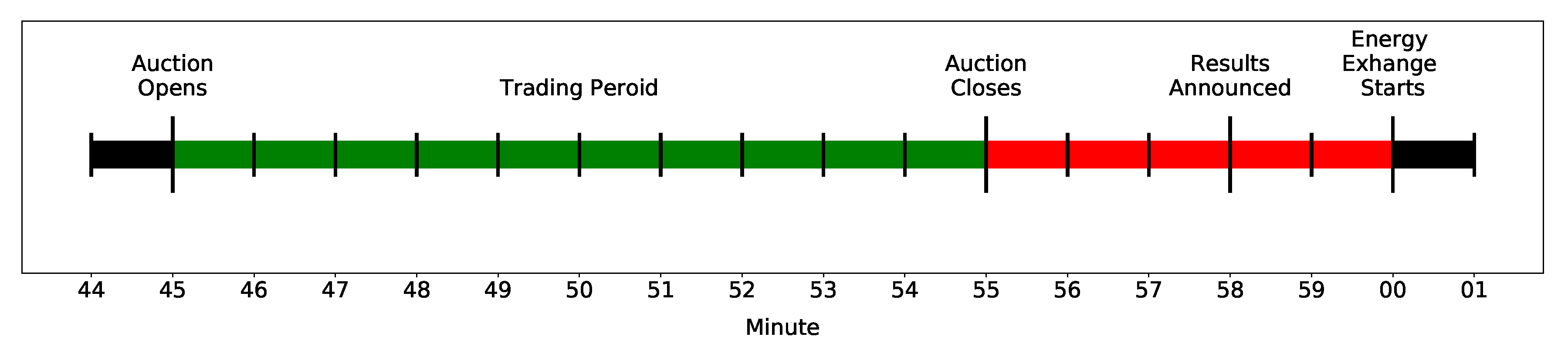
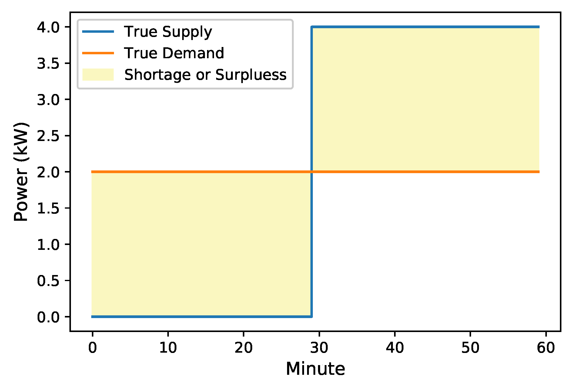
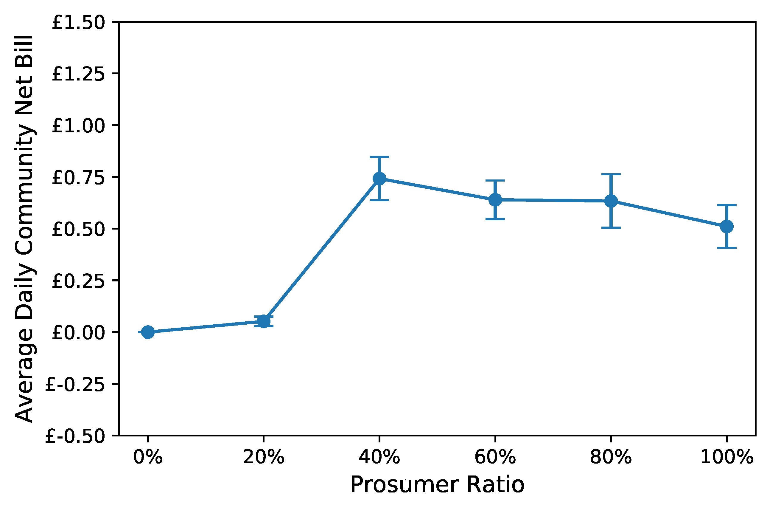
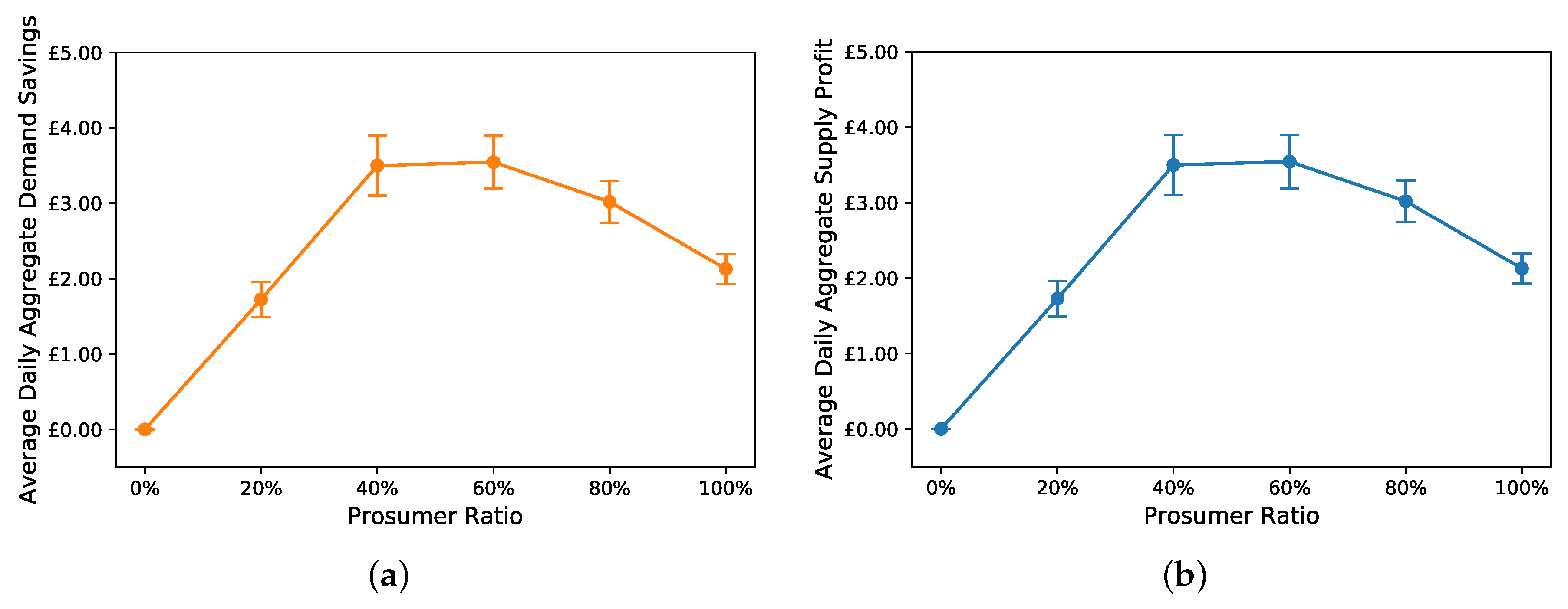
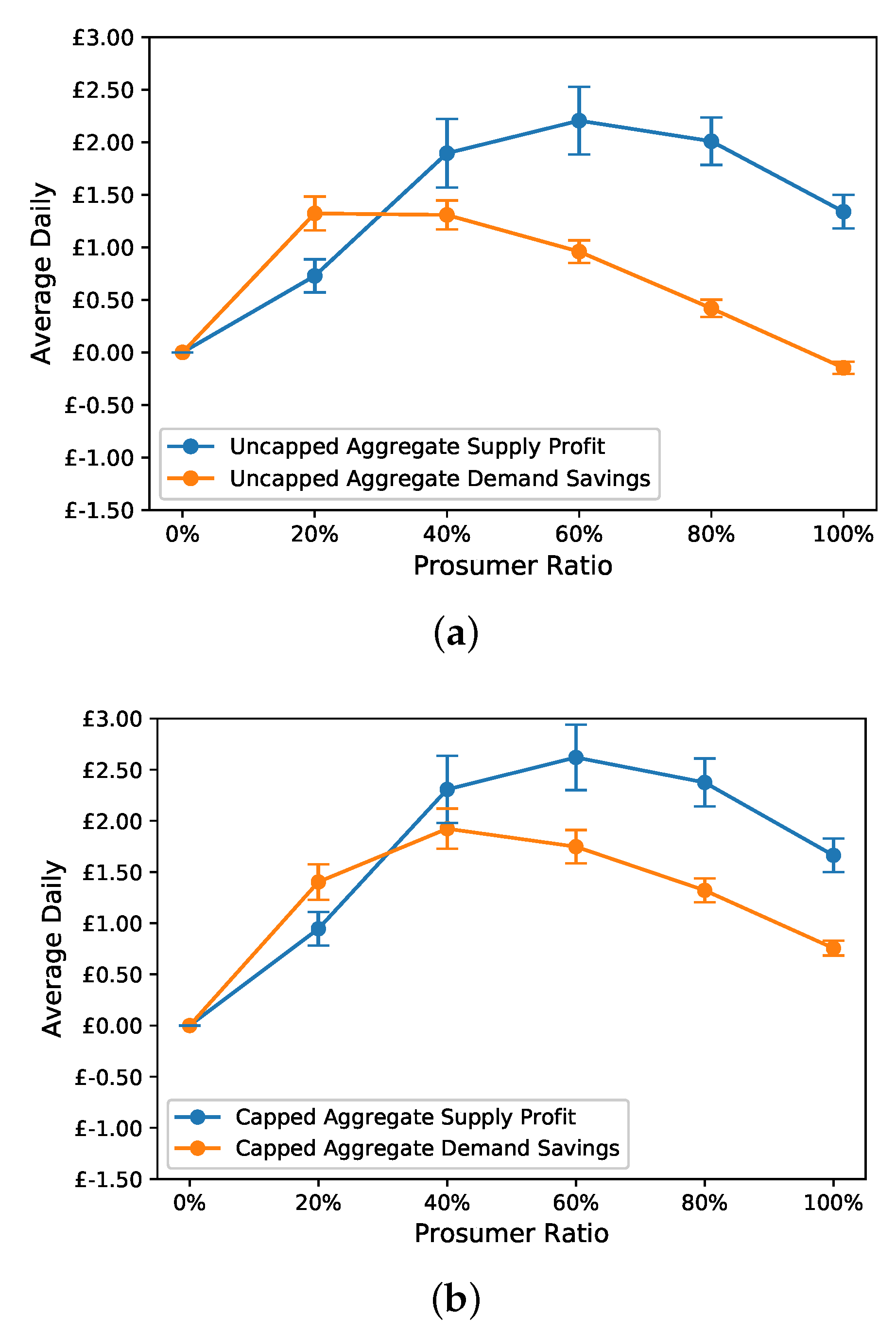
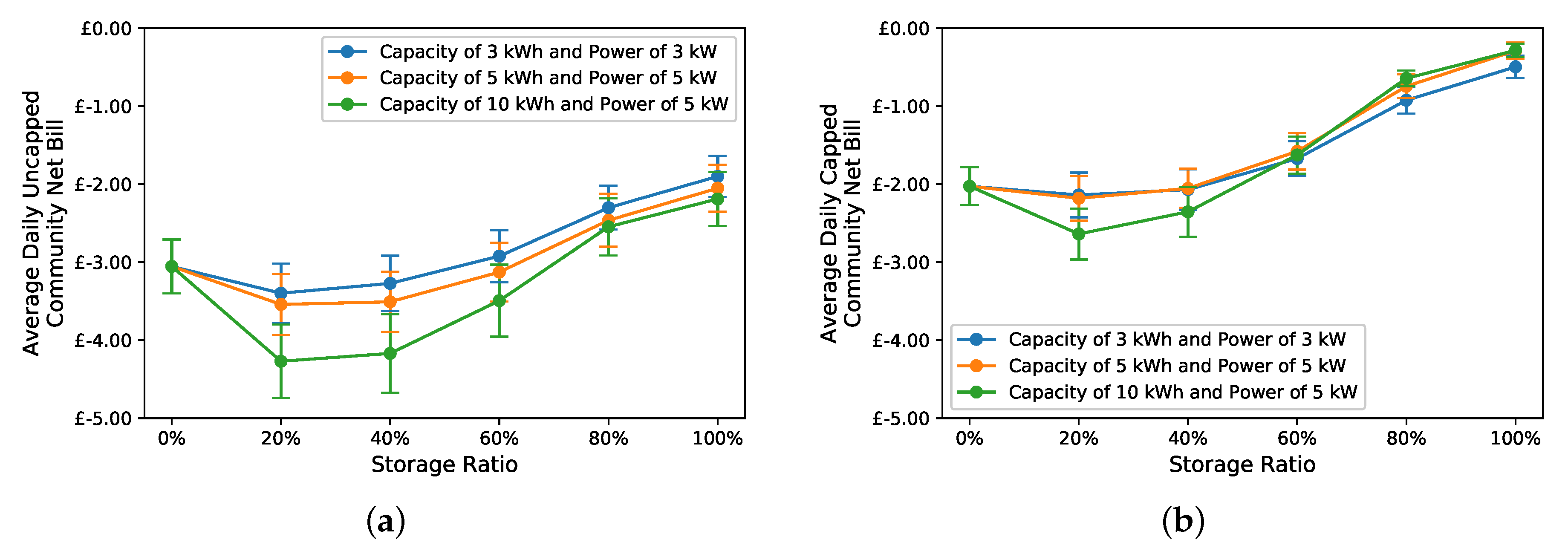
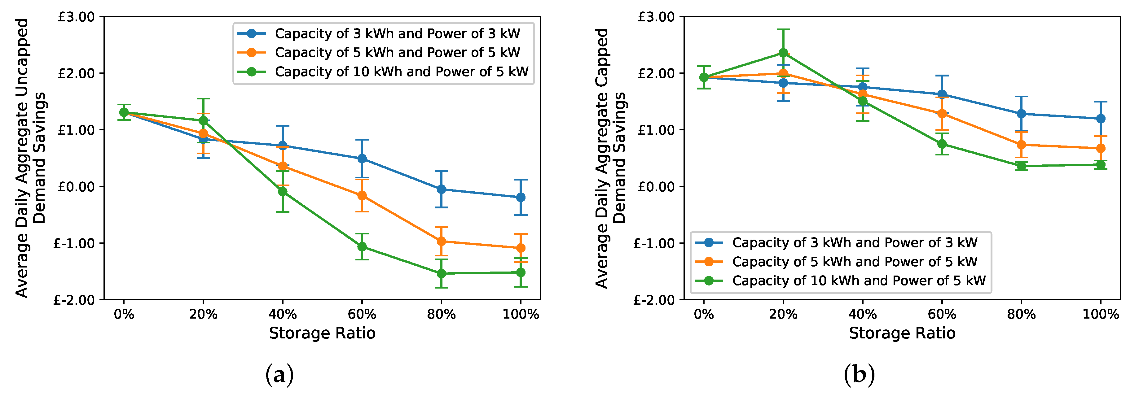
Table 1.
Simulations fixed parameters.
| Paramter | Value | Unit | Description |
|---|---|---|---|
| M | 29 | days | Length of the simulation |
| 1 | penny | Strategy price gap | |
| u | 1 | kWh | Strategy increment quantity |
| z | 0.5 | penny | Strategy price changing rate |
| y | 0.25 | penny | Strategy distance from the grid prices |
| 8.3 | pence | Buy price from the grid | |
| 3.41 | pence | Sell price to the grid |
Table 2.
The results for M in £ for the setting with perfect predictions without storage. At the end of the period, is in a deficit state with all prosumer ratios. and are highest with prosumer ratios between 40 and 60%.
Table 2.
The results for M in £ for the setting with perfect predictions without storage. At the end of the period, is in a deficit state with all prosumer ratios. and are highest with prosumer ratios between 40 and 60%.
| Prosumer Ratio | Aggregate Max PV Power | |||
|---|---|---|---|---|
| 20% | 20 | 1.51 | 50.05 | 50.05 |
| 40% | 50 | 21.51 | 101.51 | 101.51 |
| 60% | 85 | 18.54 | 102.82 | 102.82 |
| 80% | 125 | 18.38 | 87.54 | 87.54 |
| 100% | 185 | 14.80 | 61.71 | 61.71 |
Table 3.
The results for M in £ for the setting with perfect predictions with storage. At the end of the period, is in a deficit state in all storage ratio variations. However, increasing the storage ratio decreases the deficit. Also, increasing the storage ratio increases as more prosumers become flexible, but, it also reduces . By aggregating and , the configuration of 40% of prosumers having 10 kWh capacity storage devices, results in the most substantial combined benefit with 77% for .
| Ratio of Prosumers with Storage | Storage Capacity (kWh) | Storage Power (kW) | + | Aggregate Demand Savings From Storage Only | ||||
|---|---|---|---|---|---|---|---|---|
| 0% | 0 | 0 | 21.51 | 101.51 | 101.51 | 203.02 | 50% | |
| 20% | 3 | 3 | 17.70 | 95.71 | 141.10 | 236.81 | 60% | 18.66 |
| 40% | 3 | 3 | 15.13 | 82.65 | 170.18 | 252.83 | 67% | 39.66 |
| 60% | 3 | 3 | 13.64 | 68.63 | 190.65 | 259.28 | 74% | 61.32 |
| 80% | 3 | 3 | 10.77 | 48.64 | 214.18 | 262.82 | 81% | 82.94 |
| 100% | 3 | 3 | 9.10 | 39.00 | 225.78 | 264.78 | 85% | 102.73 |
| 20% | 5 | 5 | 18.32 | 100.43 | 149.25 | 249.68 | 60% | 22.43 |
| 40% | 5 | 5 | 14.24 | 78.55 | 190.64 | 269.19 | 71% | 47.35 |
| 60% | 5 | 5 | 11.19 | 52.04 | 221.85 | 273.89 | 81% | 74.48 |
| 80% | 5 | 5 | 10.27 | 27.30 | 237.68 | 264.98 | 90% | 101.82 |
| 100% | 5 | 5 | 7.07 | 23.00 | 244.41 | 267.41 | 91% | 125.41 |
| 20% | 10 | 5 | 13.04 | 111.32 | 174.30 | 285.62 | 61% | 25.17 |
| 40% | 10 | 5 | 8.54 | 69.53 | 232.86 | 302.39 | 77% | 52.79 |
| 60% | 10 | 5 | 8.77 | 31.95 | 252.88 | 284.83 | 89% | 84.96 |
| 80% | 10 | 5 | 10.40 | 15.89 | 241.31 | 257.20 | 94% | 117.50 |
| 100% | 10 | 5 | 5.54 | 15.62 | 251.00 | 266.62 | 94% | 144.44 |
Table 4.
Comparison between capped and uncapped results for the setting with imperfect predictions without storage for M in £. At the end of the period, both and are in surplus states. However, under the uncapped approach, increasing the prosumer ratio decreases until it becomes negative with 100% prosumers, whereas the capped approach maintains community surplus, and results in higher and .
| Prosumer Ratio | ||||||
|---|---|---|---|---|---|---|
| 20% | −39.11 | −30.47 | 38.36 | 40.70 | 21.12 | 27.42 |
| 40% | −88.60 | −58.81 | 37.94 | 55.78 | 54.97 | 66.92 |
| 60% | −95.30 | −60.42 | 27.83 | 50.69 | 63.97 | 75.98 |
| 80% | −86.25 | −49.51 | 12.17 | 38.31 | 58.29 | 68.88 |
| 100% | −74.05 | −38.48 | −4.26 | 21.91 | 38.83 | 48.23 |
Table 5.
Comparison between capped and uncapped results for the setting with imperfect predictions with storage for M in £. Both and are in a surplus states. However, increasing the storage ratio or the capacity decreases until it becomes negative. The capped approach maintains a community surplus and results in higher and . The ratio of in the benefits sum increase from 54% without storage to 66–96% with storage.
| Storage Ratio | Capacity (kWh) | Power (kW) | |||||||
|---|---|---|---|---|---|---|---|---|---|
| 0% | 0 | 0 | −88.60 | −58.81 | 37.94 | 55.78 | 54.97 | 66.92 | 54% |
| 20% | 3 | 3 | −98.55 | −62.05 | 24.17 | 52.94 | 96.05 | 103.78 | 66% |
| 40% | 3 | 3 | −94.90 | −60.05 | 20.89 | 50.85 | 123.77 | 128.66 | 72% |
| 60% | 3 | 3 | −84.77 | −48.50 | 14.22 | 47.15 | 151.31 | 154.65 | 77% |
| 80% | 3 | 3 | −66.78 | −26.85 | −1.49 | 37.15 | 187.65 | 188.94 | 84% |
| 100% | 3 | 3 | −55.13 | −14.45 | −5.59 | 34.68 | 211.92 | 212.33 | 86% |
| 20% | 5 | 5 | −102.72 | −63.27 | 27.10 | 57.81 | 99.19 | 107.93 | 65% |
| 40% | 5 | 5 | −101.75 | −59.59 | 10.38 | 47.13 | 142.06 | 147.46 | 76% |
| 60% | 5 | 5 | −90.71 | −45.83 | −4.69 | 37.27 | 178.73 | 181.65 | 83% |
| 80% | 5 | 5 | −71.47 | −21.66 | −28.10 | 21.31 | 218.65 | 219.06 | 91% |
| 100% | 5 | 5 | −59.52 | −8.42 | −31.54 | 19.47 | 241.28 | 241.38 | 93% |
| 20% | 10 | 5 | −123.84 | −76.54 | 33.65 | 68.33 | 108.44 | 121.07 | 64% |
| 40% | 10 | 5 | −120.92 | −68.30 | −2.65 | 43.67 | 170.85 | 177.16 | 80% |
| 60% | 10 | 5 | −101.32 | −47.18 | −30.85 | 21.70 | 213.13 | 214.73 | 91% |
| 80% | 10 | 5 | −73.88 | −18.71 | −44.61 | 10.39 | 227.04 | 227.22 | 96% |
| 100% | 10 | 5 | −63.52 | −8.30 | −44.00 | 11.13 | 249.15 | 249.24 | 96% |
© 2020 by the authors. Licensee MDPI, Basel, Switzerland. This article is an open access article distributed under the terms and conditions of the Creative Commons Attribution (CC BY) license (http://creativecommons.org/licenses/by/4.0/).
Share and Cite
MDPI and ACS Style
Alabdullatif, A.M.; Gerding, E.H.; Perez-Diaz, A. Market Design and Trading Strategies for Community Energy Markets with Storage and Renewable Supply. Energies 2020, 13, 972. https://doi.org/10.3390/en13040972
AMA Style
Alabdullatif AM, Gerding EH, Perez-Diaz A. Market Design and Trading Strategies for Community Energy Markets with Storage and Renewable Supply. Energies. 2020; 13(4):972. https://doi.org/10.3390/en13040972
Chicago/Turabian StyleAlabdullatif, Abdullah M., Enrico H. Gerding, and Alvaro Perez-Diaz. 2020. "Market Design and Trading Strategies for Community Energy Markets with Storage and Renewable Supply" Energies 13, no. 4: 972. https://doi.org/10.3390/en13040972
Note that from the first issue of 2016, this journal uses article numbers instead of page numbers. See further details here.