Modelling Heat Pumps with Variable EER and COP in EnergyPlus: A Case Study Applied to Ground Source and Heat Recovery Heat Pump Systems


DIME, University of Genova, Via all’Opera Pia 15a, 16145 Genova, Italy
*
Author to whom correspondence should be addressed.
Energies 2020, 13(4), 794; https://doi.org/10.3390/en13040794
Submission received: 3 December 2019
/
Revised: 28 January 2020
/
Accepted: 5 February 2020
/
Published: 11 February 2020
(This article belongs to the Special Issue Design of Heat Exchangers for Heat Pump Applications)
Abstract
:Dynamic energy modelling of buildings is a key factor for developing new strategies for energy management and consumption reduction. For this reason, the EnergyPlus software was used to model a near-zero energy building (Smart Energy Buildings, SEB) located in Savona, Italy. In particular, the focus of the present paper concerns the modeling of the ground source water-to-water heat pump (WHP) and the air-to-air heat pump (AHP) installed in the SEB building. To model the WHP in EnergyPlus, the Curve Fit Method was selected. Starting from manufacturer data, this model allows to estimate the COP of the HP for different temperature working conditions. The procedure was extended to the AHP. This unit is a part of the air-handling unit and it is working as a heat recovery system. The results obtained show that the HP performance in EnergyPlus can closely follow manufacturer data if proper input recasting is performed for EnergyPlus simulations. The present paper clarifies a long series of missed information on EnergyPlus reference sources and allows the huge amount of EnergyPlus users to properly and consciously run simulations, especially when unconventional heat pumps are present.
1. Introduction
Energy savings and emissions reduction are two major keywords in the worldwide research scenario. One of the main responsible sectors is the buildings one, with approximately 40% of energy consumption and 36% of CO2 emissions in the EU [1]. In this framework, it is easy to understand why energy dynamic simulations of buildings are of great importance and can be used to either develop innovative solutions for new buildings or to evaluate different retrofit interventions to enhance the energy performance of existing ones [2,3,4].
To decrease energy consumption and pollutant emissions, the first mandatory step is the reduction of building loads (i.e., building energy needs) by means of actions on the building envelope and related to the building operating conditions [5]. These include techniques to increase the external insulation combined with actions for the exploitation of the solar gains to reduce heating loads during winter [6].
After the activities devoted to minimizing the energy needs of the building, the second step is to select and correctly size innovative plants for heating and cooling that, if possible, include the use of renewable energies.
For example, solar energy can be exploited in thermal solar collectors to produce Domestic Hot Water (DHW) and in photovoltaic (PV) fields for powering the air conditioning system of buildings [7]. In particular, during the summer season, periods with higher solar radiation coincide with higher electrical energy demand for the cooling air conditioning systems and the use of PV modules helps to reduce the electrical national grid stress.
In recent years, one of the more frequently selected plant solutions for air conditioning in buildings has included reversible heat pumps (HPs) that allow to satisfy building requests both in heating and in cooling. Among them, Ground Coupled Heat Pumps (GCHP) are a very effective configuration, exploiting the near constant ground temperature during the year to increase the performance coefficients (EER in cooling mode and COP in heating mode) [8,9,10]. Performance of the ground-coupled heat pump greatly depends on several factors, including the fluid temperatures, the ground thermophysical properties and the configuration of Borehole Heat Exchangers (BHEs) used in the installation [11].
Another interesting plant solution is air-to-air heat pumps devoted to heat recovery on ventilation. This type of systems can be simple (i.e., direct expansion, DX) for the air conditioning of a single zone of a building, or more complex and sophisticated (i.e., included in air-handling unit, AHU), used for ventilation, humidification, filtration and air-conditioning with energy recovery (both active and passive techniques) of entire buildings.
It is apparent that one of the main problems in the correct sizing and in the modelling process of a heat pump is to take properly into account the variation of its performance in different operating conditions. In fact, the COP of a heat pump, even at full load, changes at different condensations and evaporation temperatures, which depend on the source and load side temperatures. For technological innovative solutions, the modelling process to include the heat pump in energy dynamic simulations can be difficult.
Lee et al. [12] recently developed a simplified heat exchanger model using artificial neural networks. Using a genetic algorithm, they managed to optimize the operating and design parameters of the heat exchanger in order to maximize the seasonal EER and the seasonal COP with respect to the outdoor temperature. Torregrosa-Jaime et al. [13] modelled the performances of a Variable Refrigerant Flow (VRF) equipment. They analysed the model proposed in EnergyPlus and they developed a new one using a BIM approach. Finally, they compared the results obtained with the manufacturer data.
Models for heat pumps pertain to two main groups, with two different approaches to the problem [14]. On one hand, there are the “equation fit models”, which consider the heat pump as a black box, whose behavior is simulated by means of correlations with coefficients derived from manufacturer data. On the other hand, there are “deterministic models” that consider each component of the system applying energy and mass conservation equations.
The main differences between the two approaches are the amount of data requested and the application aim. The equation fit models are easier because they need only the knowledge of the performance at the operating conditions usually given by the manufacturer [15,16]. On the contrary, deterministic models also need data for specific HP components: these parameters often derive from dedicated measurement campaigns and are not provided by the manufacturer. This approach is useful for the study and design of specific components of the heat pump.
In dynamic simulations over long periods (e.g., yearly simulations for building response to environmental conditions and internal energy transfers), the working conditions of a heat pump change continuously, and it is mandatory to include, inside the model, at least the COP variation with temperature. The starting point are the data provided by the manufacturer in terms of the performance coefficients of the heat pump in heating and cooling at reference working conditions.
This paper deals with HP modelling in EnergyPlus environment. The application of the “equation fit model” is applied for modelling a water-to-water heat hump (Curve Fit Method [17]) and an air-to-air heat pump [18], the latter being applied for heat recovery purposes on air ventilation circuit.
To the above aim, a case study was taken into account and it refers to a n-ZEB building located at the Savona Campus of the University of Genova, Italy. In this case, a water-to-water heat pump is coupled with the ground and fed by water circulating in a borehole heat exchangers (BHEs) field. If the ground heat transfer is correctly evaluated, the returning fluid temperature (from the boreholes to the heat pump) is known with good approximation. The load side water temperature is imposed, based on the building request and on the operating condition of the distribution system (for the analyzed case composed by fancoils and radiators).
The investigated air-to-air heat pump is included in an air-handling unit and it serves as an energy recovery system on the exhaust air from ventilation. Thus, for that special air-to-air heat pump, the load side temperature is the external one, whereas the source side temperature is the return temperature from the building, nearly stable in both cooling and heating conditions.
By means of EnergyPlus simulations using “equation fit models”, the variables EER and COP of both the heat pumps were evaluated for selected couples of source side and load side temperatures. For the water-to-water heat pump, the effect of the water volumetric flow rates (source and load side) was also taken into account by employing the manufacturer data related to the partial load factor (PLF) effect. For the air-to-air heat pump, the original contribution of the present study is the analysis of the suitable input datasets in case of unconventional heat pumps like the one with energy recovery here considered.
The good agreement between expected results and simulations validates the analysis. The present paper is in addition clarifying a long series of missed information on Energy Plus reference sources in order to allow the huge amount of Energy Plus users to efficiently, properly and consciously run simulations when considering temperature varying COPs.
2. Water-to-Water Heat Pump Model
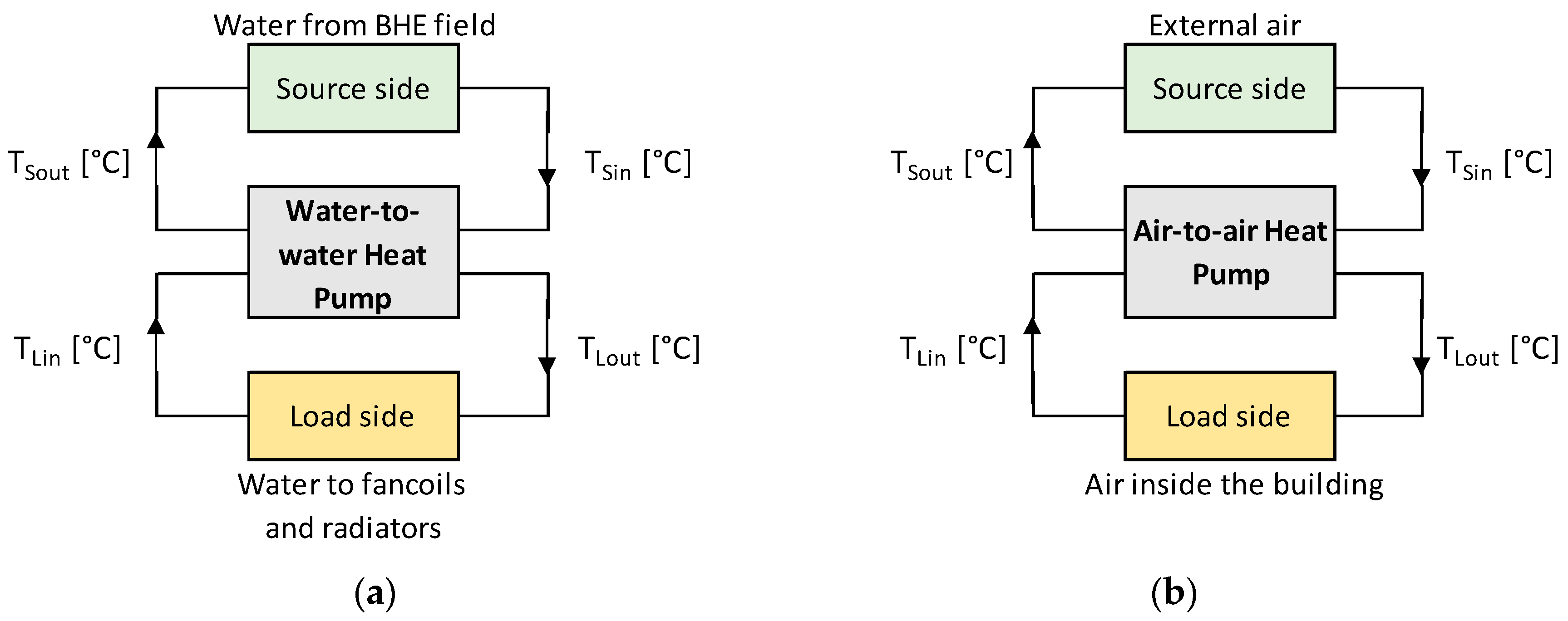
This paragraph presents the literature models selected in the present study in order to properly address the input in the Energy Plus program to simulate water-to-water and air-to-air heat pumps (Figure 1) at temperature varying COP. The detailed description provided (and the related validations) here are original contributions of the present study, since Energy Plus references do not fully specify how the code can properly manage the running mode when inverse machines performance have to be customized in terms of manufacturer information.
In EnergyPlus, two different options are available to model the water-to-water heat pumps, i.e., the “Curve Fit Method” and the “Parameter estimation-based model” [15].
For the case study reported in this paper, the selected model is the “Curve Fit Method”, which allows quicker simulation of the water-to-water heat pump, avoiding the drawbacks associated with the more computationally expensive “Parameter estimation-based model”.
The variables that influence the water-to-water heat pump performance are mainly inlet water temperatures (source and load side) and water volumetric flow rates (source and load side).
The governing equations of the “Curve Fit Method” for the cooling and heating mode are the following ones [16]:
Cooling Mode:
Heating Mode:
where the parameters are defined as:
| Ai, Bi, Di, Ei | Equation fit coefficients for the cooling and heating mode [-]. |
| Tref | Reference temperature, 283.15 [K]. |
| TL,in | Load side inlet (in the HP) water temperature, [K]. |
| TS,in | Source side inlet (in the HP) water temperature, [K]. |
| Load side volumetric flow rate [m3/s]. | |
| Source side volumetric flow rate [m3/s]. | |
| Load side heat transfer rate (cooling/heating mode) [W]. | |
| Power consumption (cooling/heating mode) [W]. |
The subscript “ref” indicates values at reference conditions that must be correctly specified. The reference temperature is always equal to 10 °C (283.15 K) and even when available data from manufacturer are provided at a different values, performance is to be recast to the above temperature.
In cooling mode, the reference conditions are when the heat pump operates at the highest (nominal) cooling capacity indicated in the manufacturer’s technical references. The above condition does not match the real heat pump/chiller behavior since its performance can be even better than those at the nominal capacity, provided that the working temperature are “better” than the performance test ones. Similarly, in heating mode, the reference conditions are when the heat pump is operating at the highest (nominal) heating capacity.
In EnergyPlus, when selecting the “Curve Fit Method” to model water-to-water heat pumps, one must specify the parameters at the reference conditions and provide the equation fit coefficients.
Once the type of the water-to-water heat pump is selected, the generalized least square method is used for the evaluation of the coefficients Ai, Bi, Di, Ei, based on the data available from the manufacturer’s catalogue.
The performance coefficients (EER in cooling mode and COP in heating mode) are evaluated as the ratio between the useful heat transfer rate (load side) (Equations (1) and (3)) and the related power consumption (Equations (2) and (4)). Their equations as function of inlet temperatures and volumetric flow rates are, respectively:
Cooling Mode:
Heating Mode:
3. Air-to-Air Heat Pump Model
Air-to-air heat pump is here again modelled with an “equation fit model” [18].
Assuming constant supply air volumetric flow rate as operating conditions, the cooling and heating capacities and the EER and COP (and EIR = 1/EER) are only depending on temperatures and the selected equations to model the air-to-air heat pump are biquadratic ones. In particular, the performance depends on the “load air wet-bulb temperature” TL,in wb and the “source air dry-bulb temperature” TS,in db in cooling mode and on the “load air dry-bulb temperature” TL,in db and the “source air dry-bulb temperature” TS,in db in heating mode.
Cooling Mode:
Heating Mode:
In the previous equations, the parameters are defined as:
| Load side heat transfer rate (cooling/heating mode) [W]. | |
| EER | Overall efficiency in cooling mode (thermodynamic circuit and fans) [-]. |
| EIR | Performance coefficient in cooling mode (=1/EER) [-]. |
| COP | Overall efficiency in heating mode (thermodynamic circuit and fans) [-]. |
| ai, bi, ci, di | Equation fit coefficients for the cooling and heating mode [-]. |
| TL,in wb | Load side inlet (in the HP) air wet bulb temperature, [K]. |
| TL,in db | Load side inlet (in the HP) air dry bulb temperature, [K]. |
| TS,in db | Source side air inlet (in the HP) dry bulb temperature, [K]. |
The subscript “ref” indicates values at reference conditions that must be correctly specified.
In EnergyPlus the reference conditions are required both in cooling and in heating mode. For the standard operating condition, in cooling mode, the reference load side air wet-bulb temperature TL,in wb ref is equal to 19.4 °C (with a corresponding reference load side air dry-bulb temperature TL,in db ref equal to 26.7 °C) whereas the source side air dry-bulb temperature is fixed at 35 °C. In heating mode, the reference load side air dry-bulb temperature TL,in wb ref is equal to 21.1 °C, whereas the source side air dry-bulb temperature is fixed at 8.3 °C.
In fact, for conventional reversible heat pumps, the load side conditions correspond to internal building ones (return air temperature TRA) whereas source side conditions correspond to external ones (external air temperature TOA).
4. The Case Study: The Smart Energy Building (SEB)
The Smart Energy Building (SEB) was conceived and built by the University of Genoa (Unige) as an innovative and high-performance building to meet goals of zero carbon emissions, energy and water efficiency and building automation. It is located in the Unige Campus of Savona, Italy.
The two storey building, in operation since February 2017, has a total floor area of about 1000 m2. In particular, SEB is characterized by the presence of:
- high-performance thermal insulation materials for the envelope;
- ventilated facades;
- a photovoltaic field (21 kWp) on the roof;
- extremely low consumption led lamps;
- a rainwater collection system;
- a thermal system composed by:
- ✓
- an air handling unit (AHU), associated to an air-to-air heat pump, installed on the roof, which performs functions such as circulating, cleaning and cooling/heating the air of the building;
- ✓
- a ground coupled heat pump (GCHP), that produces cold/hot water to feed fancoils and radiators for cooling/heating purpose; the hot water is used during winter also for Domestic Hot Water (DHW) purposes;
- ✓
- two solar thermal collectors, for DHW production purposes exclusively;
- ✓
- an air source heat pump (ASHP), for DHW production as backup unit of the solar collectors.
The innovative nature of this building suggests the opportunity to analyze its performance from a dynamic point of view and to develop an energy model suitable for hourly simulations. EnergyPlus was selected to this aim. In particular, the present paper is focused on the modeling of the water-to-water ground coupled heat pump (GCHP) and on the air-to air heat pump associated to the AHU.
4.1. Modelling the Water-to-Water Ground Coupled Heat Pump (GCHP)
For the Smart Energy Building, the geothermal heat pump in operation is a Clivet brand, model WSHN-XEE2 MF 14.2, operating with brine (geothermal side) and water. In particular, data refer to operation with a mixture of water and propylene glycol at 30% on the source side.
The manufacturer catalogue provides the heat pump performance at full load as a function of source/load fluid temperatures. Table 1 represents the manufacturer data for the size 14.2, for the cooling mode.
The performance at full load related to the heating operating mode as a function of temperatures are provided by the Manufacturer in two different Tables depending on the range of the source side water temperature. For our test case, it is interesting to consider a wide range of working conditions for the source side temperature. In fact, for a GCHP with expected long life of operation, the temperature of the ground, starting from the undisturbed value, can change considerably in time [19] and consequently, the temperature of the fluid circulating in the BHE field changes.
The two manufacturer tables for heating mode differ for the selected values of the load side temperatures and thus, it is necessary to apply a proper interpolations. This is a typical problem in manufacturer data and cannot be managed in Energy Plus in a different way. The obtained combined dataset for heating mode is presented in Table 2. In grey are the data achieved by interpolation.
It is important to notice that the performances in Table 1 and Table 2 are provided as a function of the outlet temperatures TS,out and TL,out whereas Equations (11)–(16) contain the inlet ones, TS,in and TL,in.
However, the manufacture catalogue provides details about the operating conditions related to the performances of Table 1 and Table 2. In detail, the EER and COP data refer to following imposed temperature difference at the load and source sides:
Cooling (Table 1):
Heating (Table 2):
For a complete analysis, it is necessary to take into account also the effect of water volumetric flow rates (source and load side) on the heat pump performance. The manufacturer provides only little information about the effect of the partial load factor PLF on the EER and COP of the water-to-water heat pump and in particular the performance at PLF of 67% and 33%. Both the EER and the COP are enhanced at partial load, according to Table 3.
Considering that both the source and load sides of the HP work at constant temperature difference according to Equations (11) and (12), the PLF represents not only the ratio between actual cooling or heating capacity and the maximum value but also the corresponding ratio between the water volumetric flow rates at load side. From the values of EER or COP in Table 3 it is possible to deduce the power consumption (cooling and heating mode) and the source side heat transfer rate and, as a consequence, the water volumetric flow rates at source side.
The coefficients Ai, Bi, Di and Ei of Equations (1)–(6) are not available from manufacturer references. The only way for accessing them is to iteratively guess their correct value by comparison with the available datasheet values and by minimizing an error. In this paper, a simple optimum search process was applied to cooling or heating capacity and power consumption values provided in the manufacturer catalogue.
The final calculated coefficients are presented in Table 4.
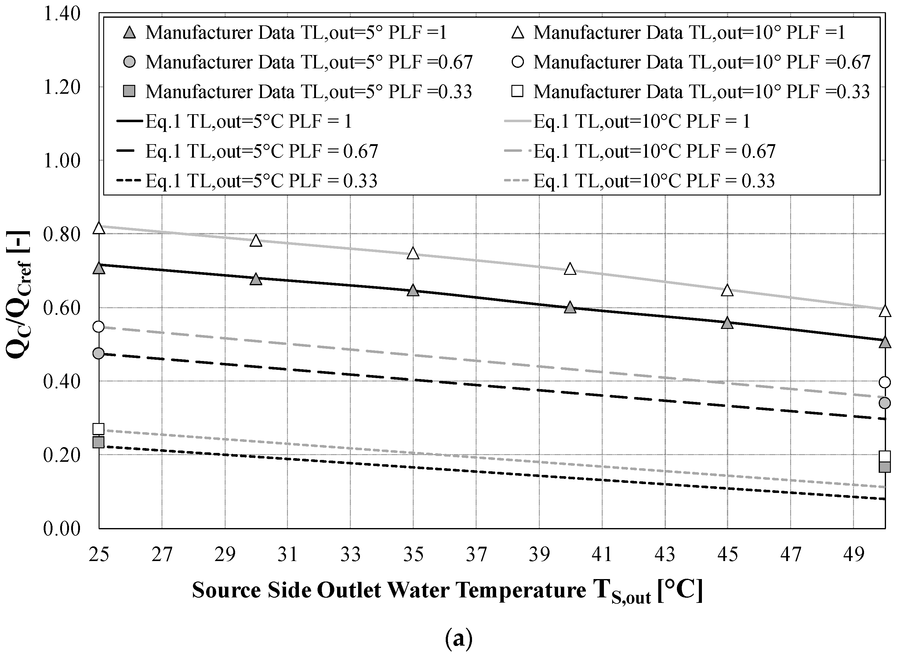
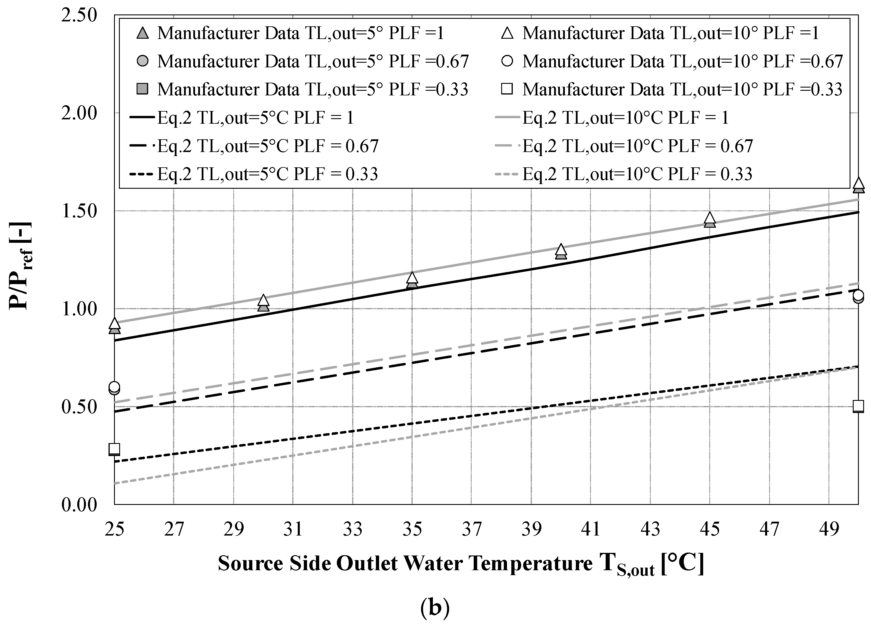
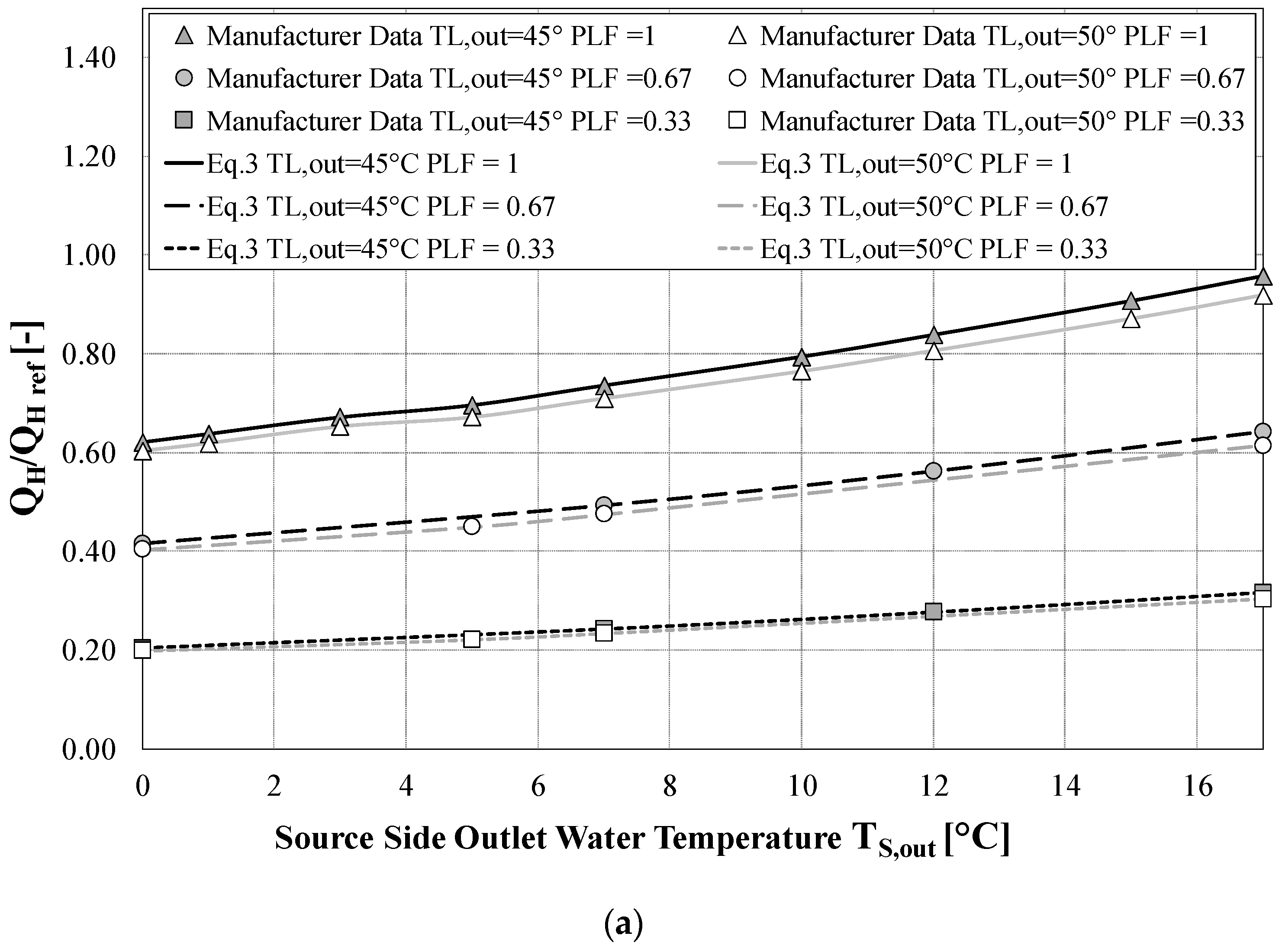
Figure 2 and Figure 3 compare the manufacturer data with the values obtained with the correlations 1–4 using the optimum calculated coefficients of Table 4. In particular, the graphs show the cooling/heating capacities and the power consumptions for cooling and heating, respectively, as a function of the source side outlet water temperature TS,out with the load side outlet water temperature TL,out as a parameter and considering the three conditions of load, namely PLF = 1, 0.67, 0.33.
During the summer season, the cooling capacity decreases to increase the source side outlet water temperature TS,out (fluid temperature entering in the BHE field) and increases to increase the load side outlet water temperature TL,out (fluid temperature to fancoils and radiators). On the contrary, the power consumption P increases to increase the source side outlet water temperature TS,out whereas the effect of the load side outlet water temperature TL,out is nearly negligible. As expected, both the cooling capacity and the power consumption decreased by decreasing the partial load factor PLF.
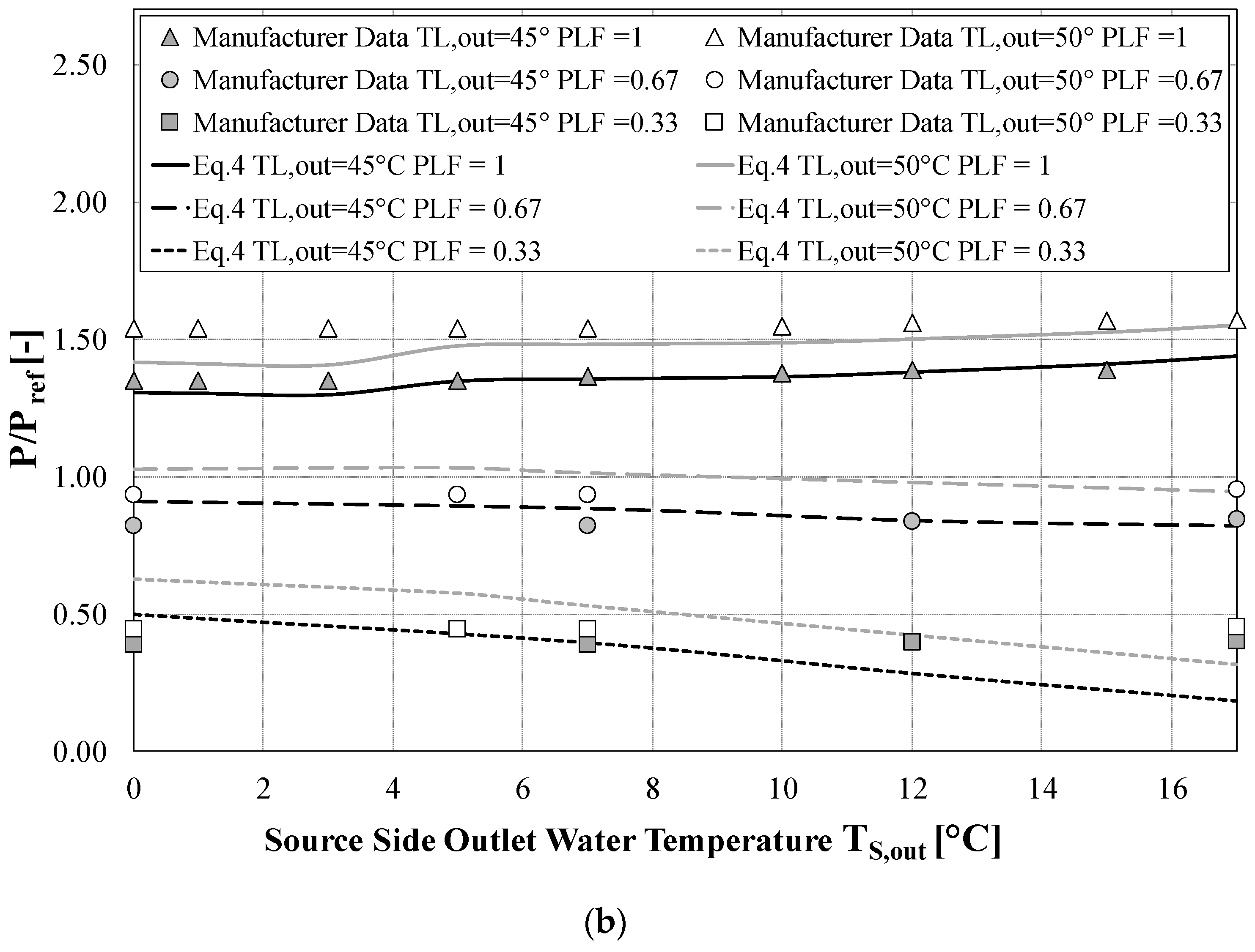
During winter, on the other hand, the heating capacity increases for increasing source side outlet water temperature TS,out and slightly decreases for increasing load side outlet water temperature TL,out. The power consumption P is marginally affected by the source side outlet water temperature TS,out, whereas it increases with the load side outlet water temperature TL,out.
The particular trend of the curve given by Equations (3) and (4), with two slight inflection points for TS,out = 3 and 5 °C, is due to the particular operating conditions for the manufacture catalogue in heating mode. In fact, manufacture tables in the heating mode are built for different imposed temperature differences at the load and source sides, according to Equation (12). Thus, at different source sides, “outlet” water temperatures TS,out correspond the same source side “inlet” water temperatures TS,in = 8 °C that represents the input of Equations (3) and (4).
As for the cooling case, both the heating capacity and the power consumption decrease by decreasing the partial load factor PLF.
The agreement between manufacture dataset and “equation fit models” approach is good, with an average relative error between less than 7%, for both cooling and heating mode at full load and lower than 15% considering also the PLF = 0.67 and 0.33.
4.2. Modelling the Air-to-Air Heat Pump
For the Smart Energy Building, the selected air-to-air heat pump associated to the air handling unit (AHU) is the Clivet Zephir CPAN-XHE3 Size 3, with a standard air flow of 4600 m3/h. This volumetric flow rate fulfils the ventilation requested by the Italian standards for the SEB building in terms of its volume and expected occupancy levels.
This air unit is very peculiar, especially if compared with the options conceived and available in Energy Plus. This system is a primary-air plant with a thermodynamic recovery of the energy contained in the return air. The primary air comes entirely from outdoor (fresh-air) at temperature TOA whereas the return-air comes from the building inner rooms at temperature TRA. Return air, before being released to the atmosphere, exchanges heat with the condenser in cooling mode and with the evaporator in heating mode. Return-air represents a favorable thermal source stable in time, offering lower temperature on the condenser side in cooling mode and higher temperature on the evaporator side in heating mode. As a consequent, the energy required by the compressors is reduced up to 50% [20].
The manufacturer catalogue provides the reversible heat pump performances as a function of external air temperature TOA (dry bulb/wet bulb) and supply air temperature TSA. Moreover, the manufacturer catalogue reports two different types of performance coefficients, the thermodynamic efficiencies (EERth and COPth) and the overall efficiencies (EER and COP) that consider also the power of the auxiliary systems.
In cooling mode, the selected supply humidity ratio is equal to 11 gvap/kgair and the reference return air temperature TRA is 26 °C. In heating mode, the reference return air temperature TRA is 20/12 °C (dry bulb/wet bulb). To model the air-to-air HP in EnergyPlus, the data corresponding to the “MC” operation mode were not considered, that imply post-heating equal to zero in cooling mode.
The distinctive operating conditions of the present heat pump (with energy recovery) allow it to reach high values of performance coefficients but create some challenges in modelling the system in EnergyPlus. In fact, the “load side” temperature becomes the external air temperature TOA whereas the “source side” temperature is the return air temperature TRA both in cooling and in heating modes. Consequently, the reference conditions suggested from EnergyPlus (Par. 2.2) are no longer valid and new reference conditions are defined for the analyzed present heat pump.
In particular, in cooling mode, the new reference external air temperature TOA is set to 40/25 °C (dry-bulb/wet-bulb) whereas the reference return air temperature TRA is set to 26 °C (Table 5). In heating mode, the new reference external air temperature TOA is set to −5 °C (dry-bulb) whereas the reference return air temperature TRA is set to 20/12 °C (dry bulb/wet bulb) (Table 6).
The EnergyPlus model for the air-to-air heat pump implements Equations (7)–(10) that express the cooling/heating capacities and the EIR, COP as a function of both the external air temperature TOA (dry-bulb/wet-bulb) and the return air temperature TRA. Unfortunately (again a typical case), the data provided by the manufacturer are a function of a unique value of the return temperature TRA, namely 26 °C in cooling and 20/12 °C (dry bulb/wet bulb) in heating.
Thus, it is necessary to create an extended database to obtain, by optimization, the coefficients ai, bi, ci and di of Equations (7)–(10). The selected return temperatures TRA to extend the dataset are 20, 22, 26 °C.
By keeping constant the air volumetric flow rate, for the same external and supply conditions (temperature and humidity), also the cooling and heating capacities remain constant. On the contrary, modifying the return temperature conditions changes the “source temperature” and as a consequence, the performance coefficients (EER and COP) and the compressor power are modified.
The values of the thermodynamic performance coefficients (EERth and COPth) for the new values of the return temperatures TRA are obtained by multiplying the corresponding Carnot performance coefficients (EERCarnot and COPCarnot) based on the evaporator and condenser temperatures, by two sets of constants CCi and CHi.
The coefficients CCi and CHi are calculated here from Carnot law and manufacturer data according to the expressions below. Moreover, they are assumed to be dependent on the supply air temperature TSA but independent of the return temperatures TRA.
The evaporator temperature Tevap is assumed to be nearly equal to the supply air temperature TSA whereas the condenser temperature Tcond is evaluated by means of energy balances on the components of the HP.
The condenser temperature Tcond is assumed to be nearly equal to the supply air temperature TSA whereas the evaporator temperature Tevap is evaluated by means of energy balances on the components of the HP.
Finally, overall efficiencies (EER and COP) are deduced by assuming the fan power consumption as constant and equal to 1 kW for all the operating conditions considered.
The results of this analysis are presented in Table 5 and Table 6, in cooling and heating mode respectively (data in grey, original data provided by the manufacturer in white).
Finally, by means of an optimum search process comparing the performance values of Table 5 and Table 6, the coefficients ai, bi, ci and di of Equations (7)–(10) were obtained and the results are presented in Table 7.
As an example, Figure 4 and Figure 5 show the cooling and heating capacities and the HP performances (EIR and COP) as a function of external conditions TOA and return temperature TRA as parameter. In particular, the manufactured data reported in Table 5 and Table 6 are compared with the curves obtained by using Equations (7)–(10) with the least square error coefficients of Table 7.
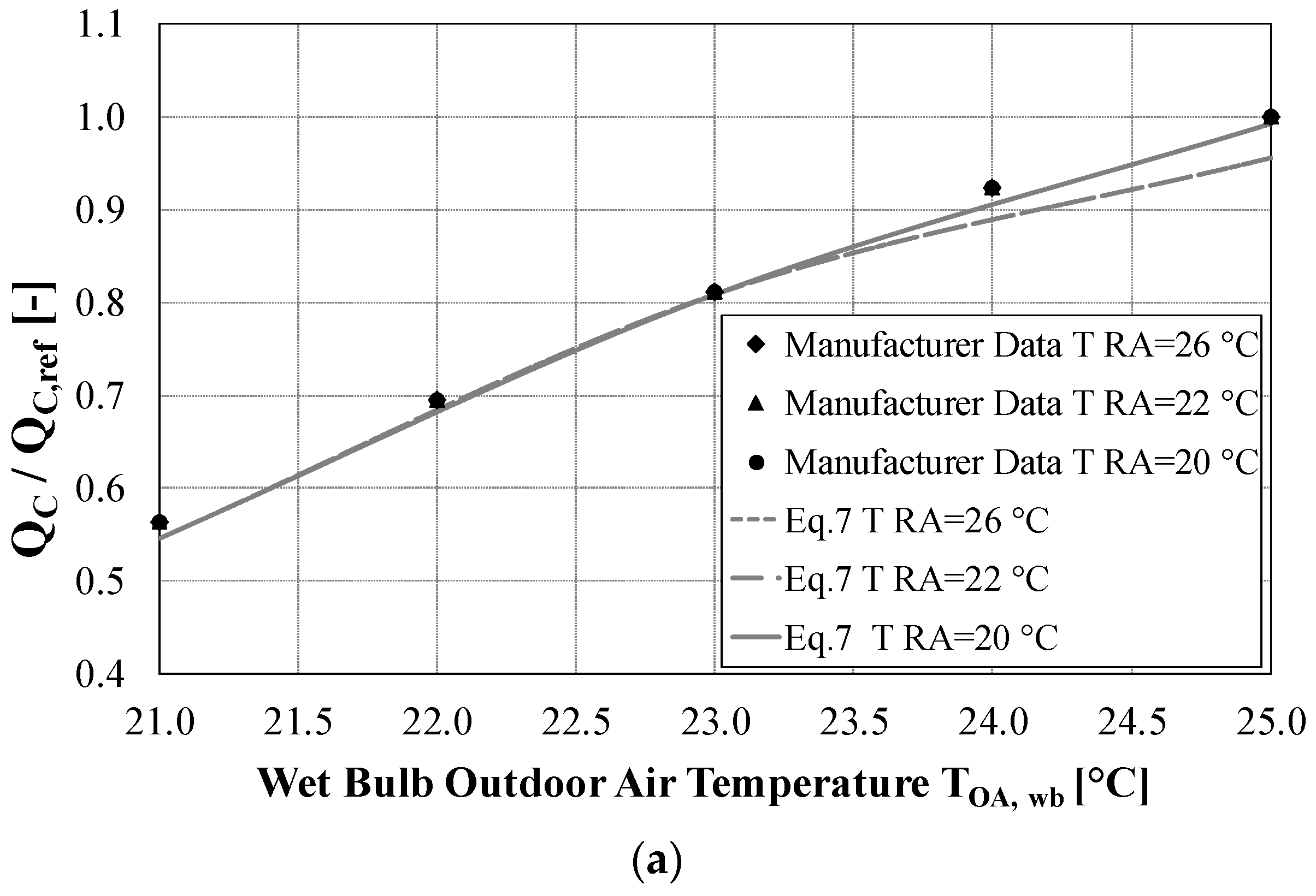
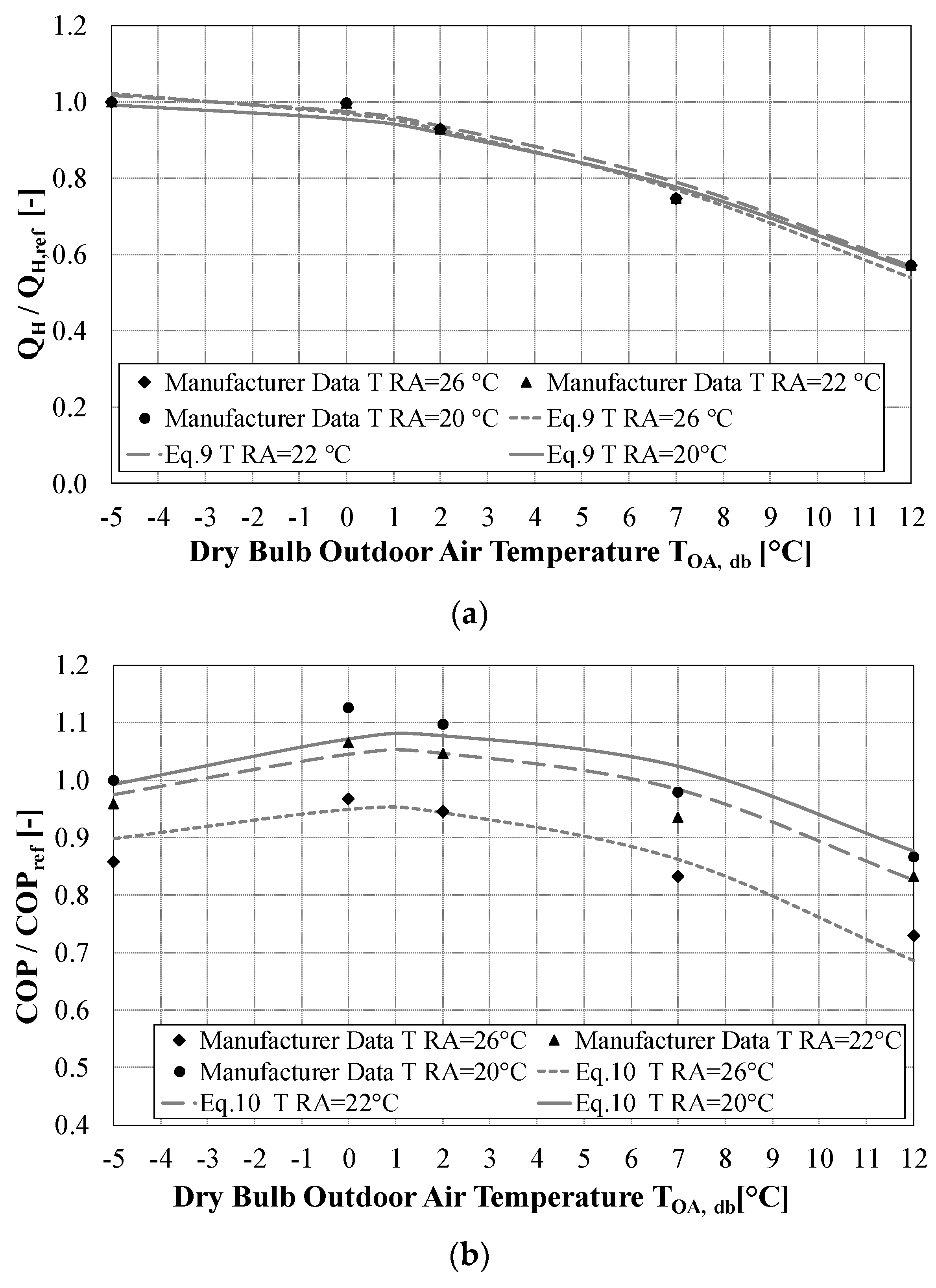
As expected, not changing the volumetric flow rate and the external TOA and supply conditions (temperature and humidity), the cooling and heating capacities remain almost constant for the different return air conditions TRA (Figure 4a and Figure 5a). The cooling capacity (requested by the building) increases with the external temperature TOA whereas the heating capacity (requested by the building) decreases by increasing the external temperature TOA.
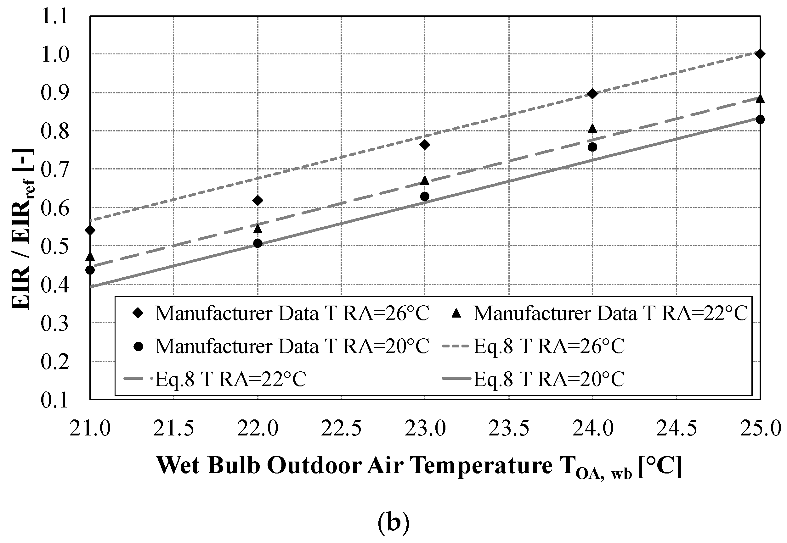
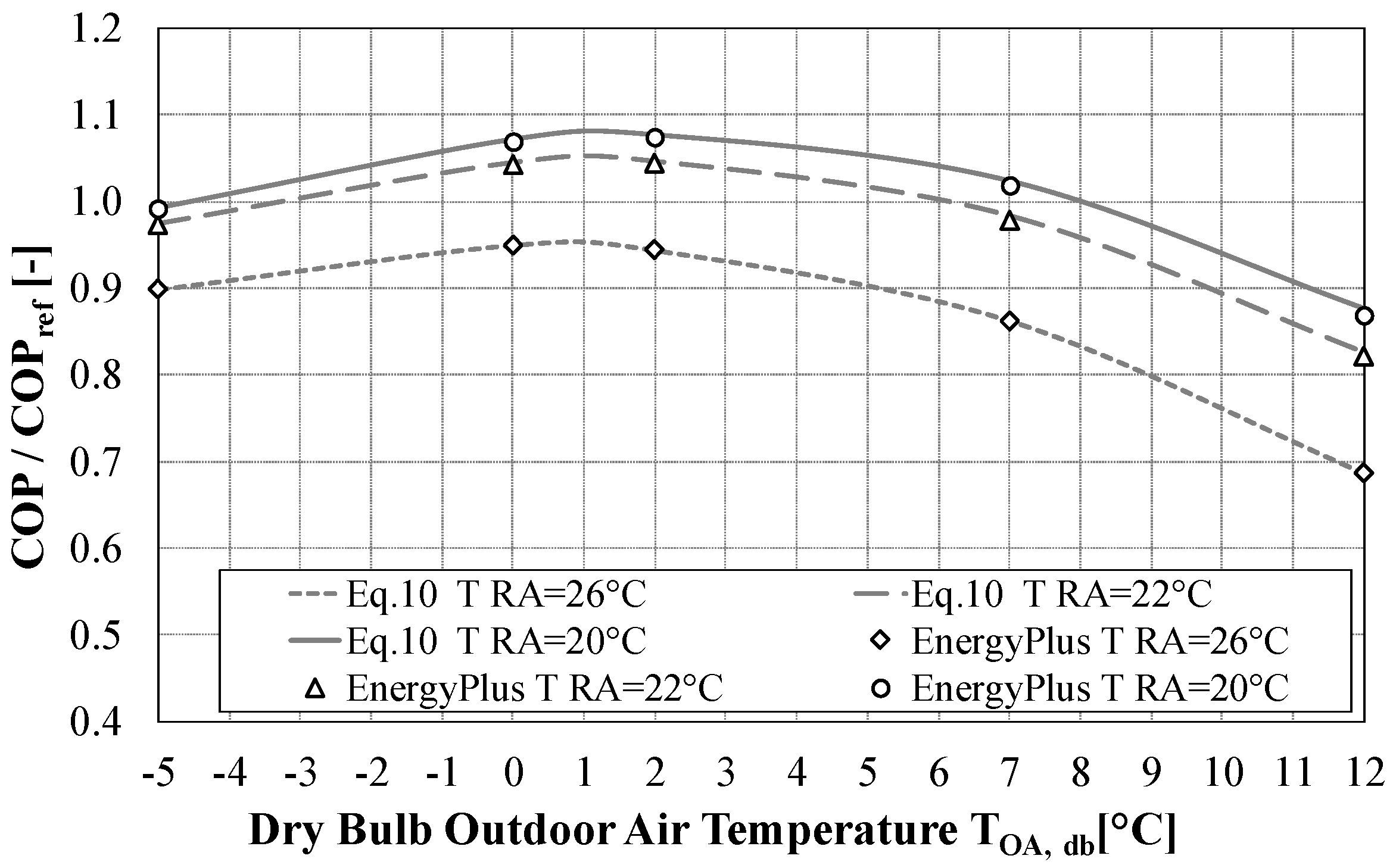
On the contrary, the performance parameter EIR (=1/EER) and COP depend on both the external and the return air temperature (Figure 4b and Figure 5b). In cooling mode, the EIR increases with the external air temperature TOA (load side temperature) and increases with the return air temperature TRA (source side temperature). In heating mode, the COP decreases as the return air temperature TRA is increased (source side temperature) whereas it decreases with the external air temperature (load side temperature) for TOA > 0 °C. For TOA < 0 °C, the COP increases with the external air temperature because of the energy consumption of the defrost contribution.
The agreement between manufacturer data and best-fit curves is good and the coefficients can be implemented in EnergyPlus to represent the behaviour of the present air-to-air heat pump. The average relative error (fit profiles vs. manufactured data) in cooling is about 2.3% for the cooling capacity and 3.3% for the EER. In heating mode, the average relative error is 2.4% for the heating capacity and 2.6% for the COP.
5. Results
5.1. Water-to-Water Heat Pump
The proposed “Curve Fit Method” presented in the previous paragraphs was validated with reference benchmark simulations in EnergyPlus.
A simplified model was created for this purpose, with a building able to work at nearly constant operating conditions for the whole simulation period, i.e., 1 month. The modelled building is equipped with the GCHP Clivet WSHN-XEE2 MF 14.2 and both cooling and heating modes are simulated. Different working conditions are analysed, imposing different load side outlet TL,out and source side inlet TS,in water temperature. The load of the building and the thermal response of the ground are properly calibrated to maintain the desired temperature difference at the source and load sides (Equations (11) and (12)).
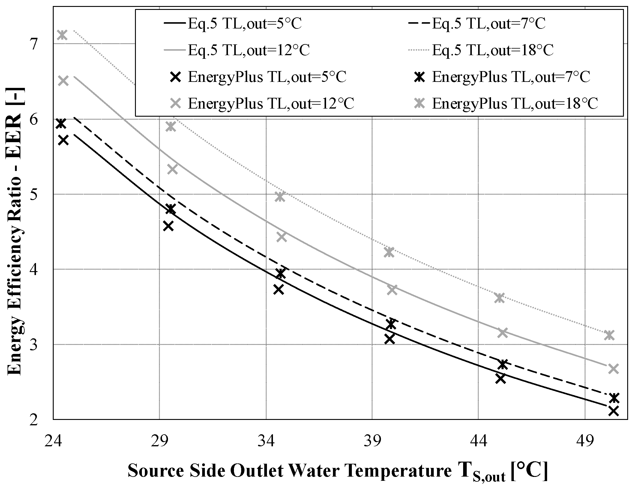
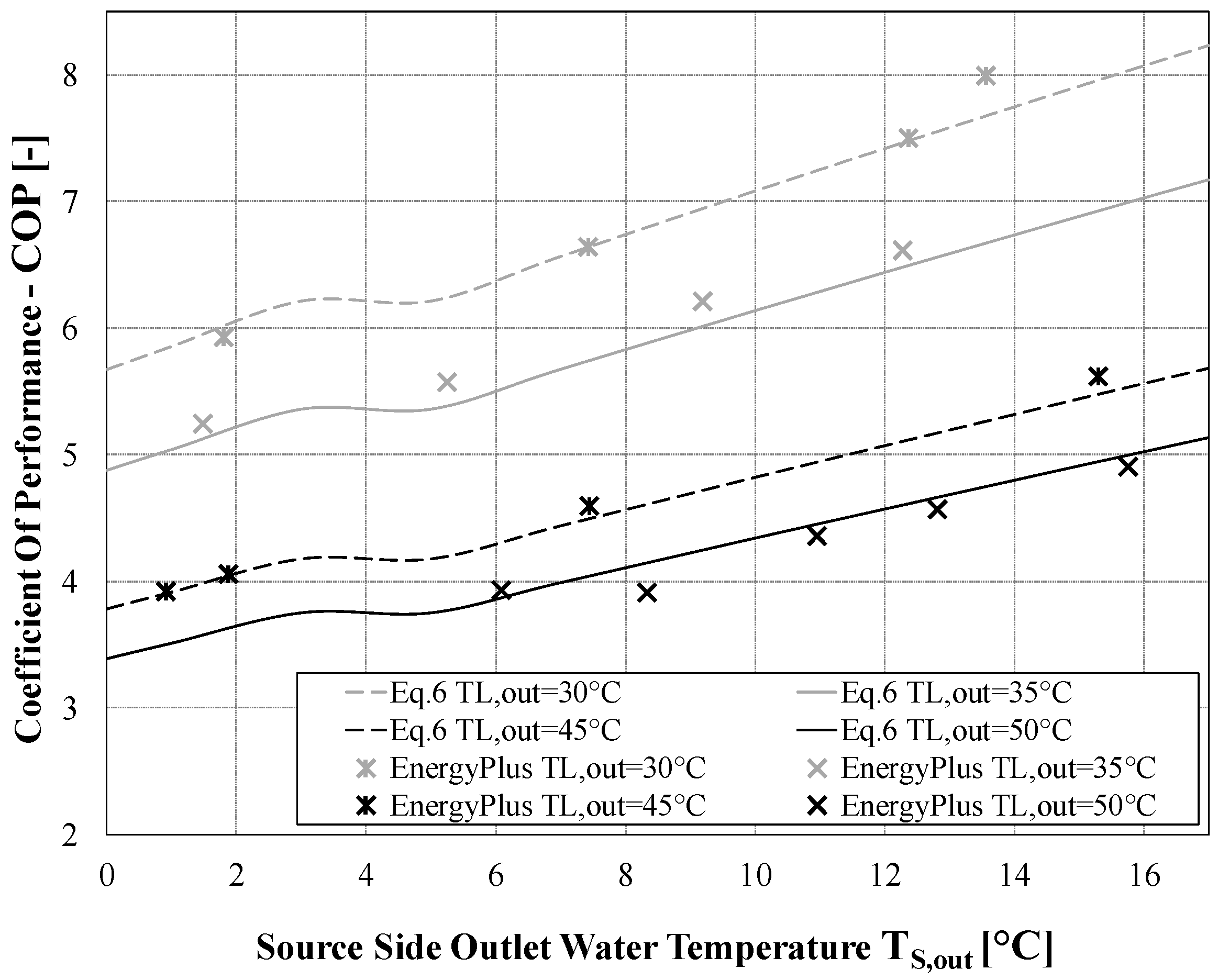
The results for the full load operating conditions are presented in Table A1 and Table A2 in Appendix A where the first two columns represent the imposed operating temperatures. From EnergyPlus simulations, it is possible to infer the inlet load and outlet source temperatures and verify that the temperature differences at the source and load sides are comparable to the desired values (Equations (11) and (12)). The performance values (EER and COP) are evaluated from the ratio between the simulated values of cooling or heating capacity and the electrical consumptions P. These simulated performances are then compared with the values calculated by means of the Curve Fit Method with a very good agreement.
5.2. Air-to-Air Heat Pump
The equation fit model approach was implemented in EnergyPlus also for the air-to-air heat pump, by means of Equations (7)–(10) with the coefficients in Table 7.
Similarly, in this case, a simplified building model was created with nearly constant operating conditions for the whole simulation duration, i.e., 1 month. The modelled building is equipped with the Clivet Zephir CPAN-XHE3 Size 3 and both cooling and heating are simulated.
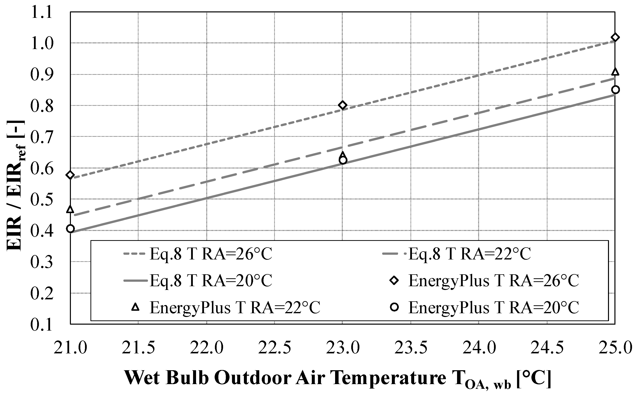
Different operating conditions were simulated, namely the ones presented in Table A3 and Table A4 in Appendix A for cooling and heating mode, respectively. In the tables, the results of EnergyPlus simulations are reported and compared with the data obtained with the implemented equation fit model. The agreement is very good, with an average relative error of almost 1.5% for the cooling capacity , 1.6% for the EER, 5.1% for the heating capacity and 0.26% for the COP. Figure 8 and Figure 9 show graphically the same comparison.
6. Conclusions
The aim of this work was to provide a series of insights to Energy Plus users when simulations are carried out taking into account the operating temperature effects on performance of heat pumps, chillers and even heat recovery heat pumps in ventilation circuits. The starting point was to refer to the equipment related to a recent near zero energy building at the Authors’ University. In particular, the final goal was to properly model the dependence of the heat pumps performance on the temperature, both load and source side and eventually on the partial load operating conditions. The actual installed water-to-water and air-to-air heat pumps have been considered and the equation fit model has been implemented with a series of modifications for adapting it to the typical data available from the manufacturer.
Coefficients needed in the equation fit models have been determined by means of an optimum search and, to validate the approach, a simplified building model equipped with the selected heat pumps and chiller has been created. The results from the simulations confirmed the expected results in terms of heating and cooling equipment performance at given nearly constant working temperatures even if small differences (within 7%) resulted from simulation trends and equation fit model input data. The relative error slightly increases (within 15%) if the partial load operating conditions are considered (PLF = 0.67, 0.33).
Author Contributions
The research and actions associated to writing the present paper are equally distributed among the three Authors. All authors have read and agreed to the published version of the manuscript.
Funding
This research received no external funding.
Conflicts of Interest
The authors declare no conflict of interest.
Appendix A

Table A1.
Benchmark simulations for the water-to-water heat pump (cooling case).
| Operating Conditions | Energy Plus Simulations | Simplified Curve Fit Method | |||||||
|---|---|---|---|---|---|---|---|---|---|
| TL,out [°C] | TS,in [°C] | TL,in [°C] | TS,out [°C] | Electric Power [W] | Cooling Capacity [W] | EER [-] | EERref [-] (Table 1) Interpolated | Tref [K] | EER [-] Equation (13) with coeff. Table 3 |
| 5 | 20 | 9.40 | 24.50 | 4500 | 25,699 | 5.71 | 5.55 | 283.15 | 5.72 |
| 5 | 25 | 9.18 | 29.43 | 5340 | 24,396 | 4.57 | 4.69 | 283.15 | 4.58 |
| 5 | 30 | 9.18 | 34.61 | 6544 | 24,396 | 3.73 | 3.98 | 283.15 | 3.73 |
| 5 | 35 | 9.18 | 39.82 | 7942 | 24,395 | 3.07 | 3.27 | 283.15 | 3.08 |
| 5 | 40 | 9.18 | 45.06 | 9582 | 24,394 | 2.55 | 2.67 | 283.15 | 2.55 |
| 5 | 45 | 9.18 | 50.35 | 11,535 | 24,392 | 2.11 | 2.13 | 283.15 | 2.12 |
| 7 | 20 | 11.31 | 24.38 | 4240 | 25,148 | 5.93 | 5.80 | 283.15 | 5.94 |
| 7 | 25 | 11.31 | 29.53 | 5244 | 25,148 | 4.80 | 4.68 | 283.15 | 4.80 |
| 7 | 30 | 11.31 | 34.70 | 6387 | 25,148 | 3.94 | 4.21 | 283.15 | 3.94 |
| 7 | 35 | 11.31 | 39.89 | 7701 | 25,148 | 3.27 | 3.51 | 283.15 | 3.27 |
| 7 | 40 | 11.31 | 45.12 | 9232 | 25,166 | 2.73 | 2.85 | 283.15 | 2.73 |
| 7 | 45 | 11.31 | 50.39 | 11,025 | 25,162 | 2.28 | 2.26 | 283.15 | 2.29 |
| 12 | 20 | 16.48 | 24.49 | 4016 | 26,105 | 6.50 | 6.34 | 283.15 | 6.51 |
| 12 | 25 | 16.48 | 29.62 | 4904 | 26,105 | 5.32 | 5.42 | 283.15 | 5.33 |
| 12 | 30 | 16.48 | 34.77 | 5898 | 26,105 | 4.43 | 4.65 | 283.15 | 4.43 |
| 12 | 35 | 16.48 | 39.93 | 7019 | 26,105 | 3.72 | 3.92 | 283.15 | 3.72 |
| 12 | 40 | 16.48 | 45.12 | 8293 | 26,105 | 3.15 | 3.18 | 283.15 | 3.15 |
| 12 | 45 | 16.48 | 50.34 | 9754 | 26,105 | 2.68 | 2.53 | 283.15 | 2.68 |
| 15 | 20 | 19.50 | 24.47 | 3845 | 26,193 | 6.81 | 6.75 | 283.15 | 6.82 |
| 15 | 25 | 19.50 | 29.60 | 4664 | 26,193 | 5.62 | 5.79 | 283.15 | 5.62 |
| 15 | 30 | 19.50 | 34.73 | 5574 | 26,193 | 4.70 | 4.98 | 283.15 | 4.71 |
| 15 | 35 | 20.07 | 40.02 | 6713 | 26,994 | 4.02 | 4.17 | 283.15 | 4.03 |
| 15 | 40 | 20.07 | 44.95 | 7505 | 25,743 | 3.43 | 3.45 | 283.15 | 3.43 |
| 15 | 45 | 20.07 | 50.01 | 8529 | 25,085 | 2.94 | 2.78 | 283.15 | 2.95 |
| 18 | 20 | 22.49 | 24.44 | 3674 | 26,118 | 7.11 | 7.04 | 283.15 | 7.12 |
| 18 | 25 | 22.49 | 29.55 | 4430 | 26,118 | 5.90 | 6.07 | 283.15 | 5.90 |
| 18 | 30 | 22.49 | 34.68 | 5265 | 26,118 | 4.96 | 5.27 | 283.15 | 4.97 |
| 18 | 35 | 22.49 | 39.81 | 6191 | 26,118 | 4.22 | 4.44 | 283.15 | 4.22 |
| 18 | 40 | 22.50 | 44.98 | 7244 | 26,196 | 3.62 | 3.63 | 283.15 | 3.62 |
| 18 | 45 | 22.50 | 50.16 | 8407 | 26,196 | 3.12 | 2.95 | 283.15 | 3.12 |
Table A2.
Benchmark simulations for the water-to-water heat pump (heating case).
| Operating Conditions | Energy Plus Simulations | Simplified Curve Fit Method | |||||||
|---|---|---|---|---|---|---|---|---|---|
| TL,out [°C] | TS,in [°C] | TL,in [°C] | TS,out [°C] | Electric Power [W] | Heating Capacity [W] | COP [-] | COPref [-] (Table 2) Interpolated | Tref [K] | COP Equation (16) with coeff. Table 3 |
| 30.0 | 6 | 24.6 | 1.8 | 10,000 | 59,092 | 5.91 | 5.95 | 283.15 | 5.92 |
| 30.0 | 10 | 24.6 | 7.4 | 9045 | 59,092 | 6.53 | 6.62 | 283.15 | 6.64 |
| 30.0 | 15 | 24.6 | 12.4 | 8006 | 59,092 | 7.38 | 7.42 | 283.15 | 7.49 |
| 30.0 | 18 | 24.6 | 13.6 | 7452 | 59,092 | 7.93 | 7.63 | 283.15 | 7.99 |
| 30.0 | 20 | 24.6 | 17.3 | 7108 | 59,092 | 8.31 | 8.28 | 283.15 | 8.31 |
| 34.6 | 6 | 28.7 | 1.5 | 12,260 | 65,200 | 5.32 | 5.13 | 283.15 | 5.24 |
| 34.6 | 8 | 28.7 | 5.2 | 11,642 | 65,200 | 5.60 | 5.48 | 283.15 | 5.57 |
| 34.6 | 12 | 28.7 | 9.2 | 10,525 | 65,200 | 6.19 | 6.04 | 283.15 | 6.20 |
| 35.0 | 15 | 29.0 | 12.3 | 9453 | 62,534 | 6.62 | 6.48 | 283.15 | 6.61 |
| 35.0 | 20 | 29.0 | 17.2 | 8383 | 62,534 | 7.46 | 7.21 | 283.15 | 7.36 |
| 45.0 | 5 | 38.5 | 0.9 | 16,101 | 63,962 | 3.97 | 3.88 | 283.15 | 3.92 |
| 45.0 | 6 | 38.5 | 1.9 | 15,649 | 63,962 | 4.09 | 3.98 | 283.15 | 4.06 |
| 45.0 | 10 | 38.5 | 7.4 | 14,015 | 63,962 | 4.56 | 4.52 | 283.15 | 4.59 |
| 45.0 | 18 | 38.5 | 15.3 | 11,398 | 63,962 | 5.61 | 5.42 | 283.15 | 5.61 |
| 45.0 | 20 | 38.5 | 17.3 | 10,848 | 63,962 | 5.90 | 5.68 | 283.15 | 5.86 |
| 50.0 | 8 | 42.8 | 6.1 | 13,108 | 50,297 | 3.84 | 3.70 | 283.15 | 3.93 |
| 49.6 | 13 | 46.1 | 8.3 | 11,169 | 43,586 | 3.90 | 3.91 | 283.15 | 3.90 |
| 50.0 | 10 | 44.9 | 10.9 | 11,911 | 51,803 | 4.35 | 4.16 | 283.15 | 4.35 |
| 50.0 | 15 | 45.1 | 12.8 | 11,982 | 54,673 | 4.56 | 4.34 | 283.15 | 4.56 |
| 50.0 | 18 | 45.1 | 15.8 | 11,151.4 | 54,673.3 | 4.90 | 4.66 | 283.15 | 4.90 |
| 50.0 | 20 | 45.1 | 17.7 | 10,665.7 | 54,673.3 | 5.13 | 4.88 | 283.15 | 5.13 |
Table A3.
Benchmark simulations for the air-to-air heat pump (cooling case).
| Cooling Mode | ||||||||||
|---|---|---|---|---|---|---|---|---|---|---|
| Operating Conditions | Energy Plus Simulations | Simplified Curve Fit Method | ||||||||
| TOAdb [°C] | TOAwb [°C] | TRAdb [°C] | TOAwb [°C] | TRAdb [°C] | Cooling Capacity [W] | Power [W] | EERS [-] | Cooling Capacity [W] | Power [W] | EERS [-] |
| 28 | 21 | 20 | 21.04 | 20.1 | 22,862.6 | 3538.5 | 6.5 | 23,241.9 | 3522.0 | 6.6 |
| 28 | 21 | 22 | 21.04 | 22.2 | 22,862.6 | 4062.9 | 5.6 | 23,241.9 | 3996.2 | 5.8 |
| 28 | 21 | 26 | 21.04 | 25.9 | 22,862.6 | 5024.3 | 4.6 | 23,241.9 | 5064.6 | 4.6 |
| 32 | 23 | 20 | 19.84 | 19.8 | 33,887.8 | 8078.1 | 4.2 | 33,792.4 | 7980.2 | 4.2 |
| 32 | 23 | 22 | 20.39 | 20.4 | 33,887.8 | 8264.8 | 4.1 | 33,792.4 | 8669.6 | 3.9 |
| 32 | 23 | 26 | 26.14 | 26.1 | 33,887.8 | 10,314.1 | 3.3 | 33,792.4 | 10,223.0 | 3.3 |
| 40 | 25 | 20 | 25.07 | 20.1 | 41,594.1 | 13,449.5 | 3.1 | 41,594.1 | 13,342.1 | 3.1 |
| 40 | 25 | 22 | 25.07 | 22.2 | 40,063.4 | 13,835.6 | 2.9 | 41,594.1 | 14,190.6 | 2.9 |
| 40 | 25 | 26 | 25.07 | 25.9 | 40,063.4 | 15,510.1 | 2.6 | 41,594.1 | 16,102.7 | 2.6 |
Table A4.
Benchmark simulations for the air-to-air heat pump (heating case).
| Heating Mode | |||||||||
|---|---|---|---|---|---|---|---|---|---|
| Operating Conditions | Energy Plus Simulations | Simplified Curve Fit Method | |||||||
| TOAdb [°C] | TRAdb [°C] | TOAdb [°C] | TRAdb [°C] | Heating Capacity [W] | Power [W] | COPS [-] | Heating Capacity [W] | Power [W] | COPS [-] |
| −5 | 20 | −5.0 | 20.01 | 45,426 | 10,007 | 4.54 | 49,292 | 10,873 | 4.5 |
| −5 | 22 | −5.0 | 21.99 | 45,426 | 9816 | 4.63 | 50,538 | 10,949 | 4.6 |
| −5 | 26 | −5.0 | 26.04 | 45,426 | 9071 | 5.01 | 50,814 | 10,147 | 5.0 |
| 0 | 20 | 0.0 | 20.03 | 46,609 | 11,077 | 4.21 | 47,425 | 11,298 | 4.2 |
| 0 | 22 | 0.0 | 21.99 | 46,603 | 10,787 | 4.32 | 48,407 | 11,241 | 4.3 |
| 0 | 26 | 0.0 | 25.98 | 46,606 | 9838 | 4.74 | 48,152 | 10,164 | 4.7 |
| 2 | 20 | 2.0 | 20.01 | 43,530 | 10,393 | 4.19 | 45,651 | 10,928 | 4.2 |
| 2 | 22 | 2.0 | 21.94 | 43,547 | 10,100 | 4.31 | 46,526 | 10,819 | 4.3 |
| 2 | 26 | 2.0 | 26.03 | 43,439 | 9111 | 4.77 | 46,059 | 9661 | 4.8 |
| 7 | 20 | 7.0 | 20.10 | 35,889 | 8124 | 4.42 | 38,645 | 8793 | 4.4 |
| 7 | 22 | 7.0 | 22.01 | 35,885 | 7804 | 4.60 | 39,254 | 8582 | 4.6 |
| 7 | 26 | 7.0 | 26.30 | 35,885 | 6878 | 5.22 | 38,258 | 7332 | 5.2 |
| 12 | 20 | 12.0 | 20.08 | 28,062 | 5421 | 5.18 | 27,966 | 5443 | 5.1 |
| 12 | 22 | 12.0 | 21.99 | 28,206 | 5144 | 5.48 | 28,311 | 5199 | 5.4 |
| 12 | 26 | 12.0 | 25.93 | 26,784 | 4085 | 6.56 | 26,784 | 4085 | 6.6 |
References
- Official Website of the European Union—Energy Performance of Buildings. Available online: https://ec.europa.eu/energy/en/topics/energy-efficiency/energy-performance-of-buildings (accessed on 10 February 2020).
- Silenzi, F.; Priarone, A.; Fossa, M. Hourly simulations of a hospital building for assessing the thermal demand and the best retrofit strategies for consumption reduction. Therm. Sci. Eng. Prog. 2018, 6, 388–397. [Google Scholar] [CrossRef] [Green Version]
- Linzi, Z.; Joseph, L. Environmental and economic evaluations of building energy retrofits: Case study of a commercial building. Build. Environ. 2018, 145, 14–23. [Google Scholar]
- Liang, J.; Qiu, Y.; James, T.; Ruddell, B.L.; Dalrymple, M.; Earl, S.; Castelazo, A. Do energy retrofits work? Evidence from commercial and residential buildings in Phoenix. J. Environ. Econ. Manag. 2018, 92, 726–743. [Google Scholar] [CrossRef]
- Casquero-Modrego, N.; Goñi-Modrego, M. Energy retrofit of an existing affordable building envelope in Spain, case study. Sustain. Cities Soc. 2019, 44, 395–405. [Google Scholar] [CrossRef]
- Kumar, G.K.; Saboor, S.; Kumar, V.; Kim, K.; Babu, A.T.P. Experimental and theoretical studies of various solar control window glasses for the reduction of cooling and heating loads in buildings across different climatic regions. Energy Build. 2018, 173, 326–336. [Google Scholar]
- Chahine, K.; Murr, R.; Ramadan, M.; El Hage, H.; Khaled, M. Use of parabolic troughs in HVAC applications–Design calculations and analysis. Case Stud. Therm. Eng. 2018, 12, 285–291. [Google Scholar] [CrossRef]
- Soltani, M.; Kashkooli, F.M.; Dehghani-Sanij, A.R.; Kazemi, A.R.; Bordbar, N.; Farshchi, M.J.; Elmi, M.; Gharali, K.; Dusseault, M.B. A comprehensive study of geothermal heating and cooling systems. Sustain. Cities Soc. 2019, 44, 793–818. [Google Scholar] [CrossRef]
- Sebarchievici, C.; Sarbu, I. Performance of an experimental ground-coupled heat pump system for heating, cooling and domestic hot-water operation. Renew. Energy 2015, 76, 148–159. [Google Scholar] [CrossRef]
- Lee, J.; Kim, T.; Leigh, S. Thermal performance analysis of a ground-coupled heat pump integrated with building foundation in summer. Energy Build. 2013, 59, 37–43. [Google Scholar] [CrossRef]
- Qi, D.; Pu, L.; Ma, Z.; Xia, L.; Li, Y. Effects of ground heat exchangers with different connection configurations on the heating performance of GSHP systems. Geothermics 2019, 80, 20–30. [Google Scholar] [CrossRef]
- Lee, S.H.; Jeon, Y.; Chung, H.J.; Cho, W.; Kim, Y. Simulation-based optimization of heating and cooling seasonal performances of an air-to-air heat pump considering operating and design parameters using genetic algorithm. Appl. Therm. Eng. 2018, 144, 362–370. [Google Scholar] [CrossRef]
- Torregrosa-Jaime, B.; Martínez, P.J.; González, B.; Payá-Ballester, G. Modelling of a variable refrigerant flow system in EnergyPlus for building energy simulation in an Open Building Information modelling environment. Energies 2019, 12, 22. [Google Scholar] [CrossRef] [Green Version]
- Fisher, D.E.; Rees, S.J.; Padhmanabhan, S.K.; Murugappan, A. Implementation and validation of ground-source heat pump system models in an integrated building and system simulation environment. HVAC R Res. 2006, 12 (Suppl. 1), 693–710. [Google Scholar] [CrossRef]
- Jin, H. Parameter Estimation Based Models of Water Source Heat Pumps. Ph.D. Thesis, Oklahoma State University, Stillwater, OK, USA, 2002. [Google Scholar]
- Tang, C. Modeling Packaged Heat Pumps in a Quasi-Steady State Energy Simulation Program. Master’s Thesis, Oklahoma State University, Stillwater, OK, USA, 2005. [Google Scholar]
- Murugappan, A. Implementing Ground Source Heat Pump and Ground Loop Heat Exchanger Models in the Energyplus Simulation Environment. Master’s Thesis, Oklahoma State University, Stillwater, OK, USA, 2002. [Google Scholar]
- EnergyPlus Development Team. EnergyPlus Version 9.1 Engineering Reference: The Reference to EnergyPlus Calculations; EnergyPlus Development Team, US Department of Energy: Washington, DC, USA, 2019.
- Fossa, M.; Minchio, F. The effect of borefield geometry and ground thermal load profile on hourly thermal response of geothermal heat pump systems. Energy 2013, 51, 323–329. [Google Scholar] [CrossRef]
- Zephir CPAN-XHE3: Technical Bullettin; Clivet: Belluno, Italy, 2016.
Figure 1.
Scheme of HP operating conditions, (a) water-to-water HP, (b) air-to-air HP (without heat recovery).
Figure 1.
Scheme of HP operating conditions, (a) water-to-water HP, (b) air-to-air HP (without heat recovery).

Figure 2.
(a) QC/QC ref and (b) P/P ref comparison for cooling mode.


Figure 3.
(a) QH/QH ref and (b) P/P ref comparison for heating mode.


Figure 4.
Cooling capacity (a) and HP performance (b) in cooling mode: comparison between Table 5 and Equations (7) and (8) with Table 7 coefficients.


Figure 5.
Heating capacity (a) and HP performance (b) in heating mode: comparison between Table 6 and Equations (9) and (10) with Table 7 coefficients.

Figure 6.
EER in cooling mode: comparison between EnergyPlus simulations and equation fit model approach.
Figure 6.
EER in cooling mode: comparison between EnergyPlus simulations and equation fit model approach.

Figure 7.
COP in heating mode: comparison between EnergyPlus simulations and equation fit model approach.
Figure 7.
COP in heating mode: comparison between EnergyPlus simulations and equation fit model approach.

Figure 8.
EIR in cooling mode: comparison between EnergyPlus simulations and Equation (8) with Table 6 coefficients.
Figure 8.
EIR in cooling mode: comparison between EnergyPlus simulations and Equation (8) with Table 6 coefficients.

Figure 9.
COP in heating mode: comparison between EnergyPlus simulations and Equation (10) with Table 6 coefficients.
Figure 9.
COP in heating mode: comparison between EnergyPlus simulations and Equation (10) with Table 6 coefficients.

Table 1.
Manufacturer data for reversible heat pump. The data are from Clivet manufacturer for HP model WSHN-XEE2 MF 14.2. Cooling Mode.
Table 1.
Manufacturer data for reversible heat pump. The data are from Clivet manufacturer for HP model WSHN-XEE2 MF 14.2. Cooling Mode.
| Source Side Outlet Water Temperature, TS,out [°C] | Load Side Outlet Water Temperature, TL,out [°C] | |||||||||||||||||
|---|---|---|---|---|---|---|---|---|---|---|---|---|---|---|---|---|---|---|
| 5 | 7 | 10 | 12 | 15 | 18 | |||||||||||||
| kWt | kWe | EER | kWt | kWe | EER | kWt | kWe | EER | kWt | kWe | EER | kWt | kWe | EER | kWt | kWe | EER | |
| 25 | 41.7 | 7.67 | 5.43 | 44.3 | 7.75 | 5.72 | 48.1 | 7.89 | 6.10 | 50 | 8 | 6.25 | 54.6 | 8.2 | 6.66 | 58.9 | 8.51 | 6.92 |
| 30 | 39.9 | 8.67 | 4.60 | 42.5 | 8.76 | 4.86 | 46.1 | 8.89 | 5.19 | 48.1 | 9 | 5.34 | 52.4 | 9.18 | 5.71 | 56.6 | 9.46 | 5.98 |
| 35 | 38.1 | 9.67 | 3.93 | 40.7 | 9.76 | 4.17 | 44.1 | 9.89 | 4.46 | 46.2 | 10 | 4.62 | 50.1 | 10.16 | 4.93 | 54.3 | 10.4 | 5.22 |
| 40 | 35.4 | 10.92 | 3.24 | 38.3 | 10.9 | 3.50 | 41.6 | 11.1 | 3.75 | 43.5 | 11.1 | 3.92 | 47.3 | 11.3 | 4.19 | 51.3 | 11.6 | 4.42 |
| 45 | 32.9 | 12.3 | 2.68 | 35.3 | 12.4 | 2.86 | 38.2 | 12.5 | 3.06 | 40.2 | 12.6 | 3.19 | 43.6 | 12.7 | 3.43 | 47.2 | 13 | 3.63 |
| 50 | 29.8 | 13.8 | 2.16 | 32 | 13.9 | 2.30 | 34.8 | 14 | 2.49 | 36.5 | 14.1 | 2.59 | 39.9 | 14.3 | 2.79 | 43.1 | 14.5 | 2.97 |
Table 2.
Manufacturer Data for reversible heat pump. The data are from Clivet manufacturer for HP model WSHN-XEE2. Heating Mode.
Table 2.
Manufacturer Data for reversible heat pump. The data are from Clivet manufacturer for HP model WSHN-XEE2. Heating Mode.
| Source Side Outlet Water Temperature, TS,out [°C] | Load Side Outlet Water Temperature, TL,out [°C] | |||||||||||
|---|---|---|---|---|---|---|---|---|---|---|---|---|
| 30 | 35 | 45 | 50 | |||||||||
| kWt | kWe | COP | kWt | kWe | COP | kWt | kWe | COP | kWt | kWe | COP | |
| 0 | 41.8 | 7.37 | 5.67 | 41.3 | 8.35 | 4.95 | 40.5 | 10.7 | 3.79 | 39.4 | 12.2 | 3.23 |
| 1 | 43.1 | 7.39 | 5.83 | 42.4 | 8.37 | 5.07 | 41.6 | 10.7 | 3.89 | 40.4 | 12.2 | 3.32 |
| 3 | 45.5 | 7.44 | 6.12 | 44.9 | 8.43 | 5.33 | 43.8 | 10.7 | 4.10 | 42.6 | 12.2 | 3.50 |
| 5 | 46.5 | 7.47 | 6.22 | 46.3 | 8.48 | 5.45 | 45.4 | 10.7 | 4.24 | 43.8 | 12.2 | 3.59 |
| 7 | 49.4 | 7.53 | 6.55 | 49.0 | 8.54 | 5.73 | 48.0 | 10.7 | 4.48 | 46.25 | 12.2 | 3.79 |
| 10 | 53.7 | 7.62 | 7.04 | 53.2 | 8.65 | 6.15 | 51.8 | 10.8 | 4.79 | 49.85 | 12.25 | 4.07 |
| 12 | 56.7 | 7.70 | 7.36 | 56.2 | 8.73 | 6.44 | 54.7 | 10.9 | 5.02 | 52.55 | 12.35 | 4.26 |
| 15 | 61.7 | 7.83 | 7.88 | 60.9 | 8.86 | 6.87 | 59.2 | 11.0 | 5.38 | 56.75 | 12.4 | 4.58 |
| 17 | 65.2 | 7.92 | 8.24 | 64.4 | 8.96 | 7.19 | 62.5 | 11.0 | 5.68 | 59.85 | 12.45 | 4.81 |
Table 3.
Manufacturer data for Clivet model WSHN-XEE2. Effect of PLF on the HP performance.
| PLF | EER/EERfull load | COP/COPfull load |
|---|---|---|
| 0.33 | 1.080 | 1.146 |
| 0.67 | 1.032 | 1.103 |
| 1 | 1.000 | 1.000 |
Table 4.
Calculated coefficients for the “Curve Fit Method” for the water-to-water HP.
| A1 | 0.957 | D1 | 0.088 |
| A2 | 0.407 | D2 | −0.090 |
| A3 | −1.326 | D3 | 0.012 |
| A4 | 0.076 | D4 | 0.992 |
| A5 | 0.916 | D5 | 0.001 |
| B1 | −5.181 | E1 | 1.100 |
| B2 | −1.927 | E2 | 8.056 |
| B3 | 6.627 | E3 | −10.091 |
| B4 | −1.503 | E4 | 1.862 |
| B5 | 2.930 | E5 | 0.089 |
Table 5.
Datasheet values in cooling mode for present study analyses (manufacturer data in gray). Air handling unit model Zephir CPAN-XHE3 (air flow 4600 m3/h, supply humidity ratio 11 gvap/kgair).
Table 5.
Datasheet values in cooling mode for present study analyses (manufacturer data in gray). Air handling unit model Zephir CPAN-XHE3 (air flow 4600 m3/h, supply humidity ratio 11 gvap/kgair).
| Reference Conditions | |||||
| Ref. External Air Temperature (Dry-Bulb) TOAdb [°C] | Ref. External Air Temperature (Wet-Bulb) TOAwb [°C] | Ref. Return Air Temperature (Dry-Bulb) TRAdb [°C] | Ref. Cooling Capacity [W] | Ref. Compressor + Fan Power [W] | Ref. EER [-] |
| 40 | 25 | 26 | 41,900 | 16,115 | 2.6 |
| Performance Data | |||||
| External AIR Temperature (Dry-Bulb) TOAdb [°C] | External Air Temperature (Wet-Bulb) TOAwb [°C] | Return Air Temperature (Dry-Bulb) TRAdb [°C] | Cooling Capacity [W] | Compressor + Fan Power [W] | EER [-] |
| 40 | 25 | 26 | 41,900 | 16,115 | 2.60 |
| 35 | 24 | 26 | 38,700 | 13,345 | 2.90 |
| 32 | 23 | 26 | 34,000 | 10,000 | 3.40 |
| 30 | 22 | 26 | 29,100 | 6929 | 4.20 |
| 28 | 21 | 26 | 23,600 | 4917 | 4.80 |
| 25 | 19 | 26 | 8100 | 2132 | 3.80 |
| 40 | 25 | 22 | 41,900 | 14,249 | 2.94 |
| 35 | 24 | 22 | 38,700 | 12,009 | 3.22 |
| 32 | 23 | 22 | 34,000 | 8794 | 3.87 |
| 30 | 22 | 22 | 29,100 | 6095 | 4.77 |
| 28 | 21 | 22 | 23,600 | 4292 | 5.50 |
| 25 | 19 | 22 | 8100 | 1735 | 4.67 |
| 40 | 25 | 20 | 41,900 | 13,383 | 3.13 |
| 35 | 24 | 20 | 38,700 | 11,273 | 3.43 |
| 32 | 23 | 20 | 34,000 | 8224 | 4.13 |
| 30 | 22 | 20 | 29,100 | 5675 | 5.13 |
| 28 | 21 | 20 | 23,600 | 3971 | 5.94 |
| 25 | 19 | 20 | 8100 | 1515 | 5.35 |
Table 6.
Datasheet values in heating mode for present study analyses (manufacturer data in gray). Air handling unit model Zephir CPAN-XHE3 (air flow 4600 m3/h).
Table 6.
Datasheet values in heating mode for present study analyses (manufacturer data in gray). Air handling unit model Zephir CPAN-XHE3 (air flow 4600 m3/h).
| Reference Conditions | ||||
| Ref. External Air Temperature (Dry-Bulb) TOAdb [°C] | Ref. Return Air Temperature (Dry-Bulb) TRAdb [°C] | Ref. Heating Capacity [W] | Ref. Compressor + Fan Power [W] | Ref. COP [-] |
| −5 | 20 | 49,700 | 11,044 | 4.50 |
| Performance Data | ||||
| External Air Temperature (Dry-Bulb) TOAdb [°C] | Return Air Temperature (Dry-Bulb) TRAdb [°C] | Heating Capacity [W] | Compressor + fan power [W] | COP [-] |
| −5 | 20 | 49,700 | 11,044 | 4.50 |
| 0 | 20 | 49,500 | 12,375 | 4.00 |
| 2 | 20 | 46,200 | 11,268 | 4.10 |
| 7 | 20 | 37,100 | 8065 | 4.60 |
| 12 | 20 | 28,400 | 5462 | 5.20 |
| −5 | 22 | 49,700 | 10,592 | 4.69 |
| 0 | 22 | 49,500 | 11,717 | 4.22 |
| 2 | 22 | 46,200 | 10,738 | 4.30 |
| 7 | 22 | 37,100 | 7712 | 4.81 |
| 12 | 22 | 28,400 | 5254 | 5.41 |
| −5 | 26 | 49,700 | 9469 | 5.25 |
| 0 | 26 | 49,500 | 10,633 | 4.66 |
| 2 | 26 | 46,200 | 9703 | 4.76 |
| 7 | 26 | 37,100 | 6868 | 5.40 |
| 12 | 26 | 28,400 | 4605 | 6.17 |
Table 7.
Calculated coefficients for the “Equation Fit Approach”, air-to-air heat pump.
| a0 | −6.04980 | b0 | −2.20000 | c0 | −0.06076 | d0 | 0.59269 |
| a1 | 0.48670 | b1 | 0.11000 | c1 | −0.00423 | d1 | 0.02513 |
| a2 | −0.00820 | b2 | 0.00000 | c2 | −0.00148 | d2 | −0.00190 |
| a3 | 0.00000 | b3 | 0.00300 | c3 | 0.08791 | d3 | 0.05807 |
| a4 | 0.00000 | b4 | 0.00056 | c4 | −0.00186 | d4 | −0.00171 |
| a5 | 0.00000 | b5 | 0.00000 | c5 | −0.00053 | d5 | −0.00094 |
© 2020 by the authors. Licensee MDPI, Basel, Switzerland. This article is an open access article distributed under the terms and conditions of the Creative Commons Attribution (CC BY) license (http://creativecommons.org/licenses/by/4.0/).
Share and Cite
MDPI and ACS Style
Priarone, A.; Silenzi, F.; Fossa, M. Modelling Heat Pumps with Variable EER and COP in EnergyPlus: A Case Study Applied to Ground Source and Heat Recovery Heat Pump Systems. Energies 2020, 13, 794. https://doi.org/10.3390/en13040794
AMA Style
Priarone A, Silenzi F, Fossa M. Modelling Heat Pumps with Variable EER and COP in EnergyPlus: A Case Study Applied to Ground Source and Heat Recovery Heat Pump Systems. Energies. 2020; 13(4):794. https://doi.org/10.3390/en13040794
Chicago/Turabian StylePriarone, Antonella, Federico Silenzi, and Marco Fossa. 2020. "Modelling Heat Pumps with Variable EER and COP in EnergyPlus: A Case Study Applied to Ground Source and Heat Recovery Heat Pump Systems" Energies 13, no. 4: 794. https://doi.org/10.3390/en13040794
Note that from the first issue of 2016, this journal uses article numbers instead of page numbers. See further details here.