Article

Assessing Financial and Flexibility Incentives for Integrating Wind Energy in the Grid Via Agent-Based Modeling

1
Electrical Energy Laboratory (EELAB), Department of Electromechanical, Systems and Metal Engineering, Ghent University, Tech Lane Ghent Science Park—Campus A, Technologiepark-Zwijnaarde 131, 9052 Ghent, Belgium
2
Sharif Policy Research Institute (SPRI), Sharif University of Technology, Tehran 1459986131, Iran
*
Author to whom correspondence should be addressed.
Energies 2019, 12(22), 4314; https://doi.org/10.3390/en12224314
Submission received: 12 September 2019 / Revised: 21 October 2019 / Accepted: 7 November 2019 / Published: 12 November 2019
(This article belongs to the Special Issue 100% Renewable Energy Transition: Pathways and Implementation)

Abstract

:
This article provides an agent-based model of a hypothetical standalone electricity network to identify how the feed-in tariffs and the installed capacity of wind power, calculated in percentage of total system demand, affect the electricity consumption from renewables. It includes the mechanism of electricity pricing on the Day Ahead Market (DAM) and the Imbalance Market (IM). The extra production volumes of Electricity from Renewable Energy Sources (RES-E) and the flexibility of electrical consumption of industries is provided as reserves on the IM. Five thousand simulations were run by using the agent-based model to gather data that were then fit in linear regression models. This helped to quantify the effect of feed-in tariffs and installed capacity of wind power on the consumption from renewable energy and market prices. The consumption from renewable sources, expressed as percentage of total system consumption, increased by 8.17% for every 10% increase in installed capacity of wind power. The sharpest increase in renewable energy consumption is observed when a feed-in tariff of 0.04 €/kWh is provided to the wind farm owners, resulting in an average increase of 9.1% and 5.1% in the consumption from renewable sources while the maximum installed capacity of wind power is 35% and 100%, respectively. The regression model for the annualized DAM prices showed an increase by 0.01 €cents/kWh in the DAM prices for every 10% increase in the installed wind power capacity. With every increase of 0.01 €/kWh in the value of feed-in tariffs, the mean DAM price is lowered as compared to the previous value of the feed-in tariff. DAM prices only decrease with increasing installed wind capacity when a feed-in tariff of 0.04 €/kWh is provided. This is observed because all wind power being traded on DAM at a very cheap price. Hence, no volume of electricity is being stored for availability on IM. The regression models for predicting IM prices show that, with every 10% increase in installed capacity of wind power, the annualized IM price decreases by 0.031 and 0.34 €cents/kWh, when installed capacity of wind power is between 0 and 25%, and between 25 and 100%, respectively. The models also showed that, until the maximum installed capacity of wind power is less than 25%, the IM prices increase when the value of feed-in tariff is 0.01 and 0.04 €/kWh, but decrease for a feed-in tariff of 0.02 and 0.03 €/kWh. When installed capacity of wind power is between 25 and 100%, increasing feed-in tariffs to the value of 0.03 €/kWh result in lowering the mean IM price. However, at 0.04 €/kWh, the mean IM price is higher, showing the effect of no storage reserves being available on IM and more expensive reserves being engaged on the IM. The study concludes that the effect of increasing installed capacity of wind power is more significant on increasing consumption of renewable energy and decreasing the DAM and IM prices than the effect of feed-in tariffs. However, the effect of increasing values of both factors on the profit of RES-E producers with storage facilities is not positive, pointing to the need for customized rules and incentives to encourage their market participation and investment in storage facilities.

Graphical Abstract

1. Introduction

In 2017, with 17% contribution of renewables in the total energy needs, the EU was well on the way to achieve the 2020 target of 20% renewables [1]. As the EU Renewable Energy Directive aims to increase this number to 32% in 2030 [2], considerable investments and infrastructural changes are needed in the European member states to accommodate renewables in the energy mix. In 2018, 26.7 billion Euros were spent alone on wind energy projects, of which 16.4 billion was spent solely on onshore wind energy [3].
Different market integration schemes and support mechanisms have been developed for increasing the injection of Electricity from Renewable Energy Sources (RES-E) in the grid and to restrict the costs induced by the variability and limited predictability of RES-E generation. In liberalized power markets, these costs occur as imbalance costs, which may be defined as a penalty for deviating from the submitted production and consumption plan [4]. In extreme cases, the unpredictable RES-E that are protected from the market effects by different financial incentives, like the tradable green certificates and the feed-in tariffs contribute to causing a negative market price [4,5,6]. Investment grants, RES-E quotas, feed-in-tariffs, green certificates, etc. also generate incentives to invest, which indirectly increase competition and improve technology leading to cost reductions and volume growth [7]. Eventually, the RES-E push the expensive systems like nuclear and gas fired power plants out of the market and lower the market price due to their negligible marginal costs. However, this increases price volatility on the market. Extremely high prices are caused when demand peaks as compared to the supply.
Traditionally, established technologies of power production, e.g., coal-fired, gas-fired or nuclear power plants, were used to provide the needed ancillary services to the grid, maintaining a safe operation. However, since renewables have successfully entered the electricity market, the need for system security has increased. It is estimated that, for every 8 MW of wind power installed, a 1 MW of peaking plant is required [8], whereas, it is also estimated that most of the peaking gas units today operate at below 20% utilization rates [9]. Use of demand side response (DSR) as a grid balancing strategy is a recent phenomenon [10], but it shows promising potential, especially when coupled with increased wind power injection [11]. DSR is a set of measures that uses loads, local generation, and storage to support network operations and also to enhance the quality of power supply [12]. DSR has been proven to reduce the needed conventional generation capacity, to maximize the low carbon generation, to contribute to short-term system balancing and to defer the network reinforcements [13]. This article studies the effect of limited generational flexibility of the wind farms that receive a feed-in tariff for each kWh of renewable power they inject in the grid, against the reserves provided by the industries and other technologies as flexible demand.
Electricity grid and markets are composed of multiple actors, who are engaged in consumption/production of electricity that fulfill their own needs and businesses. Their interactions via the market and the electricity grid results in impacting the consumption/production pattern of each other. Agent-based modelling allows to mimic the behavior of human beings and simulate production, consumption and bidding processes, in which participants are modeled as adaptive agents with different strategies [14]. Agent-Based Models (ABMs) have been used to model the diffusion of energy efficient technologies through the society by the interaction of different agents [15,16]. ABMs are used to explore possible states of a system to understand plausible futures, trends, tendencies, and behaviors that can occur under specific circumstances [17].
Previous work on the use of ABMs for electricity grids, markets, and the injection of renewables have focused on the effect of prosumption and peer to peer supply and its effect on the grid management [18] and grid design strategies [19]. ABMs have also been used to predict price of energy trading in smart grids by the use of incomplete information by different agents to optimize their own utility [20]. Likewise, they have been employed as an e-laboratory to test different regulatory interventions before implementation [21]. Furthering the investigation on the profit RES-E producers, ABM has been used to study the optimum conditions for the wind power producers participating in a deregulated market with the inclusion of learning algorithms to optimize the bidding process [14]. Similarly, the technique has been employed to investigate the effect of storage possibilities in the form of electric vehicles on the profit of wind farms that engage in the electricity markets [22]. Based on the above-mentioned examples of application of ABMs for decision-making, technology diffusion, and market price calculation, the data for analysis were generated by an ABM that was developed specifically for this study.

1.1. Electricity Markets and Grid Balancing

Energy system flexibility is not a technological issue alone; it has a strong link to the energy markets as well [23]. Balancing the potential supply and demand of electricity at any given time ensures a reliable supply of electricity. Transmission System Operators (TSOs) are entrusted to carry out the necessary security checks and real-time operations of ensuring a smooth supply of electricity to the consumers [6]. To make this possible, the majority of electricity trade is conducted up to one day before delivery. Based on the time dimension, energy trade is divided into different markets in Europe. In this article, a Day Ahead Market (DAM) and an Imbalance Market (IM) are modeled based on the principles of the same markets in Belgium [24,25]. To ensure more transparent market pricing system, in both markets, buyers and sellers trade electricity following an energy exchange. For the DAM, the intersection of scheduled production and consumption profiles provide the market prices for each hour of the next day, as shown in Figure 1a. The RES-E technologies have the lowest marginal costs as compared to the other technologies and hence are the first ones in the order. The effect of RES pushes the supply curve to the right, and this is shown in Figure 1b.
The potential forecasts for demand can be faulty and may still cause imbalances in real time, coupled with increased unpredictability due to increased injection of wind power resulting in higher demand for reserves [20]. IM or the balancing market represents the market where the trade of deviations from the scheduled market positions is dealt with [21]. A real-time balancing market is particularly useful for RES-E as they can provide higher forecast reliability closer to real time [6]. Due to the very fast response times required to balance this market and the connected security issues, this market is coordinated by the TSO [22]. Conventionally, TSOs contract minimum reserve from firm capacity, or power plants with technology that can be easily ramped up and down to balance the grid. Recently, regardless of the source technology, reserves are being contracted by the TSOs. Together, these reserves form the activation price ladder that is shown in Figure 2. The terminology, cheap, mid-priced, and expensive, refers to how much the TSO will have to pay for the reserves in case of grid imbalance.
In order to ensure system security, TSOs procure balancing services from balancing service providers. Instead of balancing service providers, in this article, we deal with the market participants, called agents, who are the RES-E producers and industries as consumers and reserve providers. These agents are responsible for keeping their portfolio balanced for a given period of time. An agent’s portfolio is defined by its nature. For the producers, the portfolio refers to the injection and also off-take if it has storage facilities; for the industries, it is the consumption profile, which can alter in both directions to provide the necessary response to grid imbalance.
Following the IM pricing mechanism in Belgium, in this article, we also modeled a one-price settlement mechanism for the IM. This represents the settlement side of the reserve market, where a price is quoted every quarter of an hour, which represents the marginal activation cost of the reserves.

1.2. Hypothesis Formulation

Feed-in tariffs have proven to be superior for wind power promotion in countries like Denmark, Germany, and Spain [26,27], as cited by [28], but such a system does not force the RES-E producers to operate cost efficiently [28]. Although the subsidies for RES-E producers are slowly being phased out, the question is if the subsidies are negatively affecting the unharnessed potential of DSR as a means to accommodate RES-E in the existing electricity network.
This is especially relevant for countries, like Belgium, where old and outdated nuclear or fossil fuel power plants are scheduled to be decommissioned. In the period of 2020–2025, 5000 MW of nuclear energy is scheduled to be phased-out when seven nuclear reactors will be shut down in Belgium [29]. If the phase-out is carried through, it is speculated that Belgium’s carbon footprint will deteriorate, as the firm capacity will need to be replaced by fossil-based power plants. However, if Belgium replaces non-renewable power technologies with RES-E technologies, the effects on the grid balancing and market prices will be significant.
Currently, a feed-in tariff of 0.04 €/kWh is given to Belgian RES-E producers for every kWh of wind energy injected into the grid [30]—while the installed wind capacity accounts for 13.2% of the total installed power capacity [31]. Using Belgium’s example, we assessed varying levels of feed-in tariffs (τ) (0.01, 0.02, 0.03 and 0.04 €/kWh) for their effect on the consumption of renewable energy from the grid. Likewise, the effect of increasing the installed capacity of wind farms (∆x) is tested to observe which of the two factors; τ or ∆x, has a higher impact on increasing injection of wind energy in the grid. Although the example of Belgium is quoted here to design the experiments, our aim is to gain a principle mechanistic understanding in a virtual lab approach rather than analyze a specific case study.
The financial incentives for the RES-E producers are designed in a way to shift the additional cost to all ratepayers connected to the grid (commons)—hence, the more customers shift to responding to RE supply, the less the amount that is paid by the commons [32]. To mimic this behavior, industries are modeled to participate in the IM by providing reserves in the form of flexible demand, at three levels of reserve prices—cheap, mid-priced, and expensive. The energy intensive industries have been assessed for their high potential of DSR in the works of [11] and [33]. This affects the system in a way that the actions of RES-E producers and flexible consumers benefit the whole system by driving the price of electricity low. All consumers benefit from lower electricity prices and not just the providers of demand flexibility; the benefits of demand response can be considered to be truly societal in nature [32,34].
The assumptions explained above lead to the two hypotheses of the study; first, financial incentives coupled with high capacity of wind power production result in higher consumption from RES-E; second, these factors result in low electricity market prices.
The rest of the article is written to first present the model methodology following the ODD + D (Overview, Design concepts, Details + human Decision-making) protocol [35]. The next section gives the statistical analysis of the simulations and provides linear regression models that define the system outcomes based on the effect of feed-in tariffs and installed capacity of wind power. Results are followed by a discussion of the main findings of the article. In the last section, main conclusions are drawn based on the ABM to generate data for testing the hypotheses.

2. Methodology

This chapter first details the methodology behind the ABM that was prepared to run the simulations and then describes the statistical analysis that helped in testing the hypotheses by using the data generated by the model.

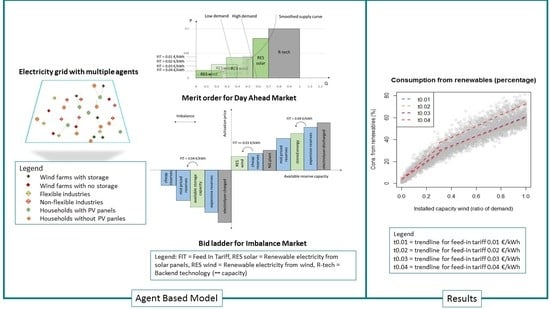
2.1. Developing the ABM

Netlogo (6.0.2, Northwestern University, Evanston, IL, USA) [36] was used for modelling the electricity grid for this paper. ODD + D protocol is followed to ensure comprehensiveness when reporting ABMs as it ensures that the description of the main theories and underlying assumptions in the model are clearly explained [35,37]. In this section, the parts of ODD + D that are included consist of Purpose; Entities, state variables and scales; Process overview and scheduling. The sections on Design concepts; Initialization; Input data; and sub-models are provided in Appendix A.

2.1.1. Purpose

The model has been designed for generating data to test the hypotheses that increased τ, increased ∆x and demand flexibility from industries result in more inclusion of renewable power in the grid and lowered market prices.

2.1.2. Entities, State Variables and Scales

The electricity grid modeled in this paper consists of three main agent groups; the electricity producers that are the wind farms, the large electricity consumers that are the industries, and the Small and Medium sized Consumers (SMCs) that are the households and small businesses. All of the agents are connected to the grid, which is operated by a grid operator, who ensures that the grid frequency is kept stable by reducing the mismatch between the supply and demand to zero. This system needs an efficient information and communication technology support. However, the technical details of the smart grid are beyond the scope of this article.
The model runs with quarter hourly time steps over a period of one year. The electricity grid is modeled as an island (thus, imbalance is zero), where the connections to markets or production systems outside of the model do not exist. The system parameters and the state variables are provided in Table 1. The parameters and variables that are agent dependent are detailed in Appendix A (see Table A1).
Literature supports that fewer actors providing flexibility increases the likelihood of power they can exercise in defining the market price [38]. To avoid this, it was also assumed that the size or capacity of the actors does not limit their ability to participation in either of the two markets. The properties of the agents are further described in the section below.
a. 
RES-E producers (2 groups)
The large RES-E producers are modeled as onshore wind farms, with each turbine of an average capacity of 2 ± 0.4 MW and an average rotor diameter of 80 ± 20 m and a Levelized Cost Of Electricity (LCOE) of 0.053 €/kWh (for year 2017) [39]. LCOE is defined as the cost to produce 1 MWh of electricity with a given technology is the sum of the annualized investment costs, the fuel costs, the operational and management costs and the carbon costs [40].
The on-shore wind farms were selected over the offshore ones because their LCOE is comparable to the other technologies modeled in the ABM [39]. All RES-E producers can sell the produced electricity to the electricity markets. The profit of the RES-E producers is a function of subsidy, operating cost, and the market price in a particular moment. The market for selling electricity is chosen based on the difference between the nominated supply and actual supply. If the actual supply is less than or equal to the nominated supply, DAM price is used for profit calculation. However, if the actual supply is more than the nominated supply, the extra production is placed on the IM and the IM price is considered for profit calculation, if their provided reserves are engaged on IM. At the start of the model run, all RES-E producers are randomly assigned a production strategy, which divides them into two strategic groups:
  • Non-storing producers: RE producers who do not own storage but in cases of grid imbalance can curtail their production.
  • Storing producers: Storing RES-E producers who can store electricity when the actual supply exceeds nominated supply. They provide the stored electricity and the available storage capacity as reserves on the IM.
b. 
Large industries (4 groups)
The large consumers are grouped under the category of industries. All the industries are modeled to produce one unit of product per kWh of electricity consumed. The price of one unit of product is assumed to be 1€. Each industry has a smart metering system; hence, information of their own nominated and the actual consumption is available to all industries in real time. Each of the industries has a maximum capacity of 50% flexibility in their electricity consumption. However, they are divided into four groups, three provide reserves on the IM, while the fourth group does not. The bidding prices for each group are hypothesized and are based on the relative LCOE of other technologies that are included in the study, so that the bidding price of the most expensive reserve is not above the most expensive technology (modeled as an electrolyzer) and the price of the cheapest reserves is lower than the LCOE of wind (without subsidy). The groups are labelled as following based on their strategies:
  • Group 0—non-flex: Industries that do not engage in the IM.
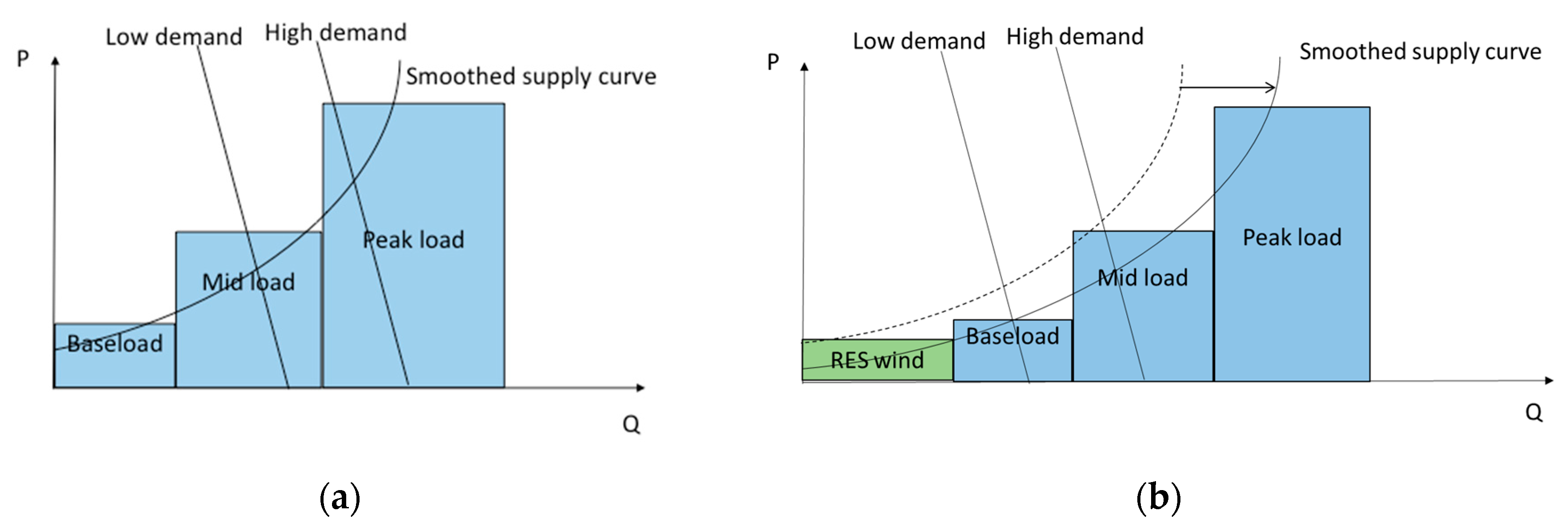
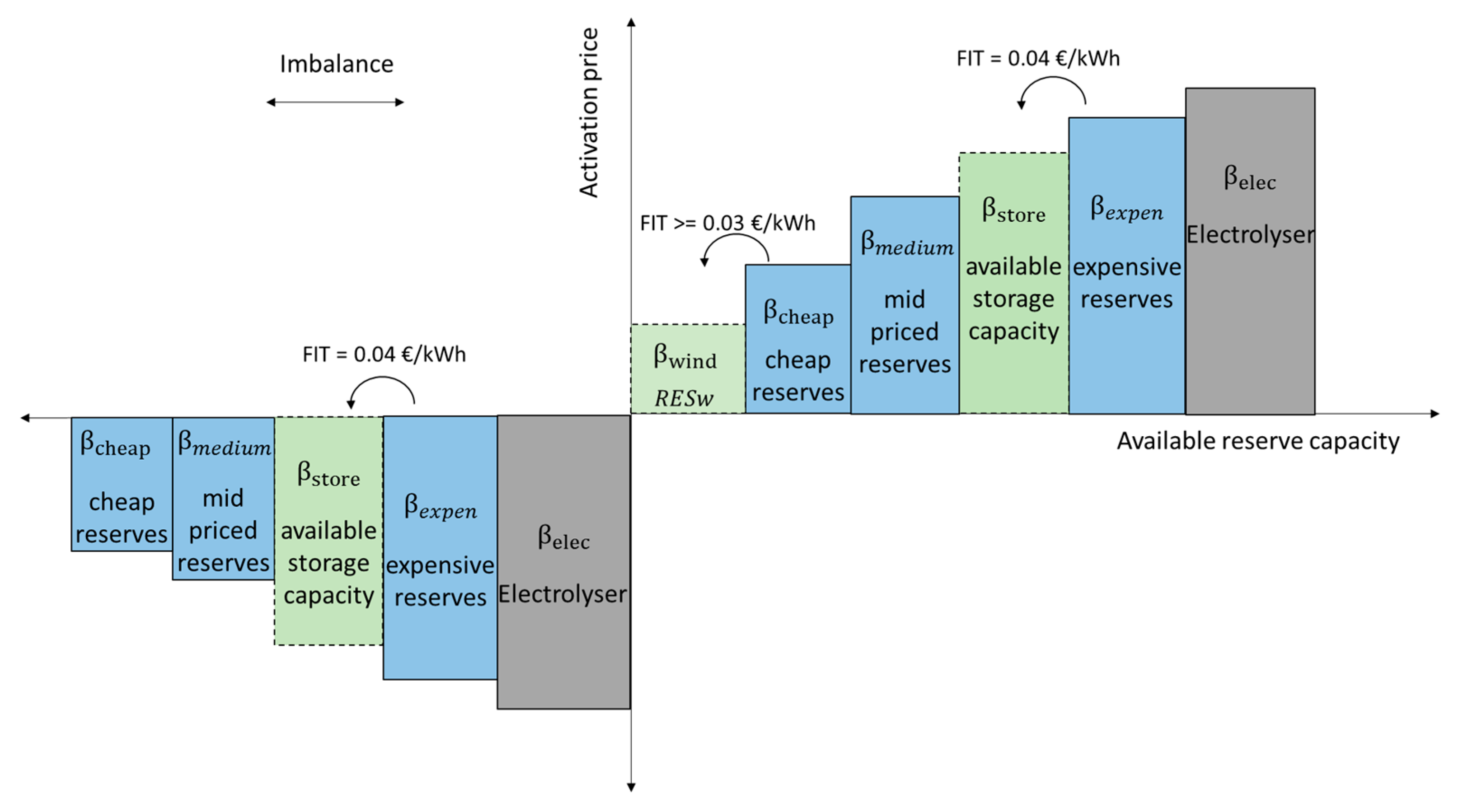
  • Group 1—cheap reserves: industries that provide reserves at a symmetric price of 0.04 €/kWh.
  • Group 2—mid-priced reserves: industries that provide reserves at a symmetric price of 0.08 €/kWh.
  • Group 3—expensive reserves: industries that provide reserves at a symmetric price of 0.14 €/kWh.
c. 
Small or medium sized consumers (SMCs) (2 groups)
The households make up this agent group. They are defined by an average electricity consumption of 12 ± 1 kWh/day, which is the average consumption of a European household [41]. The consumption pattern of SMCs depends on the time of the day. Each agent in this group is charged with a bill at the end of the year for the amount of electricity that they consume. Half of the consumers also have Photovoltaic (PV) panels and are hence termed prosumers. The electricity produced by prosumers is first used to meet own demand and the extra is placed on the grid. However, if there is no demand for this electricity, the grid operator can decide to cut the injection of electricity from prosumers. The prosumers do not receive the profit for injecting electricity in the grid because it is assumed that the cost of smart meters and the grid operational costs will balance the profit that the prosumers may gain. In the model, this electricity is placed by the TSO on the DAM with a price of 0.08 €/kWh, which is the LCOE of a PV [42]. The prosumers pay a fee for getting access to the grid. In Flanders (Belgium), it is an annual flat fee of 85 €, which is also used in this model to calculate the bill of the prosumers [43]. In the model, the SMCs fall into following two categories based on their strategies:
  • Prosumers: SMCs with PV panels,
  • Consumers: SMCs without PV panels.
All SMCs receive the bill at the end of the year, which is calculated by considering the annual average price of both electricity markets. In case of the prosumer, the self-consumption is billed as 0.
d. 
Electricity markets
There are two market environments modeled; DAM and IM. In the ABM, all technologies that participate in the market are ranked according to their LCOEs.
An inflexible base load (abbreviated as fixed-prod) is assumed to provide 20% of the average system consumption at an LCOE of 0.02 €/kWh, comparable to the cost of a hydro power plant in Europe [44]. 10% of the average system consumption is provided by the flexible or interruptible gas fired power plant (NG plant) at a cost of 0.04 €/kWh [40]. The renewable energy capacity from the RES-E producers (RES-wind) is modeled to match at least 25% and at maximum a 100% of the average demand of the system. Half of the SMCs are also modeled to own PV panels, the capacity of which as determined to meet the SMC’s own average demand per annum. The electricity that is put on the grid by the SMCs is termed as RES-solar.
On the DAM, the consumers and producers nominate consumption and production capacity, respectively, for the next 24 h. The match between the supply and demand defines 24 values of the market price on the next day. This is done based on the merit order of cheaper to expensive technologies that are engaged to provide the supply. In case of limited supply and a DAM price higher than 0.1 €/kWh, it is assumed that a backup technology (R-tech) is used to provide the necessary electricity and ensures that the market price does not rise further and the system remains stable. The price of buying electricity from the backup technology is a constant 0.1 €/ kWh. Since consumption defines how much supply will be engaged and never the other way around, the price of DAM never drops below the price of the cheapest technology. It also ensures that the DAM price never rises above 0.1 €/kWh. The merit order of these technologies from the cheapest to the most expensive is shown in Figure 3.
Increasing levels of RES-wind capacity and RES-solar are expected to stabilize the DAM price at a lower value. However, in the case of low demand, this increased production capacity may lead to a surge in the injection and would require to be settled in the IM. The IM is a quarter hourly market and hence operates to balance mismatch between supply and demand at a time scale of fifteen minutes. The default value for IM price is 0 €/kWh, unless the demand or supply deviate from their day ahead nominations, causing an imbalance. The former triggers a downward activation, which means that the reserves are requested to decrease consumption or an upward activation from the RES-E producers is required. The agents who engage in the IM are the industries who provide reserves and the RES-E producers. The other technologies in IM consist of a flexible Natural Gas (NG) fired power plant with a bid price of 0.04 €/kWh, and an electrolyzer with a symmetric bid price of 0.2 €/kWh. The merit order of these reserves is provided in Figure 4.
The model includes a number of parameters for the agents, technologies, and the market environments that have been explained above. In addition, during the simulation runs, the flow of electricity and money between the agents is governed by different variables that again define the state of the agents, technologies, and the market environments. While Table 1 provides the information for the technologies and the market environment, the detailed information about the agents can be found in the annex (see Table A1).
For the data on wind velocity and solar irradiation, the database of Belgian Electricity Transmission System Operator, Elia was used [47]. The data on wind velocity and solar irradiation are not meant to depict the exact values but create a realistic pattern of wind speed and solar irradiation in a year for Belgium. More information on how these data were acquired and how the wind power and solar power are calculated is provided in the annex.

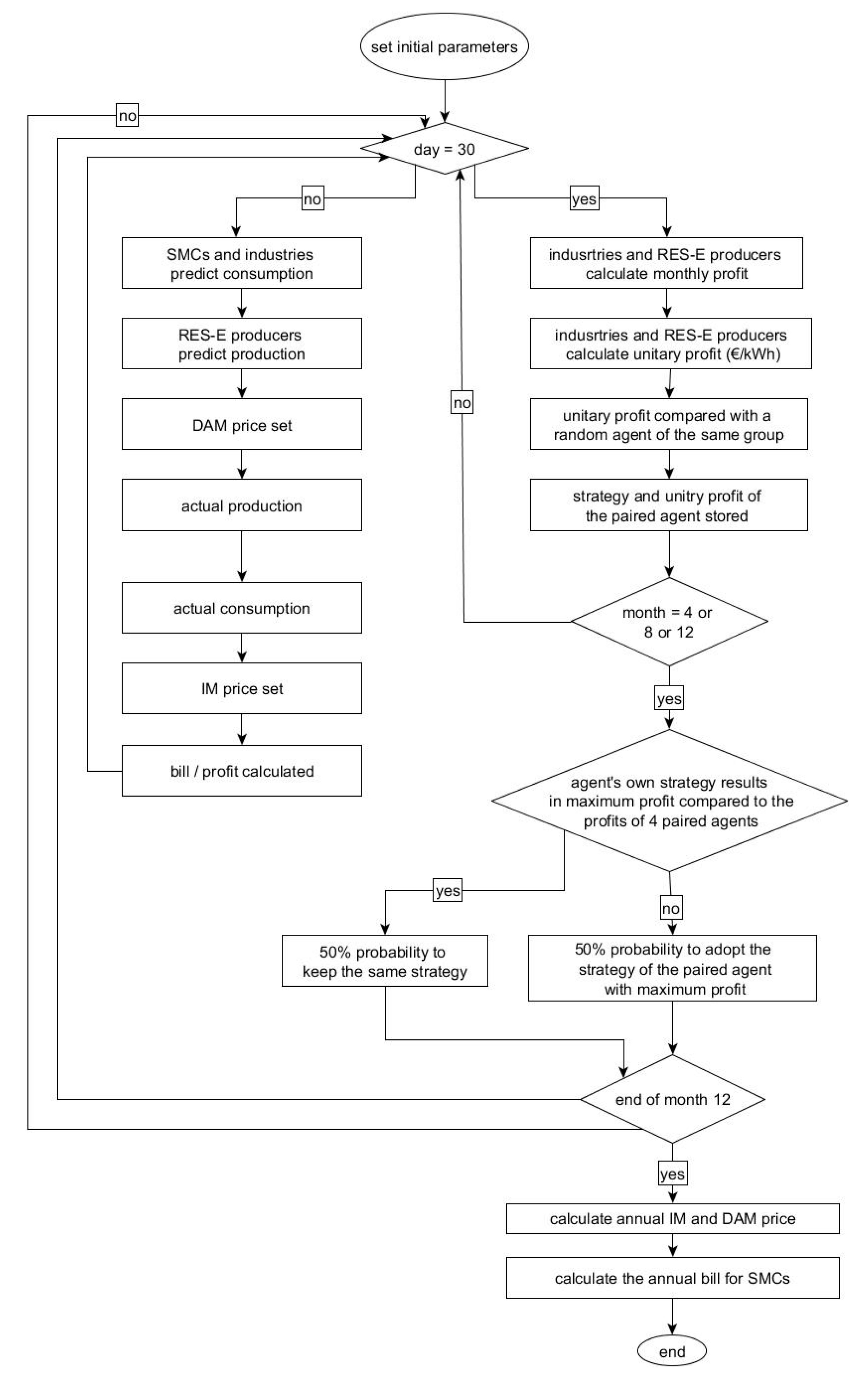
2.1.3. Process Overview and Scheduling

The sequence of actions for the model is depicted in Figure 5.
After the model has been set up, the model is run in the following order:
  • Predicting consumption and production for the next day,
  • Setting a DAM price for each hour of the day,
  • Actual consumption and production in every quarter,
  • Calculating the system imbalance to decide to engage the IM,
  • Based on the imbalance, setting the IM price for every 15 min,
  • Updating the system variables,
  • Calculating profit,
  • Storing the unitary profit producers at the end of every month,
  • Storing the unitary bill of SMCs and industries at the end of every month,
  • Changing behavior based on the comparison of unitary bill and unitary profit with other agents in the past three months,
  • At the end of the year, calculate the bill for SMCs.

2.2. Statistical Analysis

The two main variables in this study that were varied to test their effect on the whole system are feed-in tariffs ( τ ), and the installed capacity of wind power as a ratio of the average demand of the whole system (∆x). Both variables are treated as continuous variables with ranges of 0 to 0.04 for τ and a range of 0 to 1.00 for ∆x. Three response variables were observed in the analyses; Q R E % (percentage of system demand met by RES-E), C D A M . a n n u m (the annualized DAM price) and C I M . a n n u m (the annualized IM price). The ABM was used to run 5000 simulations to generate data that were then fitted with linear regression models using the statistical program R [48]. All statistical tests were two sided and had a significance level of 0.05%.

3. Results

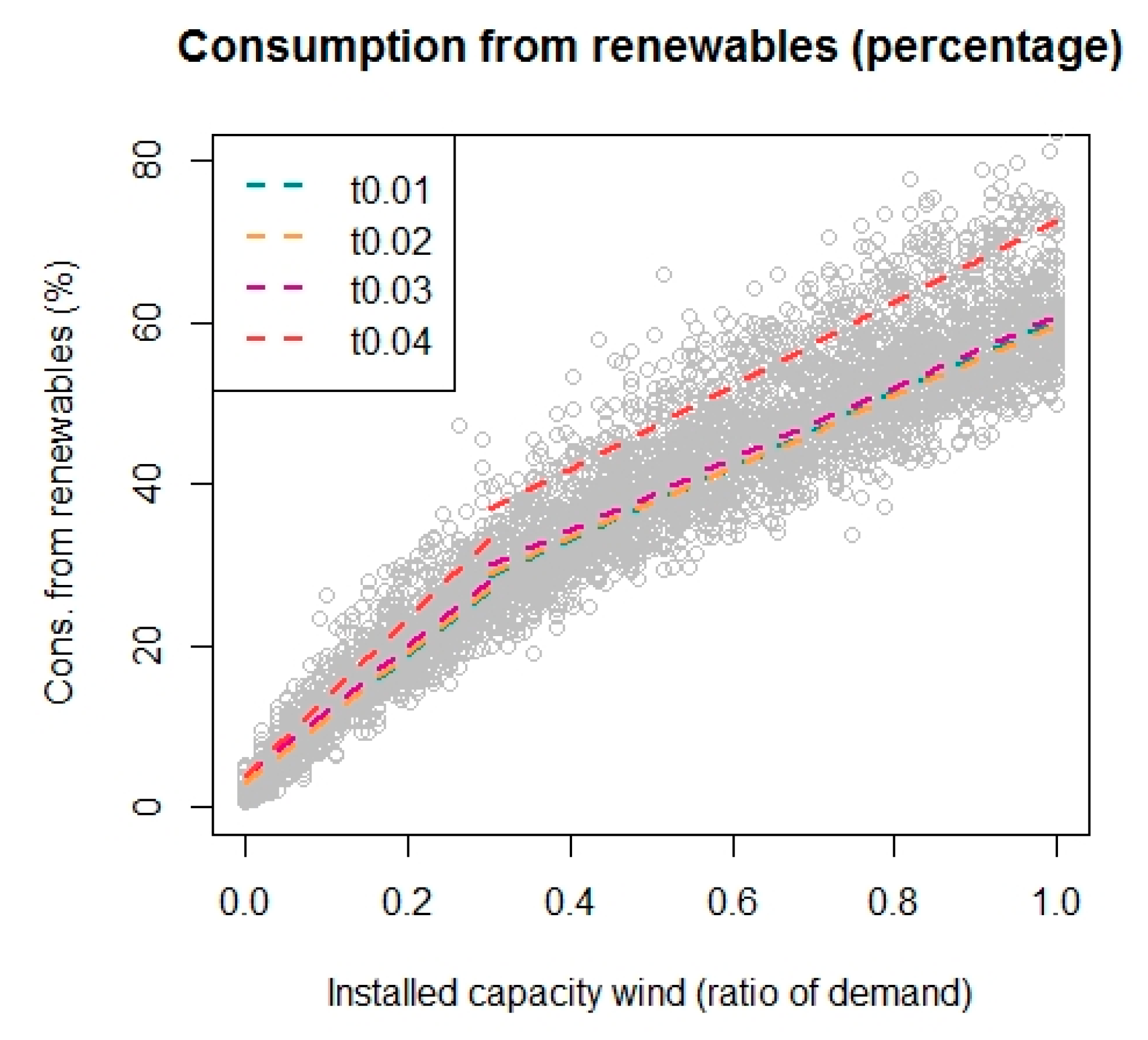
3.1. Effect on the RES-E Consumption

Figure 6 shows the mean RES-E consumption for all scenarios which is noted to increase sharply following the increase in ∆x until the installed capacity reaches 35% after which the slope becomes less steep. To explain the effect of τ and ∆x on Q R E % , the data were fitted with a linear regression model (Equation (1)).
Q R E % ^ =   8.178 + 54.958 ( Δ x ) 0.185 ( τ 0.01 ) + 0.173 ( τ 0.02 ) + 1.063 ( τ 0.03 ) + 2.373 ( τ 0.04 ) +   0.0806 ( Δ x . τ 0.01 ) 0.728 ( Δ x . τ 0.02 ) 0.476 ( Δ x . τ 0.03 ) + 11.333 ( Δ x . τ 0.04 ) .
The linear model for Q R E % explains 95% of the variations in the observed percentage of system consumption from renewable sources with a residual standard error of 4.16%. The curvature in the predictions for Q R E %   is not explained solely by the above linear equation. Hence, the data were divided into two sections with Δ x < 35 % and Δ x 35 % for further explanation. This resulted in two regression models, which are depicted by the Equations (2) and (3). The regression model (Equation (2)) explains 88% of the variations in Q R E % , with a residual standard error of 3.14% (1740 degrees of freedom). While the second model (Equation (3)) explains 83% of the variation in Q R E % with a residual standard error of 4.266% (3240 degrees of freedom). See Appendix B (Table A2) for the more detailed information on the parameter estimates for the regression models. The fitted trend line for each value of τ for each regression model is shown in Figure 6:
When Δ x < 35 % ,
Q R E % ^ = 3.315 + 77.813 ( Δ x ) 0.374 ( τ 0.01 ) 0.285 ( τ 0.02 ) + 0.562 ( τ 0.03 ) + 0.424 ( τ 0.04 ) + 1.846 ( Δ x . τ 0.01 ) + 2.328 ( Δ x . τ 0.02 ) + 2.710 ( Δ x . τ 0.03 ) + 20.180 ( Δ x . τ 0.04 ) ,
When 35 % Δ x 100 % ,
Q R E % ^ = 15.701 + 44.560 ( Δ x ) 0.646 ( τ 0.01 ) + 0.118 ( τ 0.02 ) + 1.134 ( τ 0.03 ) + 5.742 ( τ 0.04 ) + 0.670 ( Δ x . τ 0.01 ) 0.700 ( Δ x . τ 0.02 ) 0.618 ( Δ x . τ 0.03 ) + 6.697 ( Δ x . τ 0.04 ) .
When the maximum ∆x is less than 35%, the increase of every 10% in ∆x in the absence of any feed-in tariffs will result in an increase of 7.7% in Q R E % . The regression lines (t0.01, t0.02, t0.03, and t0.04) show the effect of feed-in tariffs (Figure 6). When ∆x is increased by 10%, it results in 3.4, 5.0, 6.5, and 9.1% increase in Q R E % , until ∆x reaches 35%. Equation (3) shows a less steep slope in predictions for Q R E %   as ∆x increases from 35% to 100%. It shows that, in the absence of feed-in tariffs when ∆x increases by 10%, it results in an increase of 4.4% in Q R E % . In addition, the effect of feed-in tariffs at 0.01, 0.02, 0.03, and 0.04 €/kWh results in a respective increase of 4.5, 4.3, 4.3, and 5.1% in Q R E % for every 10% increase in the value of ∆x until it reaches 100%. This analysis shows that the increase in ∆x is the main factor that affects the increase in Q R E %   as compared to increasing values of τ .
Conclusively, the statistical analysis shows that there is not enough evidence to reject that there is no significant effect of τ and the ∆x on the consumption of renewable energy (p-value < 2 × 10⁻¹⁶). In fact, both factors result in increasing the consumption from RES-E, with the most rapid increase observed when feed-in tariffs for RES-E producers are provided at a value of 0.04 €/kWh while the installed capacity of wind power is between 0 and 35%.

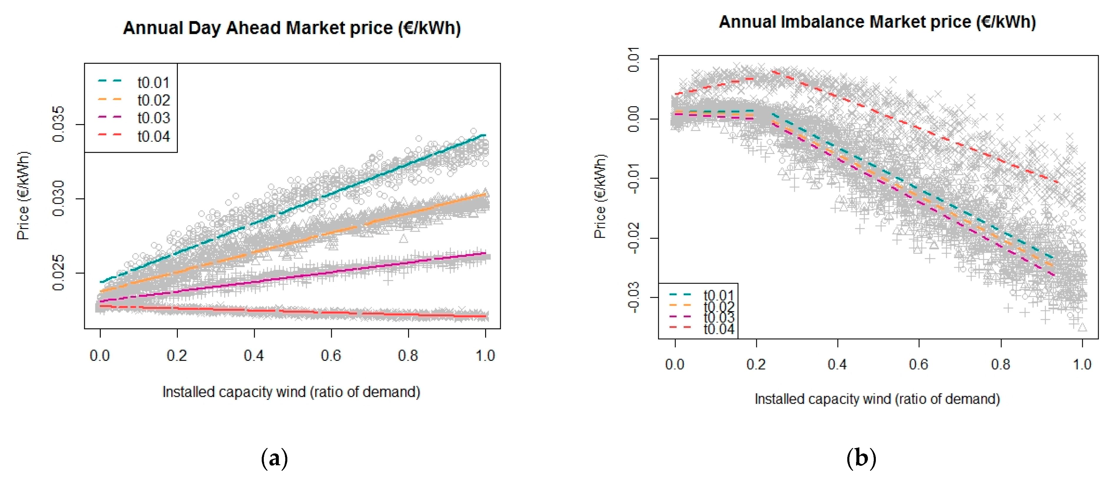
3.2. Effect on the Market Prices

The two market prices dictate the profits of the industries and the producers and the bill for the SMCs in the system, hence the factors that affect the market prices influence all the agents in a direct or an indirect manner. The two graphs in Figure 7 show the effect of τ and ∆x on the two market prices. For DAM, the four tariff levels show a significant effect as the ∆x is increased. The four trend lines for each value of τ are shown in Figure 7a, while the linear model from where these trend lines are acquired is given in Equation (4). See Appendix B (Table A2) for the more detailed information on the parameter estimates for the regression model.
When the data observed for annual DAM prices were fitted in a linear regression model (Equation (4)), it showed significant effect of τ and ∆x. The regression model for DAM prices explains 97% of the variation in the annualized DAM prices with a residual standard error of 0.0006169 (4990 degrees of freedom). See Appendix B (Table A2) for the more detailed information on the parameter estimates for the regression model. The regression model predicts that, under the sole effect of increasing ∆x, the annualized DAM prices will increase by 0.01 €cents/kWh for every 10% of increase in ∆x. From the four trend lines in Figure 7a, it is derived that, for 10% of increase in ∆x and feed-in tariffs at 0.01, 0.02, and 0.03 €/kWh, a respective increase of 0.09, 0.06, and 0.03 €cents/kWh can be expected in the mean annualized DAM price—while a feed-in tariff of 0.04 €/kWh provided to the RES-E producers can result in a decrease of 0.0007 €/kWh in the mean annualized DAM price with every 10% of increase in ∆x until it reaches 100%:
E [ C D A M . a n n u m ] ^ =   0.002 + 0.001 ( Δ x ) 0.0006 ( τ 0.01 ) 0.001 ( τ 0.02 ) 0.001 ( τ 0.03 ) 0.0002 ( τ 0.04 ) 0.003 ( Δ x . τ 0.01 ) 0.006 ( Δ x . τ 0.02 ) 0.010 ( Δ x . τ 0.03 ) 0.013 ( Δ x . τ 0.04 ) .
The data for annualized IM prices shown in Figure 7b show an increase in the IM prices until ∆x is above 25%, after which the data show a downward trend. Therefore, we divided the data into two parts and fitted separate regression models to them to explain the pattern that is followed by the IM prices. The linear regression model in Equation (5) explains the 72% of the variations in the IM prices when Δ x < 25 % , with a residual standard error of 0.001266 (1240 degrees of freedom). Equation (7) explains 87% of the variations in the IM prices when 25 % Δ x 100 % , with a residual error of 0.003329 (3740 degrees of freedom). See Appendix B (Table A2) for the more detailed information on the parameter estimates for the regression models:
E [ C I M . a n n u m ] ^ =   0.0062 0.029 ( Δ x ) 0.0004 ( τ 0.01 ) 0.0009 ( τ 0.02 ) 0.001 ( τ 0.03 ) + 0.003 ( τ 0.04 ) 0.001 ( Δ x . τ 0.01 ) 0.002 ( Δ x . τ 0.02 ) 0.03 ( Δ x . τ 0.03 ) 0.009 ( Δ x . τ 0.04 ) .
The trend lines that are added to the graphs are indeed acquired from these main equations. It is visible in Figure 7b that t0.01, t0.02, and t0.03 have an almost equal slope, whereas t0.04 has a steeper slope in the first part of the graph and a smoother slope in the second part of the graph. Equation (6) shows that, in the absence of feed-in tariffs, with a 10% increase in ∆x, the annualized IM prices will increase by 0.03 €cents/kWh. This is due to the fact that, when there is less wind power being produced, the RES-E producers cannot offer large volumes of power on DAM, resulting in deficit of supply. Hence, when IM prices also spike, RES-E producers (storing and non-storing) cannot offer much to balance the grid. This results in more expensive reserves being engaged on IM. In addition, when the feed-in tariff of 0.01 €/kWh is provided to the RES-E producers, it results in little effect on the position of RES-E producers in the bid ladder, and only results in increasing the IM prices by 0.004 €cents/kWh for every 10% increase in ∆x.
For feed-in tariffs of 0.02 and 0.03 €/kWh, the RES-E producers move to a second spot on the merit order list for DAM. This leaves less reserves from RES-E producers being made available for IM. This shift of positions in the merit order causes more power being offered as supply (to compensate for the unpredictable nature of wind). This results in a decrease in IM prices by 0.033 and 0.044 €cents/kWh, respectively. Furthermore, when feed-in tariff of 0.04 €/kWh is provided to the RES-E producers, it moves their position to first in the DAM bid ladder. This results in more volumes being made available for DAM from all RES-E producers. This leaves almost no stored reserves available for the IM, which results in engaging more expensive reserves and ultimately increasing the IM prices.
When Δ x < 25 % ,
E [ C I M . a n n u m ] ^ =   0.001 + 0.0031 ( Δ x ) 0.0001 ( τ 0.01 ) 0.00005 ( τ 0.02 ) 0.0003 ( τ 0.03 ) + 0.0028 ( τ 0.04 ) 0.002 ( Δ x . τ 0.01 ) 0.006 ( Δ x . τ 0.02 ) 0.007 ( Δ x . τ 0.03 ) + 0.011 ( Δ x . τ 0.04 ) .
When 25 % Δ x 100 % ,
E [ C I M . a n n u m ] ^ =   0.009 0.034 ( Δ x ) 0.0007 ( τ 0.01 ) 0.001 ( τ 0.02 ) 0.001 ( τ 0.03 ) + 0.004 ( τ 0.04 ) 0.0005 ( Δ x . τ 0.01 ) 0.0007 ( Δ x . τ 0.02 ) 0.002 ( Δ x . τ 0.03 ) + 0.008 ( Δ x . τ 0.04 ) .
This trend in IM price changes once Δ x is increased above 25%. This results in decreasing the IM prices as Δ x increases, with and without the provision of feed-in tariffs. In the absence of τ , every 10% increase in Δ x results in a decrease of 0.03 €cents/kWh. It is simply an effect of extra volume of electricity being produced by the RES-E producers when there is no demand. The trend lines in Figure 7, derived from Equation (7), exhibit that, with every 10% increase in Δ x until it reaches 100%, the IM price decreases by 0.034, 0.035, 0.036, and 0.026 €cents/kWh, respectively, when feed-in tariffs are 0.01, 0.02, 0.03, and 0.04 €/kWh. Other than the decrease in IM prices in relation to increasing Δ x , it is also worth noting that the mean IM prices remain higher when a feed-in tariff of 0.04 €/kWh is provided to the RES-E producers. This is again an effect of the all electricity volumes being made available for DAM, leaving no predicted volumes for storage on the next day. This results in, firstly, too much supply (hence negative IM prices) and, secondly, no stored electricity reserves (hence more expensive reserves being engaged).
The statistical analyses presented above show that there is not enough evidence to reject the second hypothesis of the study and there is a significant effect of τ and the ∆x on the two market prices (p-values < 2 × 10⁻¹⁶).

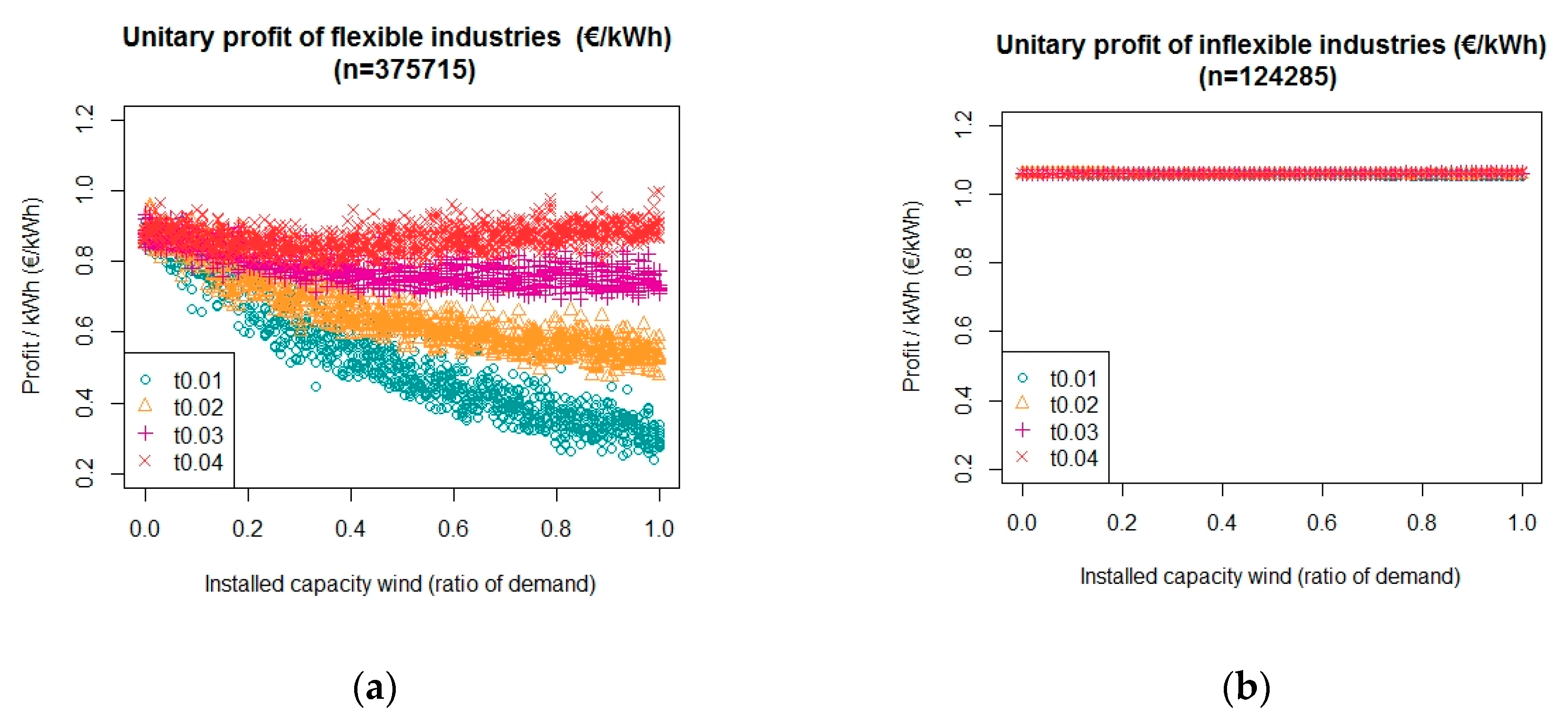
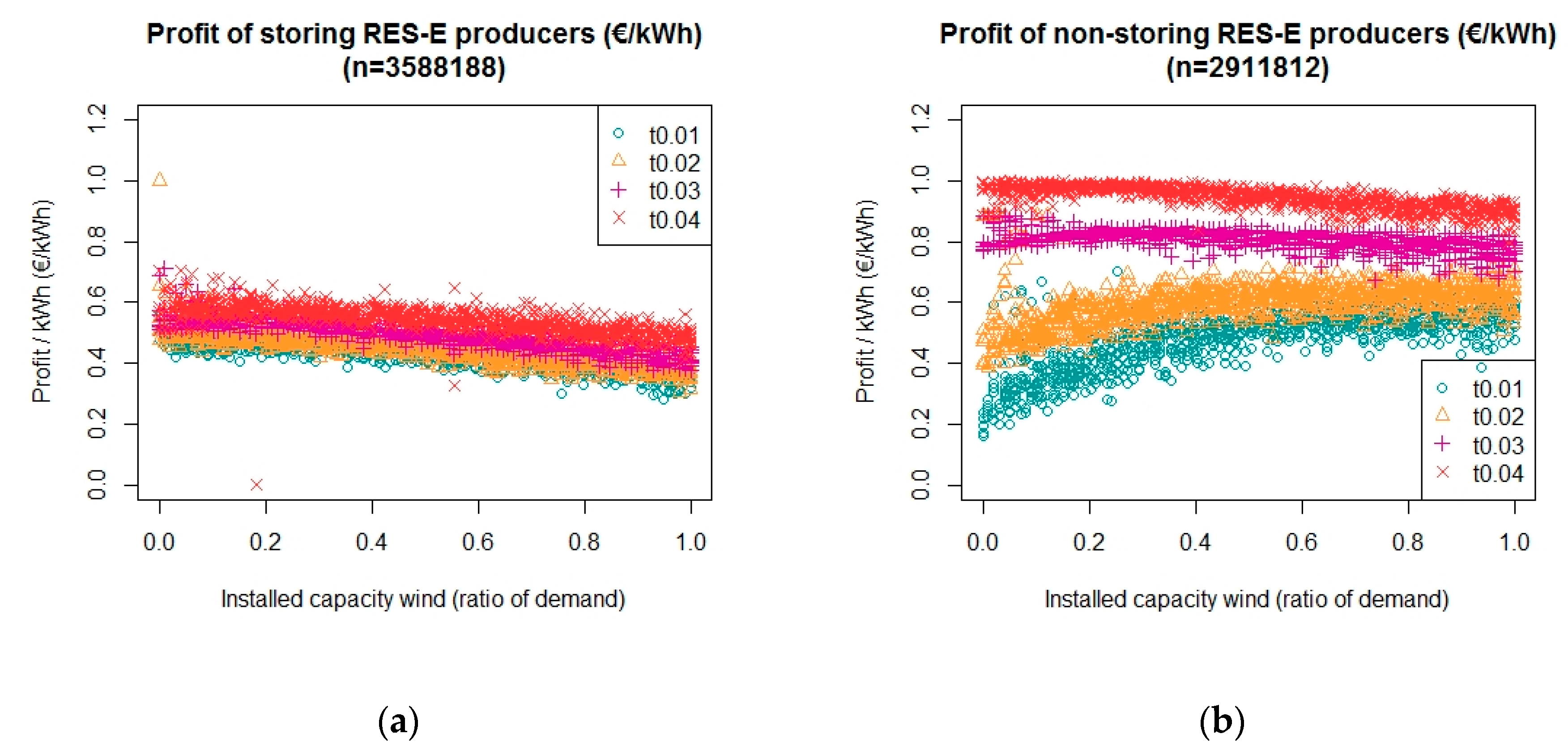
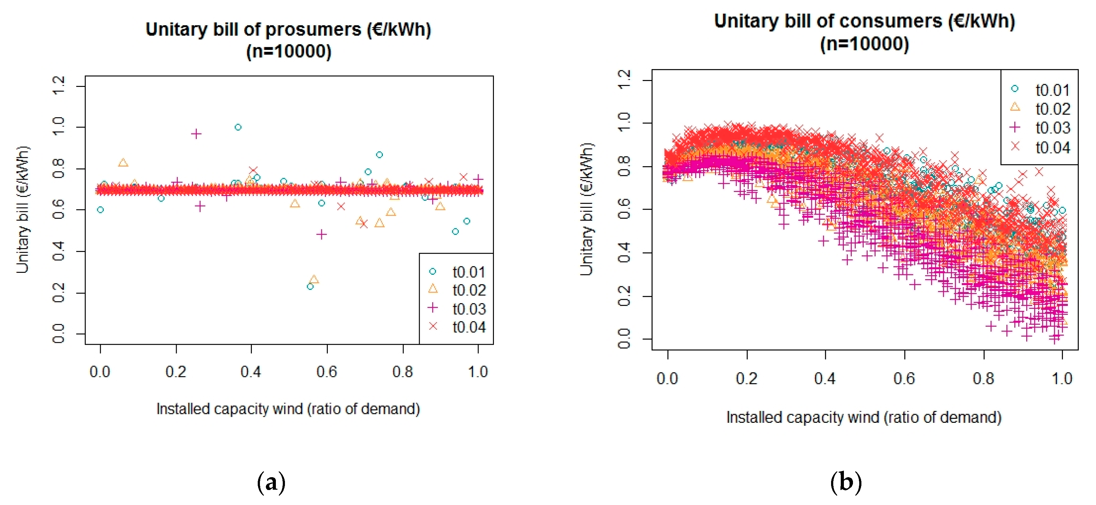
3.3. Effect on Different Agents

Graphs (a,b) in Figure 8 show the mean unitary profits for the two industry groups different feed-in tariffs and increasing Δ x . It is evident that, with increasing Δ x , the unitary profits of flexible industries, who engage in the IM, increase when τ is 0.04 €/kWh. For all other values of τ , the mean profits of flexible industries decrease with increasing Δ x . This effect is owed to the modelling method of flexible industries, who always respect their nominated consumption pattern. This results in them paying the bill, which is heavily dictated by the DAM price. Thus, as the DAM price decreases, the profit of flexible industries increases. Although flexible industries respond to demand changes according to the imbalance on the grid, the IM bidding prices are not as high to compensate for the production losses. However, the unitary profit of the inflexible industries (which do not participate in IM and do not respect their nominated consumption) shows no variation as a response to increasing feed-in tariffs and installed capacity of wind power. The more selfish consumption of electricity results in a very stable profit for the inflexible industries. However, in reality, such deviations from nominated power can result in fines for large consumers.
The effects of the τ and ∆x were also assessed for impact on the profits of the two producer groups separately. Figure 9a shows the mean unitary profits of storing RES-E producers, where the variation between the different simulations is very narrow and the effect of different feed-in tariffs does not appear to cause a pronounced variation in the profits. However, the general trend that can be observed from this figure is of decreasing profits as the installed capacity of wind increases. On the contrary, Figure 9b shows higher mean unitary profits of the non-storing agents. The most interesting conclusion from the graphs in Figure 9 is that the overall mean profit of non-storing agents is higher than the storing RES-E agents. In addition, increasing ∆x negatively affects the profit of storing producers, while it increases the profit for non-storing agents when τ is 0.01 and 0.02 €/kWh but results in a decreasing profit as ∆x increases for a value of 0.03 and 0.04 €/kWh for τ . The simple reason is the decreasing profits of storing and non-storing RES-E producer (only under τ of 0.02 and 0.03 €/kWh) is the extra volumes of wind power being made available on the grid, while the demand does not increase accordingly.
The numbers on top of Figure 9a,b show the number of storing and non-storing RES-E producers at the end of the simulation runs. It shows that the number of RES-E storing producers is almost double the number of RES-E non-storing producers. Due to the adaptation function, modeled in the ABM, it shows that more RES-E producers chose to have storage, as it would have prevailed as a more profitable strategy during the simulation runs. At the start of every simulation run, the number of RES-producers is modeled to be random with an equal chance of any RES-E producers appointed storage facilities. This effect could be a result of lower operating costs for the RES-E producers and hence a higher chance of being engaged on DAM (first position in the bid ladder) and IM (first position for non-stored electricity and fourth for the stored power).
Finally, the mean unitary bill for households with PV panels and without being in relation with increasing values of ∆x is shown in Figure 10. Comparison of Figure 10a,b shows that the mean bill of SMCs follows the same pattern as the market prices. When the mean bill of consumers is separated according to the ownership of PV panels, it suggests that it is, in fact, not very profitable for households’ own PV panels when the installed capacity of wind energy is above 50% of the average system demand, as compared to the households without PV panels. There are two factors that cause disparity between the bill of the prosumers and consumers; first, the amount of consumption of electricity from the grid, and, second, the effect of the prosumer tariff. The very limited variation in the bill of the prosumers is a result of their limited reliance on the grid to fulfill their needs, which results in almost no effect of the market prices on their unitary bill, as compared to the consumers who rely solely on the grid for the electricity supply.

4. Discussion

Negative market prices for electricity are a rare phenomenon. In our results, the IM prices fall below zero with increasing values of ∆x above 25%. In reality, the European energy grid allows the grid imbalances to be reduced from the different countries, while, in this model, the grid is modeled as a stand-alone system, hence negative values on IM are observed more frequently than in reality.
From the results, it is obvious that the two market prices are decoupled, where the DAM prices remain significantly higher than the IM prices. This is a result of how the markets were modeled, allowing for the wind farm owners to bid their extra capacity on the IM. The authors in [23] mentioned that, if capacity bids from RES-E are in use on the reserve market, the energy price on reserve markets may get lower than on the intra-day market, creating distorting incentives. It shows the ability of the presented ABM to depict the working of the electricity markets.
The decreasing market prices in the simulations as a result of the increasing installed capacity of wind energy have also been observed in Germany. The authors in [49] have shown that, on the German market, each additional GWh of RES-E fed to the grid has resulted in lowering the spot market price of electricity by $1.4–1.7/MWh. The authors in [50] found that the negative prices on the DAM and IM in Belgium, Germany, and France occur due to low consumption demand and high RE generation expectation; one of the reasons is the current support mechanisms for solar and wind power [6]. Conversely, it can be argued that decreasing the feed-in tariffs and increasing the installed capacity of wind energy may result in deteriorating the profit of the RES-E producers. This only stresses that, once the subsidies are taken away, there is a need for different rules for the flexible RES-E producers to support their participation in the market and increase the supply of RES-E.
Developments in the power electronic technologies have made the application of energy storage systems a possible solution for modern (flexible) power application [51,52]. It also has been shown that battery-based energy storage with several minutes of run time is optimal for stabilizing wind generation in weak grids [53]. However, these systems are still not economically viable for the wind farm producers, as shown in the low profits for the storing agents.
It needs to be mentioned that, since the average of the two market prices is considered for billing the SMCs, the bills do not reflect reality. In reality, the supplier would nominate the consumption on the market for the consumers under a contract and the consumers will be billed according to the mismatch from these nominations. The average bill for the SMCs exhibits an opposite trend to what was observed in Germany, where the electricity price increased by 30% from the year 2006 to 2012, while the average household income grew by 6% [54]. To improve the accuracy of the bill for the SMCs, it will be useful to include the service as well as the grid operation charges in the calculation of the bill.
In the simulation results, the very pronounced effect of feed-in tariffs for the RES-E producers on the market prices points to the need to include more power production technologies in the model, which will also reflect reality. One such technology could be dispatchable renewables, such as biomass. Authors in [55] suggested that, for a power system completely based on renewables, these technologies can be incentivized to increase flexibility. Whether it is more effective to incentivize wind farm owners so they can compete with other technologies or rather provide incentives to dispatchable renewables that can replace the fossil-fuel based systems could be another topic to use the presented ABM.
For businesses, the decision to provide flexibility as a reserve is complex and can result in major organizational and operational changes. In the model, the industries responded to supply changes regardless of the time of the day and neither did they consider any lead times; in reality, though, this is probably not the case. Although the simulations provide insightful results regarding industries’ electrical flexibility as reserves, these results are not extended to other issues. For example, there are legal issues involved when industries plan to market negative tertiary reserve energy in small amounts because of tight storage restrictions [56]. Another reason to keep the industries from providing flexibility as demand response could lie in the relatively low energy price that they pay (as compared to other costs) and could be mitigated by policies opposite to the ones in practice that subsidize heavy industries [57]. Other incentives for energy intensive industries to reduce their energy costs lie in their ability to install combined heat and power plants. The authors in [58] assessed in detail the benefits for industries to engage in symbiotic relations and utilize waste (biomass) to fuel combined heat and power plants. One can argue in favor of such practices against consumption flexibility, especially if it does not incur changes in business as usual.
Finally, the complexity of a flexible electric grid poses a challenge to the diffusion process of flexibility [59]. Flexibility in consumption and production of power requires a longer time to be successful and completely diffused as an important component of the social aspect of the power system. It will require changes in human behavior and institutional setup; both domains with high inertia towards change [57]. One example of this phenomenon, termed response fatigue, occurs when the consumers tire of continuously responding to supply (and/or market price) signals. This behavior was reported in [60], with up to 98% of the residential consumers who participated in a demand response program. The results of the model point to higher need for flexibility and demand response from the consumers for the increased injection of RES-E in the grid. If the households are also to be included as active participants of demand response, there is a need to provide them with awareness and information on the energy markets, next to the provision of in-home display devices that will provide them with real-time information on their consumption and market prices [10].

5. Conclusions

The objective of this article was to model the two electricity markets (day ahead and imbalance market) by using Agent-based Model (ABM) and assess two hypotheses. The first hypothesis was to test the effect of increasing feed-in tariffs ( τ ) and installed capacity of wind energy (∆x) on increasing the consumption from renewables. The second hypothesis was to check the effect of the same factors on decreasing the two market prices. This objective was successfully met by using ABM to generate the data that were then fit into linear regression models to reach conclusions on the hypotheses.
The study concludes that, with increasing ∆x by 10%, the consumption from RES-E increases by 7.8% in the absence of τ , until ∆x reaches a maximum of 35%. At different levels of τ , the increasing consumption from RES-E increases differently. The most pronounced is when τ is set at the value of 0.04 €/kWh and the maximum ∆x is 35%. For ∆x higher than 35% and less than 100%, the increase in RES-E follows a less sharper increase and once again the sharpest increase is for τ = 0.04 €/kWh, which under every 10% increase in ∆x results in a 5.1% increase in RES-E consumption.
To test the hypothesis about the market prices, different regression models were fit to explain the Day Ahead Market (DAM) and Imbalance Market (IM) prices. DAM prices increase by 0.01 €cents/kWh for every 10% increase in ∆x in the absence of τ . With increasing ∆x when   τ is provided at 0.01, 0.02 and 0.03 €/kWh, the increase in the DAM prices is less sharp. In addition, with every increase in the value of τ , the mean DAM price is lowered as compared to the previous value of τ . When the value of τ is 0.04 €/kWh, it results in decreasing DAM prices as ∆x increases. The increasing values of τ enable RES-E producers to nominate more power on the DAM at lower marginal costs, thus lowering the overall DAM prices. At 0.04 €/kWh, the effect of τ is two-fold because, at this level, the storing RES-E producers can also nominate stored electricity on the DAM, while still being cost competitive. Hence, more electricity is nominated for DAM and electricity prices are lowered as a result.
The regression model to explain the trend observed in the IM prices had to be split into two further models. Briefly reported, the regression models show that, in the absence of τ , every 10% increase in ∆x results in a decrease in IM price by 0.031 and 0.34 €cents/kWh when ∆x is between 0 and 25% and between 25% and 100%, respectively. The models also showed that, until the maximum ∆x is less than 25%, the IM prices increase for the values of τ at 0.01 and 0.04 €/kWh, but decrease for τ of 0.02 and 0.03 €/kWh. When ∆x is between 25% to 100%, increasing the values of τ until 0.03 €/kWh result in lowering the mean IM price. However, at 0.04 €/kWh, the mean IM price is higher, showing the effect of no storage reserves being available on IM and more expensive reserves being engaged on the IM.
Conclusively, increasing values of τ and ∆x increase the consumption of renewable energy and decreases the market prices; with the effect of ∆x being more significant than the effect of τ . However, the effect of increasing values of both factors on the profit of storing RES-E producers is not positive, pointing to the need for customized rules and incentives to encourage their market participation and investment in storage facilities. The results support that, in the future, with more RES-E producers, different market rules may apply to the flexible RES-E and conventional generation [23].
Introducing flexibility in the power grid as a response of more renewable energy is a challenging task, as it requires institutional shift to a new way of production and consumption of electricity. Changes in consumer behavior will be crucial to this shift, which adds to the complexity of this inevitable undertaking. The approach of agent-based modelling can substantially contribute to the study of electricity production and consumption behavior, while contributing to a just distribution of costs and benefits between the different economic actors. It is worth mentioning that, though the technical details of the model for each agent can be refined to yield more insightful results, the presented ABM is capable of carrying out a detailed study of cost–benefit distribution between different agents in a grid solely fed by renewable power.
The results support that the RES-E agents do not have enough incentive to operate more efficiently when feed-in tariffs are being provided to them. There need to be other support mechanisms that promote investment in storage facilities for the RES-E producers. Market mechanisms that dictate fines for deviating from nominated power can further demotivate actors in the power generation business to switch to renewable energy technologies. The market mechanisms need to evolve to let more RES-E producers participate. Additionally, the demand side response will aid this transition. As more local balancing agents (aggregators) enter the power networks and virtual power plants are becoming a reality, smart metering would replace net metering systems. This will provide an opportunity to the consumers of all sizes to be flexible in response to production and market signals, ultimately resulting in a truly flexible grid. Depending on the specific markets and their respective mechanisms in different countries, it is up to the policy makers to incentivize the consumers to change, hence create a market pull for RES-E producers, and/or incentivize the RES-E producers to create a market push for change in the consumer behavior. Finally, although Belgian wind and solar profiles were used for the simulations, the observations from the model are transferrable to other countries where policy makers wish to incentivize renewable power.

Author Contributions

Conceptualization, A.S.M. and J.B.; methodology, A.S.M., J.B. and, S.L.; software, A.S.M. and S.L.; validation, J.B., S.L., and L.V.; formal analysis, A.S.M.; writing—original draft preparation, A.S.M.; writing—review and editing, J.B., S.L., L.V., and G.V.E.; supervision, G.V.E.

Funding

The research leading to these results has received funding from the European Union’s Horizon 2020 research and innovation program under Grant No. 679386, EPOS project (Enhanced energy and resource Efficiency and Performance in process industry Operations via onsite and cross-sectorial Symbiosis). The sole responsibility of this publication lies with the authors. The European Union is not responsible for any use that may be made of the information contained herein.

Acknowledgments

This research has benefitted from a statistical consult with Ghent University FIRE (Fostering Innovative Research based on Evidence).

Conflicts of Interest

The authors declare no conflict of interest.

Appendix A. Methodology

Table A1. Variables and parameters for the different agents.
DefinitionValuesUnit
Small and medium sized consumers
Agent properties (do not change during the simulation runs)
α S M C consumption capacity of a household [41]0.125kWh
Δ P V capacity of a photovoltaic panel [41]1–2kWh
Agent Variables (may change in every time step)
α p r e d predicted consumption for one quarter of an hour on the next day
α a c t actual consumption in real time
random.factora number generated every quarter of an hour to introduce randomness in the consumption profile of the consumers0.01–0.05
Q P V production from the photovoltaic panels in real time
α s e l f c o n s consumption from own PV panel (only for prosumers)
Q S M C production from the PV-panels in real time that is planned for the D A M . S p r e d
b i l l bill for the whole past year
b i l l u n i t per unit cost of electricity consumed in the past year €/kWh
Industry
Agent properties (do not change during the simulation runs)
α i n d average consumption of an industry2000 (±400)kWh
groupgroup number defining the strategy of the industry
Group 0: bid-cap of 0 kW
Group 1, 2, and 3: bid-cap of 50% of α i n d
0–3
Agent variables (may change in every time step)
α p r e d predicted consumption for one quarter of an hour on the next day
α a c t actual consumption in real time
α b i d for group 0, α b i d = 0
for group 1, α b i d =   Δ b i d Δ   R c h e a p
for group 2, α b i d =   Δ b i d Δ   R m e d i u m
for group 3, α b i d =   Δ b i d   Δ R e x p e n
α I M for group 0, α I M = α a c t   α p r e d
for group 1,2, and 3, α I M =   α b i d
α t o t total consumption in the past month kWh
Δ b i d bidding capacity (flexible demand)50% of α i n d kW
b i l l bill for the past month
P instantaneous profit in every time step
P u n i t unitary profit for the past month €/kWh
RES-E Producers
Agent properties (do not change during the simulation runs)
Δ p r o d average production capacity of a wind farm4000 (±100)kW
Δ s t o r a g e average storage capacity20% of Δ p r o d kW
C c u r costs for curtailing [61]0.022€/kWh
C s t LCOE 1 of battery storage [62]0.176€/kWh
strategystrategy defining if the producer will have storage or not
If 0, there is no storage facility
If 1, there is storage facility
0 or 1
Agent variables (may change in every time step)
Δ r e q ( D + 1 ) Required production per agent to meet the system demand kWh
Q n o m nominated power production for the next day kWh
Q p r o d actual power production in real time kWh
Q a c t part or all of the Q p r o d made available for the system kWh
Q c u r t curtailed power kWh
Q s t o r e d ( t ) stored power in real time kWh
Q D A M production sold at the DAM 2,   a l w a y s Q n o m kWh
Q b i d production bid at the IM 3 kWh
Q I M production sold at the IM
If, R wind > 0
Q I M = R wind   Q b i d
kWh
Q t o t Q D A M +   Q I M + Q I M . s t kWh
Q s u m total production traded in the markets in the past month kWh
Q I M . s t storage reserve engaged by IM. Value is positive when batteries are discharged, and negative when batteries are charged kWh
P instantaneous profit in every time step
P u n i t unitary profit for the past month €/kWh
1: Levelized Cost of Electricity; 2: Day Ahead Market; 3: Imbalance Market.

Appendix A.1. Sub-Models

Appendix A.1.1. Prediction of Consumption and Production

The model process begins on day = 0 and tick = 0, which depicts the hour 00:00 of a day. For the first quarter of an hour (one time step), the industries and SMCs predict consumption for the same quarter on the next day. The prosumers from the SMCs also predict the production from the PV panels, as Q P V depending on the capacity of their solar panels ( Δ P V ) . The producers calculate their production ( Q prod ) based on the weather predictions for that quarter on the next day. For all RES-E producers, Q prod is calculated as a product of their capacity ( Δ p r o d ) and the predicted weather ( w p r e d ).
Based on the strategy of the RES-E producer, the predicted production varies. For non-storing agents, it is equal to their Q p r o d , while, for storing agents, Δ r e q ( D + 1 ) and Q p r e d . s t o r e d define   Q n o m , where   Q p r e d . s t o r e d is the expected power production that will be stored, given that Q p r e d . s t o r e d does not exceed   Δ s t o r a g e . Hence, the Q nom   is based on Equations (A1) or (A3), and the value for Q p r e d . s t o r e d ( t + 1 ) is based on Equations (A2), (A4), or (A5). The conditions that define which equation is chosen for setting the values are explained below:
If   Δ r e q ( D + 1 )     Q p r o d +   Q p r e d . s t o r e d ( t ) , then
Q nom =   Q prod + Q pred . stored ( t ) ,
Q p r e d . s t o r e d ( t + 1 ) =   0 .
If Δ r e q ( D + 1 ) <   Q p r o d +   Q p r e d . s t o r e d ( t ) , then
Q nom =   Δ r e q ( D + 1 ) .
If Δ s t o r a g e   Q p r o d +   Q p r e d . s t o r e d ( t )   Q n o m
Q p r e d . s t o r e d ( t + 1 ) =   Q p r o d + Q p r e d . s t o r e d ( t )   Q n o m .
Otherwise,
Q p r e d . s t o r e d ( t + 1 ) = Δ s t o r a g e .

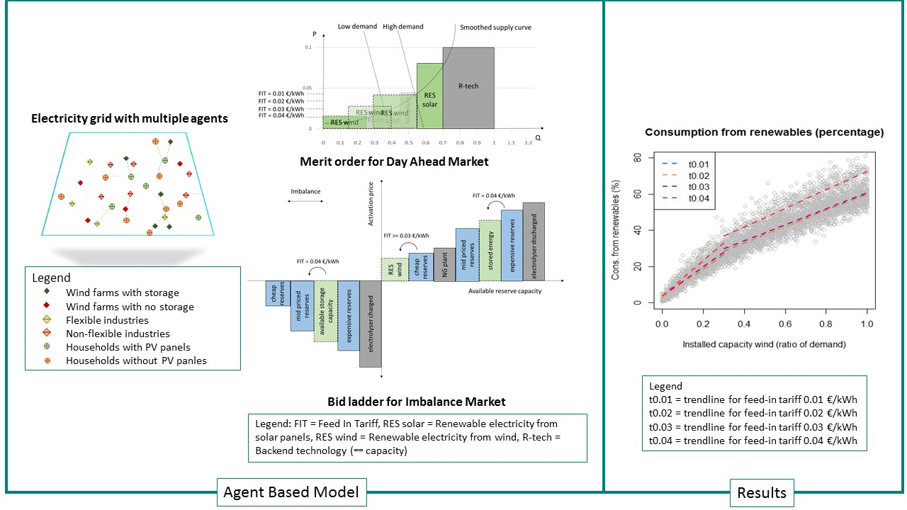
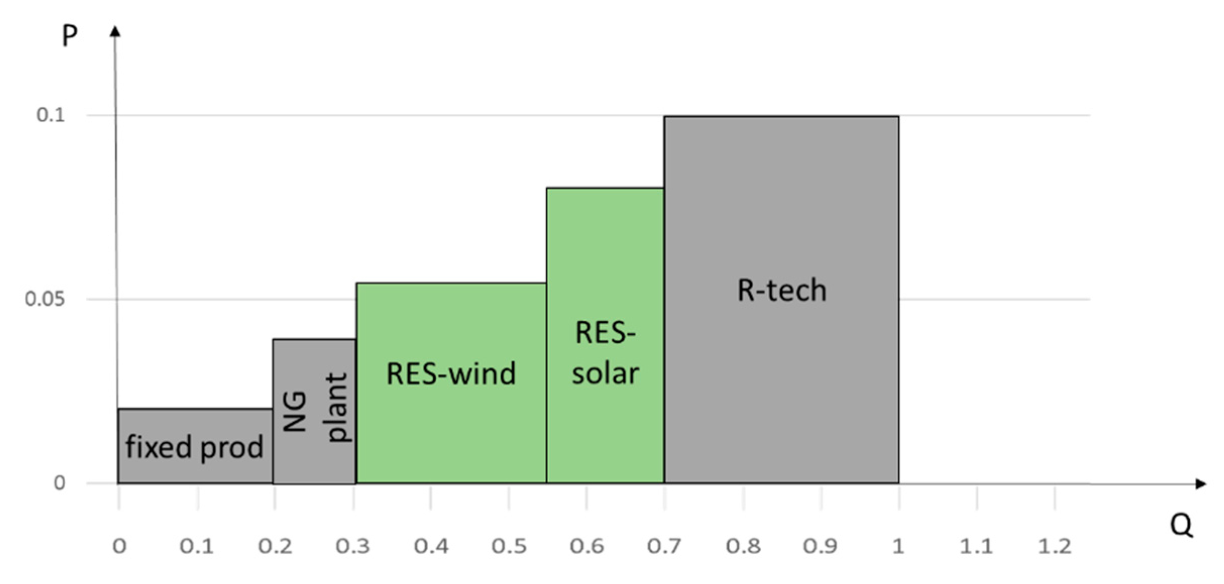
Appendix A.1.2. Setting the Day Ahead Market Price

DAM price is calculated by a merit order economic dispatch procedure. First, the total predicted demand ( D A M . D p r e d ) is calculated by summing the consumption ( i = 1 n . i n d α p r e d   + i = 1 n . S M C α p r e d )   and then matched with the available supply from different technologies arranged in order of increasing bid price.
The technology prices in ascending order are: C i n f l e x ,   C N G ,   β w i n d , C p v ,   C t e c h .
Once the supply volume is matched to the demand, the total predicted supply can be calculated as:
D A M . S p r e d = Δ i n f l e x + ( R N G Δ Δ N G ) + ( R w i n d Δ R E S . w a c t ) + ( R s o l a r Δ R E S . s p r e d ) + R t e c h ) ,
where
R t e c h = D A M . D p r e d ( Δ i n f l e x + ( R N G Δ Δ N G ) + ( R w i n d Δ R E S . w a c t ) + ( R s o l a r Δ R E S . s p r e d ) .
Since this process sets a price for every quarter, it is not representative of the DAM price. Hence, at the end of every four ticks (four quarters), the values of the last four DAM prices are averaged and one market price for the one whole hour is set. In this way on the next day, there are 24 DAM prices for each hour of the day.

Appendix A.1.3. Actual Consumption and Production

Once day 1 begins, the industries consume electricity according to the time of the day and the day of the week and their strategy. The SMCs consume electricity based on their respective profile and according to the time of the day, week of the month, and season.
For all SMCs, there consumption is a product of their predicted consumption ( α p r e d ) and a random factor.
For consumers, α a c t is the same as α c o n s
For prosumers
If α cons   Q PV
Q SMC = 0 ,
α s e l f c o n s =   | Q PV     α cons | ,
α act =   α cons   Q PV .
If α cons   Q PV
α s e l f c o n s =   α c o n s ,
Q SMC = Q PV     α s e l f c o n s ,
α act = 0 .
The consumption from all SMCs and industries ( i = 1 n . SMC + n . ind α act ) sets the value for DAM . D act
The RES-E producers produce electricity according to the weather conditions, and their production is calculated based on their respective strategy.
For non-storing producers, they nominate production volumes first on the DAM, based on their knowledge of the expected consumption. In the model, this knowledge was substituted by using the total consumption demand of the system as an indicator for the expected demand. Which volumes will be offered on DAM and what will be offered to the IM are calculated as follows:
If Q act   Q nom 0
Q D A M =   Q n o m ,
Q b i d = Q a c t   Q D A M .
If Q act   Q nom < 0
Q D A M =   Q a c t ,
Q b i d = 0
for storing producers
If Q act   Q nom 0 and Δ storage   Q stored ( t 1 ) Q act   Q nom ,
Q D A M =   Q n o m ,
Q b i d = 0 ,
  Q s t o r e d ( t ) = Q a c t   Q n o m +   Q s t o r e d ( t 1 ) .
If Q act   Q nom 0 and Δ storage   Q stored ( t 1 ) < Q act   Q nom ,
Q D A M =   Q n o m ,
  Q s t o r e d ( t ) =   Δ s t o r a g e ,
Q b i d = Q s t o r e d ( t ) + Q a c t   Q D A M .
If Q act   Q nom < 0 and Q stored ( t 1 ) Q act   Q nom ,
Q D A M =   Q n o m ,
Q b i d = 0 ,
  Q s t o r e d ( t ) = Q s t o r e d ( t 1 ) ( Q D A M   Q a c t ) .
If Q act   Q nom < 0 and Q stored ( t 1 ) > Q act   Q nom
Q DAM = Q act +   Q stored ( t 1 ) ,
  Q stored ( t ) = 0 ,
Q bid = 0 .
The Q bid from all RES-E producers ( i = 1 n . prod Q bid ) provide the wind energy available for balancing the grid ( RES . w IM ) .
It has to be mentioned that the storing producers provide   Q stored ( t ) to the grid balancing, the sum of which defines the whole stored electricity reserve ( RES . w store ) .
Whether that reserve, or part of it, is engaged, ( Q IM st ) will be declared in the following sub-model. Likewise, if the reserves are not engaged and the RES-E producers do not have the capacity to store the extra production or they do not own storage, then the extra production will be curtailed, setting the value for Q curt .
The sum of production from all RES-E producers ( i = 1 n . prod Q act ) defines the value for RES . w act The sum of production from all prosumers ( i = 1 n . SMC Q SMC ) provides the value for RES . s act .
At the end of this step, the supply from the technologies engaged on the previous day is calculated:
DAM . S act = Δ inflex + ( R NG   · Δ NG ) +   RES . w act +   RES . s act .

Appendix A.1.4. Setting the Imbalance Market Price

Due to weather variations, there is a slight difference between the prediction and actual production, in addition, since the SMCs do not own smart meters, their actual consumption does not coincide with their predicted consumption at all times. Additionally, the inflexible industries (Group 0) also do not always respect the nominated demand. This leads to imbalances in the volumes of electricity being fed into the grid and the electricity that is taken-off, setting a non-zero value for I M i m b When I M i m b 0 , the extra demand ( I M . D a c t ) is adjusted to meet the supply and supply ( I M . S a c t ) is adjusted to meet the demand, which results in providing values for the following equations:
I M . D a c t = D A M . D a c t + Δ c h e a p · R c h e a p + Δ m e d i u m · R m e d i u m + Δ e x p e n · R e x p e n + Δ s t o r e · R s t o r e + Q e l e c ,
I M . S a c t =   D A M . S a c t +   R E S . w a c t · R w i n d +   R E S . w s t o r e · R s t o r e +   Q e l e c .
If the value of I M i m b is positive, then the reserves on the right side of Figure A1 are activated, while, if the value is negative, then the reserves on the left side of the figure are activated. The price is set by the most expensive reserve that is engaged to balance the grid, in the ascending order of   β wind ,   β cheap ,   β medium ,     β e x p e n ,     β store ,   β electro .
Figure A1. Bidding ladder for Imbalance Market.
Energies 12 04314 g0a1
However, in the presence of τ at the rate of 0.03 and 0.04 €/kWh, RES-E from wind and electricity from battery storage becomes cheaper and hence moves a step lower in the price ladder. At the end of this step, the reserves that were engaged are declared and each corresponding agent calculates its profit based on these values.

Appendix A.1.5. Calculating Profit for Industries and RES-E Producers

Producers’ profit is calculated based on which market is used to trade electricity, the bidding price, subsidy level, and curtailed amount of electricity. If the metered volume is less than or equal to the nominated power, then DAM price is used for profit calculation. In the other case, the extra production is priced according to IM price only if it is engaged to balance the grid. If the surplus could not be balanced, then the profit is decreased as the cost for curtailing is considered in the equation. For producers with storage, the same procedure is followed for profit calculation, except for stored electrical energy that is used to balance the grid, also increases the costs because of the high LCOE of stored electricity.
For all RES-E producers:
If Q bid is 0, then values of Q IM and Q curt are set to be 0 as well.
If R wind   and Q bid are more than 0, then Q IM is set as the product of Q bid   and   R wind . In addition, the value for Q curt is then set at 0.
If R wind is 0 but Q bid is more than 0, then the value of Q IM is set to 0 and the Q bid is set as the value for Q curt .
For storing agents:
If R store 0 , the value for Q IM st is the product of Q stored ( t )   and   R store . What is left from stored electricity after assigning the Q IM st is the new value of stored electricity ( Q stored ( t + 1 ) ) .
The profit for the storing agents is calculated as
P prod = Q DAM · C DAM + Q IM · ( β wind   τ ) + | Q IM st ·   β store | [ Q tot   ·   { ( C wind   τ )   + ( C cur · Q curt ) } ] .
The profit for the non-storing agents is calculated as
P prod = Q DAM · C DAM + Q IM   ·   ( β wind   τ ) [ Q tot   ·   { ( C wind   τ )   + ( C cur · Q curt ) } ] .
The total profit gets updated in every time step until, at the end of the month ( P tot ), it is divided by the total production in the past month and the profit/kWh of electricity produced is obtained, P unit .
The profit for the industries is the remainder of the profit from production of the industrial product and the electricity bill. The profit from the industrial product and electricity consumption is modeled at 1:1. The bill is calculated based on the consumption of electricity and which market the electricity is traded on.
For industries that do not engage in IM, if the consumption is lower than the nominated consumption, then DAM price is assigned as electricity cost; otherwise, the IM price is considered as cost. For industries, which engage in IM, the actual consumption is modeled to always match the nominated one. If the reserves are engaged on IM, then, depending on upward activation or downward activation, the consumption is recalculated. The profit is then calculated as follows:
For Group 0,
if actual consumption ( α act )   is more than predicted consumption ( α pred ), then the extra consumption is assigned as the consumption from IM ( α IM ). Otherwise, the consumption from IM is set at 0.
The profit for Group 0 is calculated as
P = ( α DAM +   α IM ) { ( α DAM   · C DAM ) + ( α IM · C IM ) } .
For Groups 1, 2, and 3, the consumption from IM is the product of their respective bidding capacity ( Δ bid ) and the multiplicative factor ( R cheap   or   R medium   or   R expen ). This multiplicative factor is calculated on a pro rata basis for all agents that provide reserves on the same price.
The profit for Groups 1, 2, and 3 is respectively calculated as follows:
P = ( α DAM + α IM ) + | α IM ·   β cheap / medium / expen | α DAM · C DAM .
The total profit gets updated in every time step until, at the end of the month, it is divided by the total consumption in the past month and the unitary profit (€/kWh)   ( P unit ) is obtained.

Appendix A.1.6. Updating the System Variables

In every time step, the predicted values of wind ( w pred ) and solar irradiation ( s pred ) are updated and set for the next quarter to be used for the prediction of consumption and production on the next day. In addition, the values for wind ( w act ) and solar irradiation ( s act ) in real time are set to be used for grid balancing and IM.
The value of DAM price ( C DAM )   that was set on the day before is recalled from the memory and used for the quarter in real time. In addition, IM price ( C IM )   for the past quarter is declared and stored for all agents to calculate their respective profit or bill. The value of the total system consumption is updated ( Q system ); in addition, the variable for the total consumption from the renewables ( Q RE ) is recalculated and stored.

Appendix A.1.7. Changing Strategies

At the end of the month after receiving their respective bills, each agent is randomly paired up with any other agent of the same group. They share the values of P unit and strategy. In four months, the unitary profit ( P unit ) of each agent is summed and averaged so it can be compared to the collected four values of P unit from the paired agent.
After four months, the agent compares its own averaged profit against the four values collected from the randomly paired agents against its own averaged unitary profit over the past four months. If the agent has the highest profit as compared to the paired agents, it keeps its own strategy. However, if its own profit is not the highest, then there is a probability of 50% that it will adopt the strategy of the paired agent with the highest profit.

Appendix A.1.8. Calculating Bill for the SMCs

At the end of the year, in the last time step of the simulation, the bill for the SMCs is calculated based on the annually averaged value of C DAM and C IM and the total consumption in the year.
For the prosumers, self-consumption is not billed; however, a flat fee of 85 €/kW is charged for connection to the grid. This value is based on the prosumer fee that is charged in Flanders (Belgium) [43]:
bill =   i = 0 34656 α act   · ( C DAM . annum +   C IM . annum ) / 2  
where 34,656 is the total number of quarters in a year, and α tot is calculated as α tot =   i = 0 34656 α act . The unitary bill (€/kWh) is calculated by dividing the total bill by the total consumption ( bill / α tot ).

Appendix A.2. Design Concepts

1. Basic principles
The model is built on the hypothesis that subsidies given to producers of RE cause negative market prices and result in adoption of less flexible consumption practices by the consumers and a lack of incentive for RES-E producers to invest in storage and curtailment mechanisms.
The behavior of industries and producers is modeled to represent bounded rationality based on the availability of information about own profit. All the agents make decisions that maximize their own benefit. It is also assumed that all agents gather information once a month about the unitary profit (€/kWh) from a randomly selected agent of their own group and, after three months, the agents make a decision with a probability of 50% to adopt the strategy that results in the maximum profit against the electricity produced or consumed.
The market prices included in this model only represent the energy content of the electricity that is traded. In reality, the physical electricity component of the consumers’ bill is between 25–30% of the total bill, while 60–75% of the bill consists taxes, grid fees, transmission and distribution service charges, etc.
2. Emergence
A pattern is expected to emerge in the system due to the effect of adopting the strategies by the agents. For example, if most of the industries choose to provide cheap reserves on the IM, the whole system has a lower IM price. This will result in lowering the profit of the storing producers who may not get to be engaged in the IM; it will also lower the bill of the SMCs. In addition, it will decrease the costs for all industries in the system.
3. Adaptation
The RES-E producers adapt to the τ scheme and the market prices by adopting the more profitable strategy, to either buy storage, or only rely on curtailment whenever they produce more than the nominated power. The industries adapt to the effect of the strategy on their profit by choosing either to be part of the IM or not and what to price to bid for their reserves.
A sensitivity analysis was carried out to assess the effect of adaptation of the agents by using a Paired Samples Wilcoxon Test (non-parametric). The only variables that were tested for sensitivity to adaptation of agents; Q R E % (percentage of system demand met by RES-E), C D A M . a n n u m (the annualized DAM price), and C I M . a n n u m (the annualized IM price). These are the same variables that are assessed for variation under the effect of τ and Δx. The results indicated that there is a significant difference in values of Q R E % when the adaptation is turned on vs. when there is no adaptation (p-value 5.421 × 10⁻¹³). The values of C D A M . a n n u m and C I M . a n n u m do not show any significant difference between the two sets of simulation results (p-values 0.1058 and 0.5518, respectively).
4. Objectives
The objective of producers and industries is to maximize their own benefit either by increasing the profit gained by selling electricity or by buying cheap electricity.
5. Learning
No individual or collective learning is included in the model.
6. Prediction
The producers use weather predictions to predict the power produced on the next day. Industries schedule their consumption for the next day based on time of the day.
7. Sensing
The producers and prosumers make use of the available weather information and predict their production. In case of τ , the producers calculate their profit by factoring them in. The industries and SMCs calculate their bill based on the market prices. When there is surplus (deficit) production, the agents respond by providing upward reserves on the IM.
8. Interaction
Direct interaction between every two agents of the same category takes place at the end of every month, when they share their unitary cost or profit with each other. Indirect interaction occurs between all agents in the grid due to their connectivity to the grid and the reliance of their profit on the market price that is calculated by pooling all the demand and production. Hence, the individual decisions of the agents not only affect their own profit or bill but also of all other agents connected to the grid.
9. Stochasticity
The interactions between the agents take place by random chance. At the end of every month, each agent is paired with another agent of the same group, and they exchange information about the unit cost of electricity consumed or produced.
The wind profile, ranging between 0 and 1, was generated by dividing the total consumption of wind power in Belgium by the population in the year 2018 and multiplying it with two random values generated around 4.0 m/s (the mean wind speed in Belgium) to introduce randomness in each quarter hour to depict the uncertainty of wind speed. Two values are generated because the producers are assumed to be located in two different locations. This assumption helps in causing extreme events in the simulations. The randomness factor is introduced for calculating both the prediction and actual production; hence, there is always a chance of slight difference between prediction and actual production.
The data for solar radiation are generated based on the time of the day and the season of the year, and a randomness factor is introduced to depict the unpredictability of weather, and, hence, there is always a chance of a slight difference between the predicted production and actual production by the prosumers. The consumption pattern of industries and SMCs is generated by taking into account the time of the day and the day of the week, whether it is a working day or a weekend. The consumption of SMCs also has randomness included in the actual production to include unpredictability of consumption by agents who have no access to information about their predictions and actual consumption.
10. Collectives
Collectives have been defined under the heading of entities, state variables, and scales.
11. bservation
All of the observations are collected for every quarter hour. When it is the observations that change every month or every three months, the values remain the same for every quarter up to the point that the agents change their strategy and the value changes. The observations collected from the model are:
  • Number of industries,
  • Number of RES-E producers,
  • Averaged unitary profit of RES-E producers,
  • Averaged unitary profit of industries,
  • Averaged unitary bill of consumers,
  • Averaged unitary bill of prosumers,
  • Annual DAM price,
  • Annual IM price,
  • Percentage of system consumption from renewables.

Appendix A.3. Initialization

The model is initialized by setting the total number of SMCs ( n . SMC ) at 4000. This creates two groups of agents that either have PV panels or not. All SMCs have an average consumption of 0.125 (±0.05) kWh. The total number of industries, n . ind is calculated by dividing n.SMC by 100. The average consumption ( α i n d ) of all industries is set as 2000 (±400) kWh. The industries are randomly distributed into four groups. The bidding capacities and respective prices for each group have already been described.
Now, the total required demand of the system, ( Δ m a x . r e q ) can be calculated by summing the average consumption of all the industries and the SMCs.
The level of τ is also selected from a drop-down lis with the options 0, 0.01, 0.02, 0.03, and 0.04 from the interface. In addition, from the interface, the percentage of total system demand ( Δ x ) is selected from a slider with values between 0 and 100%. This provides the information to set the total number of RES-E producers by dividing the product of Δ m a x . r e q and Δ x by 500. The RES-E producers are randomly divided into groups. One group is assigned storage. The respective capacities and costs for each RES-E group have already been described.
For all RES-E producers, 500 MWh is the average production of a wind turbine considered in the model.
Then, the capacity of inflexible power production system is 20% of the Δ m a x . r e q . Finally, the capacity of the NG-plant is calculated as 10% of Δ m a x . r e q .

Appendix A.4. Input Data

For the data on wind speed, the statistics on wind power production were downloaded from the website of Belgian Electricity Transmission System Operator, Elia [47]. The data from year 2016 and 2018 were used to calculate the wind speed by using the formula, wind power (kW) = 1/2CpρAV3:
  • V = Wind speed, m/s,
  • Cp = 0.59 (theoretical maximum),
  • ρ = Air density, kg/m3,
  • A = Rotor swept area, m2 or π D2/4.
The data on wind speed are not meant to depict the exact values but create a realistic pattern of wind speed in a year for Belgium. The resulting value of wind speed (wind) is then used in every time step of the model. However, the value w is multiplied with a random variable with mean 4 m/s (average wind speed of Belgium), to introduce variation in the wind speeds. This value of w is then used to calculate the production volume of RES-E producers with the formula defined above. The formula used in the code is (3.14 × (rotor-dia)2 × wind)/2. The value of rotor-dia has been defined as 80 (±20) m.
The data for solar radiation were also generated in the similar manner. The power production from PV panels was downloaded from Elia’s website for the year 2018, and the solar radiation (H) was calculated for each quarter of the year by using the formula, solar power (kW) = A × r × H × PR:
  • A = area of a solar panel (assumed to be 10 m2 on average),
  • r = solar panel yield (assumed to be 40%),
  • Performance Ratio (PR) = 0.75 (default value),
  • H = average quarter hourly solar radiation (kW/m2).
The acquired value of solar irradiation (solar) is then loaded into the model for every quarter and solar power is calculated by multiplying this value with the capacity of PV panel of the prosumer. The PV capacity of each prosumer is set as 1 (±0.100) kW.
The consumption pattern of industries was generated to show the higher consumption during the weekdays and between the hours of 6:00 a.m. and 5:00 p.m., while a maximum consumption of 30% of average consumption was modeled for the night hours and weekends. For SMCs, the hours in the morning between 5:00 a.m. and 9:00 a.m. and hours in the late afternoon between 3:00 p.m. and 7:00 p.m. were modeled to have the highest consumption. Less to almost no consumption was modeled for early afternoon, later in the evening, and at night.

Appendix B. Results

Table A2. Parameter estimates for the regression models.
Equation (1)95% Confidence IntervalsStandard Errorp-Values
Intercept[7.6100895, 8.7469286]0.28994<2 × 10⁻¹⁶
( Δ x ) [53.9763258, 55.9404355]0.50093<2 × 10⁻¹⁶
( τ 0.01 ) [−0.9897179, 0.6180155]0.410040.65039
( τ 0.02 ) [−0.6306872, 0.9770462]0.410040.67279
( τ 0.03 ) [0.2593658, 1.8670992]0.410040.00954
( τ 0.04 ) [1.5699873, 3.1777207]0.410047.5 × 10−9
( Δ x . τ 0.01 ) [−1.3081767, 1.4694938]0.708430.90936
( Δ x . τ 0.02 ) [−2.1174333, 0.6602372]0.708430.30378
( Δ x . τ 0.03 ) [−1.8649325, 0.9127379]0.708430.50159
( Δ x . τ 0.04 ) [9.9443263, 12.7219968]0.70843<2 × 10⁻¹⁶
Equation (2)95% Confidence IntervalsStandard Errorp-Values
Intercept[2.7071620, 3.9960798]0.3286<2 × 10⁻¹⁶
( Δ x ) [74.5869387, 81.0400927]1.6451<2 × 10⁻¹⁶
( τ 0.01 ) [−1.2862439, 0.5365611]0.46470.420
( τ 0.02 ) [−1.1963856, 0.6264195]0.46470.540
( τ 0.03 ) [−0.348558, 1.4742464]0.46470.226
( τ 0.04 ) [−0.4867967, 1.3360083]0.46470.361
( Δ x . τ 0.01 ) [−2.7162018, 6.4099361]2.32650.427
( Δ x . τ 0.02 ) [−2.2348564, 6.8912815]2.32650.317
( Δ x . τ 0.03 ) [−1.8526038, 7.2735342]2.32650.244
( Δ x . τ 0.04 ) [15.6178810, 24.7440189]2.3265<2 × 10⁻¹⁶
Equation (3)95% Confidence IntervalsStandard Errorp-Values
Intercept[14.484822, 16.918209]0.6205<2 × 10⁻¹⁶
( Δ x ) [42.828969, 46.291382]0.8830<2 × 10⁻¹⁶
( τ 0.01 ) [−2.367283, 1.074046]0.87760.461
( τ 0.02 ) [−1.602670, 1.838659]0.87760.893
( τ 0.03 ) [−0.585964, 2.855365]0.87760.196
( τ 0.04 ) [4.022200, 7.463529]0.87766.94 × 10−16
( Δ x . τ 0.01 ) [−1.777742, 3.118849]1.24870.591
( Δ x . τ 0.02 ) [−3.148456, 1.748135]1.24870.575
( Δ x . τ 0.03 ) [−3.067230, 1.829361]1.24870.620
( Δ x . τ 0.04 ) [4.248845, 9.145436]1.24878.74 × 10−8
Equation (4)95% Confidence IntervalsStandard Errorp-Values
Intercept[0.0249092567, 0.0250611015]3.873 × 10⁻⁵<2 × 10⁻¹⁶
( Δ x ) [0.0131371212, 0.0133994625]6.691 × 10⁻⁵<2 × 10⁻¹⁶
( τ 0.01 ) [−0.0007381475, −0.0005234065]5.477 × 10⁻⁵<2 × 10⁻¹⁶
( τ 0.02 ) [−0.0013410582, −0.0011263171]5.477 × 10⁻⁵<2 × 10⁻¹⁶
( τ 0.03 ) [−0.0020040095, −0.0017892684]5.477 × 10⁻⁵<2 × 10⁻¹⁶
( τ 0.04 ) [−0.0023555315, −0.0021407904]5.47 × 10⁻⁵<2 × 10⁻¹⁶
( Δ x . τ 0.01 ) [−0.0035230511, −0.0031520444]9.462 × 10⁻⁵<2 × 10⁻¹⁶
( Δ x . τ 0.02 ) [−0.0068965095, −0.0065255028]9.462 × 10⁻⁵<2 × 10⁻¹⁶
( Δ x . τ 0.03 ) [−0.0102137379, −0.0098427312]9.462 × 10⁻⁵<2 × 10⁻¹⁶
( Δ x . τ 0.04 ) [−0.0141593139, −0.0137883072]9.462 × 10⁻⁵<2 × 10⁻¹⁶
Equation (5)95% Confidence IntervalsStandard Errorp-Values
Intercept[0.0249092567, 0.0250611015]0.0002107<2 × 10⁻¹⁶
( Δ x ) [0.0131371212, 0.0133994625]0.0003641<2 × 10⁻¹⁶
( τ 0.01 ) [−0.0007381475, −0.0005234065]0.00029800.160095
( τ 0.02 ) [−0.0013410582, −0.0011263171]0.00029800.002045
( τ 0.03 ) [−0.0020040095, −0.0017892684]0.00029800.000215
( τ 0.04 ) [−0.0023555315, −0.0021407904]0.0002980<2 × 10⁻¹⁶
( Δ x . τ 0.01 ) [−0.0035230511, −0.0031520444]0.00051490.049849
( Δ x . τ 0.02 ) [−0.0068965095, −0.0065255028]0.00051493.79 × 10−5
( Δ x . τ 0.03 ) [−0.0102137379, −0.0098427312]0.00051491.88 × 10−11
( Δ x . τ 0.04 ) [−0.0141593139, −0.0137883072]0.0005149<2 × 10⁻¹⁶
Equation (6)95% Confidence IntervalsStandard Errorp-Values
Intercept[0.0009089505, 1.518687 × 10⁻³]1.554 × 10−41.20 × 10−14
( Δ x ) [0.0009249548, 5.236665 × 10⁻³]1.099 × 10−30.00513
( τ 0.01 ) [−0.0005317846, 3.305135 × 10⁻⁴]2.198 × 10−40.64709
( τ 0.02 ) [−0.0004843669, 3.779311 × 10⁻⁴]2.198 × 10−40.80870
( τ 0.03 ) [−0.0007923893, 6.990876 × 10⁻⁵]2.198 × 10−40.10048
( τ 0.04 ) [0.0023973214, 3.259619 × 10⁻³]2.198 × 10⁻⁴<2 × 10⁻¹⁶
( Δ x . τ 0.01 ) [−0.0056389054, 4.587736 × 10⁻⁴]1.554 × 10−30.09583
( Δ x . τ 0.02 ) [−0.0094620968, −3.364418 × 10⁻³]1.554 × 10−33.92 × 10−16
( Δ x . τ 0.03 ) [−0.0105595729, −4.461894 × 10−43]1.554 × 10−31.51 × 10−6
( Δ x . τ 0.04 ) [0.0083587361, 1.445642 × 10⁻²]1.554 × 10−33.84 × 10−13
Equation (7)95% Confidence IntervalsStandard Errorp-Values
Intercept[0.009186941, 0.0106329549]0.0003688<2 × 10⁻¹⁶
( Δ x ) [−0.035489722, −0.0333098310]0.0005559<2 × 10⁻¹⁶
( τ 0.01 ) [−0.001799072, 0.0002459000]0.00052150.136548
( τ 0.02 ) [−0.002920207, −0.0008752344]0.00052150.000278
( τ 0.03 ) [−0.002860245, −0.0008152728]0.00052150.000430
( τ 0.04 ) [0.003440509, 0.0054854812]0.0005215<2 × 10⁻¹⁶
( Δ x . τ 0.01 ) [−0.002047464, 0.0010353664]0.00078620.519831
( Δ x . τ 0.02 ) [−0.002286895, 0.0007959363]0.00078620.343084
( Δ x . τ 0.03 ) [−0.003969384, −0.0008865529]0.00078620.002028
( Δ x . τ 0.04 ) [0.006221606, 0.0093044372]0.0007862<2 × 10⁻¹⁶

References

  1. European Commission. Renewable Energy Statistics—Eurostat Statistics Explained. Available online: https://ec.europa.eu/eurostat/statistics-explained/index.php/Renewable_energy_statistics (accessed on 3 June 2019).
  2. European Commission. Directive (EU) 2018/2001 of the European Parliament and of the Council of 11 December 2018 on the Promotion of the Use of Energy from Renewable Sources; European Commission: Brussels, Belgium, 2018. [Google Scholar]
  3. WindEurope.org. Wind Energy in Europe in 2018. Available online: https://windeurope.org/wp-content/uploads/files/about-wind/statistics/WindEurope-Annual-Statistics-2018.pdf (accessed on 16 May 2019).
  4. Fanone, E.; Gamba, A.; Prokopczuk, M. The case of negative day-ahead electricity prices. Energy Econ. 2013, 35, 22–34. [Google Scholar] [CrossRef]
  5. Brandstätt, C.; Brunekreeft, G.; Jahnke, K. How to deal with negative power price spikes?—Flexible voluntary curtailment agreements for large-scale integration of wind. Energy Policy 2011, 39, 3732–3740. [Google Scholar] [CrossRef]
  6. De Vos, K. Negative Wholesale Electricity Prices in the German, French and Belgian Day-Ahead, Intra-Day and Real-Time Markets. Electr. J. 2015, 28, 36–50. [Google Scholar] [CrossRef]
  7. Lund, P.D. Effects of energy policies on industry expansion in renewable energy. Renew. Energy 2009, 34, 53–64. [Google Scholar] [CrossRef]
  8. Peak Gen Power. Available online: https://www.peakgen.com/ (accessed on 5 August 2019).
  9. WindEurope.org. Making Transition Work; WindEurope: Brussels, Belgium, 2016. [Google Scholar]
  10. Kim, J.-H.; Shcherbakova, A. Common failures of demand response. Energy 2011, 36, 873–880. [Google Scholar] [CrossRef]
  11. Paulus, M.; Borggrefe, F. The potential of demand-side management in energy-intensive industries for electricity markets in Germany. Appl. Energy 2011, 88, 432–441. [Google Scholar] [CrossRef]
  12. Qadrdan, M.; Cheng, M.; Wu, J.; Jenkins, N. Benefits of demand-side response in combined gas and electricity networks. Appl. Energy 2017, 192, 360–369. [Google Scholar] [CrossRef]
  13. National Grid ESO. Power Responsive Steering Group by National Grid Electricity System Operator; and the Environmental Charity Sustainability First. In Power Responsive: Demand Side Flexibility; Annual Report; National Grid ESO: Gallows Hill, UK, 2018. [Google Scholar]
  14. Li, G.; Shi, J. Agent-based modeling for trading wind power with uncertainty in the day-ahead wholesale electricity markets of single-sided auctions. Appl. Energy 2012, 99, 13–22. [Google Scholar] [CrossRef]
  15. Sopha, B.M.; Klöckner, C.A.; Hertwich, E.G. Adoption and diffusion of heating systems in Norway: Coupling agent-based modeling with empirical research. Environ. Innov. Soc. Transit. 2013, 8, 42–61. [Google Scholar] [CrossRef]
  16. Schramm, M.E.; Trainor, K.J.; Shanker, M.; Hu, M.Y. An agent-based diffusion model with consumer and brand agents. Decis. Support Syst. 2010, 50, 234–242. [Google Scholar] [CrossRef]
  17. Van Dam, K.H.; Nikolic, I.; Lukszo, Z. (Eds.) Agent-Based Modelling of Socio-Technical Systems; Springer Science & Business Media: Berlin/Heidelberg, Germany, 2012; Volume 9. [Google Scholar]
  18. Bellekom, S.; Arentsen, M.; van Gorkum, K. Prosumption and the distribution and supply of electricity. Energy Sustain. Soc. 2016, 6, 22. [Google Scholar] [CrossRef]
  19. Fichera, A.; Pluchino, A.; Volpe, R. A multi-layer agent-based model for the analysis of energy distribution networks in urban areas. Phys. A Stat. Mech. Appl. 2018, 508, 710–725. [Google Scholar] [CrossRef]
  20. Misra, S.; Bera, S.; Ojha, T.; Zhou, L. Entice: Agent-based energy trading with incomplete information in the smart grid. J. Netw. Comput. Appl. 2015, 55, 202–212. [Google Scholar] [CrossRef]
  21. North, M.; Conzelmann, G.; Koritarov, V.; Macal, C.; Thimmapuram, P.; Veselka, T. E-Laboratories: Agent-Based Modeling of Electricity Markets; Argonne National Lab.: Lemont, IL, USA, 2002. [Google Scholar]
  22. Vasirani, M.; Kota, R.; Cavalcante, R.L.G.; Ossowski, S.; Jennings, N.R. An Agent-Based Approach to Virtual Power Plants of Wind Power Generators and Electric Vehicles. IEEE Trans. Smart Grid 2013, 4, 1314–1322. [Google Scholar] [CrossRef]
  23. Lund, P.D.; Lindgren, J.; Mikkola, J.; Salpakari, J. Review of energy system flexibility measures to enable high levels of variable renewable electricity. Renew. Sustain. Energy Rev. 2015, 45, 785–807. [Google Scholar] [CrossRef]
  24. Elia. The Day-Ahead Hub: A Platform at the Centre of ARPs Activities; Elia: Brussels, Belgium, 2012. [Google Scholar]
  25. Balancing Mechanism—Elia. Available online: https://www.elia.be/en/products-and-services/balance/balancing-mechanism (accessed on 6 August 2019).
  26. Meyer, N.I. European schemes for promoting renewables in liberalised markets. Energy Policy 2003, 31, 665–676. [Google Scholar] [CrossRef]
  27. Menanteau, P.; Finon, D.; Lamy, M.-L. Prices versus quantities: Choosing policies for promoting the development of renewable energy. Energy Policy 2003, 31, 799–812. [Google Scholar] [CrossRef]
  28. Verhaegen, K.; Meeus, L.; Belmans, R. Towards an international tradable green certificate system—The challenging example of Belgium. Renew. Sustain. Energy Rev. 2009, 13, 208–215. [Google Scholar] [CrossRef]
  29. World Nuclear News. Belgium Maintains Nuclear Phase-Out Policy. Available online: https://www.world-nuclear-news.org/Articles/Belgium-maintains-nuclear-phase-out-policy (accessed on 8 Novmber 2019).
  30. Flemish Green Power Certificates (GSC)|Agency Innovation and Entrepreneurship. Available online: https://www.vlaio.be/nl/subsidies-financiering/subsidiedatabank/vlaamse-groenestroomcertificaten-gsc (accessed on 10 December 2018).
  31. Generating Facilities. Available online: https://www.elia.be/en/grid-data/power-generation/generating-facilities (accessed on 8 November 2019).
  32. Shum, K.L. Renewable energy deployment policy: A transition management perspective. Renew. Sustain. Energy Rev. 2017, 73, 1380–1388. [Google Scholar] [CrossRef]
  33. Ashok, S.; Banerjee, R. Load-management applications for the industrial sector. Appl. Energy 2000, 66, 105–111. [Google Scholar] [CrossRef]
  34. Baker, P. Benefiting Customers while Compensating Suppliers: Getting Supplier Compensation Right; The Regulatory Assistance Project (RAP): Brussels, Belgium, 2016. [Google Scholar]
  35. Grimm, V.; Berger, U.; DeAngelis, D.L.; Polhill, J.G.; Giske, J.; Railsback, S.F. The ODD protocol: A review and first update. Ecol. Model. 2010, 221, 2760–2768. [Google Scholar] [CrossRef]
  36. Wilensky, U. Netlogo; Northwestern University Evanston: Evanston, IL, USA, 1999. [Google Scholar]
  37. Grimm, V.; Berger, U.; Bastiansen, F.; Eliassen, S.; Ginot, V.; Giske, J.; Goss-Custard, J.; Grand, T.; Heinz, S.K.; Huse, G.; et al. A standard protocol for describing individual-based and agent-based models. Ecol. Model. 2006, 198, 115–126. [Google Scholar] [CrossRef]
  38. Borggrefe, F.; Neuhoff, K. Balancing and Intraday Market Design: Options for Wind Integration; DIW Discussion Papers; German Institute for Economic Research: Berlin, Germany, 2011. [Google Scholar]
  39. IRENA. Renewable Power Generation Costs in 2017; International Renewable Energy Agency: Abu Dhabi, UAE, 2018; p. 160. [Google Scholar]
  40. Kost, C.; Shammugam, S.; Jülch, V.; Nguyen, H.-T.; Schlegl, T. Levelized Cost of Electricity—Renewable Energy Technologies; Fraunhofer Institute for Solar Energy Systems ISE: Freiburg im Breisgau, Germany, 2013. [Google Scholar]
  41. Mulder, G.; Six, D.; Claessens, B.; Broes, T.; Omar, N.; Mierlo, J.V. The dimensioning of PV-battery systems depending on the incentive and selling price conditions. Appl. Energy 2013, 111, 1126–1135. [Google Scholar] [CrossRef]
  42. IRENA. Renewable Energy Prospects: 2014; International Renewable Energy Agency: Abu Dhabi, UAE, 2014. [Google Scholar]
  43. Masson, G.; Neubourg, G. PV Prosumer Guidelines Belgium; Becquerel Institute: Brussels, Belgium, 2019; p. 8. [Google Scholar]
  44. Alberici, S. Subsidies and Costs of EU Energy (Annex 4–5); Ecofys: Berlin, Germany, 2014. [Google Scholar]
  45. Government of Flanders Screen Flanders—Climate and Weather. Available online: https://www.screenflanders.be/en/film-commission/production-guide/facts-and-figures/climate-and-weather (accessed on 9 October 2019).
  46. Team, F. The Potential Role of H2 Production in a Sustainable Future Power System. Available online: https://ec.europa.eu/jrc/en/publication/potential-role-h2-production-sustainable-future-power-system (accessed on 21 October 2019).
  47. About Elia—Elia. Available online: http://www.elia.be/en/about-elia (accessed on 16 May 2019).
  48. R Core Team. R: A Language and Environment for Statistical Computing; R Foundation for Statistical Computing: Vienna, Austria, 2013. [Google Scholar]
  49. Cludius, J.; Hermann, H.; Matthes, F.C.; Graichen, V. The merit order effect of wind and photovoltaic electricity generation in Germany 2008–2016: Estimation and distributional implications. Energy Econ. 2014, 44, 302–313. [Google Scholar] [CrossRef]
  50. De Vos, K.; Petoussis, A.G.; Driesen, J.; Belmans, R. Revision of reserve requirements following wind power integration in island power systems. Renew. Energy 2013, 50, 268–279. [Google Scholar] [CrossRef]
  51. Kondoh, J.; Ishii, I.; Yamaguchi, H.; Murata, A.; Otani, K.; Sakuta, K.; Higuchi, N.; Sekine, S.; Kamimoto, M. Electrical energy storage systems for energy networks. Energy Convers. Manag. 2000, 41, 1863–1874. [Google Scholar] [CrossRef]
  52. Zhao, H.; Wu, Q.; Hu, S.; Xu, H.; Rasmussen, C.N. Review of energy storage system for wind power integration support. Appl. Energy 2015, 137, 545–553. [Google Scholar] [CrossRef]
  53. McDowall, J. Integrating energy storage with wind power in weak electricity grids. J. Power Sources 2006, 162, 959–964. [Google Scholar] [CrossRef]
  54. Frondel, M.; Sommer, S.; Vance, C. The burden of Germany’s energy transition: An empirical analysis of distributional effects. Econ. Anal. Policy 2015, 45, 89–99. [Google Scholar] [CrossRef]
  55. Winkler, J.; Altmann, M. Market Designs for a Completely Renewable Power Sector. Z. Energ. 2012, 36, 77–92. [Google Scholar] [CrossRef]
  56. Zwaenepoel, B.; Vansteenbrugge, J.; Vandoorn, T.L.; Van Eetvelde, G.; Vandevelde, L. Ancillary services for the electrical grid by waste heat. Appl. Therm. Eng. 2014, 70, 1156–1161. [Google Scholar] [CrossRef]
  57. Verzijlbergh, R.A.; De Vries, L.J.; Dijkema, G.P.J.; Herder, P.M. Institutional challenges caused by the integration of renewable energy sources in the European electricity sector. Renew. Sustain. Energy Rev. 2017, 75, 660–667. [Google Scholar] [CrossRef] [Green Version]
  58. Kikuchi, Y.; Kanematsu, Y.; Ugo, M.; Hamada, Y.; Okubo, T. Industrial Symbiosis Centered on a Regional Cogeneration Power Plant Utilizing Available Local Resources: A Case Study of Tanegashima. J. Ind. Ecol. 2016, 20, 276–288. [Google Scholar] [CrossRef] [Green Version]
  59. Rogers, E.M. Diffusion of Innovations, 4th ed.; Simon and Schuster: New York, NY, USA, 2010; ISBN 978-1-4516-0247-0. [Google Scholar]
  60. Larsen, J.K. Available online: https://studylib.net/doc/7736725/rocky-mountain-power-decision-summary-report-on-purpa-time (accessed on 8 November 2019).
  61. Joos, M.; Staffell, I. Short-term integration costs of variable renewable energy: Wind curtailment and balancing in Britain and Germany. Renew. Sustain. Energy Rev. 2018, 86, 45–65. [Google Scholar] [CrossRef]
  62. Wilson, M. Available online: https://www.lazard.com/media/450774/lazards-levelized-cost-of-storage-version-40-vfinal.pdf (accessed on 8 November 2019).
Figure 1. Theoretical merit order without (a) and with renewable energy from wind (b) (P = price of electricity, Q = installed capacity shown as ratio to the average system demand).
Energies 12 04314 g001
Figure 2. Bid ladder for activating reserves. It is positive when available reserve capacity is used for upward activation and negative when downward activation is required (based on [6]).
Energies 12 04314 g002
Figure 3. Merit order of the technologies that participate in Day Ahead Market (P = price of electricity, Q = installed capacity shown as ratio to the average system demand).
Energies 12 04314 g003
Figure 4. Bid ladder for reserves activation, without a feed-in tariff for wind farms.
Energies 12 04314 g004
Figure 5. Process overview of the model.
Energies 12 04314 g005
Figure 6. Linear regression line fitted to the observed values of consumption from renewable sources (percentage of total system consumption).
Energies 12 04314 g006
Figure 7. Annualized DAM (a) and IM (b) price observations from the simulations.
Energies 12 04314 g007
Figure 8. (a,b) Mean unitary profit for each industries (€/kWh).
Energies 12 04314 g008
Figure 9. (a,b) Mean unitary profit of producers (€/kWh).
Energies 12 04314 g009
Figure 10. (a,b) Mean unitary bill (€/kWh) for each Small and Medium Sized Consumer group.
Energies 12 04314 g010
Table 1. Parameters and state variables.
DefinitionValuesUnit
Parameters (Do Not Change during the Simulation Runs)
C p v LCOE 1 of photovoltaic panels calculated over 20 years period [42].0.088€/kWh
C w i n d LCOE of wind turbines calculated over a time period of 20 years [42]0.053€/kWh
τ feed-in tariffs given to RES-E 2 producers based on data from Belgium0–0.04€/kWh
Δ x total production capacity of wind farms as a ratio of average system consumption. x represents the ratio0–100%
windaverage wind velocity in Belgium [45]4m/s
C t e c h price of electricity bought and sold to the backup technology that can balance the grid imbalances and is engaged a day ahead of actual supply.
The hypothetical value of 0.1 €/kWh is considered because this is higher than the LCOE of photovoltaic panels but still comparable to LCOE of biogas power plants [40]
0.1€/kWh
Δ c h e a p sum of capacity provided by the cheap reserves kWh
Δ m e d i u m sum of capacity provided by the mid-priced reserves kWh
Δ e x p e n sum of capacity provided by the expensive reserves kWh
β electro symmetric bidding price of electrolyzer. Depending on the country the price may vary [46]0.2€/kWh
β wind bidding price of RES-E from wind farms0.06€/kWh
β store bidding price for the electricity provided or consumed by battery storage of wind farm owners0.18€/kWh
Δ i n f l e x capacity of inflexible power production system20% of average demandkW
Δ t e c h capacity of the back-up system kW
C i n f l e x LCOE of inflexible hydro power production system0.02€/kWh
Δ N G sum of capacity provided by the flexible natural gas plant that participates in DAM 310% of average demandkW
C N G LCOE of the flexible natural gas fired power plant [40]0.04€/kWh
State variables (may change in every time step)
w p r e d predicted wind intensity at that quarter on the next day0–1range
s p r e d predicted solar irradiation at that quarter on the next day0–1range
D A M . S p r e d predicted and engaged supply to meet the demand on DAM kWh
D A M . D p r e d predicted demand from the system on DAM kWh
R E S . w p r e d total predicted production from the wind farms kWh
R E S . s p r e d total predicted production from prosumers kWh
R E S . w a c t total production from the wind farms in real time kWh
D A M . S a c t supply in real time before balancing kWh
D A M . D a c t demand in real time before balancing kWh
C D A M day ahead market price of electricity−0.15–0.15€/kWh
w a c t wind intensity in real-time0–1range
s a c t solar irradiation in real-time0–1range
R E S . s a c t total production from the prosumers in real time kWh
R E S . w I M production from wind farms that has been made available to balance the grid at β wind kWh
R E S . w s t o r e production from storing agents that has been made available to balance the grid at β s t o r e
R w i n d ratio of the RES-wind-act that is needed for activation on IM %
R t e c h capacity activated from the backup technology for balancing DAM kWh
C D A M . a n n u m annual DAM price. i = 0 34656 C D A M   / 34656
C I M . a n n u m annual IM 4 price. i = 0 34656 C I M   / 34656
C I M imbalance market price−0.2–0.2€/kWh
Q R E % percentage of the total yearly demand of the system met by RES-E0–100%
1: Levelized Cost of Electricity; 2: Electricity from Renewable Energy Sources; 3: Day Ahead Market; 4: Imbalance Market.

