Numerical Simulation and Validation of Thermoeletric Generator Based Self-Cooling System with Airflow

Department of Mechanical and Materials Engineering, Florida International University, Miami, FL 33174, USA
*
Author to whom correspondence should be addressed.
Energies 2019, 12(21), 4052; https://doi.org/10.3390/en12214052
Submission received: 9 September 2019
/
Revised: 2 October 2019
/
Accepted: 22 October 2019
/
Published: 24 October 2019
(This article belongs to the Special Issue Renewable Energy and High Efficiency Energy Systems Applied to Aerospace Vehicles and Facilities)
Abstract
:In this paper, a general numerical methodology is developed and validated for the simulation of steady as well as transient thermal and electrical behaviors of thermoelectric generator (TEG)-based air flow self-cooling systems. The present model provides a comprehensive framework to advance the study of self-cooling applications by combining fluid flow, heat transfer and electric circuit simulations. The methodology is implemented by equation-based coupled modeling capabilities from multidisciplinary fields to capture the dynamic thermos-electric interaction in TEG elements, enabling the simulation of overall heating/cooling/power characteristics as well as spatially distributed thermal and flow fields in the entire device. Experiments have been conducted on two types of self-cooling arrangements to measure the device temperature, voltage and power produced by TEG modules. It was found that the computational model was able to predict the experimental results within 5% error. A parametric study was carried out using the validated model to study the effect of heat sink geometry and TEG arrangements on device temperature and power produced by the device. It was found that the power for self-cooling could be maximized by proper matching of the TEG modules to the fluid mover. Although an increase in fin density results in a rise in fan power consumption, a marked increase in net power and decreases in thermal resistance are observed.
1. Introduction
Thermoelectric generators (TEG) have been utilized for various applications to convert waste heat to electricity [1]. These applications include but are not limited to aerospace subsystems, automobile technologies, solar energy systems, wireless sensors, and wood stoves [2,3,4,5,6,7]. Shi et al. [6] used an experimental method to study the performance of TEG based self-powered wireless temperature sensor, which enables the sensor to work without the implementation of batteries or other power sources. Liu et al. [8] analyzed an energy-harvesting system for automotive exhaust pipes using the TEGs both experimentally and numerically. The TEGs have also reportedly been integrated with thin-film photovoltaic cells in a hybrid generation system to convert the heat collected by the solar cells to electricity [9]. In the work by He et al. [10], it was showed that TEG could be directly incorporated with evacuated-tube heat-pipe-based solar collectors, so that higher heat flux into the modules were produced. Research conducted by Kim et al. [11] is about waste heat recovery from power amplifier transistors that were used in telecommunication networks.
In self-cooling application of TEGs, devices could be cooled using a power that is derived using thermoelectric generators that convert the heat that is dissipated from devices to electrical power. There have been few studies on TEG based self-cooling applications [12,13,14,15]. The concept of heat-driven cooling without external power, i.e., self-cooling, for electronic cooling application have also been examined, and the reported research results showed the potential for the application of the concept for scavenging waste heat and cool an electronic chip through convection heat transfer using a low-voltage fan, which was powered by TEG modules [16,17,18].
Martinez et al. [19] presented a dynamic model based on implicit finite difference technique which enables the analysis of the performance of a simple self-cooling system. However, the model used may not be applicable for the analysis of complex systems, where the system consists of heat spreaders and array of TEG modules and with the presence of both direct and shunt heat paths.
With the growing demand in self-cooling device’s capacity, inclusion of advanced heat spreaders and application arrays of TEG models in a complex configuration is the developing trend in this technological field. Therefore, there is a growing need to develop a computational methodology for complex self-cooling system’s analysis, where cooling fan’s performance, conjugate heat transfer, and electrical circuit must be coupled for different configurations.
With these motivations, in this study, building upon on previous works by the same authors [12,14], a general and comprehensive numerical methodology has been proposed for the study of self-cooling application toward high efficiency. The model enables the study of simple to complex models by integrating the capabilities of existing powerful Computational Fluid Dynamics software with user defined equations for systematic study of TEG based self-cooling systems. The numerical methodology has been demonstrated using a finite volume method (FVM)-based commercial dynamics (CFD) software (Fluent 14) with ANSI-C user defined functions (UDF) [20].
The present research represents an integrated solution of a complex electronic cooling problem, which requires simultaneous integration of the sub-models for airflow and performance of the fan, conjugate heat transfer in the electronic device, and electrical circuit of TEG, which is rarely reported. It should be mentioned that in each of these related sub-areas, extensive research have been reported. These research include, for example, heat transfer in TEG [21,22], thermal analysis of circuit boards [23], airflows in finned heat sinks [24,25], and general hydrodynamics of diffusive processes [26]. Recent advances also include optimal designs and optimization methods, as well as cooling designs with multi-scale techniques [27,28,29,30,31,32,33]. For the investigations of TEG itself, either materials or performance, recent research also include those reported in references [34,35,36,37,38].
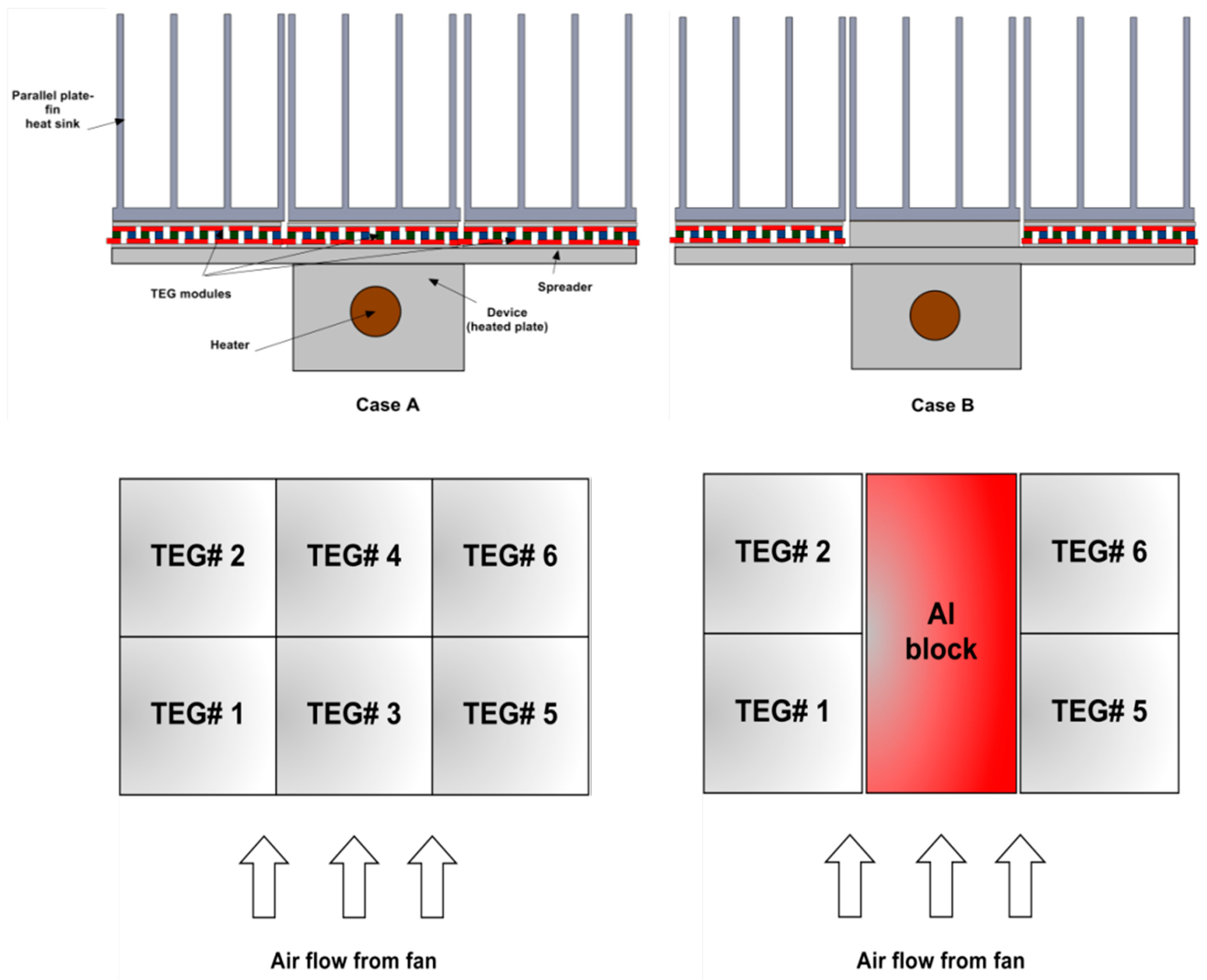
In this paper, the numerical models are used to simulate two types of physical models which are depicted in Figure 1 to explore potential better design for the self-power system that could be more efficient in operation. The first case is considered as a baseline model, which is designated as case A. It has six TEGs arranged between the heat sink and the heat source device. A heat spreader is placed between the heat source device and a number of TEGs organized in rectangular array. As depicted in the figure, these TEGs are labeled from TEG# 1 to TEG# 6. All the TEGs are placed on top of the spreader. For case A, two TEGs (TEG# 3 and TEG# 4) are placed in the middle while four TEGs, i.e., TEG# 1, TEG# 2, TEG# 5 and TEG# 6, are placed on the sides. TEG# 1, TEG# 3 and TEG# 5 are placed on the front side, with respect to the air flow that is pumped in from the fan, while the rest of the TEGs are placed on the back side. For case B model, TEG# 3 and TEG# 4 are replaced by an aluminum block of the same size occupied by the two TEGs. The rest of the TEGs have the same arrangement as case A. This arrangement enables the control of the temperature at higher heat flux input by reducing thermal resistance. The numerical results are compared and validated with experimental data based on the physical models. The application of the numerical methodology for the parametric study of heat sink geometry is also demonstrated.
2. Numerical Methodology
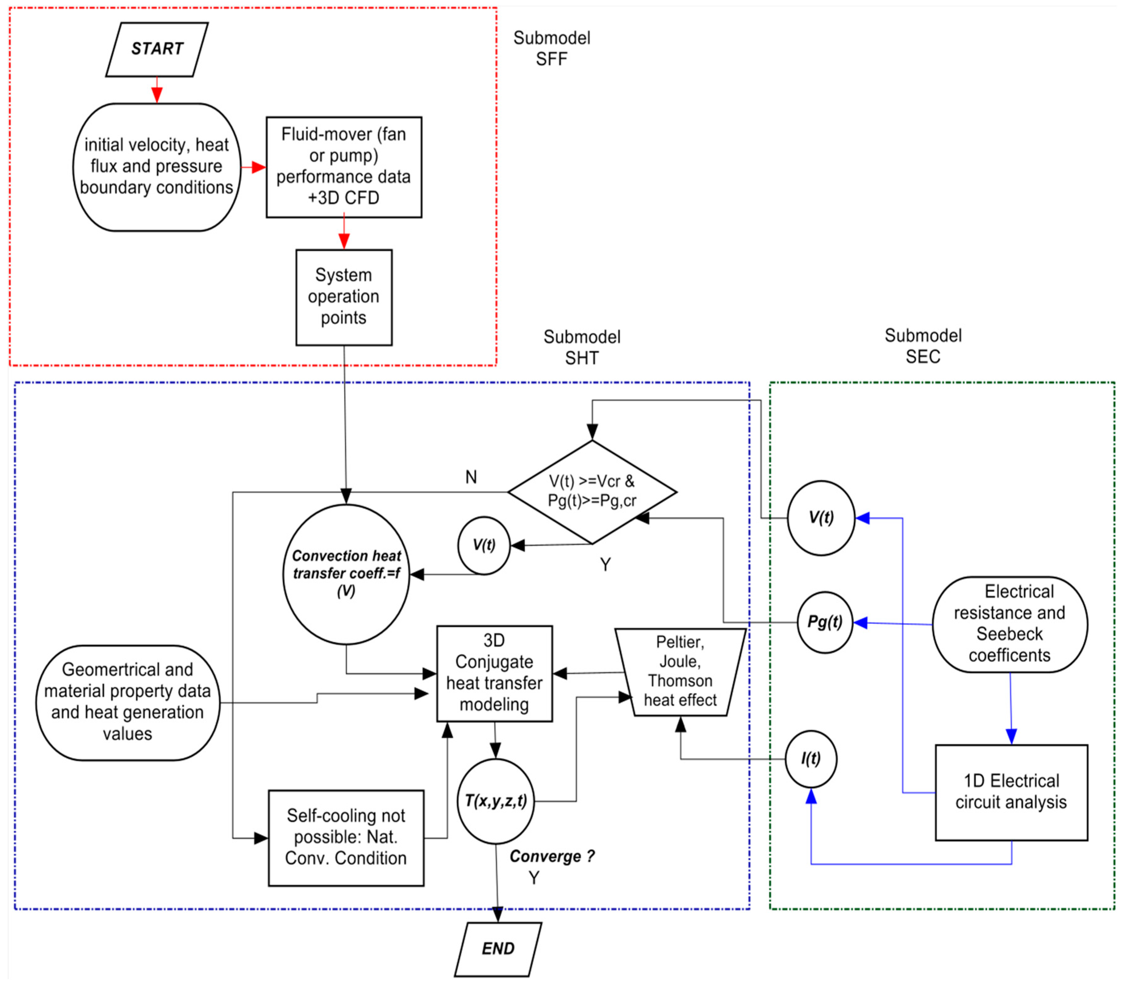
A general numerical methodology is developed which could be utilized to analyze TEG based self-cooling systems is shown in Figure 2. Details about the working principles in each blocks or submodels are explained in the following sections. In overall, for a given design configuration, the proposed methodology will start with the initial flow rate (or velocity) and pressure to determine the self-cooling system’s operation points. From there, the conjugate heat transfer in the device is solved with data exchange from the TEG’s electric circuit computation. The methodology is modularized, where fluid flow, heat transfer, and electric generation can be easily modeled and implemented for any complex design configurations or geometries. There are peculiar factors pertinent to the modeling of self-cooling system incorporating TEG modules. Firstly, the system has an internal loop in power generation. TEG modules provide the power for the fan/pump that cools the modules. Thus, an inlet condition for air flow into the cold side heat sink is coupled with the voltage and power generated from the modules. Secondly, TEG modules provide a variable voltage depending on temperature difference across the modules, thus, the fan/pump provides variable speed water/air flow (volume flow rate). Thirdly, as the TEG modules are placed between the heat source device and heat sink, there is a need for numerical modeling that helps to study the minimization of thermal resistance while providing enough temperature difference to power the cooling systems. There are three sub-models that constitute the general structure of the numerical methodology, which are a) submodel fluid flow (SFF), b) submodel conjugate heat transfer (SHT), and c) submodel electrical circuit (SEC).
Submodel fluid flow (SFF) represents three-dimensional fluid flow analyses in the fan (pump)-heat sink model. When pressure drop for self-cooling applications are considered, some important characteristics need to be considered. The operating points of the fan/pump should be defined at the intersection points between the fan/pump’s performance curves and the system resistance curves. It is well known that fan/pump manufacturers usually test and provide performance curves at only a rated voltage. However, what makes characteristic of self-cooling applications unique is that the voltage supplied to the fan/pump through TEGs is variable, and that could be quite different from rated voltage. Therefore, it is necessary to construct a performance curve of pressure drop vs volume flow rate for the fan/pump at different possible voltages.
In this study, the relationship between pressure drop versus volume flow rate at a rated voltage of 12 V has been extracted from the data sheet provided by the manufacturer [39]. We have used the well-known fan law relationships to construct the pressure drop versus volume flow rate curve at different voltage input values to the fan.
For a fixed impeller diameter (D), and if we assume pump/fan efficiency is constant within the frequency range, the following fan/pump affinity law are used to relate volume flow rate, , to the shaft speed, ω, at different voltages.
where xV and xV are the volume flow rate and shaft speed at a given voltage, respectively, while rV and rV are volume flow rate and shaft speed at the rated voltage, respectively.
Another affinity law that relates the pressure drop (head) at any given voltage (ΔpxV) to the pressure drop (head) at rated voltage (ΔprV) is by:
The ratio of fan /pump supply power at a certain voltage PxV to the power at rated voltage Prv relates in cubic power to the shaft speed is by the following affinity law:
The power is also related to the voltage Vx by the following equation:
where, the subscript “ld” indicated, Rld is the internal electrical resistance of the fan/pump.
Thus, ωxv is given by:
Equations (1) and (2) can be expressed in terms of input voltage by substituting the relationship from Equation (5).
Once the fan performance points at different voltage are derived using the relations mentioned above, the 3D fluid flow analysis is utilized to construct appropriate boundary conditions in two steps. In the first step, pressure drops at different flow rates for fan (pump)-heat sink model are simulated to construct the system operation curve. The operation curve is then super imposed on the fan/pump performance curve to identify system’s operation points which are found at the intersection points between the performance curves and system operation curve. It is thus possible to extract the volumetric flow relations as a function of input voltage to the fan (pump). In the second step, the volumetric flow conditions which represent the operation conditions of the system at variable voltages are then used as an input conditions to 3D fluid flow analysis to extract the average convection heat transfer coefficient (hav) for the particular fan (pump)-heat sink model. The values of hav as a function of input voltage to the fan (pump) are used as convection boundary conditions for the subsequent model. For an input voltage or power less than starting voltage (Vcr) or starting power (Pcr) of the fan (pump), natural convection conditions apply.
Submodel conjugate heat transfer (SHT) contains the components of the self-cooling device except the fluid domain. SHT has surface boundary conditions that are obtained from SFF. The heat generation rate of the device is also an input parameter to the model. In SHT, the governing equations of conservation of energy are applied to calculate the temperature distribution in the whole device setup. These include heat source device, heat spreaders, TEG modules and parts of the heat sink. There are also planar and volumetric heat generation rates inside the TEG module which are given by Peltier, Joule and Thomson heat effects. The heat generation values are functions of the current flow inside the TEG modules. Thus, it is also necessary to have submodel electrical circuit (SEC) which calculates the current, voltage and power from TEG modules. SEC basically contains 1D equations which relate current and voltage as a function of temperature difference across the TEG modules. Thus, we have a loop by which SHT supplies temperature values to SEC which in turn furnishes heating rates back to SHT. SEC also supplies the voltage value at each iteration and time step so that the appropriate boundary condition value is applied in SHT.
3. Numerical Model
The numerical computational strategy could be solved in any appropriate software or could be coded in a relevant programming language. However, the use of dedicated computational fluid CFD software with ability to integrate user defined functions ensures various complexities of heat sink and device set up could be readily handled in SFF and SHT. Although the modeling strategy can be implemented in either finite element model (FEM) or FVM models, in the following section of the paper, only the analysis using FVM model is presented.
User Defined Functions Based Modeling in FVM Model
In this section, an FVM-based commercial CFD software (ANSYS Fluent 14) [20] is used to implement the computational strategy. In Fluent, inbuilt CFD capabilities are integrated with UDF written in ANSI-C. Two computational domains namely domain A and B are constructed. Domain A represents SFF and domain B has both SHT and SEC integrated into the domain.
For a comparison with experimental data, domain A is used to identify the operational points of the fan-heat sink assembly for a given fan used in experiments. It supplies a surface boundary condition to domain B using an interpolating UDF. Domain A contains the air domain and the heat sink only. At the inlet, the volume flow rate of the fan is varied as an input condition. The outlet condition from the domain is zero gage pressure boundary conditions. The governing equations for three-dimensional, forced, unsteady state and incompressible fluid flow are solved. Domain B is comprised of the heat sink, extender, array of TEG modules, spreader, heat source heater and the plate.
Fully coupled multiphysics modeling technique is used to model fluid flow, heat transfer and electrical subsystems in domain A and B. The governing equations for the three-dimensional, forced, transient incompressible fluid flow and heat transfer in the heat source device, heat spreader, TEG, cold-side extender, dissipater and air subdomain are solved.
The general equations for continuity, momentum and energy or heat transfer for the device are given as follows.
Continuity equation:
where u, v and w are the fluid velocity components in x, y and z directions respectively.
Momentum equations in x, y and z coordinate:
where p is the pressure field.
Energy equation:
where, SQ is a source term due to the volumetric heat generation (, which is produced from the heater of the device.
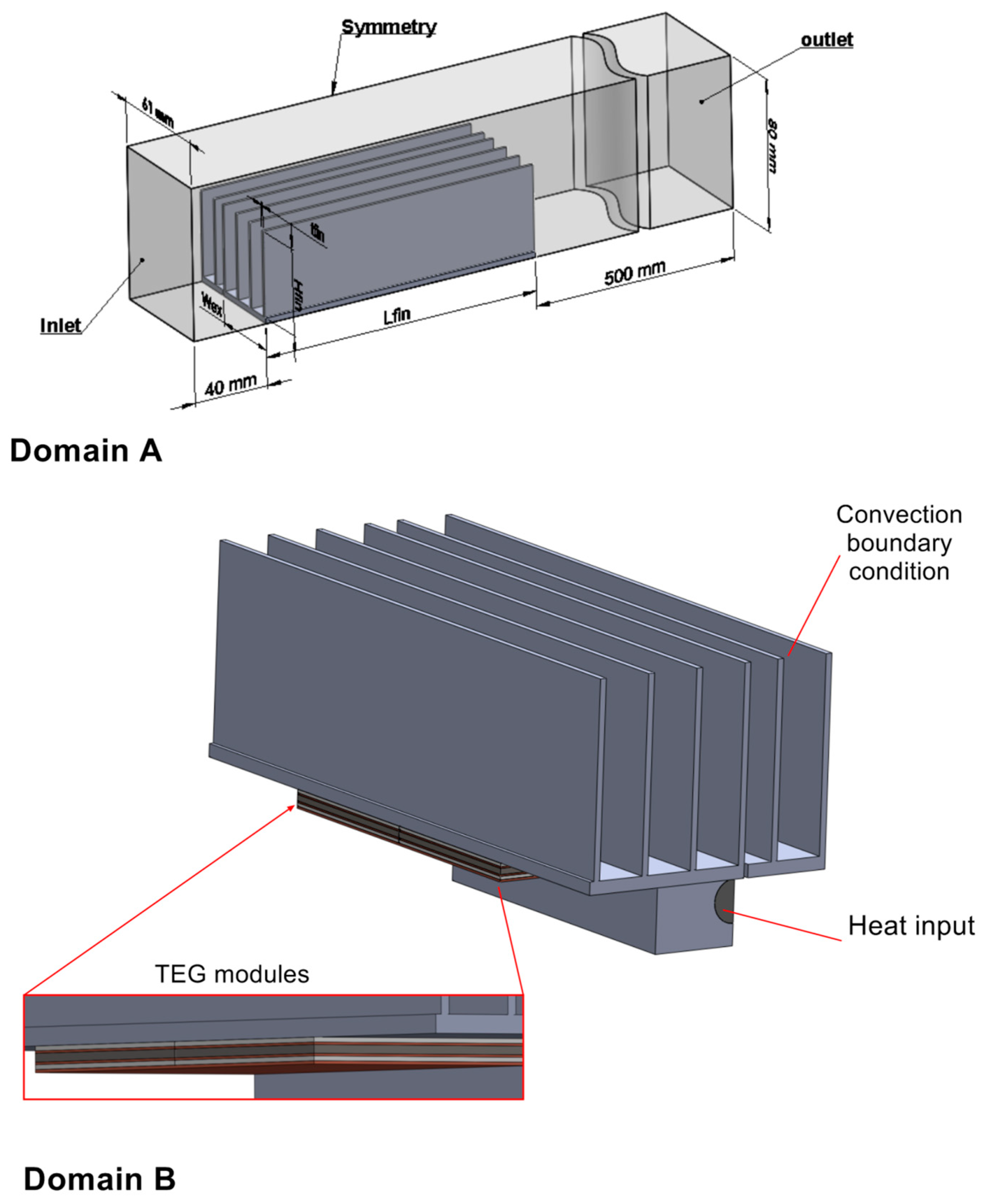
The computational domains and boundary condition are depicted in Figure 3. For the numerical simulation, a uniform volumetric heat generation ( is assumed in a heater. All surfaces of the heated plate except the side in contact with the spreader are assumed to be insulated. The ambient temperature is taken as 298 K. Adiabatic boundary conditions were applied to TEG walls exposed to the environment. This is primarily because during our experimental measurement, all the TEG walls were insulated by foam insulation materials.
Also, the thermal radiation heat transfer was not considered in the simulation in the present study. Due to the forced convection provided by the fan, radiation heat transfer from the fin surfaces was estimated to be negligible. As commented above, all TEG walls are insulated during the experiments.
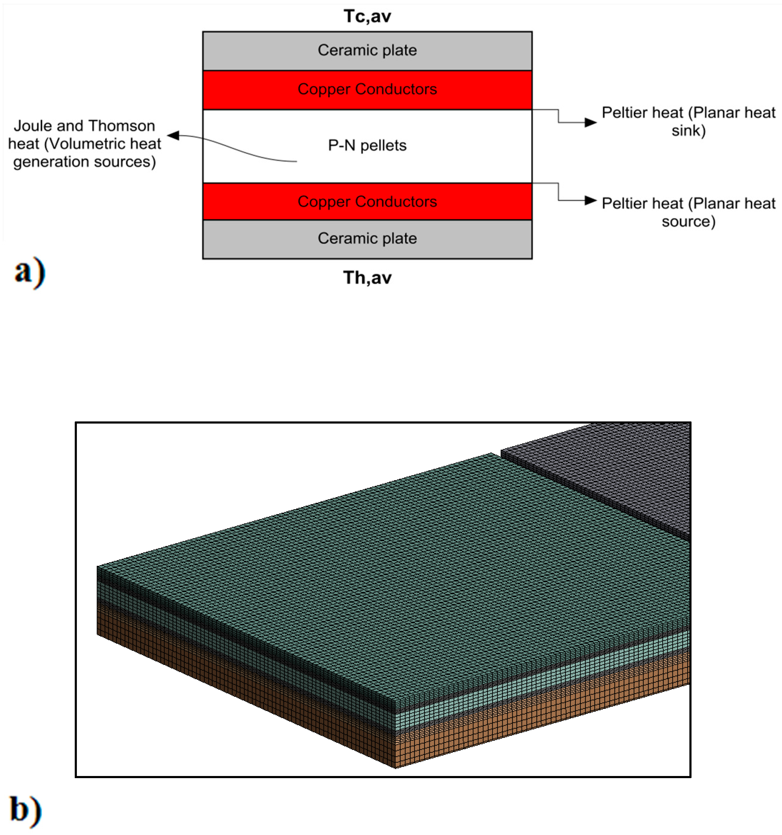
A thermoelectric module consists of number of TEG modules connected in series by copper solder and contained between thermally conductive and electrically insulated ceramic plates. The simulation of numerous P–N pairs inside each module in an array would result in high computational complexity in terms of grid size as well as computational time [40]. Thus, the TEG module is modeled as TEG cuboid consisting of three parts as shown in Figure 4. The first part represents the P and N semiconductor pellets with an air gap. It is modeled as a combined pellet-air gap cuboid by aggregating the properties of the P and N legs and the air gap in between using the weighted mean method. The air gap’s volume is proportional to the actual space between the P and N legs.
The thermal properties of aluminum, copper and ceramic materials used in the TEG device at an average temperature of 350 K is shown in Table 1 [41].
The thermal properties of the Seebeck coefficient, thermal conductivity and resistance for the P–N elements are assumed to isotropic, and can be calculated using the following formulas, which are from [42]. Readers can refer this reference for how they were developed.
The second part is the copper conductors on both sides of the pellet-air gap cuboid. The copper conductors are also aggregated into a homogenous conductor cuboid by similar method used for the semi-conductor pellets. The third part is the cold and hot side ceramic plates. At the interface between the cold-side ceramic plate and the base of the heat sink and hot side of ceramic plate and spreader, there exits an interfacial contact thermal resistance.
Thus, the thermal properties of the ceramic plates have been modified to account of the extra contact thermal resistance. The value for the contact thermal resistance has been estimated from experimental data. Its change with temperature was not considered.
For an array of TEG modules that are connected in series to a load, the total voltage at any given instant t, VT (t) and the current in the array, I(t) are given as:
where m is the number of modules in an array and Th,av_j(t) and Tc,av_j(t) are the average hot side and cold side temperature of the j-th TEG module at an instant t, respectively. Tm,av is the average temperature of the TEG module. Re,TEG, Re,ld, and Re,c are the electrical resistances of the TEG module, load, and circuit wire, respectively.
The = supply power of the fan/pump is also related to the fan supply voltage Vx by the equation:
For the m number of modules connected in series electrically in an array, the average temperature of hot side and cold side of the jth TEG module could be calculated as:
where [t0, t1] is a time interval, Ω is the spatial derivative for the j-th module. Th,av and Tc,av are calculated at the hot and cold surface of the TEG module, respectively.
Peltier heat at the interface of hot side of TEG and copper solder at a j-th module in an array of TEG modules is given as:
where ATEG,h is the hot side area of TEG module
Peltier heat at the interface of cold side of TEG and copper solder is given as:
where ATEG,c is the cold side area of TEG module.
The Joule and Thomson heat are modeled as volumetric heat generation in the P–N pellet region and could be written as:
where first and second term in the equation are the Joule and Thomson heat respectively, LPN is the height of the P-N pellet region and Rel,PN is the electrical resistivity of P and N thermoelectric pairs. Equations (20)–(22) used instantaneous values for the calculation. Due to neglecting the unsteady process-related terms, their forms look similar to the formula for steady process. However, as shown in later sections, experimental test results agree with the modelling, which confirmed that such treatment is acceptable for the present problem.
From the equation it could be seen that, the heat terms are a function of the current flowing inside the module and the current is again dependent on the temperature difference between the TEG module surfaces. Thus, it is important to employ a numerical methodology which iteratively calculates for the current and voltage inside the array. The capability of employing UDFs written in ANSI C programming language in ANSYS Fluent [20] is employed to include the electrical and heat terms. The entire computational procedure was tested and found repeatable. In the CFD simulation, grid independent study was performed to ensure the results are consistent for different configurations [14]. Second-order accurate numerical schemes were used, and the convergence criteria were set to be 10−6 of residuals for all the governing flow equations.
The above numerical model is applicable for any flow that is laminar or at low Reynolds numbers (ReDh < 2100). It can be used for any levels of voltage and input power within the permissions of the fan and TEG.
4. Experimental Data
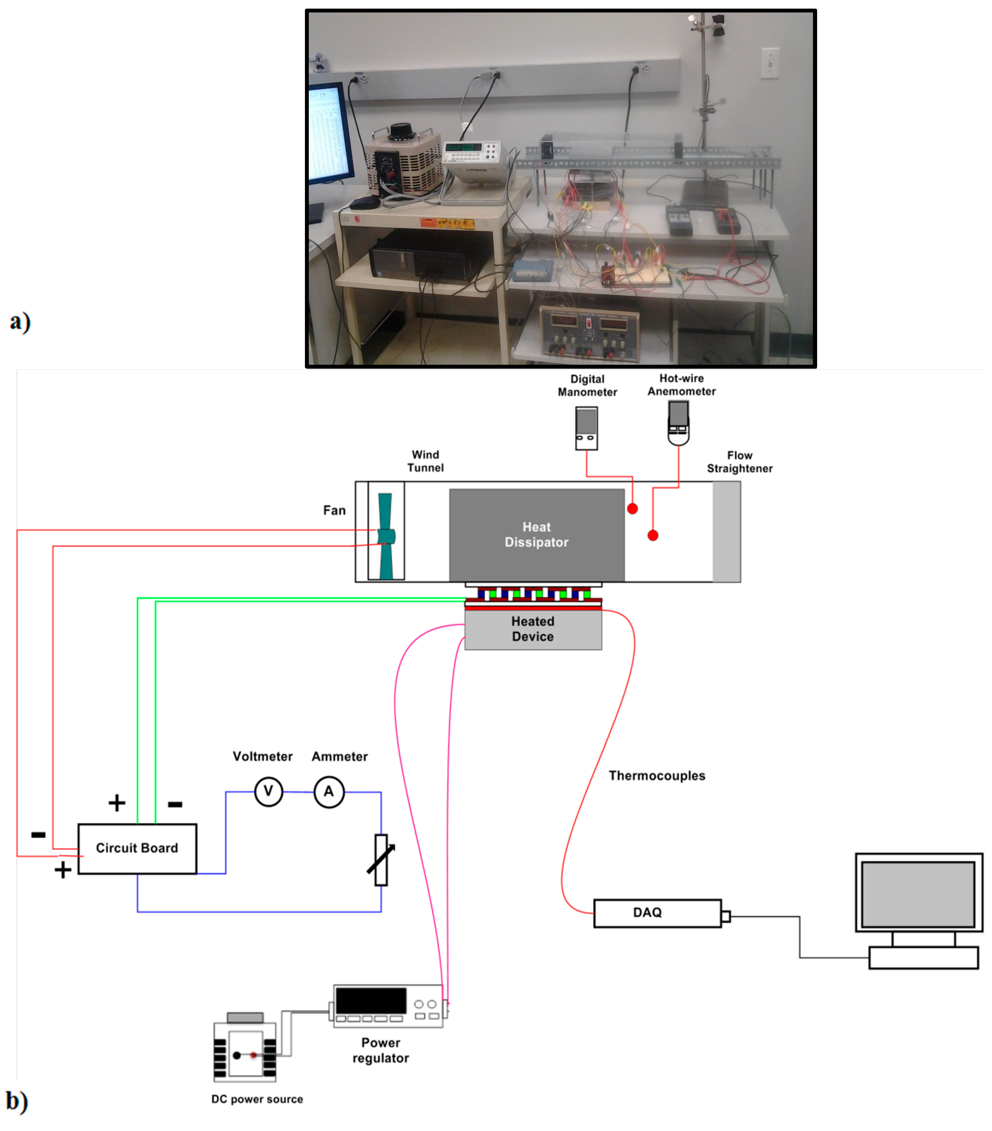
The schematic of the experimental setup is depicted in Figure 5. An aluminum plate of dimensions of 80 × 40 × 20 mm3 represents a heat source device. A cartridge heater (Omega CSH-303535) with 12.7 mm diameter and 76 mm in length was fitted inside the plate tightly to provide a uniform volumetric heating to the plate. It has a maximum heating capacity or 535 W (21 W/cm2) and a sheath temperature of 760 °C. An adjustable DC power provides heating power to the cartridge heater. We wrapped around all exposed surfaces of the heated plate using thermal insulation materials to prevent heat loss to the environment. At the maximum heat power, the external temperature of the insulating materials surrounding the device was found to be almost at the temperature as the ambient air, i.e., heat loss was negligible. A precise control of heating power is provided using a digital meter/power regulator of Model GPM-8212 from GW Instek.
The heat spreader is made of aluminum, and has a 3.8 mm thickness and mm2 area to conduct heat from the device to an array of TEG modules (EVERREDTRONICS TEG241-1.0-1.2 model) which are inserted between the spreader and cold side heat sink. The heat sink and TEG were hold together by clamping devices with proper forces based on pre-test estimates to ensure best interface contact without mechanical deformation. The detailed TEG specification from the manufactures data is given in Table 2. Three separate heat sinks with finned parallel plate dissipater geometry are placed on the cold side of the TEG modules. Each of these dissipaters has a base area of 150 40 mm2, with 4 fins. The fin height is of 20 mm and the fin thickness is of 1.5 mm. The fin base is about 2 mm in thickness.
A high temperature thermal conductivity paste (OMEGATHERM) was placed in between all contacting surfaces in order to decrease contact resistance. A small wind tunnel, which was made of plexiglass was built to direct air flow over the dissipater. It had a cross-sectional area of 100 100 mm2 and a depth of 500 mm depth. A cooling fan (model SUNON EE92251S1) with dimensions of 92 92 25 mm was installed inside the wind tunnel, at 100 mm upstream of the dissipater. The velocity and temperature of the air flow at the wind tunnel outlet was measured by a hot wire anemometer/thermometer (model Control Company 4330). The volume flow rate was calculated based on the cross-sectional area of the wind.
Tunnel and the average flow velocity, which was obtained by measurements at multiple points and area-weighted averaging method. A digital manometer (OMEGA) is used to monitor the pressure drop in the heat sink. A data acquisition module (model USB 1008G from MC Computing) was used to log the temperature data collected from the glass-braided insulated thermocouples (OMEGA Engineering). The data logger was connected to a computer for data storage and analysis. An electrical circuit breadboard (model JE25 from JAMECO) was used as the platform for the TEG modules to be connected in series electrically. Voltage and current from the TEG modules is measured using a digital multimeter from WAVETEK (30XL model). All tests were repeated at least for three times to insure the accuracy of the test data.
The precisions of instruments are as follows:
GW Insel GPM-8213 power meter: voltage (±0.15%), current (±1%), power (±1%)
Omega K-type thermocouples: temperature (±1%)
Control Company hotwire anemometer: velocity (± 1%), temperature (± 0.8%)
5. Results and Discussion
5.1. Validation of the Numerical Model
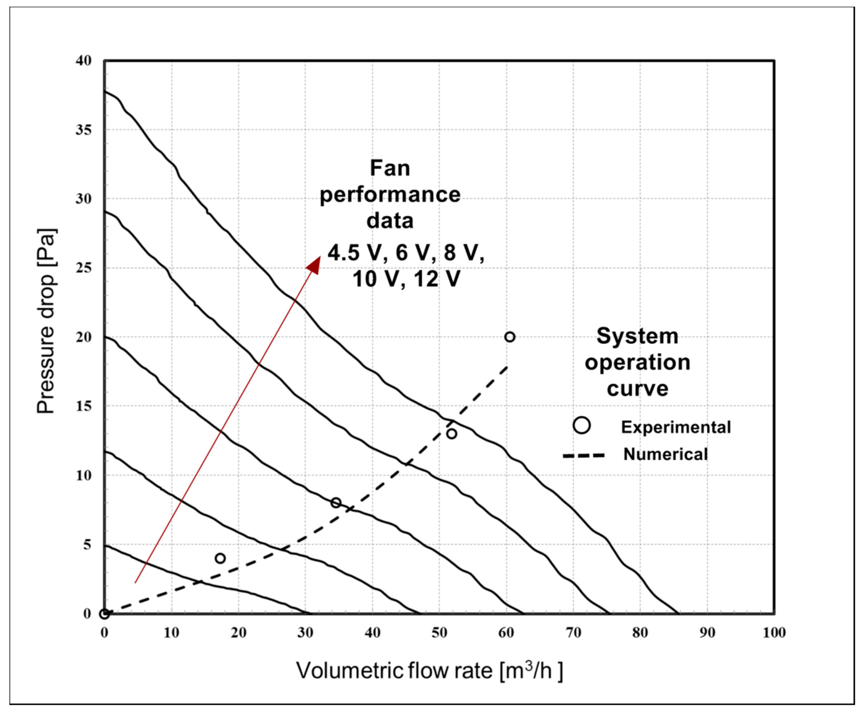
Figure 6 shows the fan performance data at varying voltages. The system operation curve for the heat sink geometry used in the experiment is superimposed on the fan performance data. The numerically simulated data is denoted by a full line while the experimental data is represented by dots. The system operation derived from CFD analysis has good agreement with experimental data. The intersection between the fan performance data at a given voltage and system operation curve indicates the operation point of the fan at that voltage. Therefore, the graph is useful to simulate heat sink pressure drop for different geometries and analyze how the system operates from the lowest starting voltage to the high rated voltage of the fan.
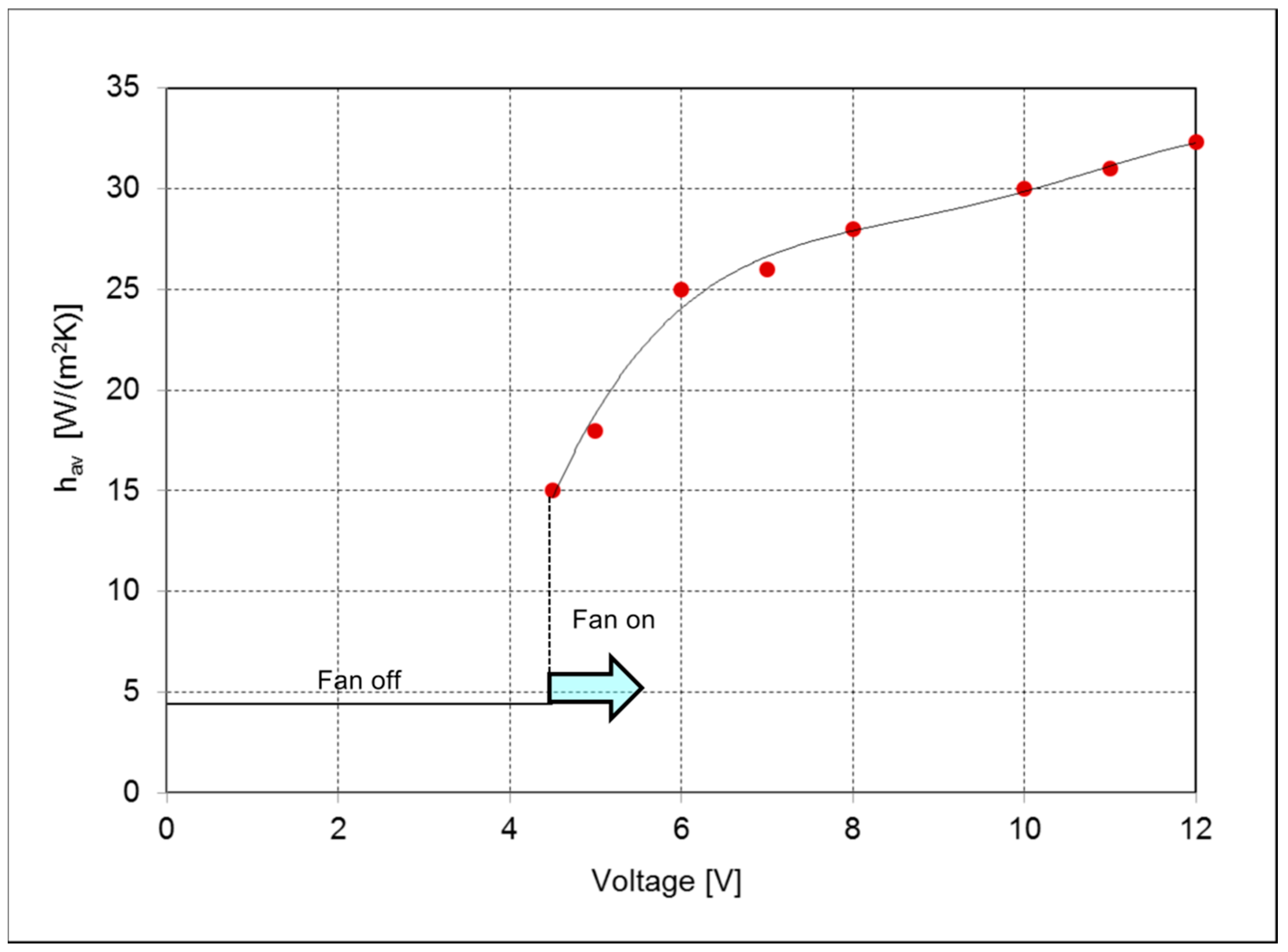
Figure 7 illustrates the relationship between average heat transfer coefficient and voltage input to the fan for the fan-heat sink model in Case A and B. The hav is computed by the FVM. It is the ratio of heat flux to the temperature difference between the heat sink’s base wall and air flow. It is evident that for the voltage less than Vcr, the fan does not rotate, therefore cooling off the device is via natural convection. Once the fan starts rotating, forced convection is the dominant means of heat dissipation from heat sink surfaces.
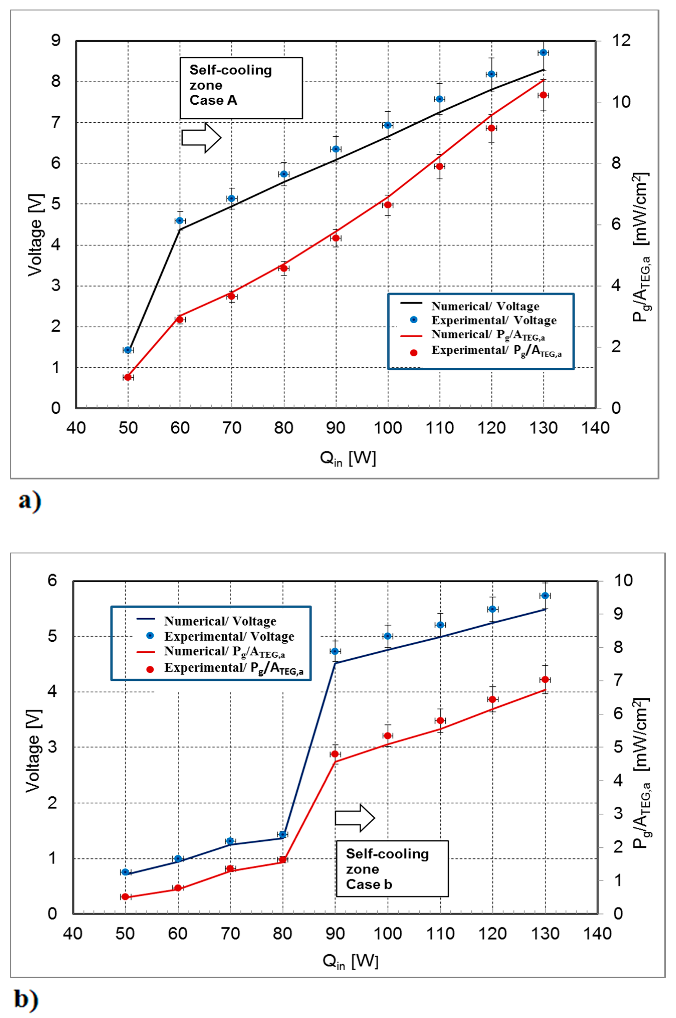
Figure 8a,b indicate open circuit voltage and power generated by TEG modules per area of TEG arrays as a function of heat input into a device for case A and B, respectively. The circular points indicate the experimental data while the lines show the simulated result. It could be observed that for the predicted results are in good agreement with experimental data (within 5%). The results show that self-cooling starts when the heat input into the device is at least 60 W and 90 W for case A and B, respectively.
At the self-cooling zone, the voltage produced by TEG arrays is at least equal to the starting voltage of the fan used in the experiment (Vcr = 4.5 V). when the fan starts to rotate, the internal resistance of the fan suddenly increases from 20 Ω to about 72 Ω.
This is marked by the jump in the fan supply voltage and power. Case A produces more total array voltage (38%) and power per area of TEG array (34%) than case B. This is due to the presence of more TEGs in the array and the position of pair of TEGs in direct heat path in case A.
Figure 9a,b show the transient simulation and experimental data of voltage produced by array of modules (VT) and temperature difference between the device and environment (ΔTde) for Qin = 120 W in Case B, respectively. The numerical simulation has been able to accurately predict both voltage and temperature difference within 5 % error margin. In the experiments, the fan starts to turn at 5 min after the heat input is applied at which instant the voltage reaches a value equivalent to Vcr as has been precisely simulated.
After the onset of the forced convection from the fan, the rate of change of temperature starts to decrease and the system achieves a steady state after 20 minutes. The temperature doesn’t show any appreciable change and the self-cooling has been able to control the temperature effectively.
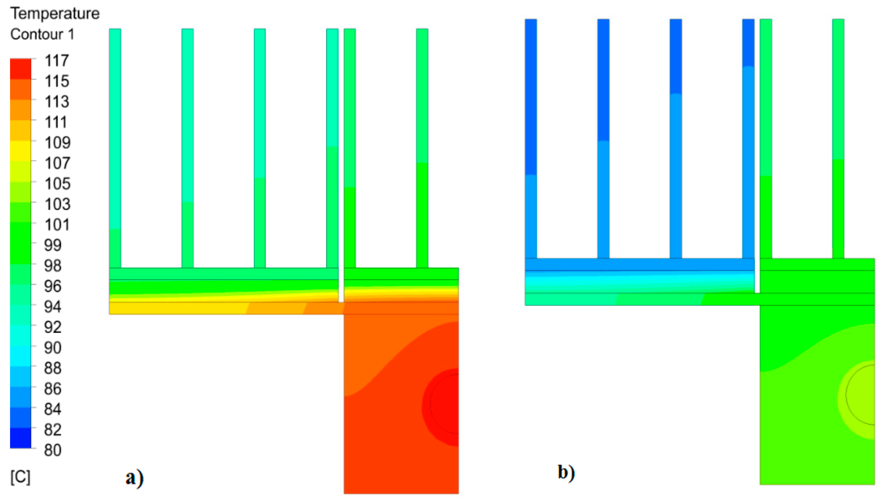
Figure 10 shows the typical transient simulation of temperature field in the entire TEG-heat sink system (only half domain is shown). The temperature contours are for Q = 130 W for case A and case B, respectively. Case B shows clearly that it can reach much lower temperature in the system.
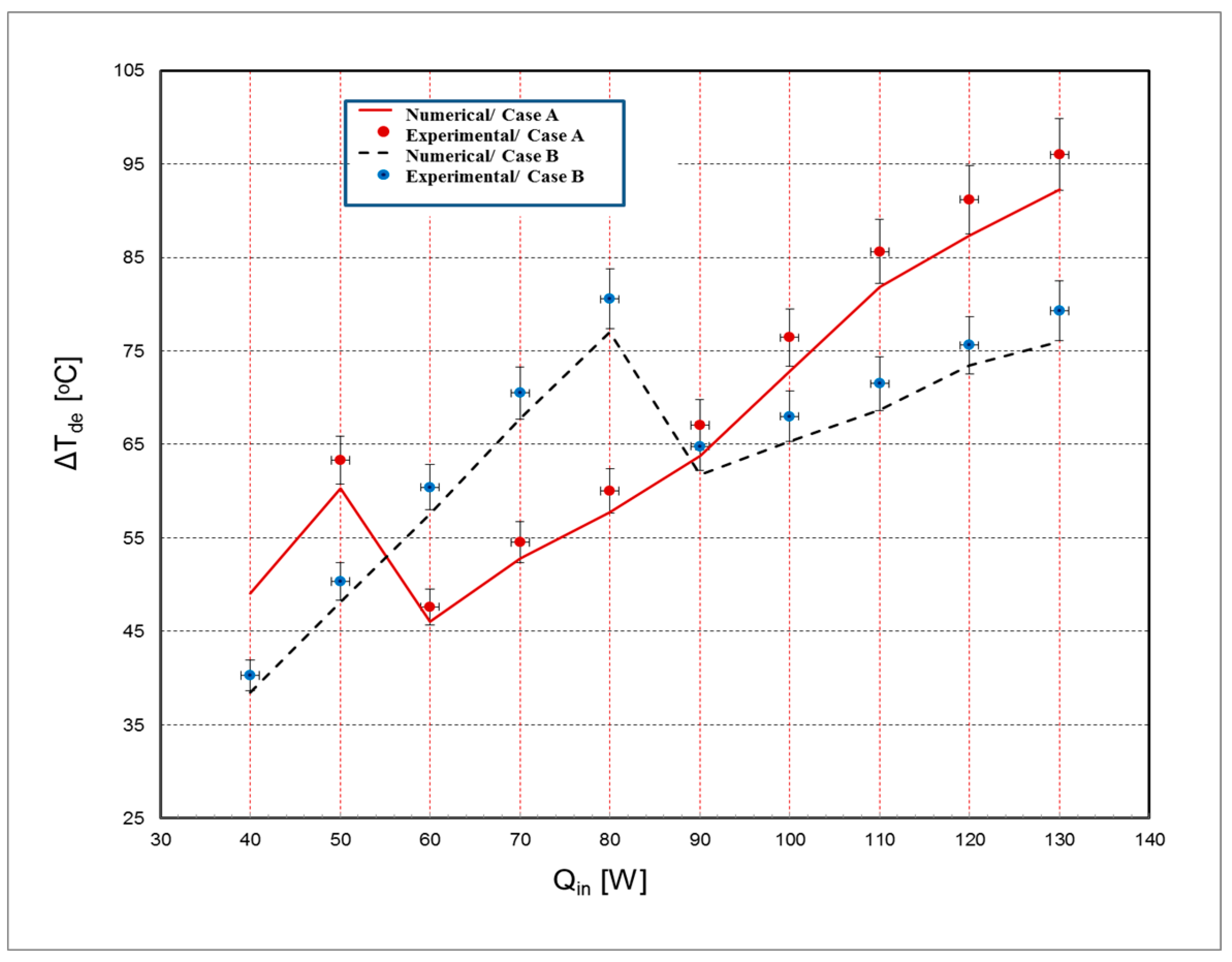
Figure 11. presents the variation of ΔTde (difference between temperature of device and environment) as a function of heat input into the device for case A and B. The numerical result has been able to predict the experimental data to good accuracy (within 5%). A sharp drop in temperature is observed at Qin = 60 W and 90 W for case A and B, respectively, due to the onset of self-cooling. In general, although case B produces less total array voltage and power per area of TEG, the temperature of the device has been able to be reduced as compared to case A. This is due to the presence of higher resistance in direct heat path in case A. The numerical result has been able to capture the phenomenon accurately.
5.2. Parametric Study using FVM Model
In the following section, the FVM model is used for parametric study of the effects of load resistance, fin height and fin density. It is well known that there are many other parameters that could affect the performance of the self-cooling system. Due to limited space, we limited our focus of the present paper on the investigating the effects of three parameters only, i.e., load resistance, fin height, and fin density.
5.2.1. Effect of Load Resistance
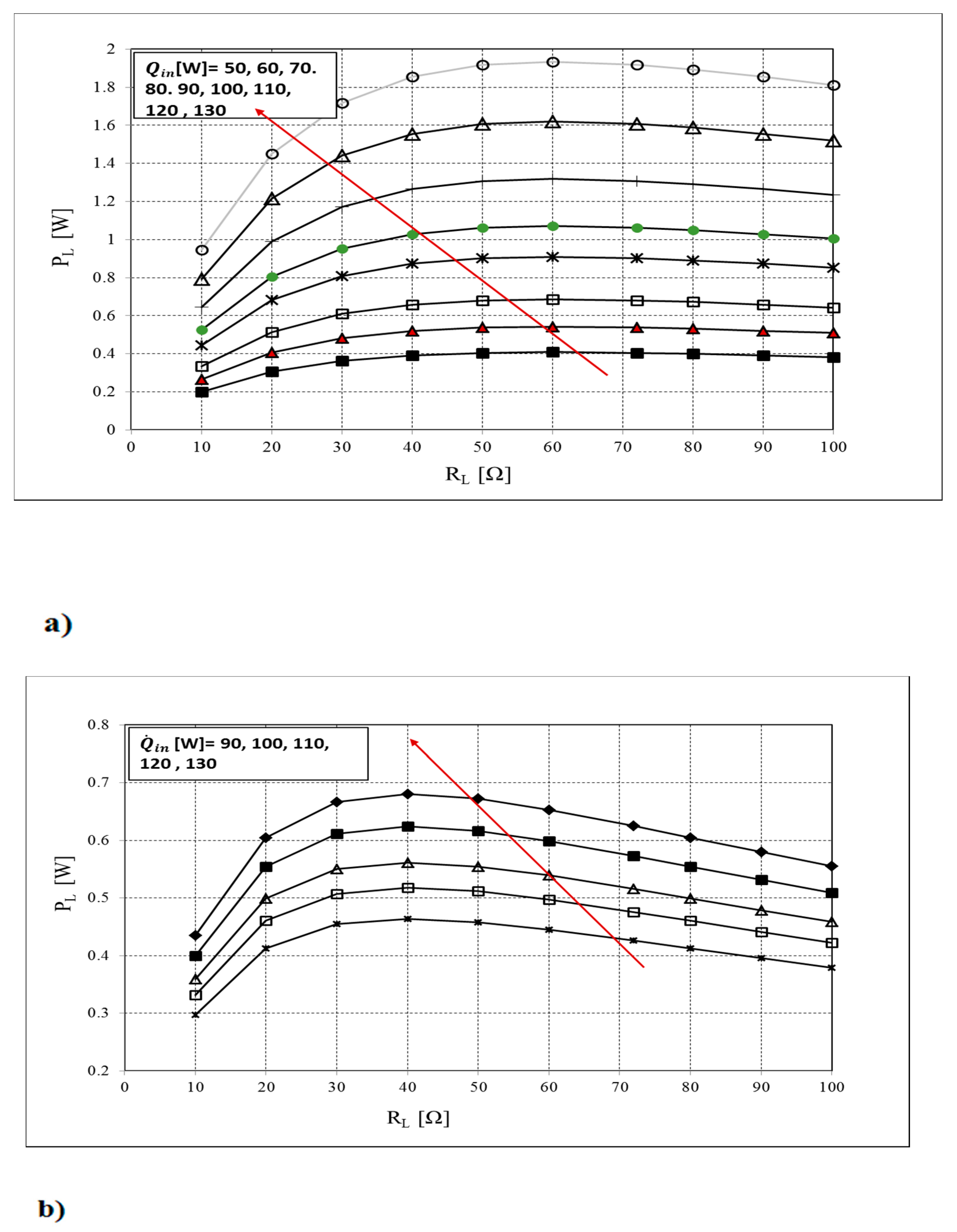
The electrical resistance of the fan (RL) affects the amount of power consumed by the fan. The effect of RL on PL for case A and B is shown in Figure 12. Each TEG module used in the experiments and simulation has an internal electrical resistance (RTEG) of 10 Ω. Thus, for case A, the system has maximum PL at when RL is equal to 60 Ω which is equivalent to the combined electrical resistance of the six TEGs connected in series. This is due to matched load condition which produces maximum power [24]. It can be inferred that PL could decrease by as much as 50% when a fan with 10 Ω is used for heat input of 130 W compared to the maximum point of operation. The fan used in the experiment has an internal resistance of 72 Ω producing a power close to the maximum possible power. For case B, the four TEGs have a cumulative RTEG of 40 Ω. Thus, the system produces 10 % less power when connected to the same fan as Case A. It is therefore important to match the electrical resistance of TEG arrays with the fan used in self-cooling applications.
5.2.2. Effect of Fin Height
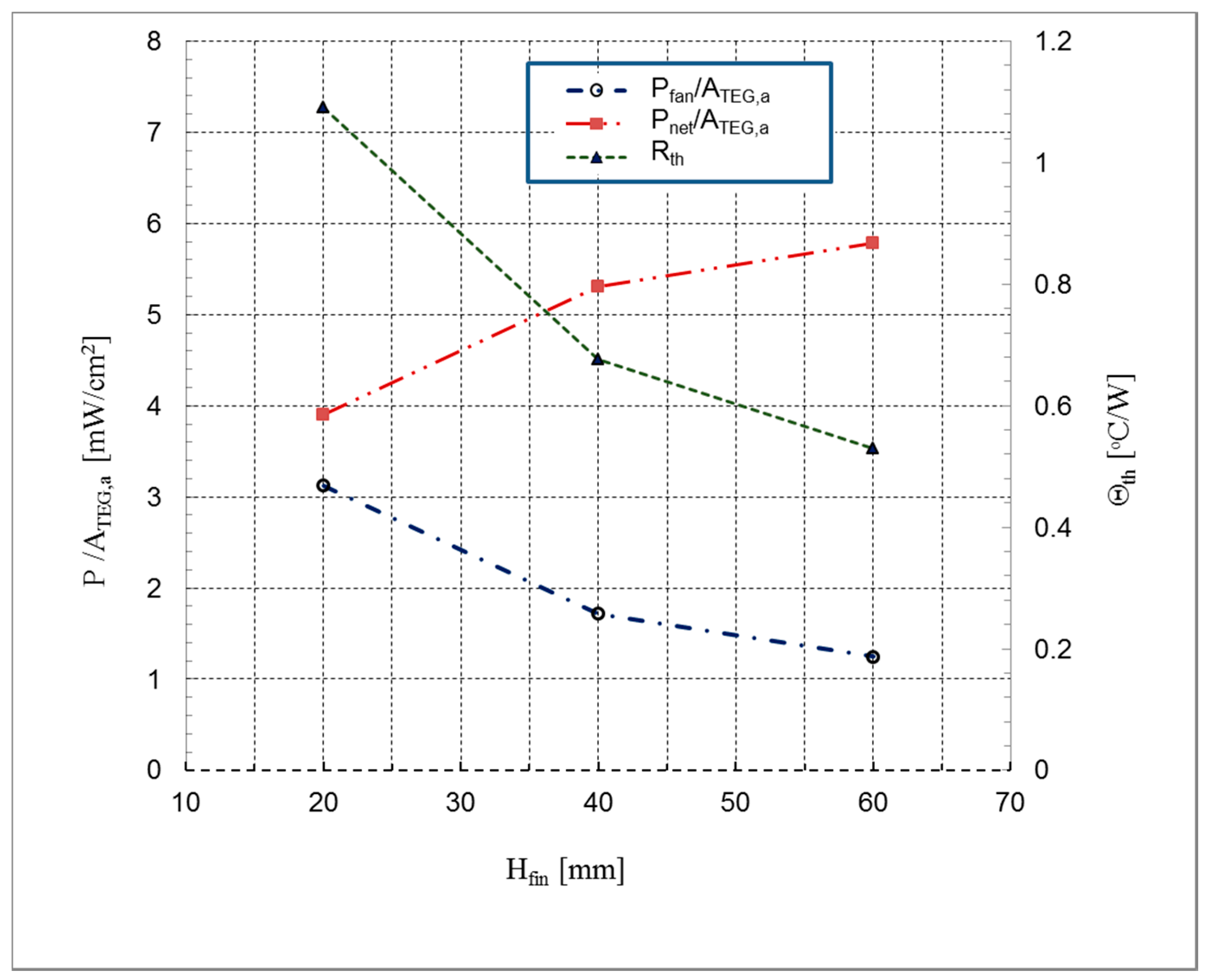
Figure 13 illustrates the numerical study of the variations of power supplied to the fan per area of TEG array (Pfan/ATEG,a), net power generated by TEG array (Pnet/ATEG,a) and overall device to environment thermal resistance (Θth,T) as a function of height of the fin (Hfin) in the heat sink. As the fin height is increased from 20 to 60 mm, the total area of the heat sinks is enlarged by about 167%. Thus, the thermal resistance is decreased by almost 50 % due to the availability of more area for heat transfer. In addition, the pumping power decreases slightly due to decreased friction losses. The velocity of the air in the channel is decreased, resulting in lower losses at higher fin heights. Thus, the net power generated by TEG module has also slightly risen.
5.2.3. Effect of Fin Density
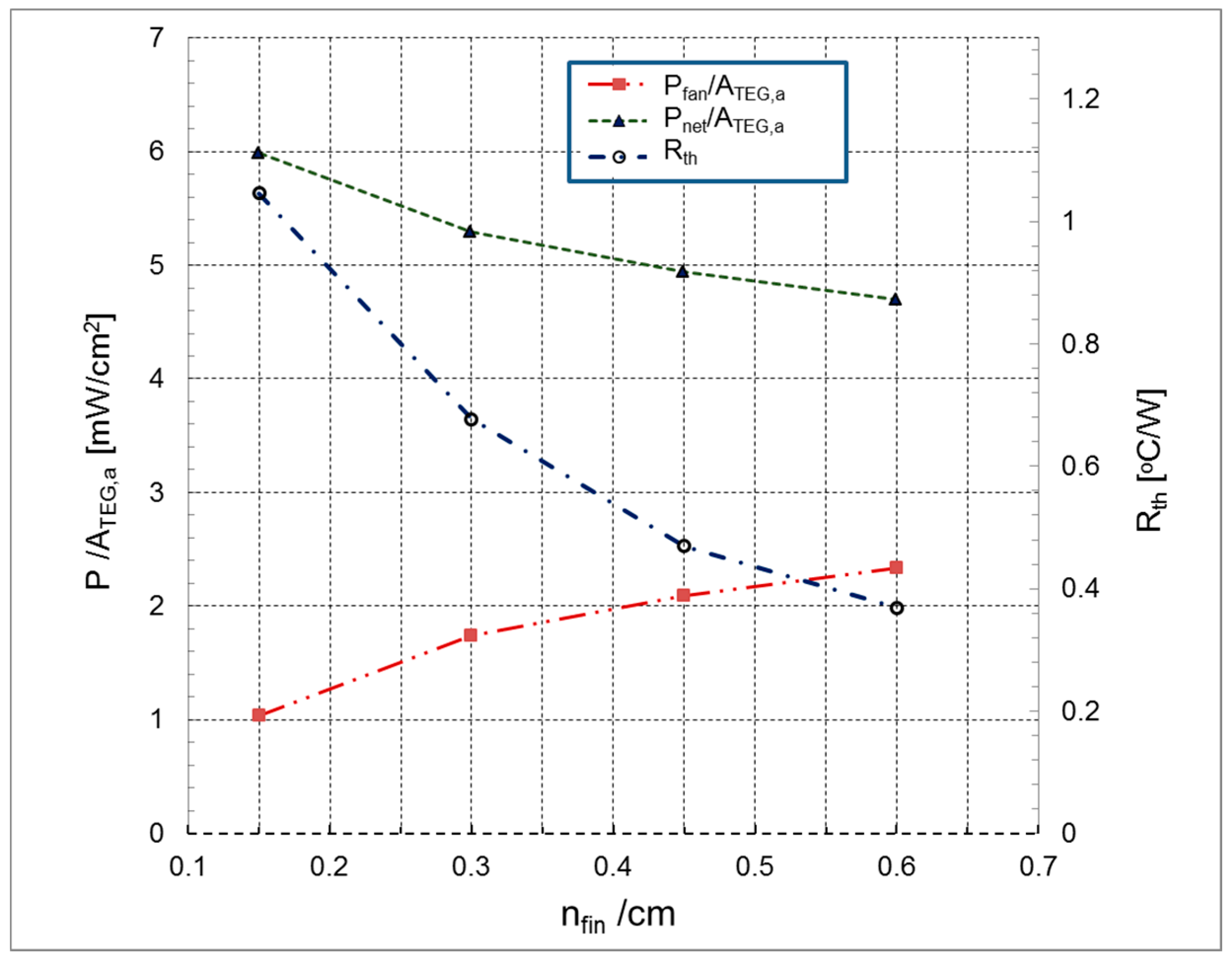
Figure 14 shows the numerical study of the effect of fin density (nfin) on values of pumping power, net power and thermal resistance. As the fin density is increased from 0.15 to 0.6, the total area of dissipaters increases by around 240%, thereby decreasing the total thermal resistance by 70%. However, as the fin density increases, the pressure drops in the dissipater rises requiring more power to be supplied to the fan. As a result, the net power produced by TEG array also declines as shown in the figure.
However, the system would still be able to provide self-cooling as long as a positive value of Pnet is achieved. Thus, the numerical simulation indicates that a more effective dissipater design in terms of increased surface area would make self-cooling more applicable for range of heat inputs.
6. Conclusions
In this study, a general methodology for the study of TEG-based self-cooling is developed. The methodology has three major parts. The fluid flow domain which is used to the study the effect of a variable speed fan and on the heat transfers and derive a relation of convection heat transfer coefficient with input voltage. The temperature and electric field variation is then studied using a coupled approach using an input from the fluid domain as boundary condition. Experiments have been conducted on two types of self-cooling arrangements to measure the device temperature, voltage, and power produced by TEG modules. It has been shown that the numerical model developed in this research is able to predict the data from instrumented experiments with good accuracy, within an error of less than 5%. A parametric study on the effect of electrical resistance of load (RL), height of fin (Hfin) and fin density (nfin) has been made. It was found that the power for self-cooling could be maximized by proper matching of number of TEG modules to the fluid mover (fan or pump) in terms of electrical resistance. An increase in Hfin decreases the fan power consumption and thermal resistance. It has also been shown that although an increase in nfin results in rise in fan power consumption, there is a marked increase in net power and decreases in thermal resistance.
Author Contributions
Writing—original draft preparation, R.K.; writing—review and editing, C.-X.L.
Funding
This research received no external funding.
Conflicts of Interest
The authors declare no conflict of interest.
Nomenclature
| A | area (m2) | volume flow rate (m3/s) | |
| Cp | specific heat (J/kg K) | ||
| h | heat transfer coefficient (W/m2 K) | Greek symbols | |
| I | electric current ( A) | α | seebeck coefficient (V/K) |
| L | length (m) | ρf | fluid density (kg/m3) |
| m | number of modules in an array | τ | Thermal diffusivity (m2/s) |
| Np | number of semiconductor pairs | ||
| P | electrical power (W) | Subscripts | |
| Δp | pressure drop (Pa) | cer | ceramic |
| heat flux (W/m2) | cu | copper | |
| heat input to device (W) | fb | fin base | |
| T | temperature (°C) | fin | parallel-plate fins |
| fluid velocity (m/s) | h | hot side | |
| μf | dynamic viscosity (N.s/m2) | mod | module |
| Rel | electrical resistance (Ω) | P-N | P and N semiconductor pairs |
| Rth | thermal resistance (°C/W) | p | P elements in TEG module |
| S | source term of energy equation | n | N elements in TEG module |
| V | voltage (V) | s | spreader |
References
- Date, A.; Date, A.; Dixon, C.; Akbarzadeh, A. Progress of thermoelectric power generation systems: Prospect for small to medium scale power generation. Renew. Sustain. Energy Rev. 2014, 33, 371–381. [Google Scholar] [CrossRef]
- Gou, X.; Xiao, H.; Yang, S. Modeling, experimental study and optimization on low-temperature waste heat thermoelectric generator system. Appl. Energy 2010, 87, 3131–3136. [Google Scholar] [CrossRef]
- Liu, X.; Li, C.; Deng, Y.; Su, C. An energy-harvesting system using thermoelectric power generation for automotive application. Int. J. Electr. Power Energy Syst. 2015, 67, 510–516. [Google Scholar] [CrossRef]
- Khattab, N.M.; El Shenawy, E. Optimal operation of thermoelectric cooler driven by solar thermoelectric generator. Energy Convers. Manag. 2006, 47, 407–426. [Google Scholar] [CrossRef]
- Zhu, N.; Matsuura, T.; Suzuki, R.; Tsuchiya, T. Development of a Small Solar Power Generation System based on Thermoelectric Generator. Energy Procedia 2014, 52, 651–658. [Google Scholar] [CrossRef] [Green Version]
- Shi, Y.; Wang, Y.; Deng, Y.; Gao, H.; Lin, Z.; Zhu, W.; Ye, H. A novel self-powered wireless temperature sensor based on thermoelectric generators. Energy Convers. Manag. 2014, 80, 110–116. [Google Scholar] [CrossRef]
- Champier, D.; Bédécarrats, J.; Kousksou, T.; Rivaletto, M.; Strub, F.; Pignolet, P. Study of a TE (thermoelectric) generator incorporated in a multifunction wood stove. Energy 2011, 36, 1518–1526. [Google Scholar] [CrossRef] [Green Version]
- Liu, X.; Deng, Y.; Zhang, K.; Xu, M.; Xu, Y.; Su, C. Experiments and simulations on heat exchangers in thermoelectric generator for automotive application. Appl. Therm. Eng. 2014, 71, 364–370. [Google Scholar] [CrossRef]
- Deng, Y.; Zhu, W.; Wang, Y.; Shi, Y. Enhanced performance of solar-driven photovoltaic–thermoelectric hybrid system in an integrated design. Sol. Energy 2013, 88, 182–191. [Google Scholar] [CrossRef]
- He, W.; Su, Y.; Wang, Y.; Riffat, S.; Ji, J. A study on incorporation of thermoelectric modules with evacuated-tube heat-pipe solar collectors. Renew. Energy 2012, 37, 142–149. [Google Scholar] [CrossRef]
- Kim, K.J.; Cottone, F.; Goyal, S.; Punch, J. Energy scavenging for energy efficiency in networks and applications. Bell Labs Tech. J. 2010, 15, 7–29. [Google Scholar]
- Kiflemariam, R.; Lin, C.-X. Numerical simulation of integrated liquid cooling and thermoelectric generation for self-cooling of electronic devices. Int. J. Therm. Sci. 2015, 94, 193–203. [Google Scholar] [CrossRef]
- Kiflemariam, R.; Lin, C.-X.; Moosavi, R. Numerical simulation, parametric study and optimization of thermoelectric generators for self-cooling of devices. In Proceedings of the 11th AIAA/ASME Joint Thermophysics and Heat Transfer Conference, Atlanta, GA, USA, 16–20 June 2014. [Google Scholar]
- Kiflemariam, R.; Lin, C.-X. Numerical Simulation and Parametric Study of Heat-Driven Self-Cooling of Electronic Devices. J. Therm. Sci. Eng. Appl. 2015, 7, 011008. [Google Scholar] [CrossRef]
- Martínez, A.; Astrain, D.; Rodríguez, A. Experimental and analytical study on thermoelectric self cooling of devices. Energy 2011, 36, 5250–5260. [Google Scholar] [CrossRef]
- Yazawa, K.; Solbrekken, G.; Bar-Cohen, A. Thermoelectric-powered convective cooling of microprocessors. IEEE Trans. Adv. Packag. 2005, 28, 231–239. [Google Scholar] [CrossRef]
- Solbrekken, G.; Yazawa, K.; Bar-Cohen, A. Heat driven cooling of portable electronics using thermoelectric technology. IEEE Trans. Adv. Packag. 2008, 31, 429–437. [Google Scholar] [CrossRef]
- Gould, C.; Shammas, N.; Grainger, S.; Taylor, I. Thermoelectric cooling of microelectronic circuits and waste heat electrical power generation in a desktop personal computer. Mater. Sci. Eng. B 2011, 176, 316–325. [Google Scholar] [CrossRef]
- Martinez, A.; Astrain, D.; Rodriguez, A. Dynamic model for simulation of thermoelectric self cooling applications. Energy 2013, 55, 1114–1126. [Google Scholar] [CrossRef]
- Ansys Inc. Ansys Fluent Theory and User Guide, Release 14; Ganonsburg: Pennsylvania, PA, USA, 2011. [Google Scholar]
- Chen, L.; Gong, J.; Sun, F.; Wu, C. Effect of heat transfer on the performance of thermoelectric generators. Int. J. Therm. Sci. 2002, 41, 95–99. [Google Scholar] [CrossRef]
- Zebarjadi, M. Heat Management in Thermoelectric Power Generators. Sci. Rep. 2016, 6, 20951. [Google Scholar] [CrossRef] [Green Version]
- Shukla, K.N. Thermal math modeling and analysis of an electronic assembly. J. Electron. Packag. 2001, 123, 372–378. [Google Scholar] [CrossRef]
- Jónsson, H.; Moshfegh, B. Modeling of the thermal and hydraulic performance of plate fin, strip fin, and pin fin heat sinks-influence of flow bypass. IEEE Trans. Compon. Packag. Technol. 2001, 24, 142–149. [Google Scholar] [CrossRef]
- Saini, M.; Webb, R.L. Heat rejection limits of air cooled plane fin heat sinks for computer cooling. InITherm 2002. In Proceedings of the Eighth Intersociety Conference on Thermal and Thermomechanical Phenomena in Electronic Systems (Cat. No. 02CH37258), San Diego, CA, USA, 30 May–1 June 2002. [Google Scholar] [CrossRef]
- Shukla, K. Hydrodynamics of diffusive processes. Appl. Mech. Rev. 2001, 54, 391–404. [Google Scholar] [CrossRef]
- Ko, T.; Ting, K. Optimal Reynolds number for the fully developed laminar forced convection in a helical coiled tube. Energy 2006, 31, 2142–2152. [Google Scholar] [CrossRef]
- Hajmohammadi, M.R.; Lorenzini, G.; Shariatzadeh, O.J.; Biserni, C. Evolution in the Design of V-Shaped Highly Conductive Pathways Embedded in a Heat-Generating Piece. J. Heat Transf. 2015, 137, 061001. [Google Scholar] [CrossRef]
- Hajmohammadi, M.R.; Moulod, M.; Joneydi Shariatzadeh, O.; Nourazar, S.S. Essential reformulations for optimization of highly conductive inserts embedded into a rectangular chip exposed to a uniform heat flux. J. Mech. Eng. Sci. 2014, 228, 2337–2346. [Google Scholar] [CrossRef]
- Hajmohammadi, M.R.; Maleki, H.; Lorenzini, G.; Nourazar, S.S. Effects of Cu and Ag nano-particles on flow and heat transfer from permeable surfaces. Adv. Powder Technol. 2014, 26, 193–199. [Google Scholar] [CrossRef]
- Hajmohammadi, M.R.; Pouzesh, A.; Poozesh, S. Controlling the heat flux distribution by changing the thickness of heated wall. J. Basic Appl. Sci. 2012, 2, 7270–7275. [Google Scholar]
- Hajmohammadi, M.; Nourazar, S.; Campo, A.; Poozesh, S. Optimal discrete distribution of heat flux elements for in-tube laminar forced convection. Int. J. Heat Fluid Flow 2013, 40, 89–96. [Google Scholar] [CrossRef]
- Najafi, H.; Najafi, B.; Hoseinpoori, P. Energy and cost optimization of a plate and fin heat exchanger using genetic algorithm. Appl. Therm. Eng. 2011, 31, 1839–1847. [Google Scholar] [CrossRef]
- Memon, S.; Tahir, K.N. Experimental and analytical simulation analyses on the electrical performance of thermoelectric generator modules for direct and concentrated Quartz-Halogen heat varvesting. Energies 2018, 11, 3315. [Google Scholar] [CrossRef]
- Junior, O.H.A.; Calderon, N.H.; De Souza, S.S. Characterization of a thermoelectric generator (TEG) system for waste heat recovery. Energies 2018, 11, 1555. [Google Scholar] [CrossRef]
- Kim, Y.; Yoon, G.; Chao, B.J.; Park, S.H. Multi-layer mettalization structure development for highly efficient polycrystalline SnSe thermoelectric devices. Energies 2017, 7, 1116. [Google Scholar]
- Lee, G.; Choi, G.; Kim, C.S.; Kim, Y.J.; Choi, H.; Kim, S.; Kim, H.S.; Lee, W.B.; Cho, B.J. Material Optimization for a High Power Thermoelectric Generator in Wearable Applications. Appl. Sci. 2017, 7, 1015. [Google Scholar] [CrossRef]
- Nesarajah, M.; Frey, G. Optimized Design of thermoelectric energy harvesting systems for waste heat recovery. Energies 2017, 7, 634. [Google Scholar] [CrossRef]
- Fan Performance Data. 2014. Available online: www.sunon.com (accessed on 9 September 2019).
- Chen, M.; Snyder, G.J. Analytical and numerical parameter extraction for compact modeling of thermoelectric coolers. Int. J. Heat Mass Transf. 2013, 60, 689–699. [Google Scholar] [CrossRef]
- James, F.; William, A. Material Science and Engineering Handbook; CRC Press: Boca Raton, FL, USA, 2001. [Google Scholar]
- Rowe, D.M. Thermoelectrics Handbook: Macro to Nano; CRC Press: Boca Raton, FL, USA, 2005. [Google Scholar]
Figure 1.
(a) Geometrical configuration of the cases A and B (top); (b) thermoelectric generator (TEG) arrays in case A (bottom left); (c) TEG arrays and aluminum block in case B (bottom right).
Figure 1.
(a) Geometrical configuration of the cases A and B (top); (b) thermoelectric generator (TEG) arrays in case A (bottom left); (c) TEG arrays and aluminum block in case B (bottom right).

Figure 2.
Numerical methodology.

Figure 3.
Computational domains A and B.

Figure 4.
(a) Schematic diagram of numerical model and (b) computational grid of the TEG module.

Figure 5.
(a) Picture of experimental setup and (b) schematics of the investigation system.

Figure 6.
Fan performance data and system operation curve for case A and B.

Figure 7.
Average convection heat transfer coefficient (hav) as a function of voltage.

Figure 8.
Total array voltage (V) and Power produced by TEG arrays per area of TEG arrays (PTEG/ATEG, a) for (a) case A and (b) case B.
Figure 8.
Total array voltage (V) and Power produced by TEG arrays per area of TEG arrays (PTEG/ATEG, a) for (a) case A and (b) case B.

Figure 9.
Transient simulation of (a) voltage supplied to fan (b) temperature difference between device and ambient temperature (ΔTde) for Qin = 120 W in Case A.
Figure 9.
Transient simulation of (a) voltage supplied to fan (b) temperature difference between device and ambient temperature (ΔTde) for Qin = 120 W in Case A.

Figure 10.
Temperature distribution Q = 130 W (a) case A (b) case B after 60 minutes.

Figure 11.
Temperature difference between hot and cold side of TEG modules (ΔTde).

Figure 12.
Effect of load electrical resistance (Rel,L) (a) case A (b) case B.

Figure 13.
Variation of P/ATEG,a (Pfan/ATEG,a or Pnet/ATEG,a) and total thermal resistance (Θth = Rth) as a function of fin height (Hfin).
Figure 13.
Variation of P/ATEG,a (Pfan/ATEG,a or Pnet/ATEG,a) and total thermal resistance (Θth = Rth) as a function of fin height (Hfin).

Figure 14.
Variation of P/ATEG,a (Pfan/ATEG,a or Pnet/ATEG,a) and total thermal resistance (Θth = Rth) as a function of fin density (nfin/cm).
Figure 14.
Variation of P/ATEG,a (Pfan/ATEG,a or Pnet/ATEG,a) and total thermal resistance (Θth = Rth) as a function of fin density (nfin/cm).


Table 1.
Physical properties of aluminum, copper and ceramic.
| Physical Properties | Symbol | Units | Aluminum | Copper | Ceramic |
|---|---|---|---|---|---|
| Thermal conductivity | k | W/(m.K) | 237 | 398 | 25.12 |
| Electrical resistivity | R | Ω m |
Table 2.
Specification of thermoelectric generator module (model TEG241-1.0-1.2, China EVERREDTRONICS).
Table 2.
Specification of thermoelectric generator module (model TEG241-1.0-1.2, China EVERREDTRONICS).
| Dimensions: 40 mm × 40 mm × 3.8 mm Maximum working temperature = 210 °C |  | |||
| Based on hot side temperature of 160 °C and cold side of 50 °C | ||||
| Open circuit Voltage (Voc) | Matched Voltage | Matched Power | Electrical Resistance (Ω) | Thermal Resistance (°C/W) |
| 12.1 (V) | 6 (V) | 3.6 (W) | 10 | 1.5 |
© 2019 by the authors. Licensee MDPI, Basel, Switzerland. This article is an open access article distributed under the terms and conditions of the Creative Commons Attribution (CC BY) license (http://creativecommons.org/licenses/by/4.0/).
Share and Cite
MDPI and ACS Style
Lin, C.-X.; Kiflemariam, R. Numerical Simulation and Validation of Thermoeletric Generator Based Self-Cooling System with Airflow. Energies 2019, 12, 4052. https://doi.org/10.3390/en12214052
AMA Style
Lin C-X, Kiflemariam R. Numerical Simulation and Validation of Thermoeletric Generator Based Self-Cooling System with Airflow. Energies. 2019; 12(21):4052. https://doi.org/10.3390/en12214052
Chicago/Turabian StyleLin, Cheng-Xian, and Robel Kiflemariam. 2019. "Numerical Simulation and Validation of Thermoeletric Generator Based Self-Cooling System with Airflow" Energies 12, no. 21: 4052. https://doi.org/10.3390/en12214052
Note that from the first issue of 2016, this journal uses article numbers instead of page numbers. See further details here.