A Novel Correlation Model for Horizontal Axis Wind Turbines Operating at High-Interference Flow Regimes


Department of Mechanical Engineering—Engineering Mechanics, Michigan Technological University, Houghton, MI 49931, USA
*
Author to whom correspondence should be addressed.
Energies 2019, 12(6), 1148; https://doi.org/10.3390/en12061148
Submission received: 13 December 2018
/
Revised: 7 February 2019
/
Accepted: 21 March 2019
/
Published: 25 March 2019
(This article belongs to the Special Issue 10 Years Energies - Horizon 2028)
Abstract
:Driven by economics-of-scale factors, wind-turbine rotor sizes have increased formidably in recent years. Larger rotors with lighter blades of increased flexibility will experiment substantially higher levels of deformation. Future turbines will also incorporate advanced control strategies to widen the range of wind velocities over which energy is captured. These factors will extend turbine operational regimes, including flow states with high interference factors. In this paper we derive a new empirical relation to both improve and extend the range of Blade Element Momentum (BEM) models, when applied to high interference-factor regimes. In most BEM models, these flow regimes are modeled using empirical relations derived from experimental data. However, an empirical relation that best represents these flow states is still missing. The new relation presented in this paper is based on data from numerical experiments performed on an actuator disk model, and implemented in the context of a novel model of the BEM family called the DRD-BEM (Dynamic Rotor Deformation—BEM), recently introduced in Ponta, et al., 2016. A detailed description of the numerical experiments is presented, followed by DRD-BEM simulation results for the case of the benchmark NREL-5MW Reference Wind Turbine with this new polynomial curve incorporated.
1. Introduction
As wind energy penetration continues to grow, there is a need to improve both quality and quantity of power being generated by wind turbines [1,2]. Wind energy generators now need to efficiently capture energy from the wind over a wider range of wind velocities at a frequency compatible with the national grid. Reduction in proportion of conventional generators in power systems also means increasing participation of wind turbines in maintaining system stability making cost effective power capture extremely relevant in the current scenario. Economics of scale suggests that one way to maximize power captured would be to scale up turbine size [3] and as recent trends suggest, that is exactly how the industry has responded. State of the art turbines have reached a rotor diameter of over 120 m and are capable of generating 7.5 MW of power [4]. Larger turbines with rotor diameters ranging from 150 m to 180 m, generating up to 8 MW are already in the pipeline [5]. This radical increase in turbine size has also led to an increase in turbine loads and manufacturing costs [3], thereby, prompting the need for lighter blades with greater flexibility. These demands have led to the development of innovative and complex control mechanisms using both active and passive techniques to reduce blade loads and improve the quality of power generation.
With increasing perspectives on the use of adaptive blades (see Ponta et al. [6] for a detailed review of the topic), and the introduction of innovative control strategies, wind turbine rotors will likely undergo greater levels of deformation during operational regimes over a wide range of wind velocities. These factors can lead to rotor blade sections operating at flow states characterized by high axial induction factors. These may often occur in transient states during control actions [7,8]. Other scenarios which could drive blade sections into this regime would be when the turbine operates in part load conditions during high winds storing kinetic energy [9,10,11,12,13], sudden drop in effective or actual wind [14], and failure of control actions. Sebastian [14] explains how off-shore wind turbines can frequently encounter such flow states.
Under these conditions, the momentum balance on a streamtube control-volume, which the widely used Blade Element Momentum model (BEM) is based upon, can no longer be used (this topic will be covered in detail in Section 2.5). In most BEM schemes, the modeling of this high axial induction factor flow regime is based on an empirical relation derived from experimental data. This empirical method was introduced to the BEM model by Glauert [15], using data from Lock et al. [16], Lock and Bateman [17], Munk [18]. Several modifications to this empirical fitting have since been proposed by Buhl [19], Burton et al. [20], Wilson [21], and Ponta et al. [22], among others. However, it is still unclear as to which empirical relation provides the most accurate description of this operational state. One of the reasons could be the uncertainty in the experimental results, especially in the very high end of the interference ranges. The original experimental results show a lot of dispersion which can be attributed to sensor limitations of that era, as well as the unsteady nature of these operational regimes.
It must further be pointed out that the original experiments were performed on propellers with constant chord and incidence in closed wind tunnels. The results have not yet been validated on conventional blades in open jet wind tunnels. With the uncertainty in effect of tunnel interference, several authors, including Glauert [15], have questioned the applicability of these experiments on conventional full-size rotors in the absence of boundary layer effects of wind tunnels Johnson [23]. As mentioned earlier in this section, turbines now-a-days will transition through high axial induction factor flow regimes more frequently. As the dynamic response of the extremely flexible state-of-the-art blades gains in importance, it becomes imperative to capture blade response accurately at each time step at every section of the blade. An inaccurate representation of these transitory states makes such an analysis unreliable. In an innovative approach to this problem, flow across sections that have entered these high induction factor regimes, is instead, numerically simulated as flow across an actuator disk using turbulence models.
By using such sophisticated Computational Fluid Dynamics (CFD) tools, in this paper, we aim at a better representation of these high-interference flow states, implemented in the context of a novel model of the BEM family called the DRD-BEM (Dynamic Rotor Deformation—BEM), recently introduced by Ponta et al. [6]. For this study, flow across the actuator disk model was simulated using values of thrust coefficient similar to the above mentioned experimental data at high-interference regimes. In addition, low interference regimes were also simulated together with the classic streamtube control volume solution, as a form of validation. The next section will present a brief summary of the DRD-BEM, followed by a section analyzing the physics of the actuator-disk theory, and a further section introducing a new extended polynomial curve to fully characterize these high interference-factor flow states. A detailed description of the numerical experiments is presented, followed by DRD-BEM simulation results for the case of the benchmark NREL-5MW Reference Wind Turbine [24], with this new polynomial curve incorporated into the model. Results will be presented for characteristic scenarios where the turbine enters into flow states with high interference factors.
2. Theoretical Background: The DRD-BEM Model
This section gives a brief account of the DRD-BEM, the simulation model used in this study. A more detailed description can be found in Ponta et al. [22]. For details of the structural model used in the DRD-BEM model, the reader is referred to Otero and Ponta [25]. The level of description provided in this section should be sufficient to make this paper self-contained.
2.1. Historical Context
Among the various approaches used to model the aerodynamics of a horizontal axis wind turbine, the stream tube approach known as the Blade element momentum (BEM) theory is the most widely used aerodynamic model (a detailed description of the classical BEM can be found in Manwell et al. [26] and Burton et al. [20]). However, to account for certain limitations of the BEM theory when applied to real world conditions, there have been several improvements and corrections to the classical BEM model. Among the examples of research carried out on the BEM model over the past decade, there are studies dealing with analysis of coning rotors Crawford [27], inclusion of centrifugal pumping Lanzafame and Messina [28], pressure drop across the rotor and wake expansion Madsen et al. [29], modifications to the dynamic stall model Dai et al. [30], and effect of wake influence Vaz et al. [31]. However, there are still certain assumptions that need to be accounted for in the BEM model.
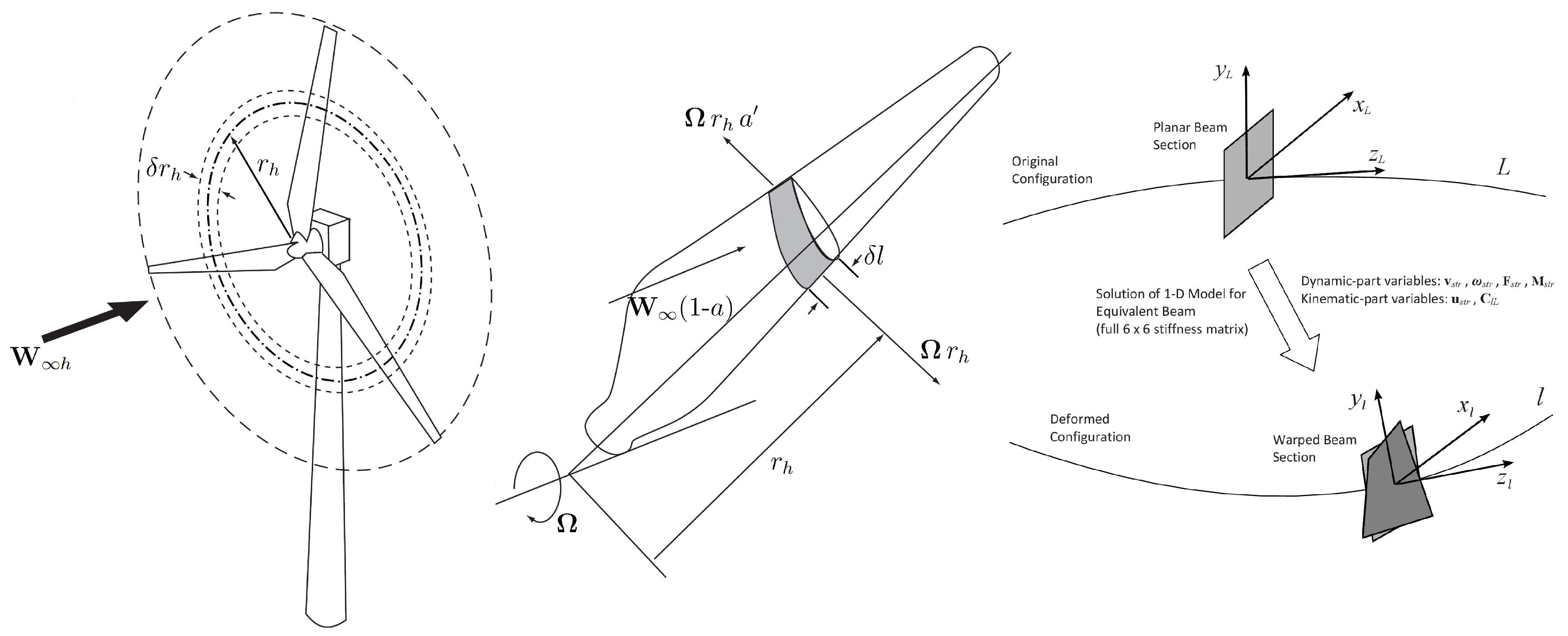
The motivation behind the DRD-BEM model are the limitations imposed by the underlying assumption in classical BEM that all blade sections are normal to the rotor’s radial direction. As a result of this, the blade section misalignments caused by rotor deformation are not properly represented. This misrepresentation becomes even more pronounced in case of large scale deformations, something that can be expected given the flexibility of modern blades. This issue is tackled by the Dynamic Rotor Deformation (DRD) part of the DRD-BEM. It ensures that in the DRD-BEM approach the rotor deformation is accurately represented owing to the action of a set of orthogonal matrices on the incident velocity and aerodynamic-force vectors. These matrix transformations account for all misalignments caused by various factors like deformation of blade sections, actions of mechanical devices controlling pitching, yawing or azimuthal rotation, changing winds, and several design features like coning or tilting of the rotor. Figure 1 shows schematically the instantaneous position of a blade element at distance from the hub. The radial thickness of the annular actuator swept by that blade element, in a coordinate system aligned with the hub, is given by . Also seen in that figure is the blade element’s spanwise length . As will be seen later, the DRD-BEM model judiciously uses these variables to ensure that all instantaneous misalignments are accounted for by constantly updating the area of the annular actuator corresponding to the respective blade element.
2.2. Structural Model: The Blade as a Complex Beam
The DRD-BEM models the structural response by using the Generalized Timoshenko Beam Model (GTBM). The GTBM is a generalized implementation of the Timoshenko beam theory using a variational asymptotic method. It accounts for warping of beam sections by interpolating sectional warping using a 2-D Finite element model to obtain 3-D warping functions. These warping functions are used to asymptotically approximate the 3-D strain energy at each section in terms of the six strain measures including those of the classical 1-D Timoshenko theory and the transverse shear in two directions. The complex geometry and material properties are represented by stiffness matrices obtained a priori for each section. The generalized implementation of the Timoshenko theory ensures a fully populated 6x6 stiffness matrix at each section of the beam coupling all 6 modes of deformation. The 3-D beam problem is thus reduced to a nonlinear 1-D beam. This unsteady nonlinear 1-D beam problem, together with the aerodynamic model, discussed later comprises the full aeroelastic scheme.
This aeroelastic scheme is solved along the beam’s reference axis, L, for every time step using an advanced ODE algorithm. From each time step of the ODE solution the 3-D fields can be recovered using the previously derived 3-D warping functions. As seen in Figure 1, the solution variables first represented in a coordinate system along L are transformed into the instantaneous coordinate system along the new configuration l. This is done with the help of the matrices, updated at every time step of the ODE solution of the structural model. Thus the instantaneous position of each blade section is accurately tracked by this intrinsic coordinate system. As a result the aerodynamic part of the aeroelastic analysis gets this updated information at every time step for each blade section. At the same time the results of the aerodynamic solution constantly update the aerodynamic loads acting at each blade section as inputs to the structural model for every time step.
2.3. The DRD-BEM Model
As mentioned earlier, a detailed description of the DRD-BEM procedure is presented in Ponta et al. [22]. The first step in the DRD-BEM procedure is to account for the effect of the annular actuator on the undisturbed wind velocity in the hub coordinate system, . First, the wind velocity which is originally given in a coordinate system aligned with the wind itself as is transformed to using a set of orthogonal matrices as follows
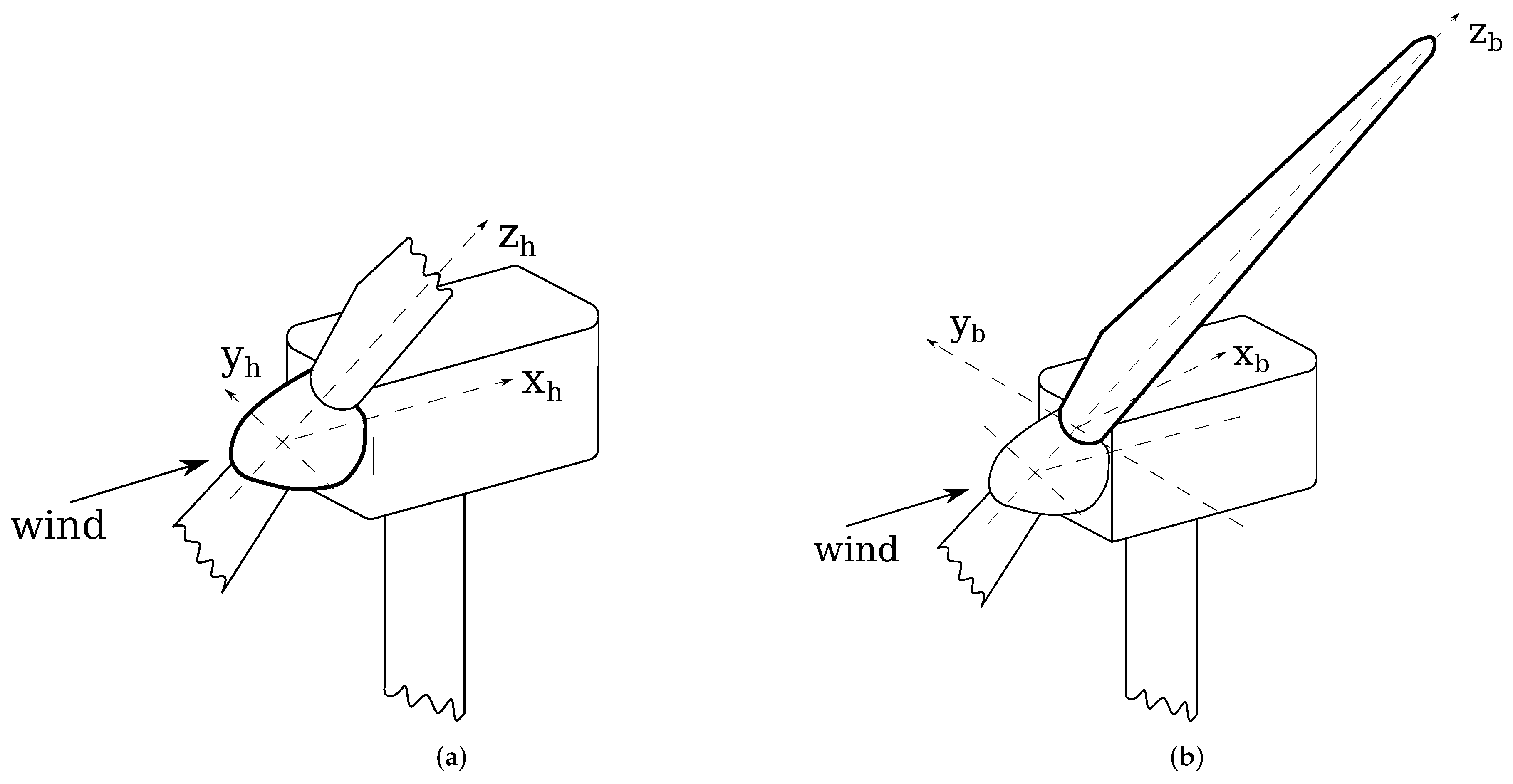
The first 2 coordinate transformations in Equation (1) represented by transformation matrices and account, respectively, for the misalignment at the nacelle due to yaw and the misalignment brought about by rotor tilt. The third orthogonal matrix, , rotates the blade around the main shaft to its new position at that instant transforming the wind velocity into the hub coordinate system h (see Figure 2a).
As this undisturbed wind flows across an annular actuator, it is deflected by the forces exerted on it by the actuator. Therefore, the wind velocity at the annular actuator, represented by , is given by,
where a and are the induction factors representing, respectively, the fraction of induced velocity in the axial and tangential directions of the hub coordinate system. , as shown in Figure 1, gives the instantaneous radial distance between the hub and the blade section in the hub coordinate and represents angular velocity of the turbine rotor.
is projected onto a coordinate system aligned with the blade section through a series of coordinate transformations. The first orthogonal transformation matrix is which accounts for coning and which performs a rotation about the blade’s pitch axis. This projects the wind onto blade coordinate system defined (see Figure 2b). projects the velocity vector onto the intrinsic coordinate system of the blade sections along the undeformed reference line L. Finally, is used to represent the undisturbed wind velocity in a coordinate system aligned with the instantaneous deformed configuration along reference line l. To get the final wind velocity as seen by the blade section we need to add two more components. First is the vibration velocities of that section as given by the structural model. The other component is the mechanical velocities, , accounting for yawing, pitching, azimuthal rotation or any other mechanical motion associated with that blade section. Since both these components are expressed in the l coordinate system, they can be added directly to the wind velocity obtained after all of the above mentioned coordinate transformations to give
The relative wind velocity magnitude in the plane of the blade section is given by . along with angle of attack are used to compute the aerodynamic lift and drag per unit length of that section giving the aerodynamic force vector
The aerodynamic load is then obtained in the hub h coordinate system by applying the inverse of the orthogonal matrices used earlier, this time, however, in the reverse order
Here projects the lift and drag forces onto the chord-normal and chord-wise directions in the l coordinate system.
This force is then equated with the forces obtained by performing the momentum balance in the hub coordinate system. The component normal to the annular actuator, , equated to the momentum change on and the tangential component , is equated to the momentum change on . An interference pattern is obtained, enabling us to use an iterative scheme to obtain the two induction factors a and . These induction factors are then used to obtain and then following all of the steps explained above compute the distributed aerodynamic forces on the entire blade per unit span length. gives the chord-normal and chord-wise aerodynamic loads and computes the aerodynamic moment around the first axis of l, per unit span length at each blade section. Here is the aerodynamic pitch coefficient of the airfoil at the corresponding angle of attack, is the density of air and c represents chord length of that section. The effect of gravity on the distributed forces and moments is also accounted for with the help of inertia properties of the equivalent beam represented by inertia matrices obtained as part of the GTBM process of dimensional reduction described in Section 2.2. These forces provide the input to the GTBM structural model.
2.4. Dynamic Update of Corrective Factors
To account for the various assumptions made in the blade element momentum theory certain correction factors have to be used. In DRD-BEM these factors, unlike the classical implementation of BEM, are updated dynamically. These include the rotational-augmentation effects as proposed by Du and Selig [33] and Eggers [34], dynamic-stall effects based on the works of Leishman and Beddoes [35,36,37], extrapolation of aerodynamic-coefficient data proposed by Viterna and Janetzke [38], tip and hub loss corrections (see Section 3.8.3 of Manwell et al. [26], and Ponta et al. [22]), and the tower-interference models proposed by Bak et al. [39] and Powles [40]. The DRD-BEM also incorporates the flexibility of multiple data sets for aerodynamic coefficients of different airfoils associated with factors varying the aerodynamic situation at the rotor. These factors could include varying Reynolds number, effects of flow control devices, etc.
2.5. The Glauert Correction
Another important modification needed in any model based on momentum theory is the correction of the thrust on the annular actuator when operating in the so-called turbulent-wake state. This correction, is the focus of the present paper, and plays a key role when the turbine operates at axial induction factors a greater than 0.5 (in practical implementations, this limit is lowered to about 0.3 to 0.45, depending on the corrective curve adopted).
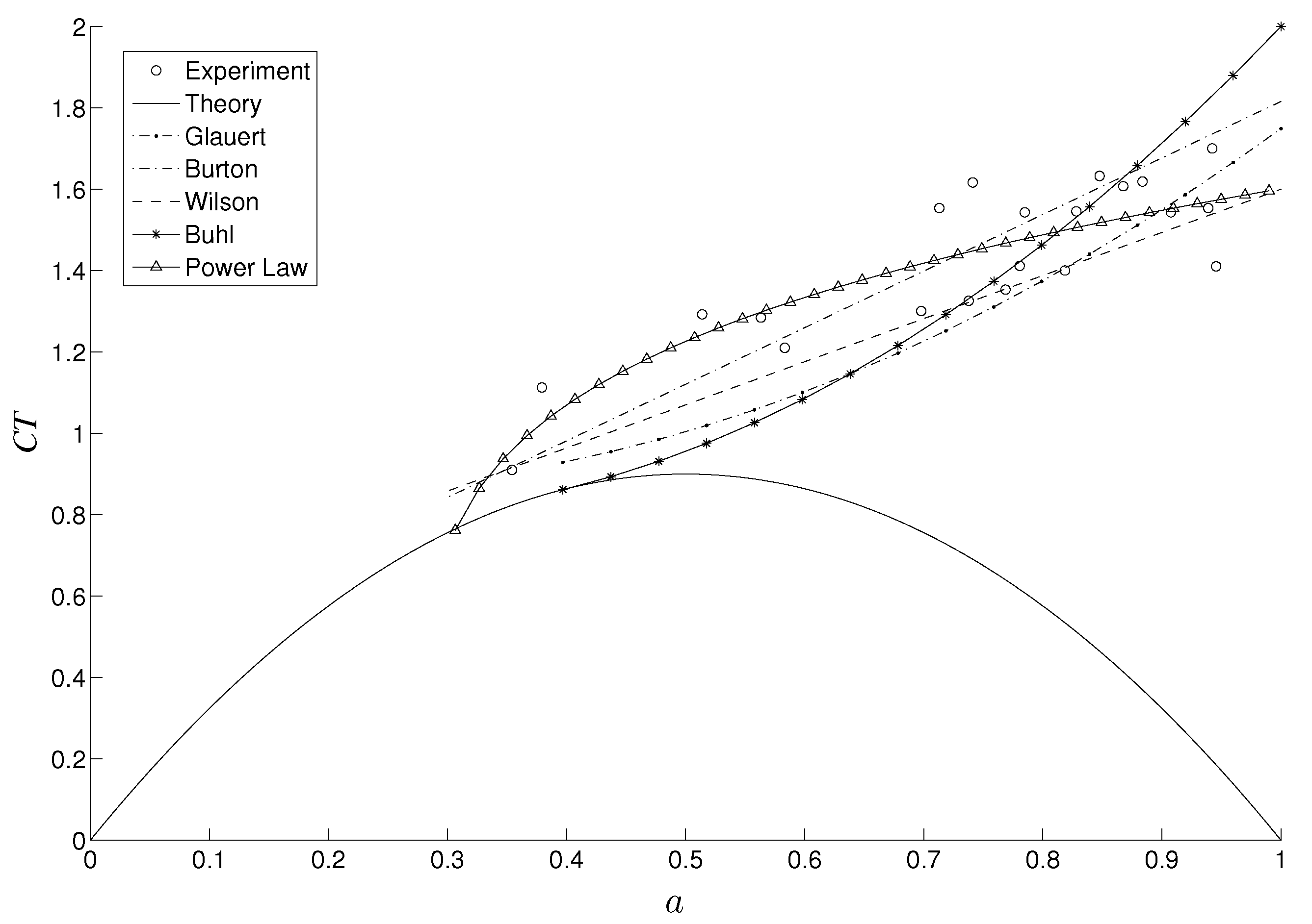
The classic streamtube-momentum solution for the actuator-disk representing the thrust coefficient as a function of a gives a parabolic curve of the form , which is depicted in Figure 3. At , that parabola reaches its vertex. Beyond that the basic assumptions of momentum theory on a streamtube control-volume become invalid, as the flow at the pseudo-infinite position, in the far wake downstream, would theoretically stagnate and start to propagate upstream. Physically, this flow reversal cannot occur, and what actually happens is that flow re-enters from outside of the wake, creating vortex structures and increasing the turbulent activity behind the rotor’s disk. This slows down the flow passing through the rotor, while the thrust continues to increase.
This work focuses on finding out a new extended empirical relation to compute the thrust for flow states with a high induction factor in the turbulent-wake state and the vortex-ring state. As explained in Section 1, instead of using momentum balance, Glauert [15] proposed finding from an empirical fitting to data from experiments on propellers provided by Lock and Townend [41]. As seen in Figure 3, Glauert’s empirical fit is tangent to the curve at . Alternative fitting functions to the same set of data were proposed by other researcher works like Wilson [21] and Burton et al. [20]. As noted by Buhl [19], a discontinuity between the function and the fitting curve can be observed upon the application of tip and hub losses. This makes convergence difficult to achieve for models where the induction factors are calculated iteratively. Buhl [19] solved the problem by using an empirical relation where the tangential match was enforced regardless of the tip and hub loss corrections. Another solution was proposed by Ponta et al. [22] in the form of a Power-Law fitting. The latter fitting curve, while significantly reducing the error of approximation, also avoids the discontinuity problem, since it always intercepts the stream-tube function whether or not the tip and hub losses are taken into account. The DRD-BEM model has the capacity to switch between any of these correction methods.
As mentioned in Section 1, the set of experiments reported by Lock and Townend [41] was recreated by numerically solving an actuator-disk set-up in ANSYS-Fluent. This numerical set-up also allowed to extend those experiments to the low interference conditions where , and regions of very-high values of interference factors in the vortex-ring state, characterized by , which go beyond the range of Lock and Townend [41] experiments. This new set of numerical data was then used to define a new empirical curve which can be used to find the thrust at high induction factor regimes. This new curve covers any induction factor between and , and merges seamlessly with the versus a curve from the streamtube theory for values of . The following sections discuss the set of numerical experiments performed, together with the analysis of physical aspects associated with the actuator-disk model operating at flow states with high induction factors.
3. The Physics of the Actuator Disk Model
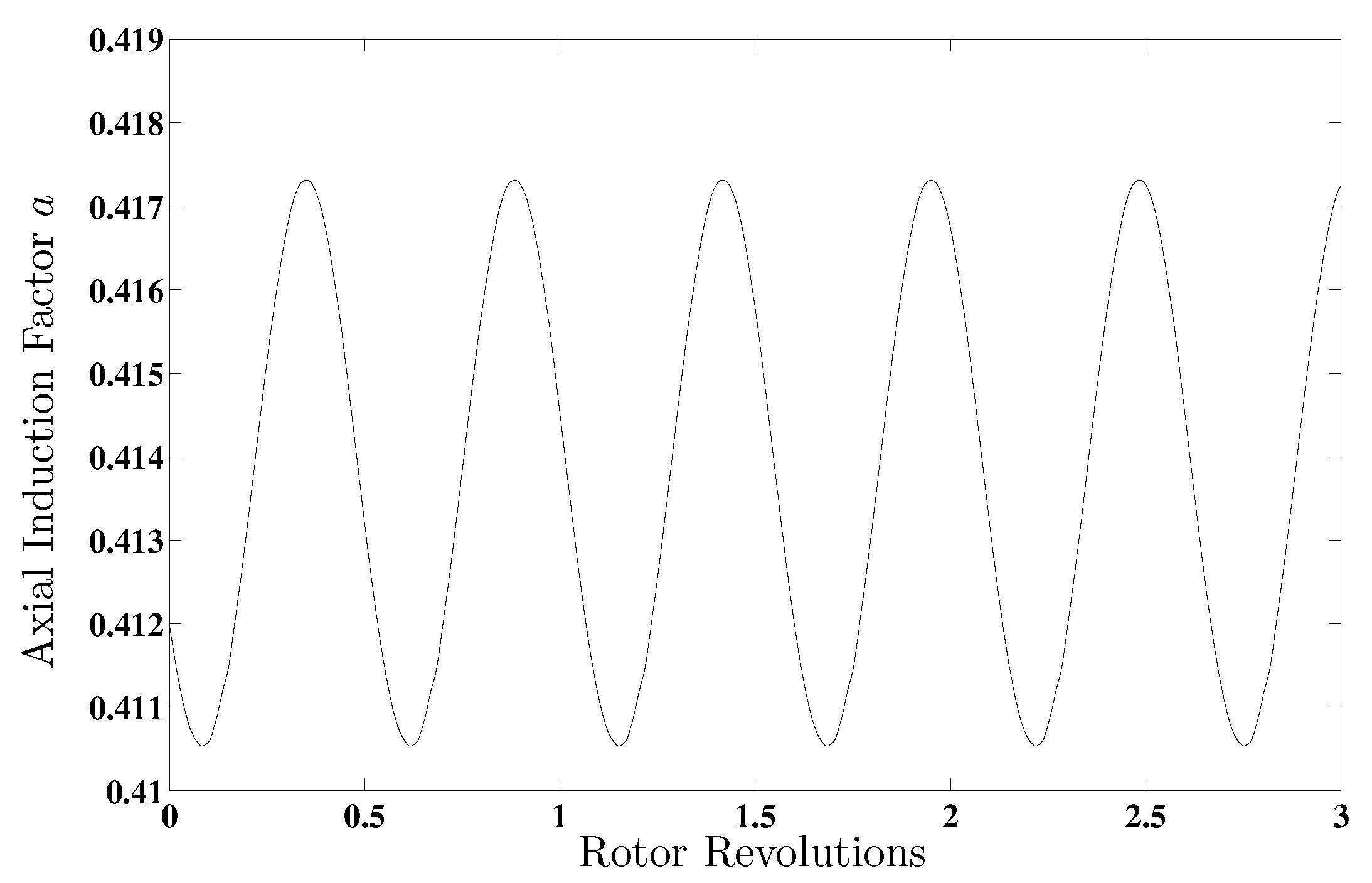
As it was mentioned in previous sections, future turbines are expected to undergo larger levels of deformations, which in turn will induce higher levels of misalignment of the airfoil blade sections which respect to the incoming flow (see Otero and Ponta [42] for a detailed description of blade-section misalignment effects). These misalignments lead to changes in the effective interference at the rotor annular areas swept by those misaligned blade sections, often leading to higher axial-induction factors at various portions of the rotor. The nature of the DRD-BEM model is such that it captures these misalignments with great accuracy. This means that the simulation will detect flow states not lying in the standard operating regimes more precisely. As an example, we shall analyse such a possible scenario based on a DRD-BEM simulation of the benchmark NREL-5MW RTW turbine. Figure 4 shows simulation results of a de-loaded NREL-5MW turbine operating in the control region at a wind speed of 8 m/s, where the turbine is optimized for power extraction [24]. The turbine is de-loaded by increasing the rotor RPM from approximately 9.2 rpm to 15 rpm to obtain a 10% margin of reserve power from the turbine. Jonkman et al. [24] gives the range of optimal rpms for an NREL-5MW turbine with varying wind speeds. A power reserve of 10% is based on Ahmadyar and Verbič [43] which analyses de-loading an NREL-5MW reference turbine and also on Venne et al. [44] and Chang-Chien et al. [45] where control strategies based on de-loading the turbine along with realistic limits of rpm variation used for such strategies are analyzed. An axial induction factor greater than can be observed and this, as it was mentioned before, lies in the turbulent-wake state, and requires the application of the Glauert correction.
3.1. The Experimental Data
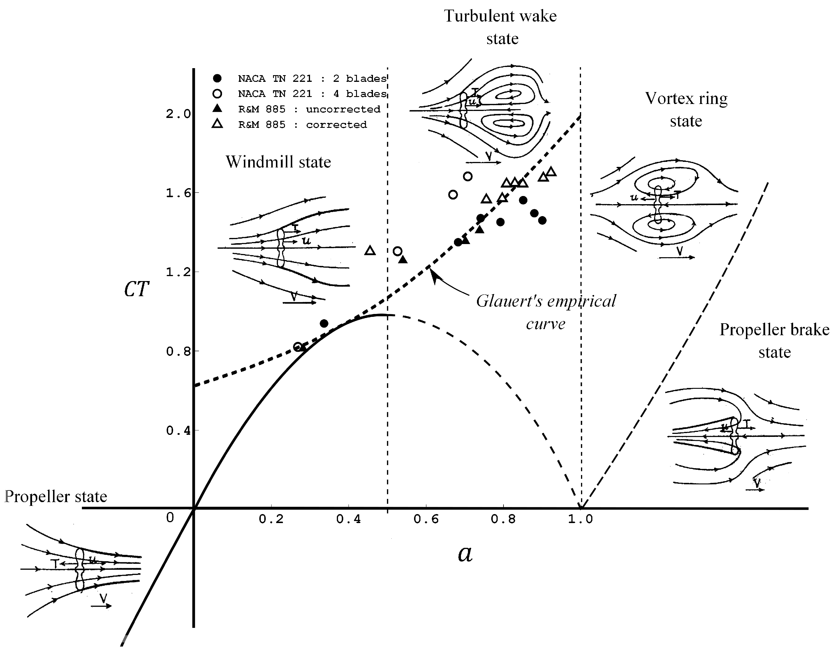
As the axial induction factor varies, the rotor goes through several interference states. Figure 5 depicts the different states as compared to the theoretical parabolic curve obtained by the momentum theory. The experimental results used by Glauert [15] are also plotted.
For values of , the rotor acts as a regular propeller, transferring energy to the flow instead of extracting energy from it, with a negative thrust (e.g., with the thrust pointing in the upwind direction).
The normal operating state of the wind-turbine rotor, known as the windmill-brake state, is where the rotor maximizes energy extraction from the flow. In particular, the ideal condition occurs where the axial induction factor a is equal to , which is characterized by a power coefficient (or approximately 59.26%). This represents an optimum value of energy-conversion efficiency for an ideal wind-energy harvester, usually referred to as the Betz’s limit (in honour of German physicist Albert Betz who proposed the analysis in 1919 [20,26]). Wind-turbine designs target this ideal as their nominal (or “rated”) operational conditions. Betz’s ideal condition lies within the windmill-brake state.
With an increase in tip speed ratio either due to a drop in wind velocity, a change in the turbine’s rotational speed, or a change in rotor orientation with respect to the wind, the axial load on the rotor disk increases in proportion to the wind velocity. This leads to an increase in the axial induction factor. Initially there is incipient recirculation in the rotor’s wake with re-entrance of flow from outside of the wake, which mixes with the slow moving wake flow. This is the so called turbulent-wake state that we described before. In terms of the actuator-disk analogy, in this state the rotor disk begins to act like a semi-porous imaginary surface with decreasing permeability. As seen in Figure 5, the turbine is said to be in this state when the axial induction factor a lies approximately between 0.5 and 1. The experiments reported by Lock et al. [16] are one of the earliest studies of high interference states where the author goes on to propose a possible empirical correction. Several others have provided a detailed analysis of the high axial induction factor regimes. These include Burton et al. [20], Stoddard [48,49], Eggleston and Stoddard [46], and Wilson and Lissaman [50]. In particular Glauert [15] forms the basis of the correction model used in BEM. More recent are the works of Sørensen et al. [51] presenting a numerical analysis of an actuator disk model in this regime, and Johnson [23] presenting a detailed analysis of several noteworthy experiments that have provided data for these flow states.
For values of a higher than 1, the rotor enters the vortex-ring state, where the recirculation starts to assume a toroidal pattern approximately centered at the rotor’s disk. As a increases beyond 1, the flow direction across the rotor starts to reverse. In this condition the turbine acts like a propeller operating in brake mode (that is the case of a propeller aeroplane in the landing run after touching down), and begins to transfer energy into the flow with an increased thrust in a downwind direction. This flow state is referred to as the propeller-brake state.
3.2. The Numerical Approach
As mentioned previously, this experimental approach has been the most widely accepted method to account for rotor interference in high a regimes, with relatively slight modifications introduced to improve Glauert’s original empirical relation. One factor to point out is the substantial amount of dispersion seen in the experimental data used by Glauert. This could be attributed to the limitations of the sensors from that era, as well as, to the unsteady nature of the flow in the close surroundings of a real rotor. On the other hand, the interference computation in BEM theory is based on an idealization steady-in-the-average evaluation of the momentum change in a streamtube control-volume, which differs from the situation across a real rotor.
However, it can be argued that an actuator-disk model is still a very suitable representation of the rotor interaction with the flow, and that is the main reason the method has been widely employed for so many years. Therefore, Glauert’s basic concept of replacing the momentum balance in the streamtube by a mathematical expression giving a functional relation of versus a (that represents a more complex turbulent-flow interference) is still valid. Moreover, several recent experimental studies on actuator-disk models have been carried by Castro [52], Hong [53], Lignarolo et al. [54], Batten et al. [55], and Harrison et al. [56]. These studies, however, concentrate mostly on wake analysis instead of the analysis of conditions at, or in the close surroundings of the disk, which is what is needed for a BEM model.
Wake measuring experiments benefit from the fact that non-steady effects created in the near surroundings of the rotor get attenuated by the distance. On the other hand, measuring flow properties in the close surroundings of the rotor’s disk is much more challenging. Thus, for conditions at the actuator itself, a numerical analysis would be better suited, as the actuator-disk is essentially an imaginary semi-porous surface that induces a pressure drop. These conditions are relatively easy to set-up in a numerical simulation.
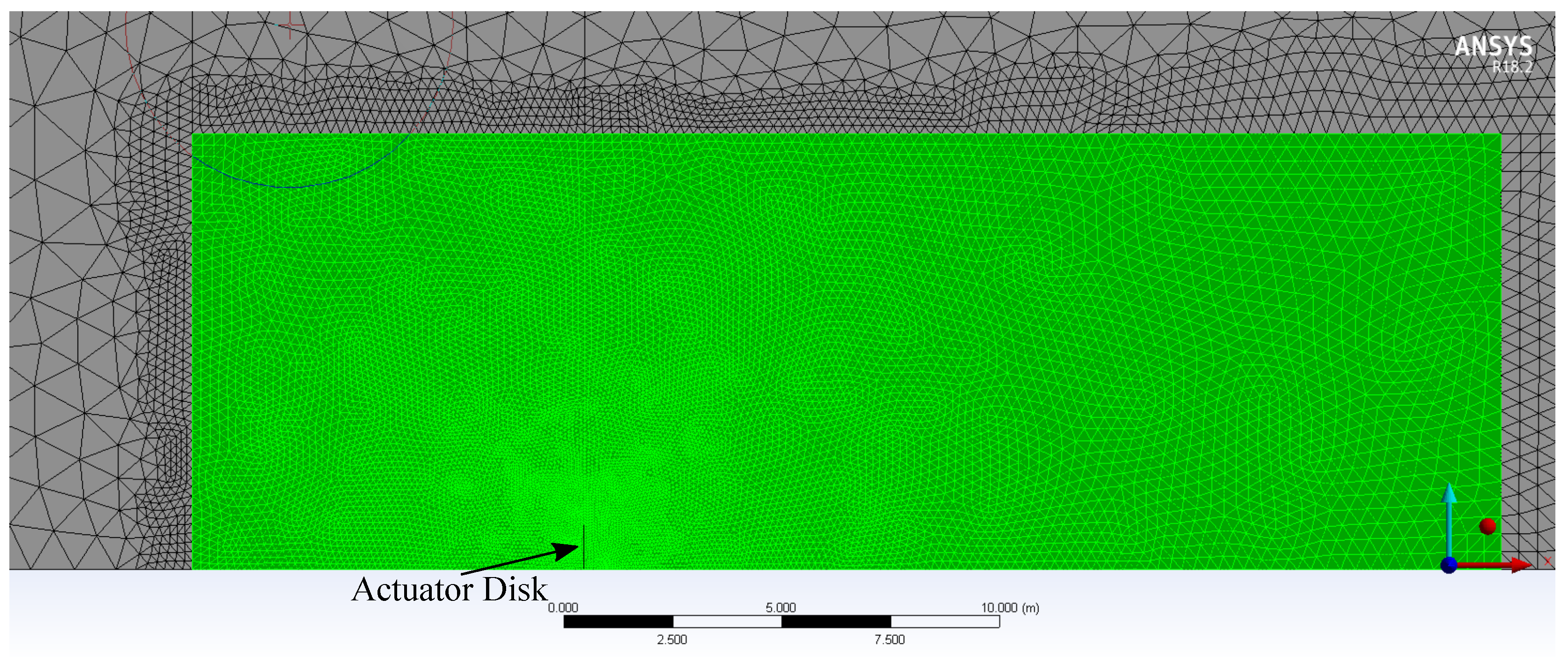
The numerical model has been developed in ANSYS-Fluent. It consists of a 1m radius actuator disk in a 2-D axisymmetric domain. The disk is essentially an infinitesimally thin boundary lying at an interface across cells. This infinitesimal interface represents an actuator disk by virtue of a discontinuous pressure drop acting across it. For this experiment, the acting on the disk was varied by varying this pressure drop. A relatively large domain size was selected to ensure that the external boundaries do not affect the solution at the actuator disk, especially when the flow enters the extremely unstable vortex ring state. The overall domain size was 250 m upstream and 350 m downstream of the actuator disk and extended 400 m above the horizontal axis of symmetry. Figure 6 shows a close-up view of the the local domain surrounding the actuator-disk region in one of the meshes used in this study.
The typical boundary conditions of Velocity inlet and pressure outlet were used for the external boundaries. A free-stream velocity, U, of 1 m/s was used. An unstructured triangular mesh using the ANSYS meshing tool was used to discretize the domain. The gradient adaption algorithm of Fluent was used to dynamically refine the mesh at each iteration using the curvature of velocity as the refinement criteria.The Navier-Stokes equations for the turbulent flow across this disk were solved in this discretized domain by adopting a turbulence model of the family called the realizable. As explained in ANSYS [57] and Menter [58], the family of models are based on the evaluation of two properties of the turbulent flow: the turbulence kinetic energy k, and its dissipation rate . The models are more suitable to simulate turbulent properties on the far-field flow regions than other turbulence models like the ones in the family. That is why the SST model gradually changes from a approach in the boundary layer to a formulation in the free-shear regions. It can be reasoned that the actuator disk, because of its semi-porous surface nature, mostly deals with free-shear effects at the zone of interaction between the disk and the incident flow than with near-wall type conditions, therefore, a model was chosen.
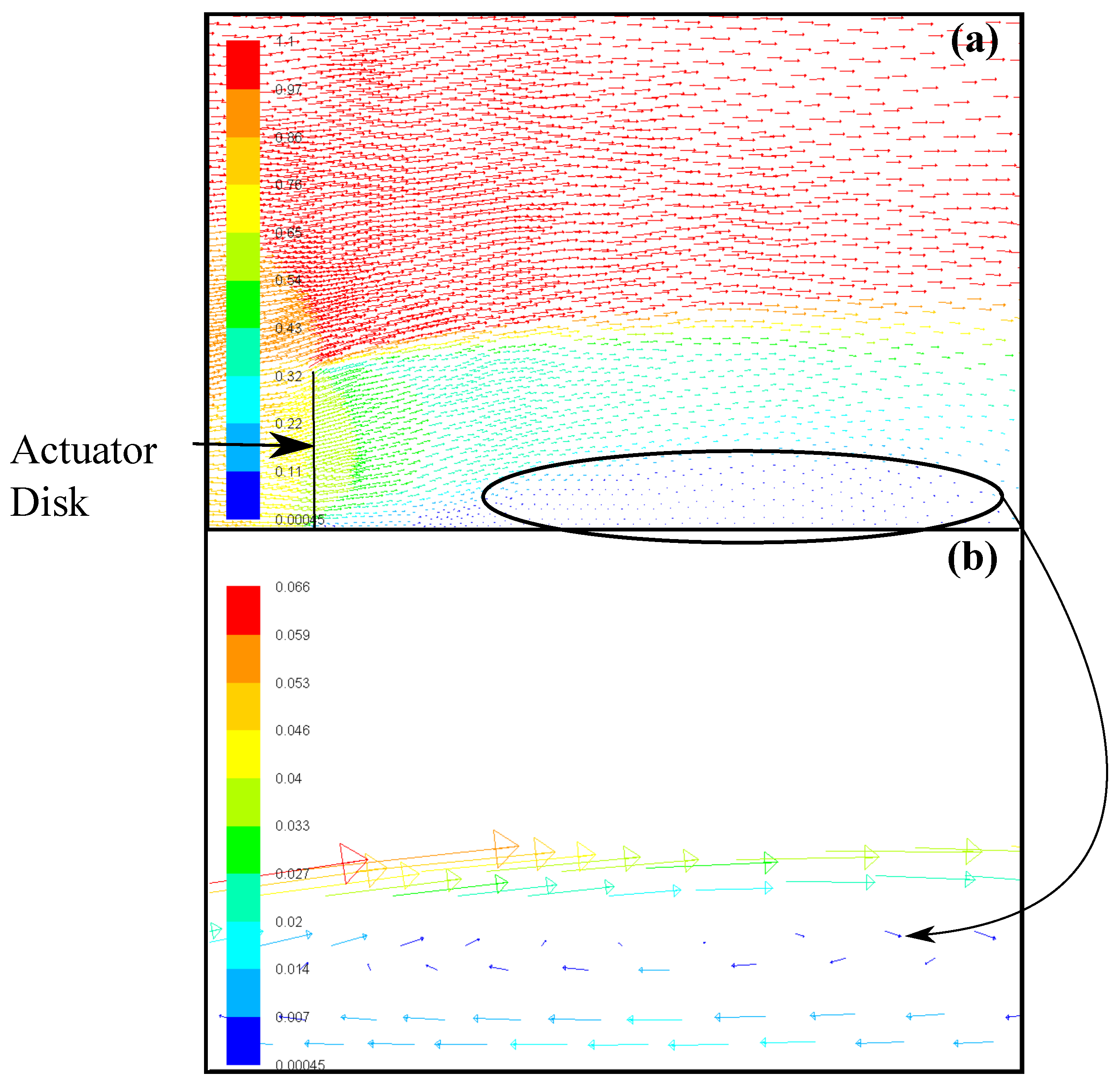
In particular for the case of boundary-free shear flows with high mean shear rate, and also for flows with secondary flow features, the realizable version of the model performs better than other models of the family [57,59]. These are the flow conditions expected from the actuator-disk model, which are characterised by a sudden pressure drop. A thorough comparison was carried out between the realizable model with the other turbulence models available in Fluent. The flow topology observed in the simulations supports the use of a realizable model. Figure 7 shows an expanding wake behind the actuator disk for an axial induction factor with . The first signs of vortical wakes with recirculating patterns and re-entry flow can be seen in the zoomed-up view in Figure 7b. This pattern is absent in the simulation results for . As explained earlier, this flow pattern signals the beginning of the turbulent-wake state, on which the streamtube control-volume theory is no longer applicable to the actuator disk model. Significantly, that is precisely the region around which the experimental data compiled in Glauert [15] start to enter the turbulent wake state (see Figure 3).
Furthermore, it was seen that results from the realizable model best matched the data used by Glauert for flow in the turbulent-wake state. It also closely follows the trend of the power-law fitting proposed in Ponta et al. [22] in the region lying between the turbulent-wake state and the vortex ring state. This power-law fitting has previously been shown to minimize the approximation error to the experimental data used by Glauert [15]. Another indication of the the realizable model’s suitability is the fact that the simulation results at low axial interference factors (i.e., ) matches perfectly with the theoretical solution for the streamtube control-volume analysis in classic BEM theory. The streamtube analysis for such low-interference flow regimes has been validated in numerous studies involving both, controlled experiments on propellers and scaled-down turbine models, as well as field measurements on full-scale turbines. All these observations validate the use of the realizable model to solve the actuator disk flow in our numerical experiments.
The values for the pressure drop applied across the actuator disk in the simulations were computed from the coefficient of thrust expected for the operational range under study. is given by:
where A is the area of the actuator disk, the air density, U is the free-stream velocity equal to 1 m/s and T the thrust on the disk, which could be written in terms of the pressure drop as . Therefore, the relation for pressure drop across the actuator disk is given by:
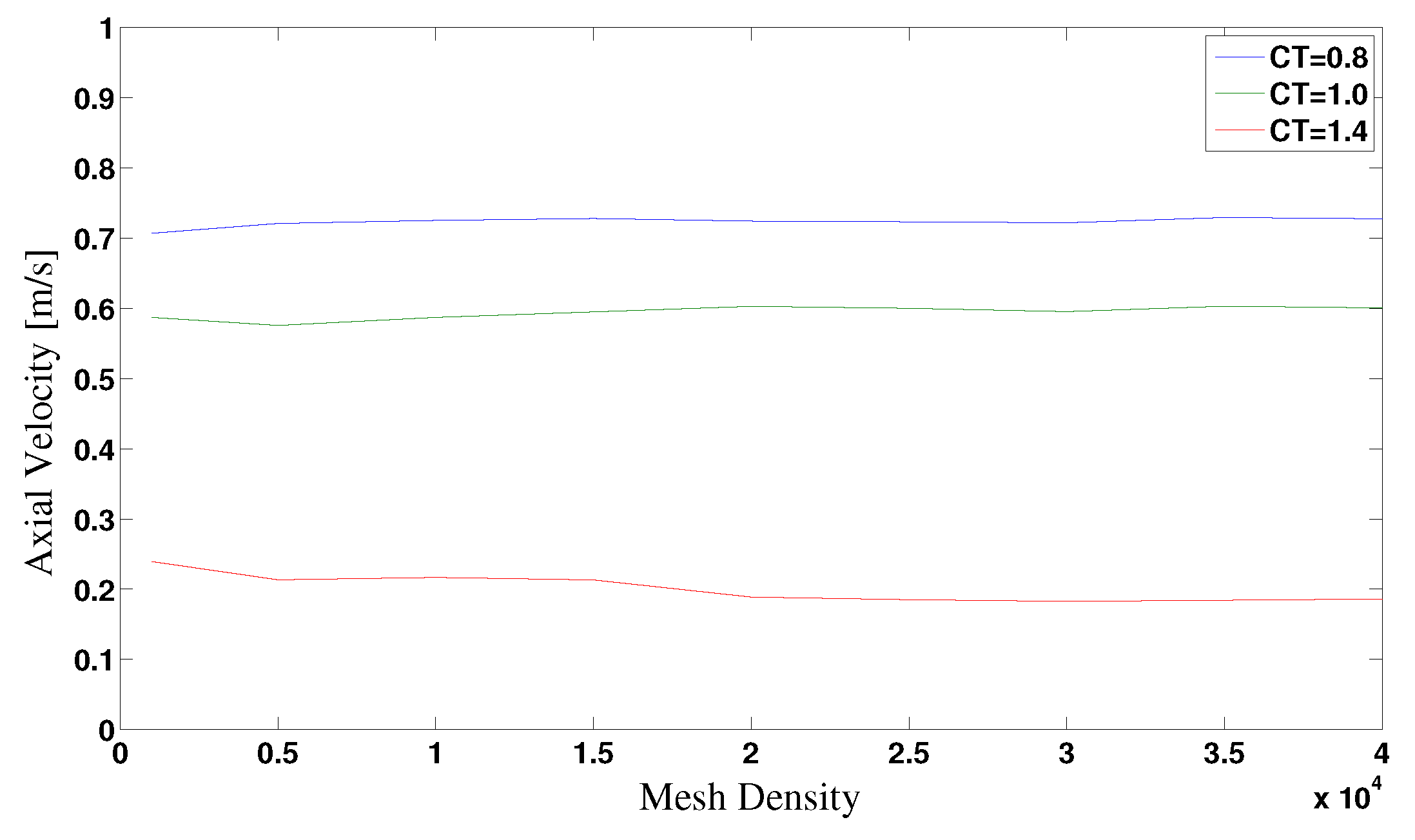
Before applying the the numerical model to obtain the new set of data, we conducted a thorough test to confirm that the final mesh obtained by using Fluent’s gradient adaption algorithm consistently resulted in an accurate solution. To this end, a mesh convergence analysis was performed on three points selected from the curve shown in Figure 3. The values selected for the mesh convergence analysis were , 1 and . This can be seen in Figure 8, which shows a plot of axial velocity at the disk against the mesh density. These cases cover flow states ranging from low axial induction factor windmill brake states to the point were the flow in the turbine wake is well into the turbulent wake state.
The mesh density was varied using two meshing parameters: The Global mesh refinement and the element growth rate around the disk. To vary the growth rate in the proximity of the disk a smaller local domain around the disk was selected within the larger global domain. This domain extended 21 m downstream and 9 m upstream of the disk and 10 m above the axis of symmetry. As a result the increase in element count was observed primarily in the local domain, thereby, avoiding an unreasonably dense mesh in the entire domain. This would increase solution times exponentially without any contribution to solution accuracy, given that outside of the local domain, the flow can be considered as free stream. The criteria for mesh convergence was set at a velocity residual lower than 0.01 m/s between successive mesh refinements. The number of elements was increased from approximately 1000 elements to 40,000 elements, within the local domain of the disk, in steps of approximately 5000 elements. As an example, the local domain highlighted in green in Figure 6 shows a particular refinement of approximately 20,000 elements, with the global domain consisting of 35,000 elements.
It was observed that solution reached the above mentioned convergence criteria within the first couple of refinements for all three values. Finally, these axial velocities were compared against those obtained using the Gradient Adaption algorithm in Fluent. The difference in velocities was well within the 0.01 m/s criteria mentioned above. It was, therefore, decided to go ahead with Fluent’s Gradient Adaption method.
Finally, the axial induction factor a was computed from the average flow velocity across the actuator disk obtained from the simulations using the relation , where U is the free-stream velocity, and is the area-weighted average of the axial velocities at the interface representing the actuator disk. The axial induction factors were plotted against their respective values to obtain the new correction curve.
4. The New Polynomial Correction Curve
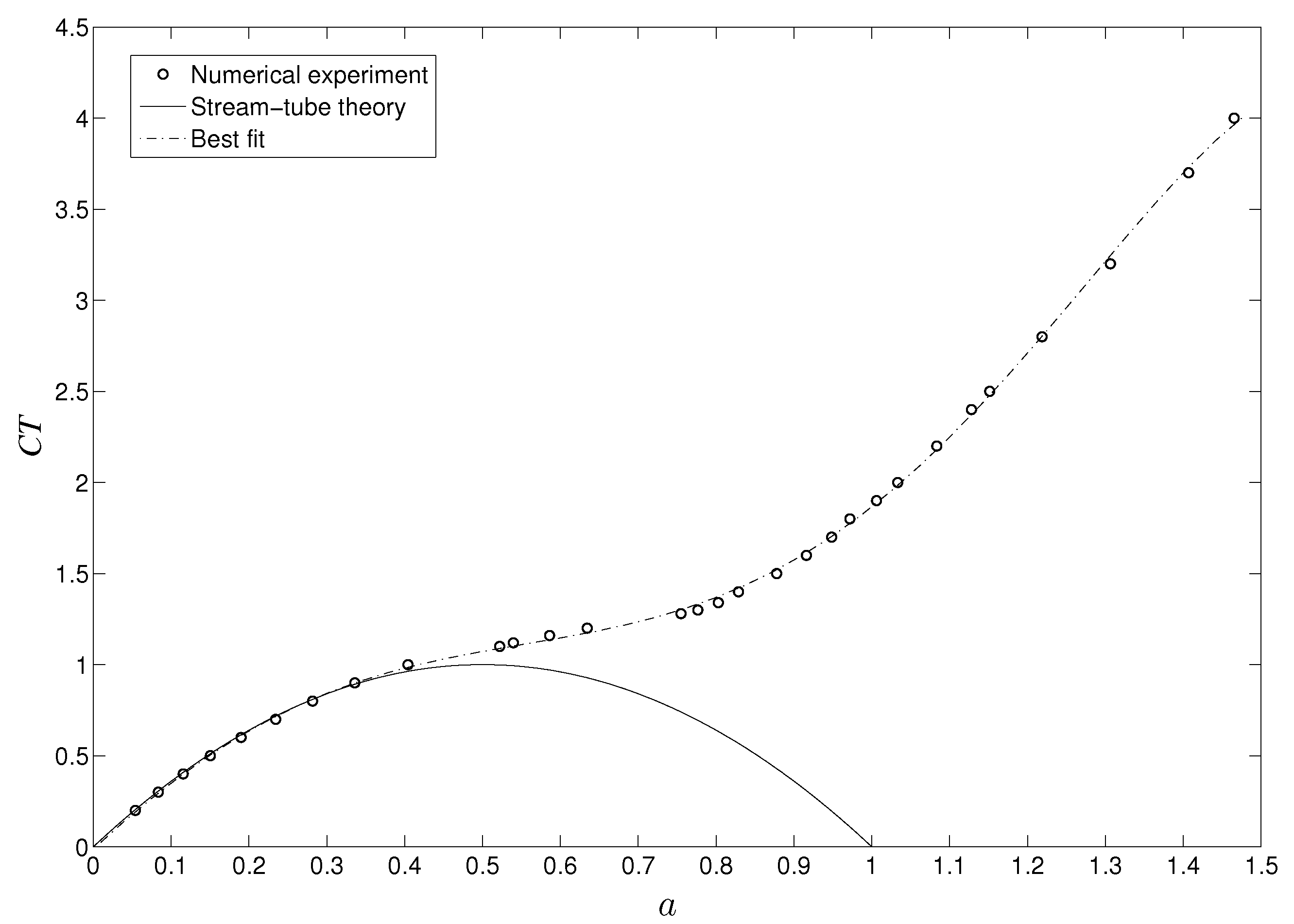
Figure 9 shows the numerical results for the versus a relation obtained from the numerical experiments previously described, together with a best-fit curve to the data obtained by a least-squares regression of a 4th order polynomial, and the parabolic relation given by the classic streamtube momentum solution. As it could be seen, the numerical experiments not only merge smoothly with the classic streamtube-momentum solution, but also shows a very close agreement with the classic curve all over the range of values where the classic theory is valid.
A very important issue that needs to be considered for any versus a correction method that is proposed, is the merging of the correction curve with the streamtube-momentum parabola. In particular, as previously mentioned in Section 2.5, how this merging may produce discontinuities that may affect convergence of the iterative process in the BEM solution when the tip and hub loss factors are taken into account (for a detailed description on subject of tip and hub loss factors see Section 3.8.3 of Manwell et al. [26], and Ponta et al. [22]). In this regard, determining the point of departure of the polynomial fitting curve from the theoretical parabolic curve is worth of further consideration.
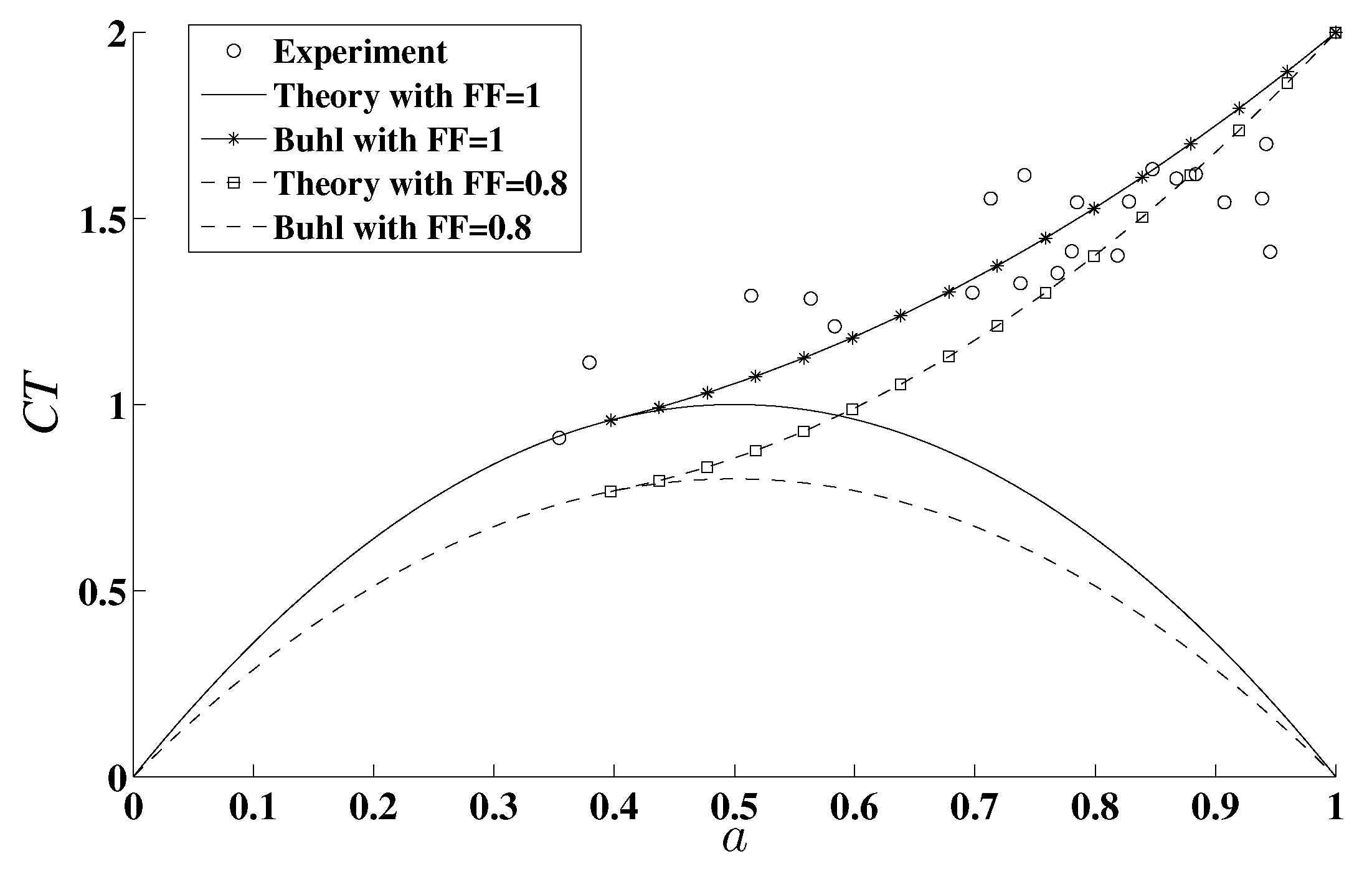
As it was discussed in Section 2.5, Glauert’s original empirical fit was designed to be tangent to the curve at , which as noted by Buhl [19], creates a discontinuity between the theoretical parabolic function and the correction curve when tip and hub loss factors are applied. Buhl [19] solved the problem by proposing an empirical relation where the tangential match was enforced at regardless of the tip and hub loss corrections. In that process, the initial data points from Glauert’s experimental data set are essentially ignored, and the adapted correction curve is set as a parabola that fits the tangential merging at , and it is anchored in its other end at curve at . This procedure is illustrated in Figure 10, where Buhl’s fitting without tip-hub losses is compared with a fitting incorporating a tip-hub loss factor of (another example with can be seen in Figure 3). Buhl [19] method is successful in avoiding the convergence problem associated with the discontinuity in the versus a curve, but it has the caveat that as decreases, the resulting curve does not match the trend of the experimental data (which could be seen in Figure 10), and the error of approximation increases.
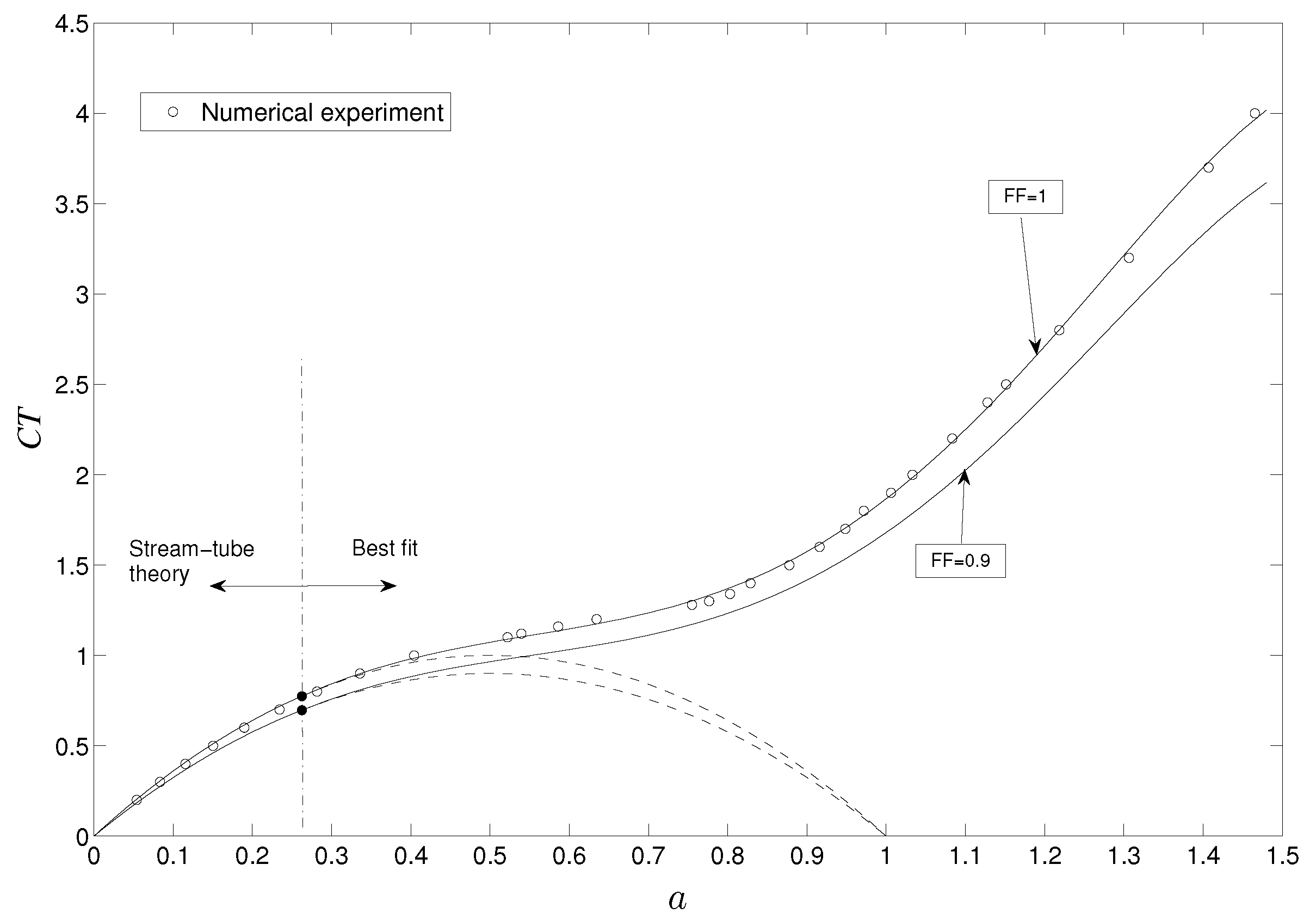
Upon a closer examination of the origin of the tip-hub losses, an alternative approach can be proposed. Even though in BEM theory the factor is applied to the momentum change in the streamtube wake, the tip-hub losses are, actually, physically associated with the trailing vortices created at the tip and root of the rotor blades, in the same way that they form at the tip and root of an airplane wing. That means that the origin of this effect is connected with the Blade Element part of the BEM theory, and as such, the effect is still going to be present even if the rotor goes beyond the range of the windmill-brake state and enters the turbulent-wake state. Therefore, shifting the entire fitted curve in accordance with the tip-hub loss factor, as it is done with the theoretical parabolic relation, seems like a logical option. By fitting the polynomial curve using the entire data set all the way from to , and not just after , and then applying the factor, we ensure that the curves always merge gradually in the range between and . It also ensures that the accuracy of the streamtube analysis, validated many times, is effectively used. In the practical implementation in the context of the DRD-BEM model, we adopted as the switching point between the two curves, with the theoretical curve covering the range of , and the polynomial fitting the range of . Figure 11 shows examples of the polynomial correction curve for the case of no tip-hub losses, and for the case of a tip-hub loss factor .
Implementation in the Context of the DRD-BEM Model
To test the performance of the new polynomial-curve correction, we incorporated it into the general scheme of the DRD-BEM model. We conducted simulations based on two operational scenarios for the NREL-5MW turbine. Both scenarios are characterized by values of the axial induction factor a higher than 0.4 on the blade section located at 90% of the span (i.e., the rotor is operating within the turbulent-wake state).
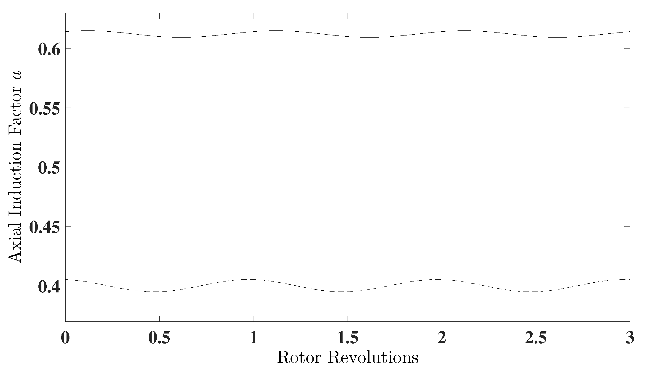
Of the two scenarios, the first one represents a typical situation during the start-up regime of an NREL-5MW, as reported by Jonkman et al. [24], with a rotor’s angular speed of 7.9 rpm and a wind velocity of 6 m/s. The mean a over 3 rotor revolutions is found to be 0.403. The second scenario represents the situation of an NREL-5MW turbine rotating at its nominal speed of 12.1 rpm, with the wind velocity dropping suddenly from the nominal velocity of 11.4 m/s to 5.8 m/s. The mean a over the same 3 cycles is 0.612. A comparison of the time evolution of the axial induction factors for the two test cases can be seen in Figure 12.
5. Conclusions
In this paper, a new evolution of the BEM theory for wind turbines operating in high axial interference regimes is presented. This analysis is based on numerical experiments on an actuator disk model. A primary reason for exploring these operational regimes is the increasing complexity of wind turbine control strategies, and the increasing complexity of the structural response of wind turbine blades. This has resulted in wind turbines often operating at regimes not usually found earlier. With state of the art and future turbine blades experiencing higher levels of deformation, flow states at higher axial induction factors are (and will be) encountered more frequently and for longer durations. Figure 4 and Figure 12 show the examples of test-case simulations where the turbine does, in fact, enter such a flow state. An important motivation for this exploration is the ability of the DRD-BEM model to capture the complex nature of dynamic rotor deformation, with the resulting misalignment of the blade airfoil sections with respect to the incident flow, and its subsequent effects on the aerodynamic forces. This feature gives the DRD-BEM a capacity to detect a wider range of induction factors, improving turbine performance predictions at a wide variety of operational regimes.
A full analysis of the flow across an actuator disk, based on a turbulent Navier-Stokes solution by the realizable model, was conducted in ANSYS-Fluent for operational regimes covering a wide variety of axial induction factors. Results from these numerical experiments for the versus a curve are in good agreement with the experimental data set used by Glauert [15], and are also in excellent agreement with the parabolic curve given by the classic streamtube control-volume theory all over the range where it is valid. Figure 5 and Figure 9 show how both Glauert’s data set as well as the present numerical results start departing from the theoretical curve at approximately to . Also, the sudden increase in in the experimental data, as seen in Figure 3, coincides with the appearance of wake recirculation in the numerical model (see Figure 7, and the discussion associated with it), which supports the validity of the numerical model used in this work.
A 4th order polynomial regression was proposed to fit the numerical data obtained by the numerical model. This new fitting curve was introduced in the context of the DRD-BEM model to compute for axial induction factors a higher than . An important observation that can be made on the Glauert [15] correction (and indeed for any other previous correction proposed since) is that it does not include the vortex-ring or the propeller-break states starting at around . The new polynomial curve proposed here extends the correction all the way upto for the first time, covering regimes that were not covered previously. Hence, this study extends the capacities of BEM models in general, and the DRD-BEM model in particular to the analysis of situations beyond . For the reasons mentioned before, it can be expected to see this operational flow regimes gaining in importance with the turbines of the future. Thus, it can be said that the study presented in this work fills an important gap in the available modeling resources for wind turbine performance and dynamics.
Author Contributions
Conceptualization, A.R. and F.L.P.; methodology, A.R. and F.L.P.; software, A.R. and F.L.P.; validation, A.R. and F.L.P.; formal analysis, A.R. and F.L.P.; investigation, A.R. and F.L.P.; resources, A.R. and F.L.P.; data curation, A.R. and F.L.P.; writing—original draft preparation, A.R. and F.L.P.; writing—review and editing, A.R. and F.L.P.; visualization, A.R.; supervision, F.L.P.; project administration, F.L.P.; funding acquisition, F.L.P.
Funding
This research was funded by the United States National Science Foundation through grant CEBET-0952218.
Conflicts of Interest
The authors declare no conflict of interest.
References
- NREL. 20% Wind Energy by 2030: Increasing Wind Energy’s Contribution to US Electricity Supply; Technical Report DOE/GO-102008-2567; US Department of Energy: Washington, DC, USA, 2008.
- Corbetta, G.; Pineda, I.; Wilkes, J. Wind in Power—2013 European Statistics; European Wind Energy Association: Brussels, Belgium, 2014. [Google Scholar]
- Jamieson, P. Innovation in Wind Turbine Design; Wiley: Hoboken, NJ, USA, 2011. [Google Scholar]
- EWEA. Wind Energy’s Frequently Asked Questions, 2016. Available online: http://www.ewea.org/wind-energy-basics/faq/ (accessed on 28 April 2017).
- Campbell, S. 10 of the Biggest Turbines. Wind Power Monthly, 2016. Available online: http://www.windpowermonthly.com/10-biggest-turbines (accessed on 28 April 2017).
- Ponta, F.L.; Otero, A.D.; Rajan, A.; Lago, L.I. The adaptive-blade concept in wind-power applications. Energy Sustain. Dev. 2014, 22, 3–12. [Google Scholar] [CrossRef]
- Muljadi, E.; Butterfield, C.P. Pitch-controlled variable-speed wind turbine generation. IEEE Trans. Ind. Appl. 2001, 37, 240–246. [Google Scholar] [CrossRef] [Green Version]
- Geng, H.; Yang, G. Linear and Nonlinear Schemes Applied to Pitch Control of Wind Turbines. Sci. World J. 2014, 2014, 406382. [Google Scholar] [CrossRef] [PubMed]
- Dvorkin, Y.; Ortega-Vazuqez, M.; Kirschen, D. Wind generation as a reserve provider. IET Gener. Transm. Distrib. 2015, 9, 779–787. [Google Scholar] [CrossRef]
- Sun, Y.Z.; Zhang, Z.S.; Li, G.; Lin, J. Review on frequency control of power systems with wind power penetration. In Proceedings of the 2010 International Conference on Power System Technology (POWERCON), Hangzhou, China, 24–28 October 2010; pp. 1–8. [Google Scholar]
- Lubosny, Z.; Bialek, J.W. Supervisory Control of a Wind Farm. IEEE Trans. Power Syst. 2007, 22, 985–994. [Google Scholar] [CrossRef]
- Tang, X.; Fox, B.; Li, K. Reserve from wind power potential in system economic loading. IET Renew. Power Gener. 2014, 8, 558–568. [Google Scholar] [CrossRef]
- Muljadi, E.; Singh, M.; Gevorgian, V. Fixed-speed and variable-slip wind turbines providing spinning reserves to the grid. In Proceedings of the 2013 IEEE Power and Energy Society General Meeting (PES), Vancouver, BC, Canada, 21–25 July 2013; pp. 1–5. [Google Scholar]
- Sebastian, T. The Aerodynamics and Near Wake of an Offshore Floating Horizontal Axis Wind Turbine. Ph.D. Thesis, University of Massachusetts—Amherst, Amherst, MA, USA, 2012. [Google Scholar]
- Glauert, H. The Analysis of Experimental Results in the Windmill Brake and Vortex Ring States of an Airscrew; Technical Report Reports and Memoranda Volume 1026; Great Britain Aeronautical Research Committee: London, UK, 1926.
- Lock, C.N.H.; Bateman, H.; Townsend, H.C.H. An Extension of the Vortex Theory of Airscrews With Applications To Airscrews of Small Pitch, Including Experimental Results; Reports and Memoranda No. 1014; British Aeronautical Research Committee: London, UK, 1926.
- Lock, C.N.H.; Bateman, H. Some Experiments on Airscrews at Zero Torque, with Applications to a Helicopter Descending with Engine “Off”, and to the Design of Windmills; Reports and Memoranda No. 885; British Aeronautical Research Committee: London, UK, 1924.
- Munk, M.M. Model Tests on the Economy and Effectiveness of Helicopter Propellers; Technical Report TN-221; NACA: Washington, DC, USA, 1925. [Google Scholar]
- Buhl, M. A New Empirical Relationship Between Thrust Coefficient and Induction Factor for the Turbulent Windmill State; Technical Report; National Renewable Energy Laboratory: Lakewood, CO, USA, 2005.
- Burton, T.; Sharpe, D.; Jenkins, N.; Bossanyi, E. Wind Energy Handbook; Wiley: Chichester, UK, 2001. [Google Scholar]
- Wilson, R.E. Aerodynamic behavior of wind turbines. In Wind Turbine Technology, Fundamental Concepts of Wind Turbine Engineering; Spera, D., Ed.; ASME Press: New York, NY, USA, 1994; pp. 215–282. [Google Scholar]
- Ponta, F.L.; Otero, A.D.; Lago, L.I.; Rajan, A. Effects of rotor deformation in wind-turbine performance: The Dynamic Rotor Deformation Blade Element Momentum model (DRD–BEM). Renew. Energy 2016, 92, 157–170. [Google Scholar] [CrossRef] [Green Version]
- Johnson, W. Model for Vortex Ring State Influence on Rotorcraft Flight Dynamics; Technical Report TP-2005-213477; NASA: Washington, DC, USA, 2005.
- Jonkman, J.; Butterfield, S.; Musial, W.; Scott, G. Definition of a 5-MW Reference Wind Turbine for Offshore System Development; Technical Report NREL/TP-500-38060; National Renewable Energy Laboratory: Lakewood, CO, USA, 2009.
- Otero, A.D.; Ponta, F.L. Structural Analysis of Wind-Turbine Blades by a Generalized Timoshenko Beam Model. J. Sol. Energy Eng. 2010, 132, 011015. [Google Scholar] [CrossRef]
- Manwell, J.F.; McGowan, J.G.; Rogers, A.L. Wind Energy Explained: Theory, Design and Application; Wiley: Chichester, UK, 2009. [Google Scholar]
- Crawford, C. Re-examining the precepts of the blade element momentum theory for coning rotors. Wind Energy 2006, 9, 457–478. [Google Scholar] [CrossRef]
- Lanzafame, R.; Messina, M. {BEM} theory: How to take into account the radial flow inside of a 1-D numerical code. Renew. Energy 2012, 39, 440–446. [Google Scholar] [CrossRef]
- Madsen, H.A.; Mikkelsen, R.; Oye, S.; Bak, C.; Johansen, J. A Detailed investigation of the Blade Element Momentum (BEM) model based on analytical and numerical results and proposal for modifications of the BEM model. J. Phys. Conf. Ser. 2007, 75, 012016. [Google Scholar] [CrossRef]
- Dai, J.; Hu, Y.; Liu, D.; Long, X. Aerodynamic loads calculation and analysis for large scale wind turbine based on combining {BEM} modified theory with dynamic stall model. Renew. Energy 2011, 36, 1095–1104. [Google Scholar] [CrossRef]
- Vaz, J.R.P.; Pinho, J.T.; Mesquita, A.L.A. An extension of {BEM} method applied to horizontal-axis wind turbine design. Renew. Energy 2011, 36, 1734–1740. [Google Scholar] [CrossRef]
- IEC. Wind Turbine Generator Systems—Part 13: Measurement of Mechanical Loads; Report IEC/TS 61400-13; International Electrotechnical Commission (IEC): Geneva, Switzerland, 2001. [Google Scholar]
- Du, Z.; Selig, M.S. A 3-D stall-delay model for horizontal axis wind turbine performance prediction. In Proceedings of the AIAA, Aerospace Sciences Meeting and Exhibit 36th, and 1998 ASME Wind Energy Symposium, Reno, NV, USA, 12–15 January 1998; American Institute of Aeronautics and Astronautics, ASME International: New York, NY, USA, 1998; pp. 9–19. [Google Scholar]
- Eggers, A.J. Modeling of yawing and furling behavior of small wind turbines. In Proceedings of the 2000 ASME Wind Energy Symposium, Aerospace Sciences Meeting and Exhibit, Reno, NV, USA, 10–13 January 2000; pp. 1–11. [Google Scholar]
- Leishman, J.G.; Beddoes, T.S. A generalised model for airfoil unsteady aerodynamic behaviour and dynamic stall using the indicial method. In Proceedings of the 42nd Annual Forum of the American Helicopter Society, Washington, DC, USA, 2 June 1986; pp. 243–266. [Google Scholar]
- Leishman, J.G.; Beddoes, T.S. A Semi-Empirical Model for Dynamic Stall. J. Am. Helicopter Soc. 1989, 34, 3–17. [Google Scholar] [CrossRef]
- Leishman, J.; Beddoes, T. A generalized model for unsteady aerodynamic behaviour and dynamic stall using the indicial method. J. Am. Helicopter Soc. 1990, 36, 14–24. [Google Scholar]
- Viterna, L.A.; Janetzke, D.C. Theoretical and Experimental Power From Large Horizontal-Axis Wind Turbines; Technical Report; National Aeronautics and Space Administration; Lewis Research Center: Cleveland, OH, USA, 1982.
- Bak, C.; Aagaard Madsen, H.; Johansen, J. Influence from blade-tower interaction on fatigue loads and dynamic (poster). In Proceedings of the 2001 European Wind Energy Conference and Exhibition Wind Energy for the New Millennium (EWEC’01), Copenhagen, Denmark, 2–6 July 2001; pp. 2–6. [Google Scholar]
- Powles, S.R.J. The effects of tower shadow on the dynamics of a horizontal-axis wind turbine. Wind Eng. 1983, 7, 26–42. [Google Scholar]
- Lock, B.; Townend, H.C.H. An extension of the vortex theory of airscrews with applications to airscrews of small pitch, including experimental results. Aeronaut. Res. Committee R M 1925, 1014, 1–49. [Google Scholar]
- Otero, A.D.; Ponta, F.L. On the sources of cyclic loads in horizontal-axis wind turbines: The role of blade-section misalignment. Renew. Energy 2018, 117, 275–286. [Google Scholar] [CrossRef]
- Ahmadyar, A.S.; Verbič, G. Coordinated Operation Strategy of Wind Farms for Frequency Control by Exploring Wake Interaction. IEEE Trans. Sustain. Energy 2017, 8, 230–238. [Google Scholar] [CrossRef]
- Venne, P.; Guillaud, X.; Teodorescu, R.; Mahseredjian, J. Generalized gain scheduling for deloaded wind turbine operation. Wind Eng. 2010, 34, 219–239. [Google Scholar] [CrossRef]
- Chang-Chien, L.R.; Hung, C.M.; Yin, Y.C. Dynamic reserve allocation for system contingency by DFIG wind farms. IEEE Trans. Power Syst. 2008, 23, 729–736. [Google Scholar] [CrossRef]
- Eggleston, D.M.; Stoddard, F. Wind Turbine Engineering Design; Van Nostrand Reinhold Co. Inc.: New York, NY, USA, 1987. [Google Scholar]
- Walker, S.N. Performance and Optimum Design Analysis/Computation for Propeller Type Wind Turbines. Ph.D. Thesis, Oregon State University, Corvallis, OR, USA, 1976. [Google Scholar]
- Stoddard, F. Momentum theory and flow states for windmills. Wind Technol. J. 1978, 1, 3–9. [Google Scholar]
- Stoddard, F.S. Discussion of Momentum Theory for Windmills; Technical Report; University of Massachusetts—Amherst: Amherst, MA, USA, 1976. [Google Scholar]
- Wilson, R.E.; Lissaman, P.B. Applied Aerodynamics of Wind Power Machines; Technical Report; Oregon State University: Corvallis, OR, USA, 1974. [Google Scholar]
- Sørensen, J.N.; Shen, W.Z.; Munduate, X. Analysis of wake states by a full-field actuator disc model. Wind Energy 1998, 1, 73–88. [Google Scholar] [CrossRef]
- Castro, I.P. Wake characteristics of two-dimensional perforated plates normal to an air-stream. J. Fluid Mech. 1971, 46, 599–609. [Google Scholar] [CrossRef]
- Hong, V.W. Analysis of an Actuator Disc Under Unsteady Loading: Validation of Engineering Models Using Experimental and Numerical Methods. Master’s Thesis, Delft University of Technology, Delft, The Netherland, Technical University of Denmark, Lyngby, Denmark, 2015. [Google Scholar]
- Lignarolo, L.E.; Ragni, D.; Simão Ferreira, C.J.; Van Bussel, G.J. Kinetic energy entrainment in wind turbine and actuator disc wakes: An experimental analysis. J. Phys. Conf. Ser. 2014, 524, 012163. [Google Scholar] [CrossRef]
- Batten, W.M.; Harrison, M.E.; Bahaj, A.S. Accuracy of the actuator disc-RANS approach for predicting the performance and wake of tidal turbines. Philos. Trans. R Soc. 2013, 371. [Google Scholar] [CrossRef]
- Harrison, M.E.; Batten, W.M.; Myers, L.E.; Bahaj, A.S. Comparison between CFD simulations and experiments for predicting the far wake of horizontal axis tidal turbines. IET Renew. Power Gener. 2010, 4, 613–627. [Google Scholar] [CrossRef]
- ANSYS. ANSYS Fluent Theory Guide; ANSYS: Cannonsburg, PA, USA, 2013. [Google Scholar]
- Menter, F.R. Zonal two equation k-turbulence models for aerodynamic flows. In Proceedings of the 23rd Fluid Dynamics, Plasmadynamics, and Lasers Conference, Orlando, FL, USA, 6–9 July 1993; p. 2906. [Google Scholar]
- Shih, T.H.; Liou, W.W.; Shabbir, A.; Yang, Z.; Zhu, J. A new k-elunate eddy viscosity model for high Reynolds number turbulent flows. Comput. Fluids 1995, 24, 227–238. [Google Scholar] [CrossRef]
Figure 1.
Schematic representing an annular actuator generated by a blade element (based on a representation from Burton et al. [20] for classical BEM). The rightmost Figure is a schematic representation of the GTBM technique along the reference line showing the coordinate system before and after deformation. Also indicated in that Figure are the variables in the dynamic and kinematic parts of the solution.

Figure 2.
Schematic of the coordinate systems associated with (a): the rotor hub, and (b): the blade root, according to the International Electrotechnical Commission (IEC) standards [32].
Figure 2.
Schematic of the coordinate systems associated with (a): the rotor hub, and (b): the blade root, according to the International Electrotechnical Commission (IEC) standards [32].

Figure 3.
Coefficient of thrust versus the axial induction factor a. The parabola represents the relation as per the stream-tube theory; The empirical fitting curves proposed by Glauert [15], Buhl [19], Wilson [21] and Burton et al. [20] to the experimental data of Lock and Townend [41] and the Power-Law fitting proposed by Ponta et al. [22] are also shown. The theoretical curve shown here incorporates a tip-hub loss factor in order to illustrate the problem of discontinuity observed in Glauert’s approach.

Figure 4.
Axial induction factor a, at 90% of blade length, for a de-loaded NREL-5MW reference turbine rotating at 15 rpm at a wind velocity of 8 m/s.
Figure 4.
Axial induction factor a, at 90% of blade length, for a de-loaded NREL-5MW reference turbine rotating at 15 rpm at a wind velocity of 8 m/s.

Figure 5.
The coefficient of thrust as a function of axial interference factor a at different operating flow states of a wind turbine rotor. This figure is based on a compilation of data from Eggleston and Stoddard [46] and Walker [47]. The flow states shown are from Lock et al. [16], representing the velocity patterns induced at the rotor u, the free stream velocity V, and the rotor thrust T.

Figure 6.
Close-up view of the actuator-disk region in one of the meshes used in this study. The region highlighted in green in depicts the local domain extending 21 m downstream and 9 m upstream of the actuator disk.
Figure 6.
Close-up view of the actuator-disk region in one of the meshes used in this study. The region highlighted in green in depicts the local domain extending 21 m downstream and 9 m upstream of the actuator disk.

Figure 7.
Axisymmetric flow pattern of an expanding wake behind the actuator disk for , (a) general view of the flow on the actuator disk; (b) zoomed-up of the wake’s inner region revealing incipient recirculation.
Figure 7.
Axisymmetric flow pattern of an expanding wake behind the actuator disk for , (a) general view of the flow on the actuator disk; (b) zoomed-up of the wake’s inner region revealing incipient recirculation.

Figure 8.
Convergence of the axial velocity value at the disk, with increasing mesh density, for , and .
Figure 8.
Convergence of the axial velocity value at the disk, with increasing mesh density, for , and .

Figure 9.
Thrust coefficient versus axial induction factor a obtained from the numerical experiments, a best-fit curve to the data obtained by a least-squares regression of a 4th order polynomial, and the parabolic relation given by the classic streamtube momentum solution.
Figure 9.
Thrust coefficient versus axial induction factor a obtained from the numerical experiments, a best-fit curve to the data obtained by a least-squares regression of a 4th order polynomial, and the parabolic relation given by the classic streamtube momentum solution.

Figure 10.
The fitting proposed by Buhl [19], shown without tip-hub losses, , and with a tip-hub loss factor .
Figure 10.
The fitting proposed by Buhl [19], shown without tip-hub losses, , and with a tip-hub loss factor .

Figure 11.
Thrust coefficient versus axial induction factor a obtained by the Actuator disk model, including tip-hub losses and . The dashed parabolas represent the discarded portions of the theoretical parabolic curve.
Figure 11.
Thrust coefficient versus axial induction factor a obtained by the Actuator disk model, including tip-hub losses and . The dashed parabolas represent the discarded portions of the theoretical parabolic curve.

Figure 12.
Time evolution of the axial induction factor a at 90% of the blade span for an NREL-5MW turbine. The dashed line depicts a for a start-up scenario at 6 m/s wind velocity and 7.9 rpm. The solid line represents a when the wind velocity suddenly drops from its nominal value of 11.4 m/s to 5.8 m/s, while operating at the nominal angular speed of 12.1 rpm.

Figure 13.
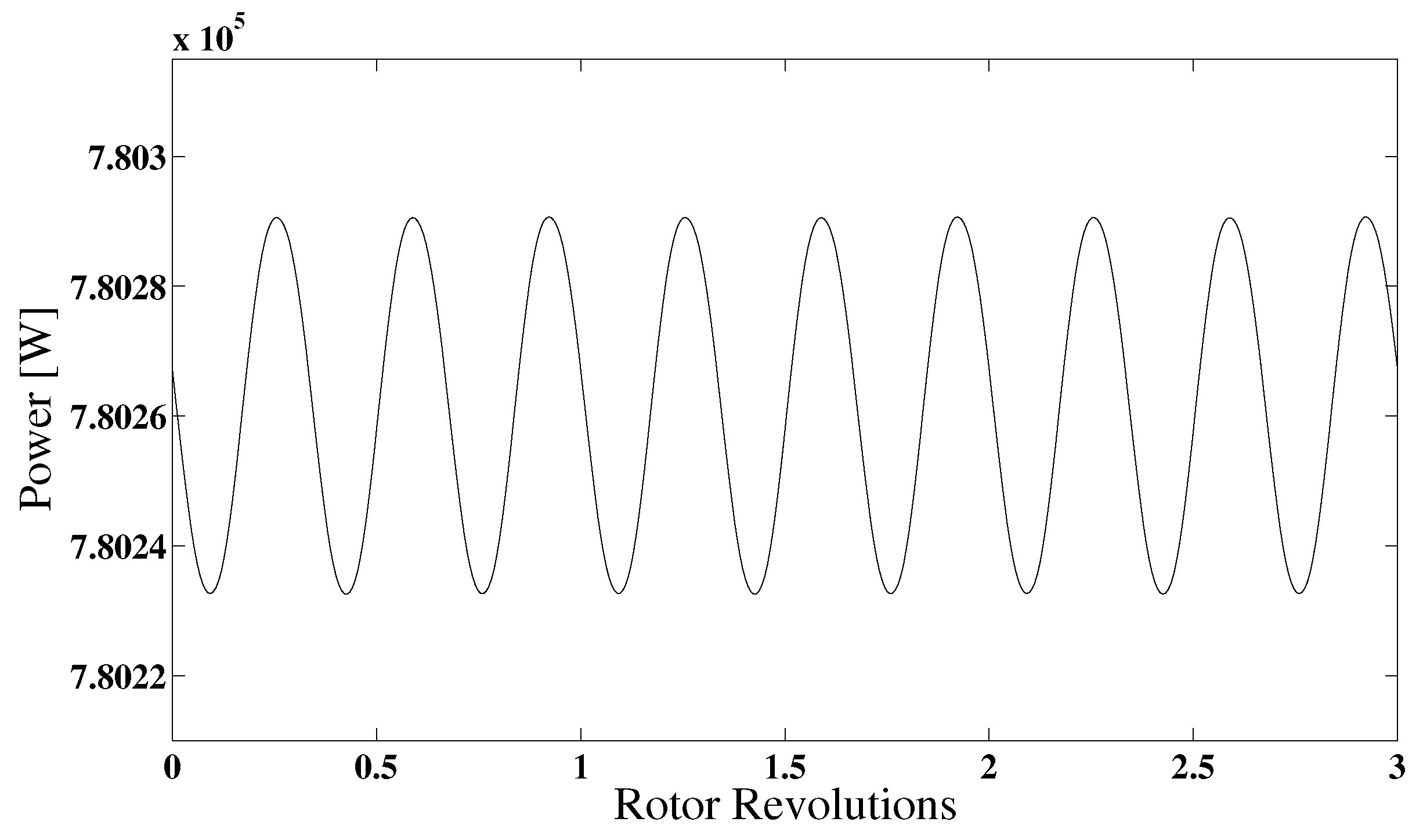
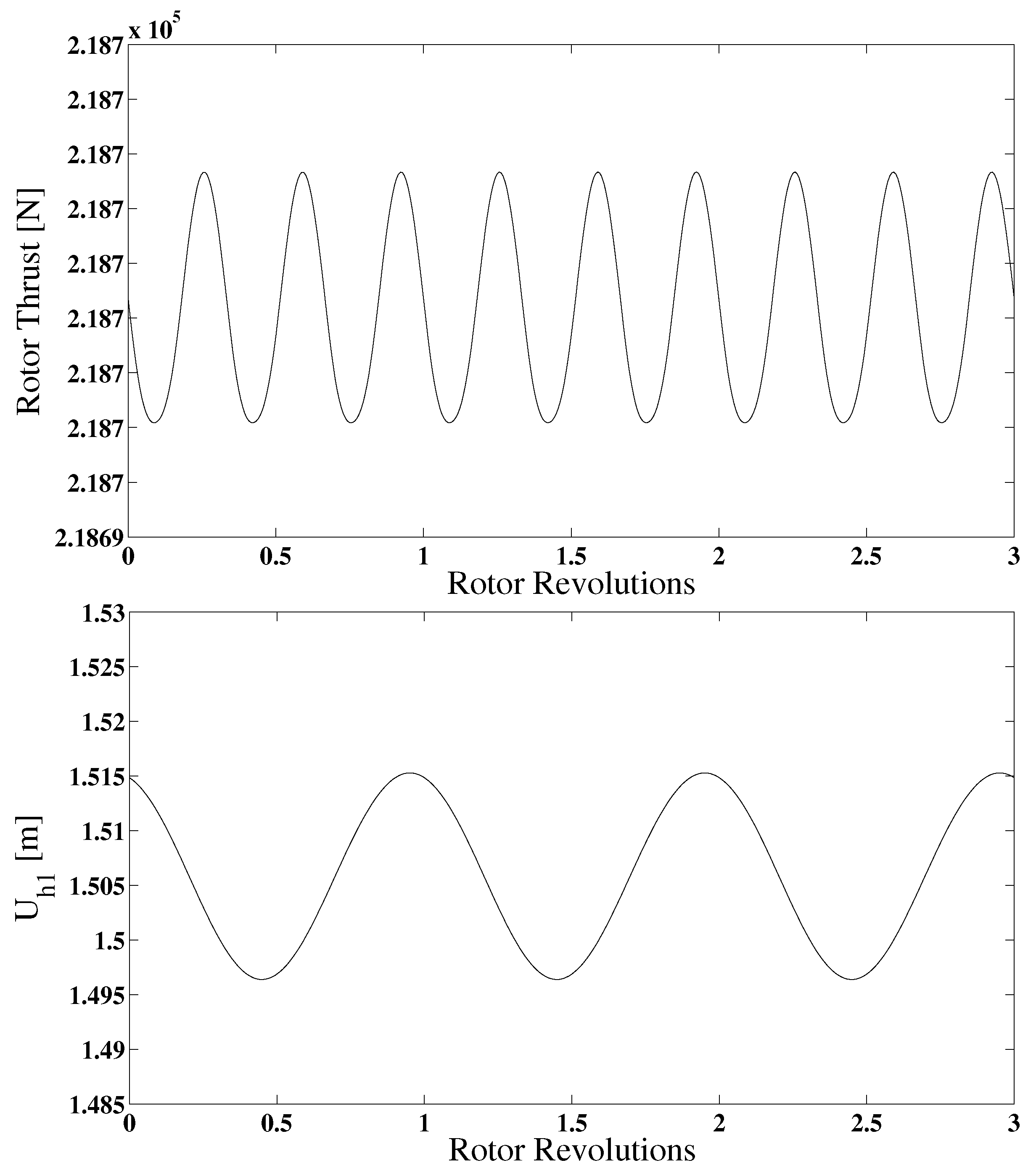
Rotor power, thrust, and displacement of the blade axis, for a section at 90% of the span for an NREL-5MW turbine operating at a typical scenario during its start-up regime, with wind at 6 m/s and rotor speed at 7.9 rpm.
Figure 13.
Rotor power, thrust, and displacement of the blade axis, for a section at 90% of the span for an NREL-5MW turbine operating at a typical scenario during its start-up regime, with wind at 6 m/s and rotor speed at 7.9 rpm.


Figure 14.
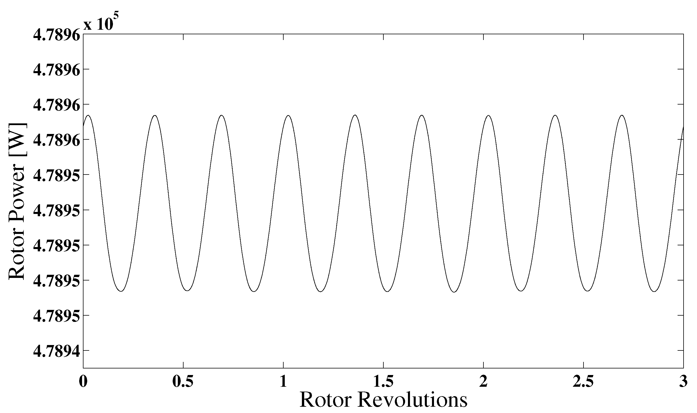
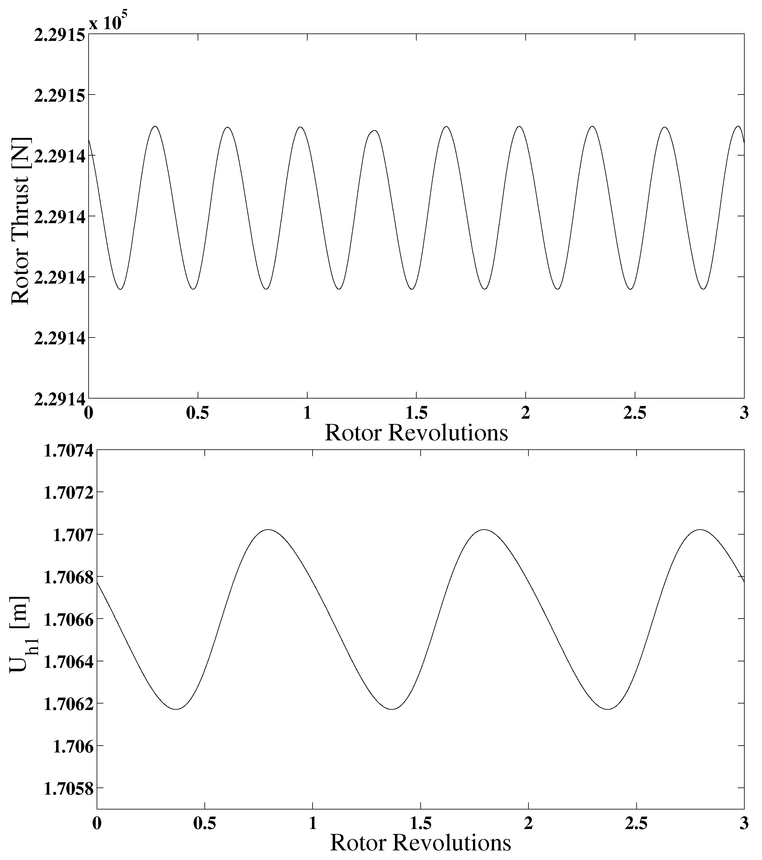
Rotor power, thrust, and displacement of the blade axis, for a section at 90% of the blade span for an NREL-5MW turbine rotating at its nominal speed of 12.1 rpm, with wind suddenly dropping to 5.8 m/s.
Figure 14.
Rotor power, thrust, and displacement of the blade axis, for a section at 90% of the blade span for an NREL-5MW turbine rotating at its nominal speed of 12.1 rpm, with wind suddenly dropping to 5.8 m/s.


© 2019 by the authors. Licensee MDPI, Basel, Switzerland. This article is an open access article distributed under the terms and conditions of the Creative Commons Attribution (CC BY) license (http://creativecommons.org/licenses/by/4.0/).
Share and Cite
MDPI and ACS Style
Rajan, A.; Ponta, F.L. A Novel Correlation Model for Horizontal Axis Wind Turbines Operating at High-Interference Flow Regimes. Energies 2019, 12, 1148. https://doi.org/10.3390/en12061148
AMA Style
Rajan A, Ponta FL. A Novel Correlation Model for Horizontal Axis Wind Turbines Operating at High-Interference Flow Regimes. Energies. 2019; 12(6):1148. https://doi.org/10.3390/en12061148
Chicago/Turabian StyleRajan, Anurag, and Fernando L. Ponta. 2019. "A Novel Correlation Model for Horizontal Axis Wind Turbines Operating at High-Interference Flow Regimes" Energies 12, no. 6: 1148. https://doi.org/10.3390/en12061148
Note that from the first issue of 2016, this journal uses article numbers instead of page numbers. See further details here.