Dynamic Emulation of a PEM Electrolyzer by Time Constant Based Exponential Model


1
Group of Research in Electrical Engineering of Nancy (GREEN), Université de Lorraine/IUT de Longwy, 54401 Longwy, France
2
ICAR, Institute for High Performance Computing and Networking, Italian National Research Council of Italy, 90146 Palermo, Italy
*
Author to whom correspondence should be addressed.
Energies 2019, 12(4), 750; https://doi.org/10.3390/en12040750
Submission received: 24 December 2018
/
Revised: 16 February 2019
/
Accepted: 20 February 2019
/
Published: 24 February 2019
(This article belongs to the Special Issue Selected Papers from EEEIC 2018—18th International Conference on Environment and Electrical Engineering)
Abstract
:The main objective of this paper is to develop a dynamic emulator of a proton exchange membrane (PEM) electrolyzer (EL) through an equivalent electrical model. Experimental investigations have highlighted the capacitive effect of EL when subjecting to dynamic current profiles, which so far has not been reported in the literature. Thanks to a thorough experimental study, the electrical domain of a PEM EL composed of 3 cells has been modeled under dynamic operating conditions. The dynamic emulator is based on an equivalent electrical scheme that takes into consideration the dynamic behavior of the EL in cases of sudden variation in the supply current. The model parameters were identified for a suitable current interval to consider them as constant and then tested with experimental data. The obtained results through the developed dynamic emulator have demonstrated its ability to accurately replicate the dynamic behavior of a PEM EL.
1. Introduction
Over the last years, fossil fuel reserves have significantly decreased due to growing demand. Indeed, fossil fuels are widely used in transportation, industrial and electric power sectors [1]. As a result, intensive use of fossil fuels has had negative impacts and is the main source of air pollution and the primary emitter of carbon dioxide and others greenhouse gas [2,3]. Given that the transportation sector is one the most significant emitters of greenhouse gases, new energy fuel must be developed with the aim to minimize the environmental impact from global warming and meteorological phenomena. Recently, some automotive manufacturers (e.g., Toyota, Honda, and Hyundai) have been interested in hydrogen, with an aim to develop fuel cell electric vehicle prototypes [4,5]. Compared to conventional vehicles that burn fossil fuels, hydrogen combustion only releases water.
At the present time, hydrogen can be manufactured from diverse resources such as fossil fuels, nuclear energy and renewable energy sources (wind, photovoltaic). One of the most attractive and promising solutions for producing hydrogen is water electrolysis based on renewable energy sources. Indeed, water electrolysis a process that uses electricity to split pure water into hydrogen and oxygen. This chemical reaction is carried out by means of an electrolyzer (EL) [6].
Different kind of ELs can be differentiated by their electrolyte and charge carrier: alkaline EL, proton exchange membrane (PEM) EL and solid oxide (SO) EL [7,8]. Currently, Alkaline and PEM technologies are commercially available, whereas solid oxide technology is still in research and development. Alkaline technology is the most mature and widespread compared to PEM technology (still under development). On one hand, this technology has a longer lifetime and lower global cost than PEM ELs. On the other hand, it suffers from having low current density and operating pressure, consequently affecting system volume and hydrogen production costs [7]. In comparison, PEM ELs have several benefits over alkaline ELs, such as high power density and cell efficiency, fast system dynamics, wide partial load range, and high adaptability in terms of operation [7]. However, PEM ELs present several disadvantages in regards to platinum catalysts costs and lifetime. Due to their benefits over alkaline ELs, PEM ELs are an attractive option for integration into power grids, including renewable power generating systems [9,10]. For this reason, a PEM EL has been considered for carrying on this work.
The availability of a model to reproduce the behavior of a real system is crucial to study, as well as to verify how it can be incorporated with its power electronic circuit. As a matter of fact, an EL must be connected to a power converter to be properly supplied, and an equivalent model allows the whole system to be simulated and tested, avoiding the expensive damaging of the PEM EL. The same need occurs with fuel cell systems. The detailed dynamic behavior in which a transient of several seconds is noticeable in the current density is described in [11], where the dynamic response of current density is given by a three-dimensional transient model assessed in [12]. In [13], an electrical circuit to represent the dynamic behavior (employed both for battery and fuel cell) is proposed; this circuit is similar to the one proposed in our paper, but it considers only one time constant. These papers have confirmed their hypotheses, while the present paper aims at obtaining an equivalent circuit of the PEM EL to emulate during hydrogen production. This approach is similar to the one described in [14] that has been carried out for a proton exchange membrane fuel cell (PEMFC); here the model is derived in a suitable current interval to consider its parameters as constants.
Only recently, several PEM EL models have been reported in the literature [15,16,17,18,19,20,21,22,23,24,25,26,27,28,29]. However, the major part of the proposed models is static and does not take into consideration the dynamic behavior of the EL, which is particularly interesting to investigate for power electronics applications. In [22], Yigit and Selamet have proposed a dynamic mathematical model developed in a Matlab Simulink environment.
In [24], Atlam and Kolhe have developed an equivalent electrical model for a PEM EL under steady-state conditions. The static behavior of the EL is modeled by a reversible voltage in series with a resistance related to the different overvoltages (activation, ohmic) during the operation. In [25], Andonov and Antonov have proposed a Simulink implementation of a static model of an EL. By comparison, a dynamic model obtained by using neural networks is reported in [26]; however, this model cannot be exploited by a circuital simulator.
Based on the current state-of-the-art research [15,16,17,18,19,20,21,22,23,24,25,26,27,28,29], this paper analyzes the dynamic behavior of a PEM EL subjected to fast current steps. The main objective here is to develop an equivalent dynamic electrical model. Besides, the novelty of the current paper consists both of a method for the identification of a dynamic circuit equivalent model that considers the contribution of double layer capacitances, and on the design of an emulator intended as a system able to duplicate the operation of equipment using different hardware, unlike computer simulations that require an abstract model of the system to be simulated. On the basis of experimental tests performed on the investigated EL, two-time constants corresponding to different exponentials were identified by a least squares regression (LSR) algorithm. In the developed emulator, the input voltage and current have behaved as in the real PEM EL. In addition, the equivalent circuit has reproduced losses and has allowed the upper limit of hydrogen production to be assessed. Finally, the developed emulator is useful to test the performance of power electronics converters in supplying the EL.
This paper is divided into five sections. After this introduction providing the current state-of-the-art research and motivations for carrying out this work, Section 2 describes the proposed and developed equivalent dynamic electrical model for a PEM EL. Then, in Section 3, the developed experimental test bench is presented and the dynamic behavior of the PEM EL is emphasized. Subsequently, in Section 4, the parameters of the electrical model are determined using a LSR algorithm. Finally, in Section 5, the obtained results from the electrical model and experiments are compared in order to validate the proposed model. Losses, energy efficiency, and hydrogen production are also investigated.
2. Dynamic Circuit Identification
The study is focused on a PEM EL. Currently, hydrogen can be obtained by three different solutions: alkaline, SO and PEM electrolysis cells. Among these, the last is based on a solid polymer electrolyte concept. It offers several advantages such as high current density, which exceeds 2 A/cm2, and the reduction of operational cost and ohmic losses since it requires an electrolyte thinner than the alkaline EL. Moreover, the PEM EL is able to operate with a wide range of power input, thanks to the fast response of the proton transport across the membrane. This last aspect is crucial when the power is supplied by renewable energy sources. Finally, the PEM EL performs an electrochemical compression, delivering hydrogen at high pressure, which makes its storage easier [7].
The total chemical reaction to obtain hydrogen, including the Gibbs energy (237 kJ.mol−1) and the lost energy (48.6 kJ.mol−1), is taken by [7]:
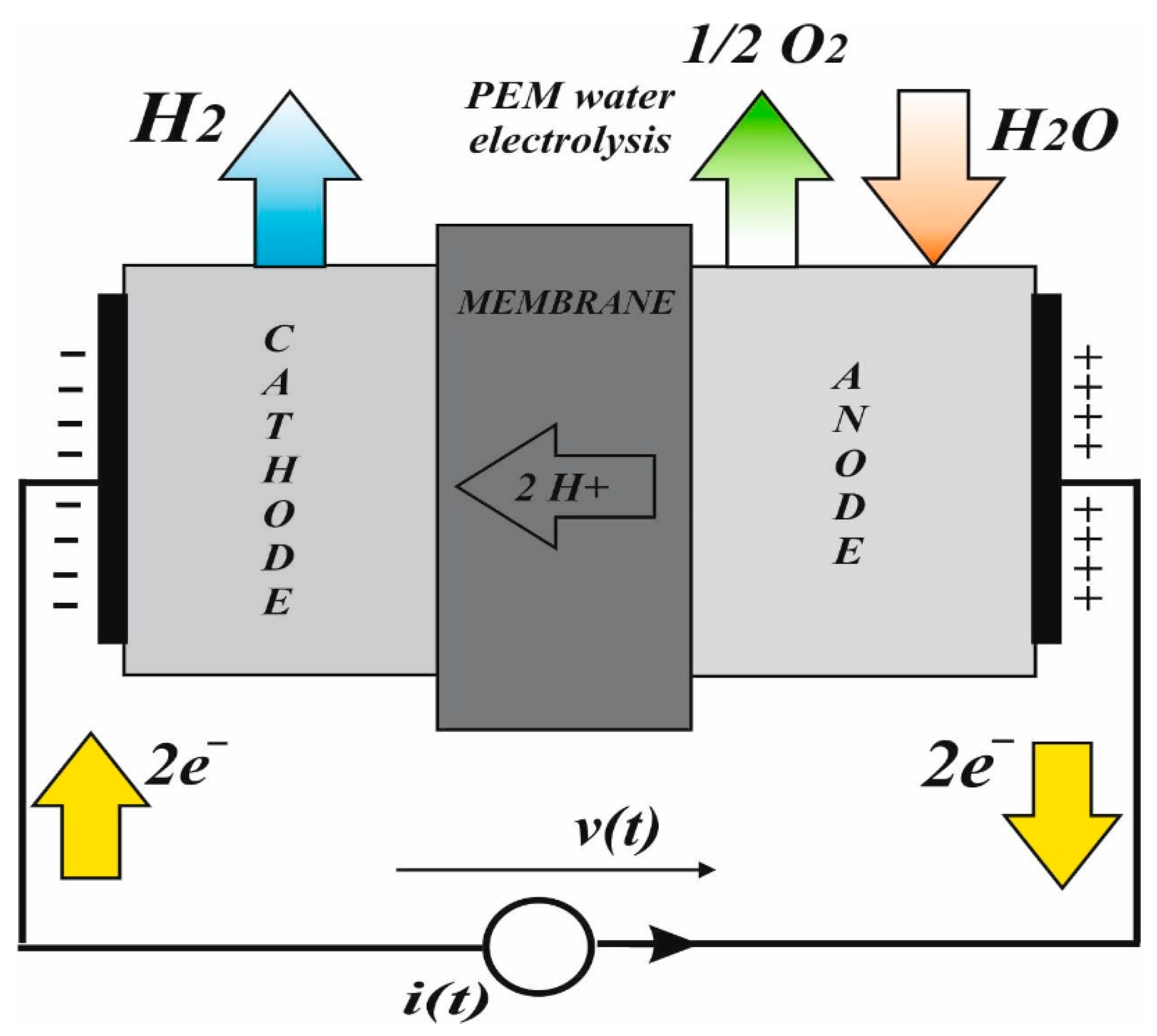
The operation of the PEM EL is shown in Figure 1. It can be noticed that in the anode, connected to a positive electric potential, the water is divided into protons and oxygen, providing electrons for the conduction according to the sub-reaction:
The available electrons go outside the anode and contribute to the current (flowing into the anode), whereas the protons go through the membrane. Once the protons reach the cathode, they combine with electrons coming from the terminal at negative potential, obtaining hydrogen:
The power supplied to the PEM EL cannot be completely converted into high-pressure hydrogen (the PEM EL is able to produce 1 l/h of hydrogen with a pressure of 10 bar) due to the losses. Both the hydrogen production and the losses can be represented by a physical model reproducing the related phenomenon. A resistor is used to emulate losses in the membrane and losses in the two sub-reactions, as well as a voltage generator to produce the hydrogen. In addition, the double layer of charge separation in the anode and in the cathode is obtained by two capacitances. In this way, the dynamic behavior caused by the finite time required by charge layers to vary when a current variation is imposed is reproduced. The two double-layer capacitances can be considered equal following the approach of [14] applied to a PEMFC and validated by measurements. The different speed with which the two sub-reactions (1) and (2) occur with be modelled by different time constants.
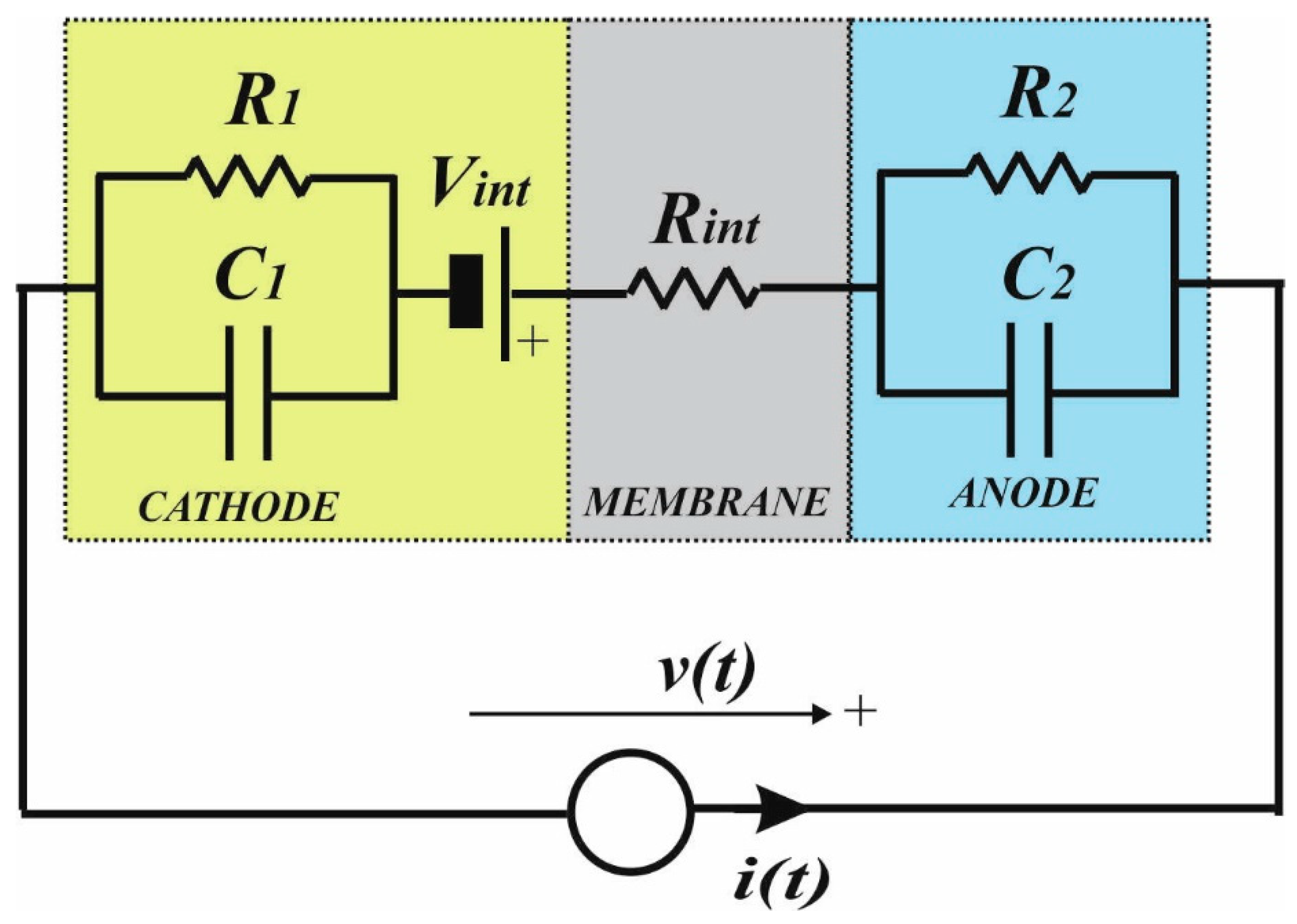
The equivalent circuit model to be identified is shown in Figure 2. The two RC cells represent the behavior in the cathode (R1C1) and in the anode (R2C2) respectively. The Vint voltage reproduces the power converted into hydrogen, whereas the resistance Rint reproduces the losses in the membrane. Contrary to the two capacitances that can be assumed equal, the resistors differ depending on the losses; one resistor models Gibbs energy and the heat loss in the anode, and the other only the heat loss in the cathode.
When a current is supplied to the EL, losses during steady state can be calculated as Joule terms, whereas the power converted into hydrogen is the product of the current by the Vint voltage. When a current transient occurs during a time interval after the variation, the voltage both in the anode and cathode will not vary, and a slight variation will be observed in the voltage at the EL terminals. The voltage will then rise up to the final value after that a new value of the stored charge is restored, depending on the value of the double-layer capacitances.
3. Experimental Test Bench and Investigation of the Dynamic Behavior
3.1. Description of the Experimental Set-Up
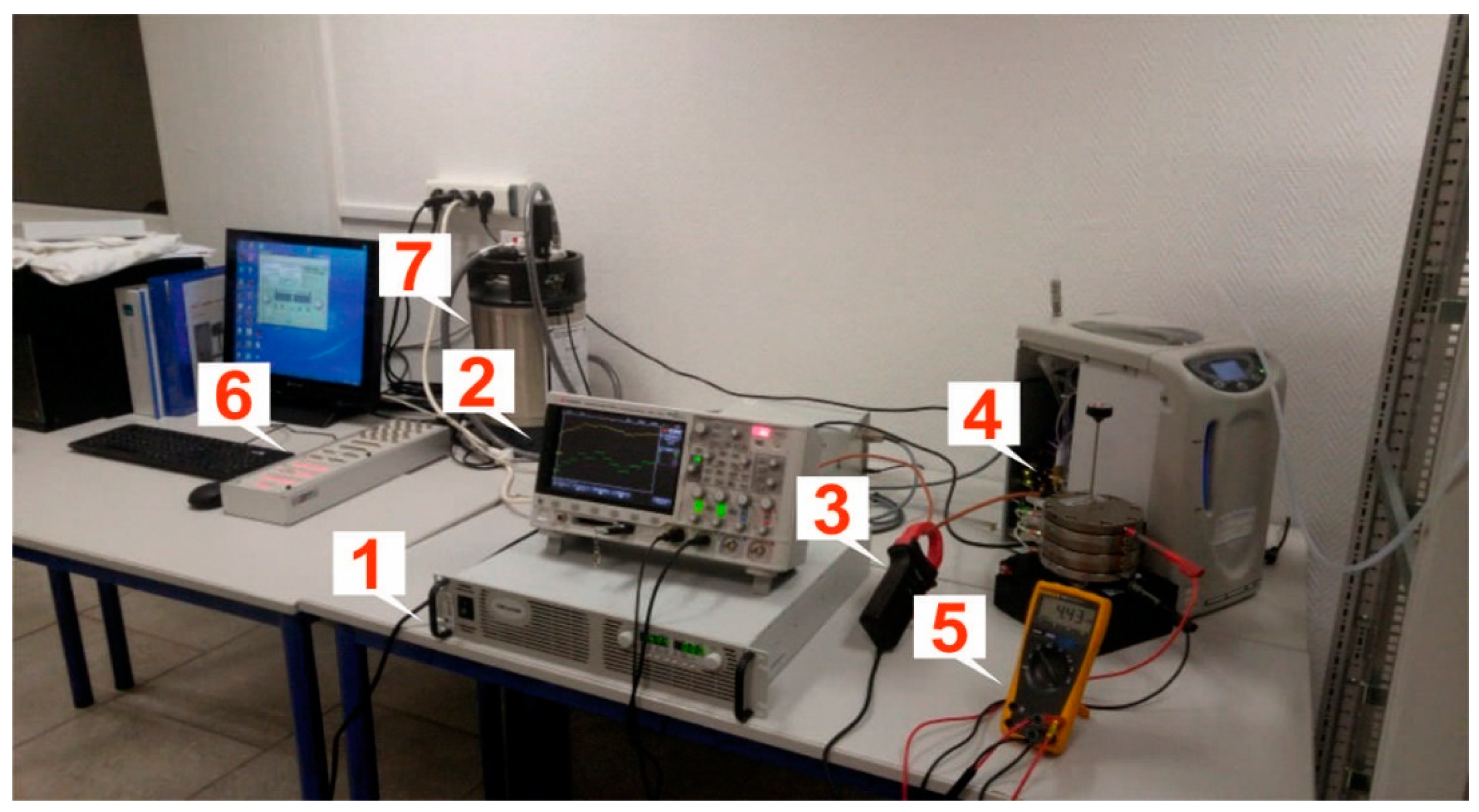
Once the physical model has been assessed, there is need to acquire experimental data to identify the parameters R1, R2, Rint, C1, C2 and Vint. This was done using a suitable test bench. The developed experimental set-up to analyze the dynamic behavior of the PEM EL and to validate the equivalent dynamic electrical model is shown in Figure 3. It is composed of a DC power supply, a PEM EL, low-pressure metal hydride storage hydrogen tanks and a PC to control the DC power supply. Pure water was supplied to the PEM EL by a pure water tank from (SGWATER, Berlin, Germany). The water flow rate was controlled by a liquid mass flow controller from (HELIOCENTRIS, Berlin, Germany). The range included was between 0 and 7.5 L per minute. The water flow rate was controlled automatically according to the operation of the EL.
The PEM EL under investigation is the NMH2 1000 from HELIOCENTRIS (HELIOCENTRIS, Berlin, Germany). Although the HELIOCENTRIS NMH2 1000 system includes several ancillary devices (e.g., power converters), only the stack (and the data acquisition system) has been used in this research. The main characteristics of the PEM EL are provided in Table 1, while the components of the experimental set up are described in Table 2.
During the test, the DC power supply gave a step current to the PEM EL. It was sampled, together with the voltage at the stack terminals, by the digital oscilloscope; data were memorized and elaborated on by the (dSPACE, Bièvres, France) platform to obtain the value of the circuit parameters by the algorithms described in the following section.
3.2. Analysis of the Dynamic Behavior of the PEM EL
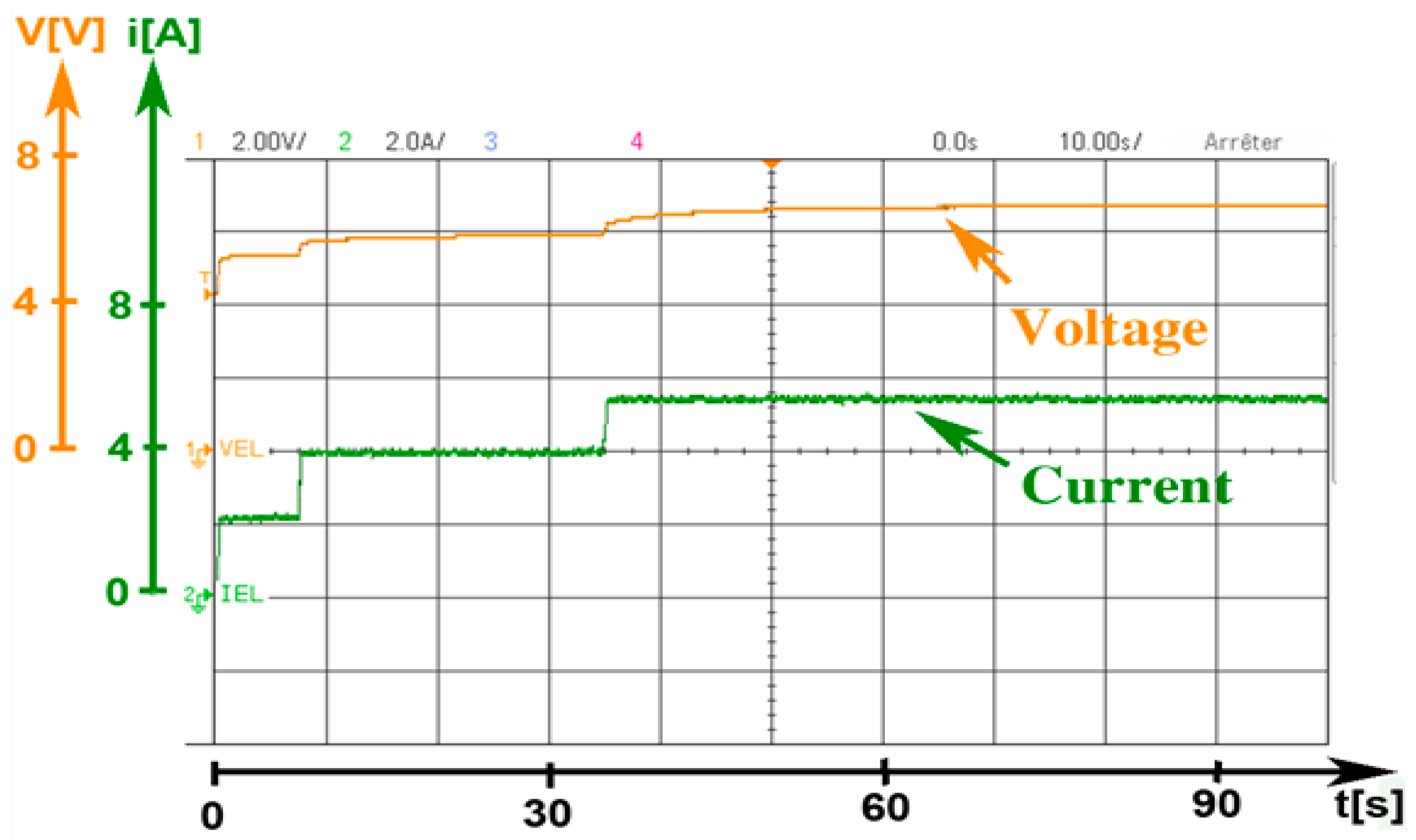
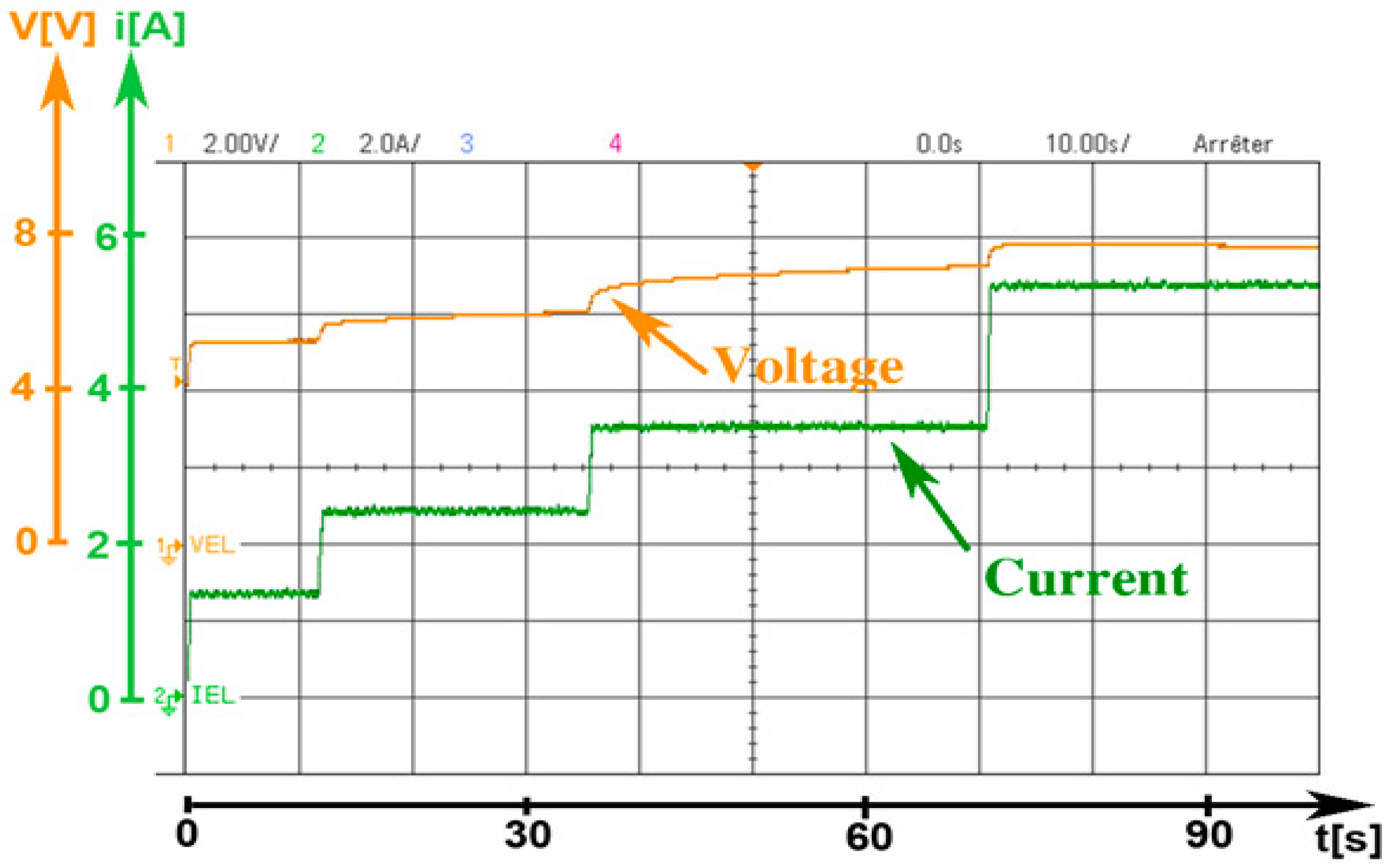
Experimental tests were carried out in order to emphasize the capacitive effect of the PEM EL when subjecting to current steps. The first results obtained are shown in Figure 4 and Figure 5. As can be seen in Figure 4 and Figure 5, the capacitive effect was all the more visible and important for current values greater than 2 A. Indeed, during the first low current step (2 A), the EL voltage reached its permanent value quickly, while for the second variation at 4 A the EL voltage varied very slowly until reaching its value in steady state (≈30 s). For this reason, it can be deduced that precise modeling would require variable circuit parameters, but it is out of the scope of this work which is focused on a method to identify the components of the equivalent circuit. For this reason, identification has been optimized for a suitable current interval adopting constant parameters of the equivalent circuit.
The required time for the stabilization of the PEM EL voltage due to the displacement of the charges inside the anode and the cathode elongated all the more as the current increased. This phenomenon is particularly noticeable in Figure 5. Moreover, this figure clearly shows an operating limit of the PEM EL when the current reaches its maximum threshold (sudden voltage drop). This was an abnormal operation of the PEM EL due to its degradation and was not considered in our model. To conclude, the dynamics of the PEM EL were characterized by two transient phenomena: (1) slowness of the evolution reaction of the oxygen in the anode, and (2) rapidity of the evolution reaction of the hydrogen in the cathode. These two phenomena resulted in the equivalent electrical diagram (Figure 2) by the two RC branches that will be characterized by two different time constants.
4. PEM Electrolyzer Modelling
The equivalent circuit model has been obtained on the basis of experimental testing performed on the PEM EL. Firstly, the static characteristics has been obtained, then the time constants of the dynamic model were identified and calculated by linear regression. Finally, an implementation in a Simulink environment has been performed and the equivalent circuit model has been assessed.
4.1. Experimental Test
Using the experimental set-up described in the previous section, some tests were performed to obtain a database from which information on the dynamic behavior of the EL could be collected. Specifically, the PEM EL was supplied with step current transients.
An example of the voltage and current measured on the EL terminals is shown in Figure 6. In this test, after the power was turned on, the current was increased from 2.34 A to 4 A at t = 20 s; the duration of the test was equal to 100 s waiting for the end of the transient. Different steps of current were considered for supplying the PEM EL.
4.2. Static Model Identification
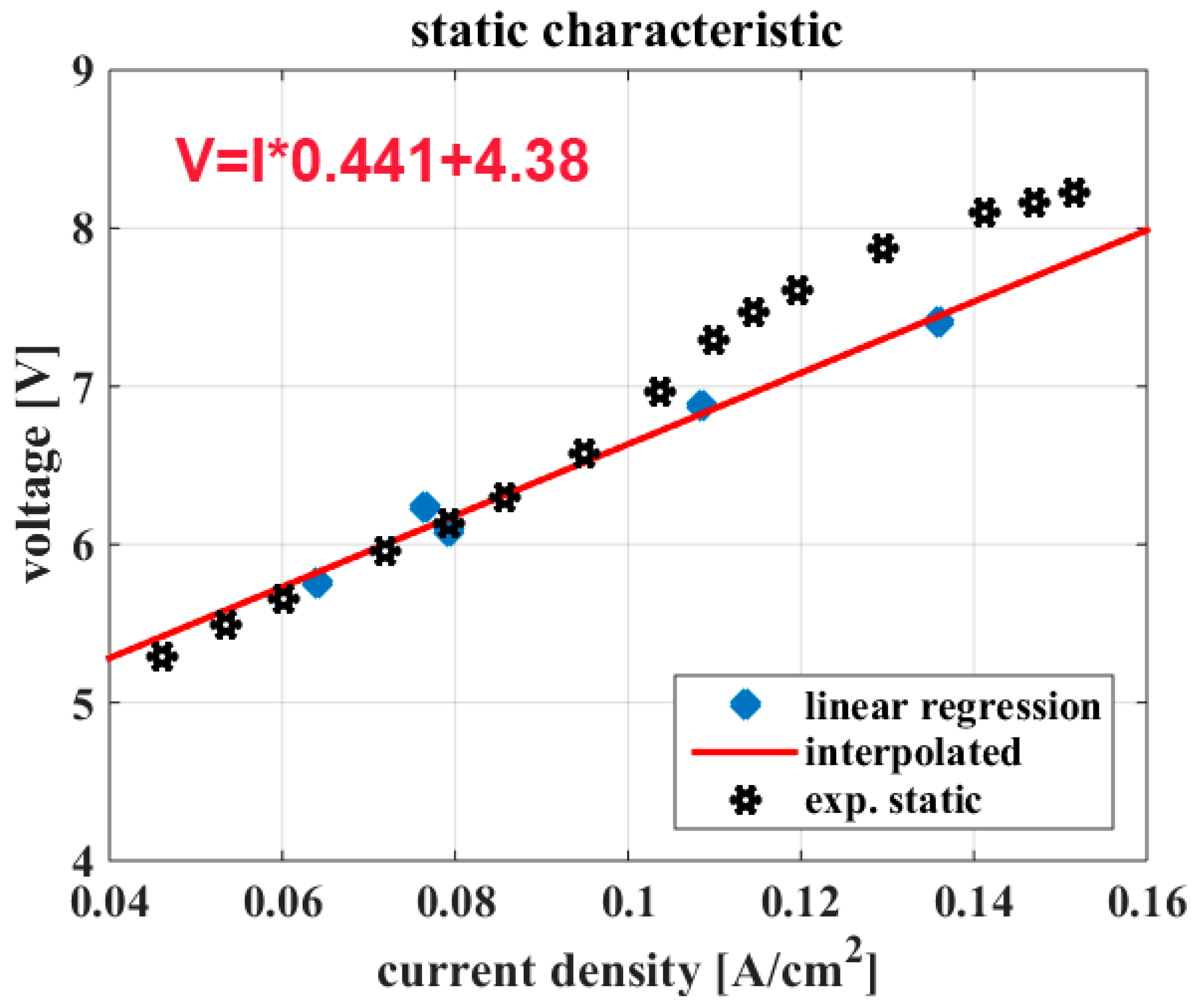
The values of voltage and current measured at the end of each transient were used to identify the static characteristic sketched in Figure 7. These values were calculated at the end of each transient by linear regression when the EL tended to a steady-state operation. It can be noted that the data were sampled in a range from 0.04 A/cm2 to about 0.16 A/cm2, which is of interest for the identification of the model. On the one hand, in this interval, the parameters could be considered as constant. It is an approximation compared with the whole operating range of the EL. Indeed, it can be noted that the more the current is high, the more the error between data acquired by static measurements and those obtained by LSR increases, which was due to the fact that the time required to reach steady-state conditions increased with the current. This confirms that identification with constant parameters is valid in a limited operating range. On the other hand, it is sufficient to assess the methodology that can be applied whatever the selected interval of currents. In the case under study, it represents the operating conditions in which the dynamic model was identified. A least-square regression (LSR) algorithm was used (see Appendix A). From the linear regression on experimental data, the internal resistance was calculated by the slope and the reversible voltage by extrapolating the straight line achieving the electromotive force at zero current. The following values were obtained: Vint = 4.38 V, Rtot = 0.441 Ω. From the waveform of Figure 6, the following considerations can be made: The characteristic resistances Rint can be calculated considering the response after and before the step current and at the end of the transients. Under the hypothesis that the equivalent capacitance is quite high so that immediately after the current is varied the drop voltage occurs only at the Rint terminals, the voltage measured before the step current (at t = 0−) represents the reversible voltage Vint. The internal resistance can be calculated considering the voltage after the current step at t = 0+, it gives:
When all transients are finished, the voltage is proportional to the supply current, and their ratio gives the total equivalent resistance Rtot:
At the end of the transients, the voltage at the PEM EL terminals is given by the product between and the total resistance, giving a constraint to the resistances R1 and R2:
The values of R1 and R2 are calculated on the basis of the time constants identified by the dynamic model supposing that the two equivalent capacitances C1 and C2 are equal. From data shown in Figure 6, the following values have been obtained:
In Figure 7, the equation of the interpolating straight line considering Rtot and Vint by (7) has been included as well. This fits with data obtained by LSR, but the error with static data increases with the current as expected.
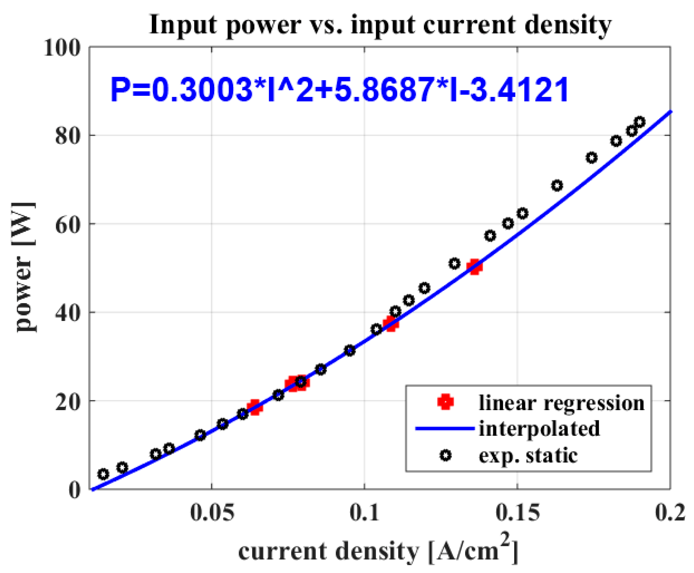
From the static sampled operating point, the input power required by the PEM EL can be calculated as well. This is shown in Figure 8. It can be noted that this relationship is not linear, which can be explained by considering that the losses give a quadratic contribution according to the current. Indeed, this is well approximated by a second-order polynomial curve.
4.3. Dynamic Model Identification
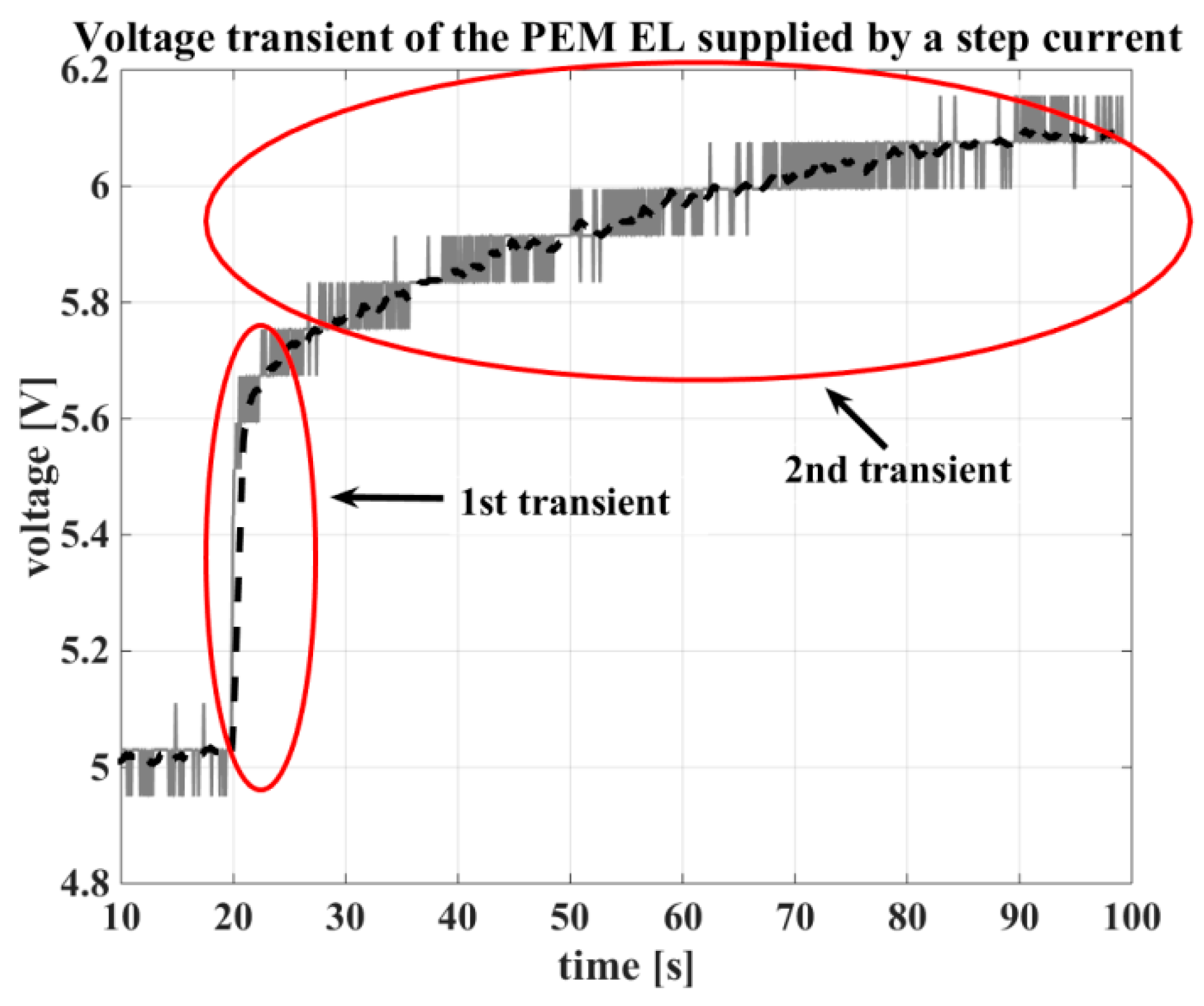
In order to obtain the dynamic model, the transient has been considered considered. It is possible that there were two exponential transients corresponding to two different time constants. This is consistent with the considerations explained in Section 2. The time constants of the dynamic model have been obtained using an LSR algorithm as well (see Appendix A). In this case, since the curves are exponential, some manipulations have been performed in applying the LSR algorithm, as explained in the following.
In the case under study, with a suitable choice of time origin, the voltage profile can be approximated as:
where V0 is the value of the voltage at the instant t = 0+, V∞ is the value of the voltage at the end of the transient (t → ∞) and τ is the time constant of the exponential function. Equation (8) can be rewritten as
With the position
The coefficients to be identified were α and β. The identification was performed both on the exponential curve measured at the beginning of the transient, and on the remaining curve describing the slower transient. The first identification has given the time constants of the anode reaction, and the latter corresponds to the cathode reaction.
In order to minimize noise, filtering was performed by a rolling mean algorithm on 20 samples. A zoom of the two transients together with the filtered data is shown in Figure 9.
The vector of the sampled data contained 2000 samples; to identify the two time constants, the intervals 677–695 and 800–1960 were considered as a trade-off between a suitable number of data to be processed and the exponential curve to be approximated. The values of the time constants obtained were:
Considering the constraints (6) and (11), and assuming that the two capacitances are equal, the following values could be calculated for their equivalent resistances and capacitances:
5. Results
The equivalent circuit shown in Figure 2 has been implemented in a Simulink environment, and the data obtained by the simulation have been compared with the experimental results to validate the model. In the subsequent static test (including efficiency, hydrogen production and temperature assessment of the PEM EL) and dynamic test, the behavior of the PEM EL when soliciting by step currents, has been reproduced are performed. All tests have been performed by acquiring experimental data through the test rig described in Section 3.
5.1. Static Test
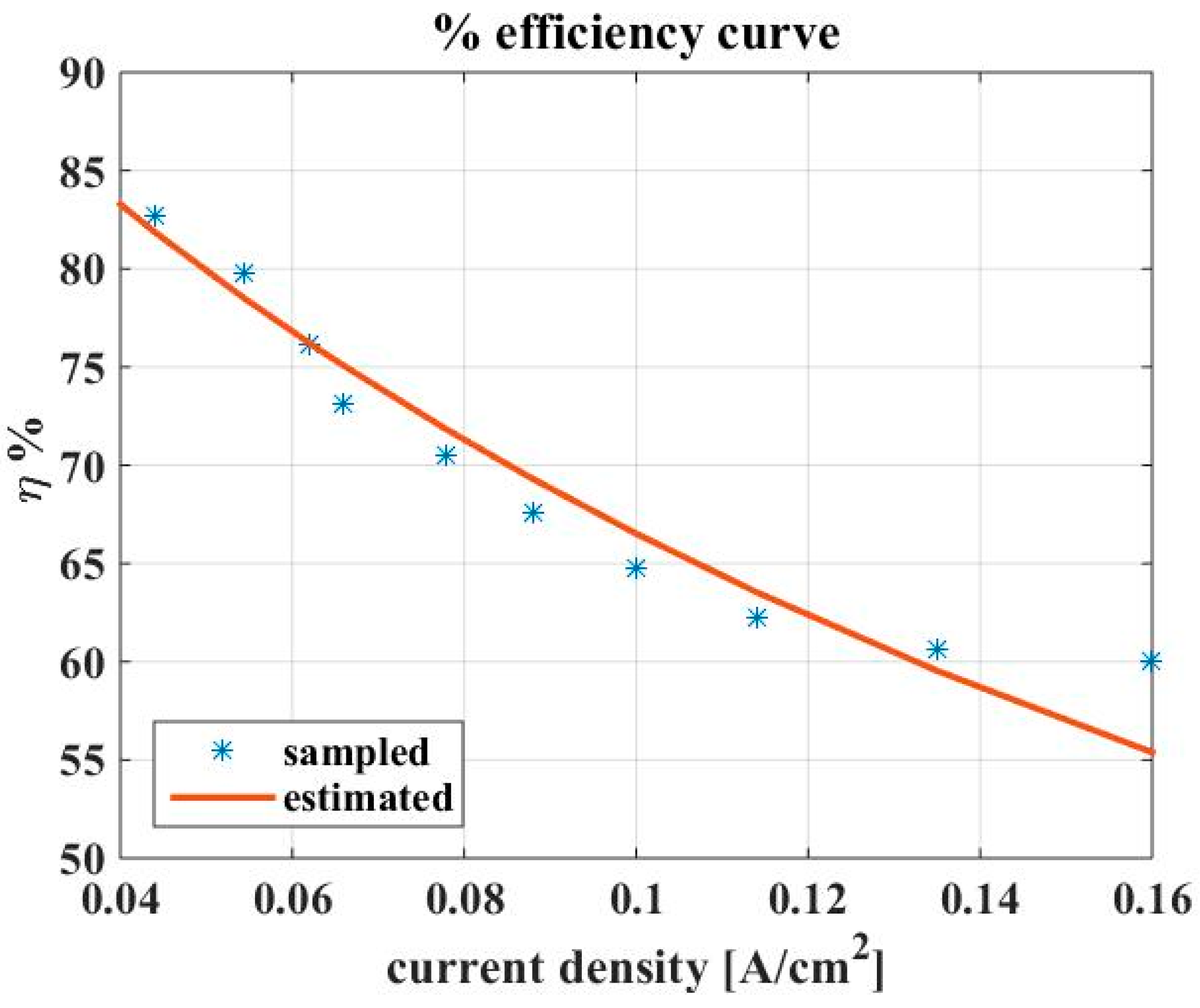
Firstly, the efficiency has been assessed by comparing the estimated data given by the emulator calculated by:
where PH is the power converted into hydrogen and Pin is the electrical power supplied to the PEM EL. The power converted into hydrogen is given by the product between the Vint voltage and the current, whereas the losses have been calculated as the square of the current multiplied for the equivalent resistance into the anode, cathode, and membrane, respectively. It can be noted that the losses are quadratic according to the current, whereas the power converted into hydrogen is linear according to the current. As a result, the overall efficiency decreases according to the current. The efficiency calculated by (13) has been compared with experimental points obtained by the ratio of the produced hydrogen and the power supplied to the PEM EL, where the produced hydrogen is given by substituting the supplied current into the first Faraday’s law of electrolysis to obtain the hydrogen flow rate NH2 [mol/s], then multiplying this value by the higher heating value of the hydrogen (ΔH = 286 kJ/mol). The comparison is shown in Figure 10.
The curves shown in Figure 10 and Figure 11 are influenced by the hypothesis of considering a limited operating range for the identification of a constant parameters model. In particular, each temperature has been obtained at the chosen operating point. For this reason, a polarization curve obtained with constant temperature is not shown. In addition, the calculated production of hydrogen exploits a Faraday’s efficiency value close to one (this is an approximation in the chosen current interval). For this reason, both the efficiency and the hydrogen production rate have to be considered as upper limits.
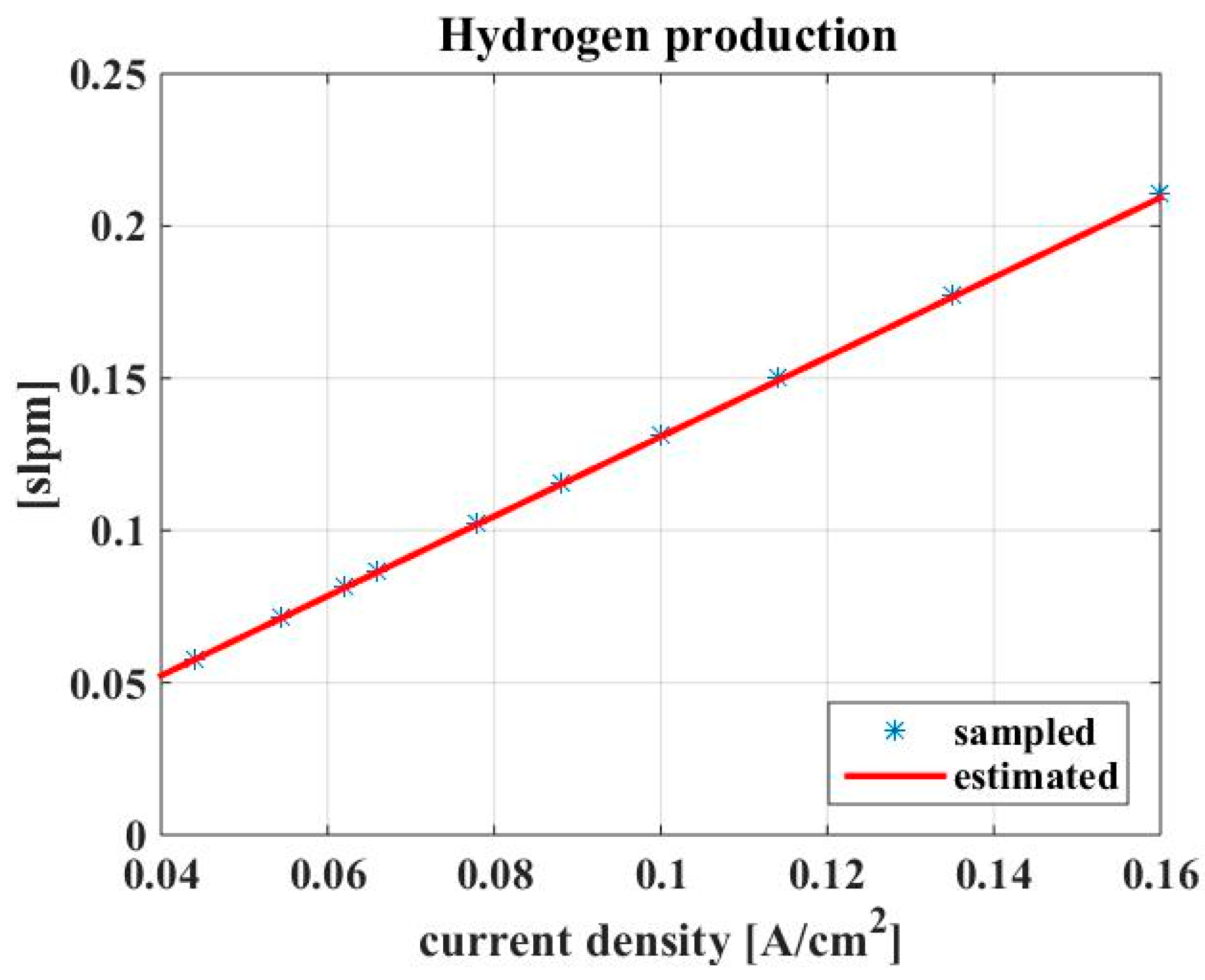
As far as the hydrogen production is concerned, it has been calculated by the emulator on the basis of the product between the internal voltage and the current and compared with experimental points. The produced hydrogen is often given in literature with standard liter per minute (slpm) units defined in standard conditions of T = 288.15 K (i.e., 15 °C) and P = 101.3 kPa. As expected, the produced hydrogen is linear with the current density, and the corresponding curve is shown in Figure 11.
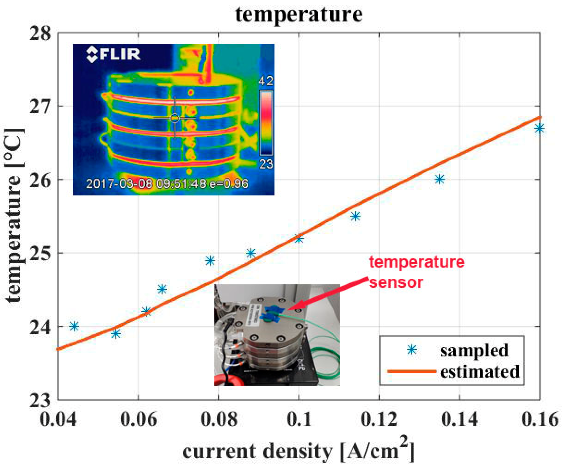
Finally, the measured temperature has been used to calculate the thermal resistance Rth of the PEM EL. It is useful to predict the temperature on the basis of the environmental temperature and on the power supplied to the PEM EL.
The thermal resistance has been obtained by applying the LSR to the quantity:
where Tenv is the environment temperature equal to 23 °C during the test, TEL is the operating temperature of the PEM EL measured after the end of the thermal transient and Pw is the power supplied to the PEM EL. The temperature has been measured by a sensor located on top of the surface and by a thermographic camera as well. However, since the thermographic camera gives a mean temperature of the EL, the curve of Figure 12 is drawn by data coming from the sensor. The temperature has been then estimated by the equation:
Results are shown in Figure 12.
In all the three tests, a good agreement between measured and estimated data is shown.
5.2. Dynamic Test
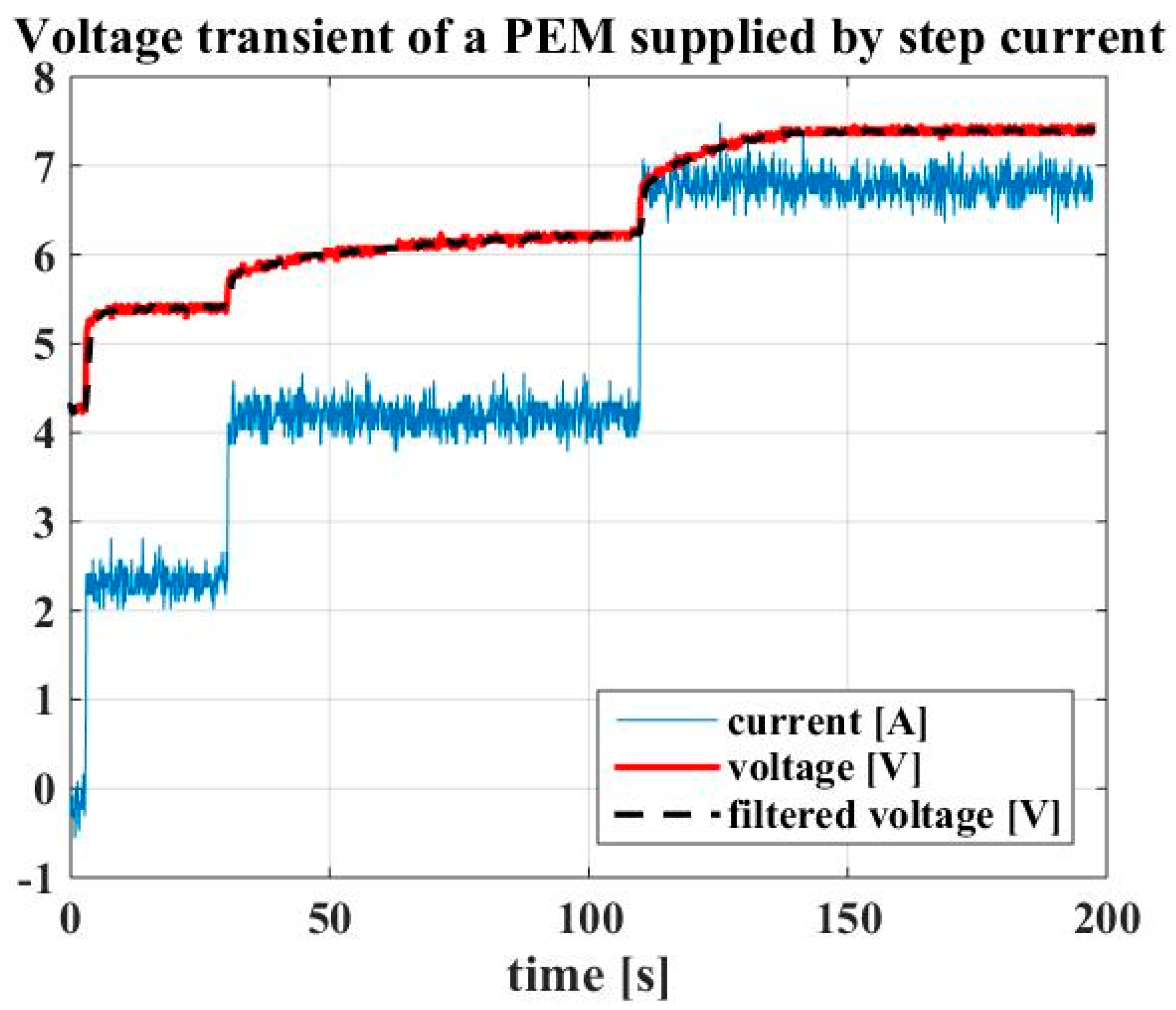
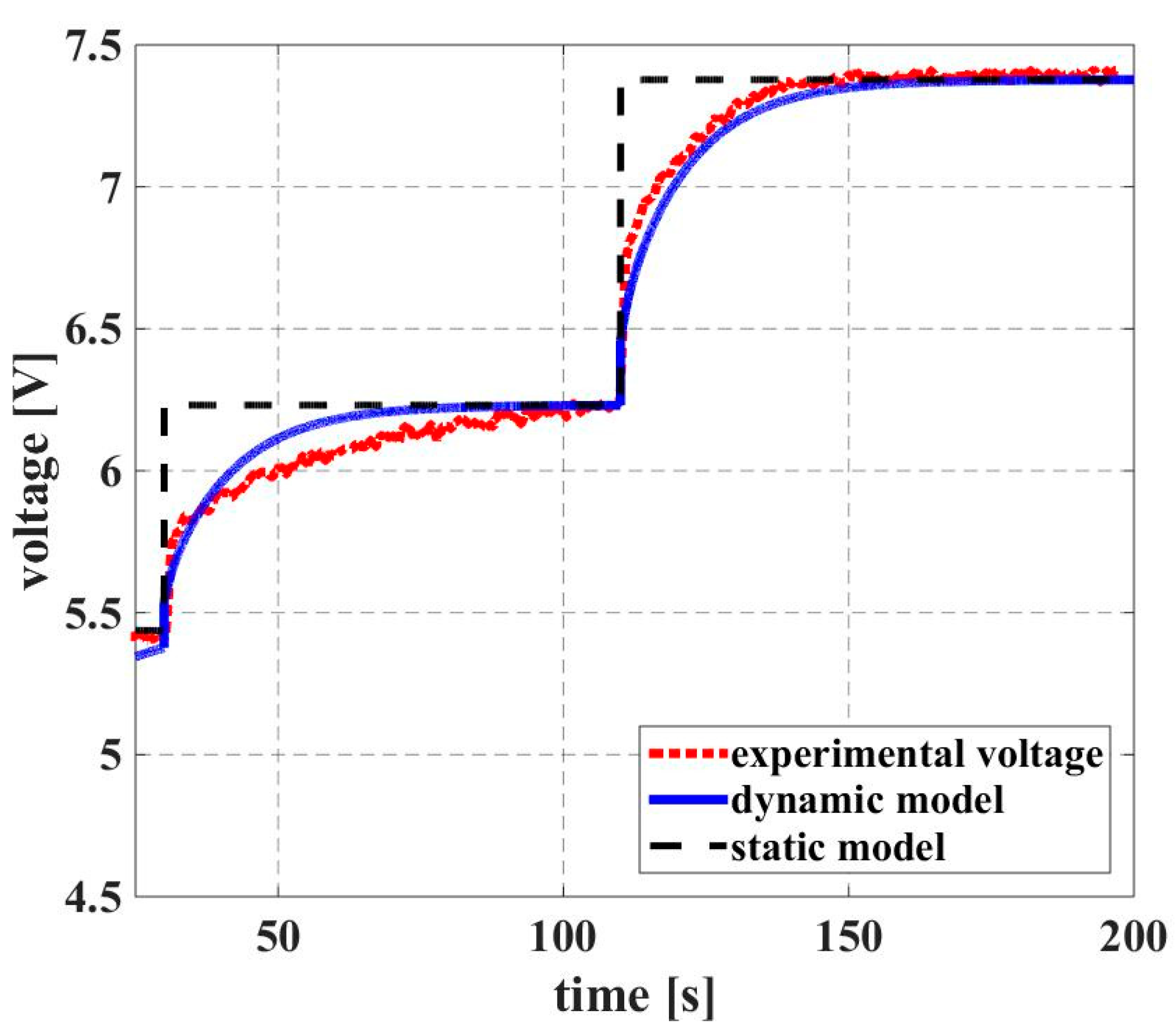
In order to validate the dynamic behavior of the emulator, a transient has been considered in which the supply current went firstly from 5.45 A to 6.25 A at t = 14 s and then to 7.4 A at t = 110 s. The transient has a duration equal to 200 s. In Figure 13, the simulation results have been compared with the experimental data and with the traditional static model without considering the capacitive effects. It can be noted that the curve representing the voltage during transients fits better with experimental data compared to the static model.
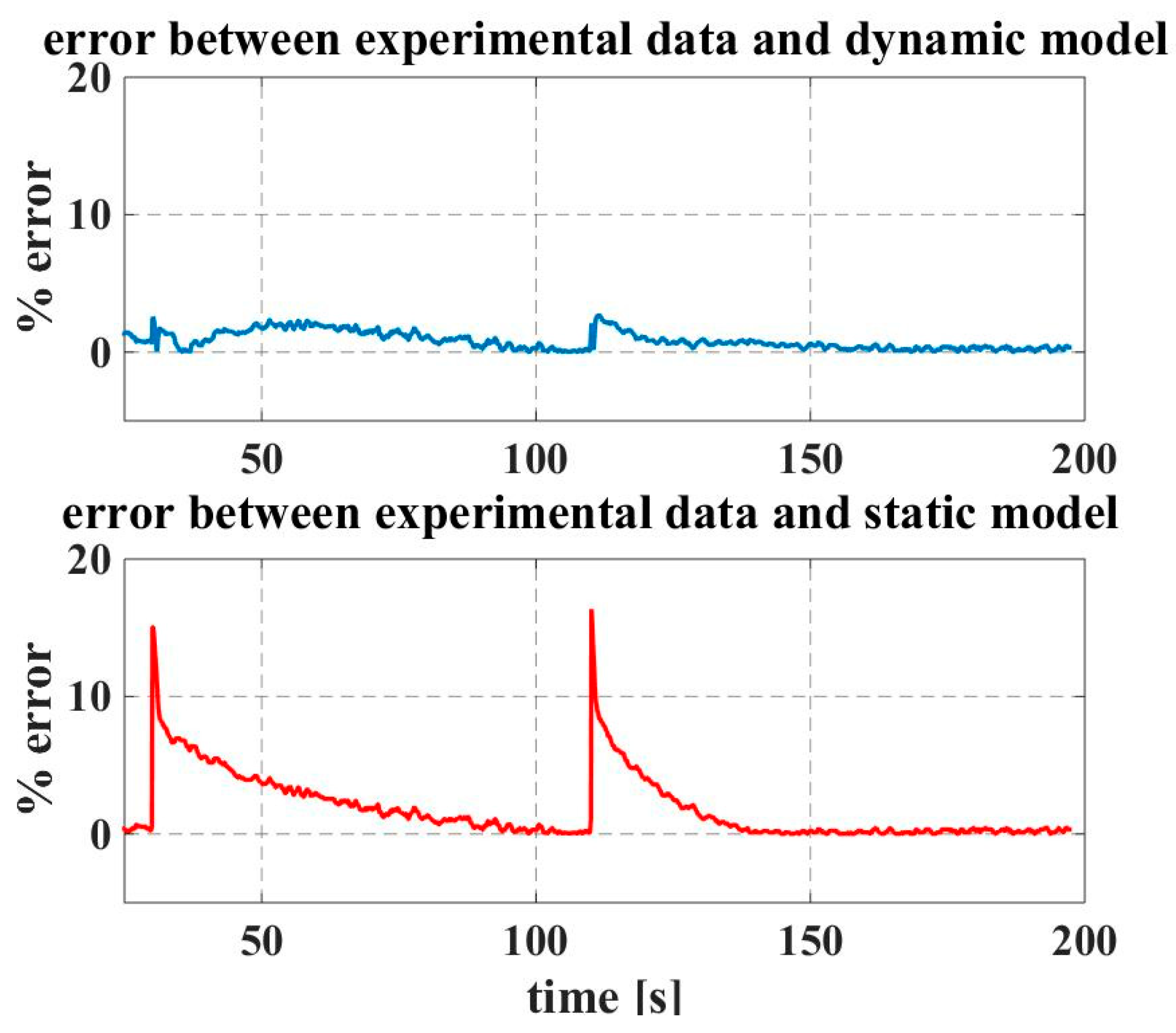
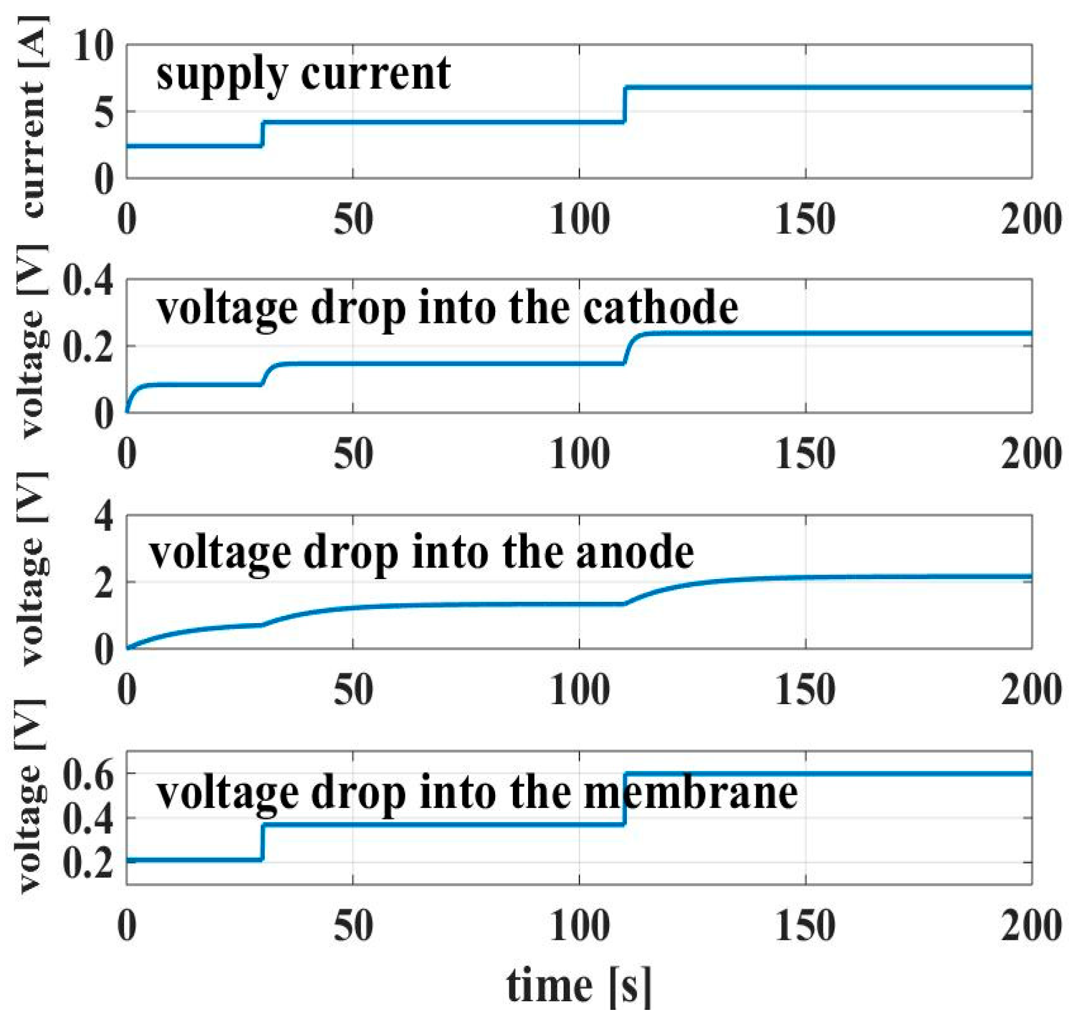
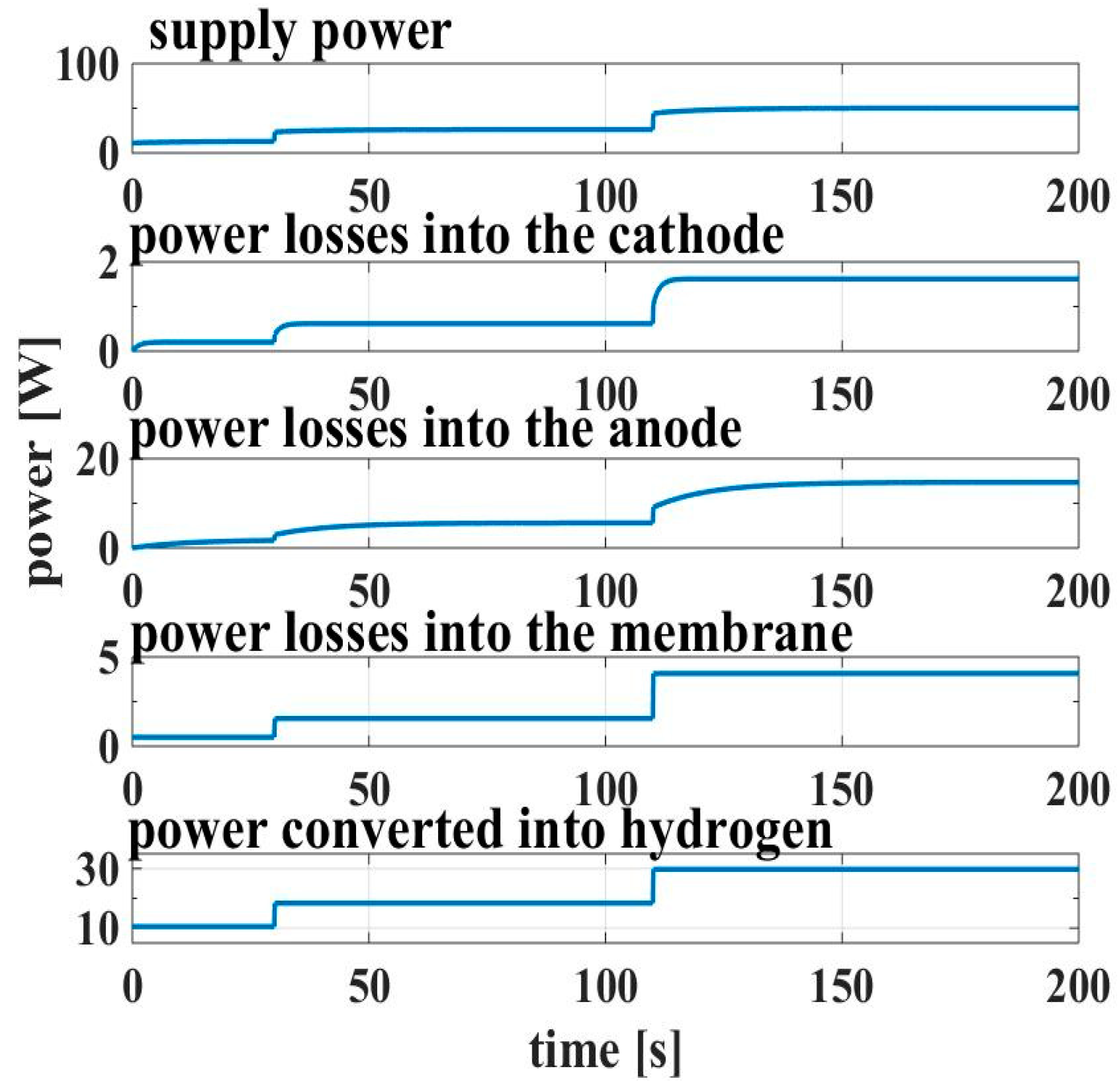
The error between experimental data and the dynamic model (expressed in %) is shown in Figure 14, where it can be noted that the dynamic model shows a maximum error equal to about 4%, whereas the percent error given by the static model increases to 15%. Once validated, the dynamic model, losses and power balance have been calculated during transients. In Figure 15, the voltage drops into the cathode, into the anode and into the membrane are sketched together with the supply current. Figure 16 reproduces the power balance considering the power losses into the cathode, into the anode and into the membrane, as well as the power converted into hydrogen.
It can be noted that by increasing the supply power, all power terms on the PEM EL have increased as expected. In particular, near to the rated current (about 7.4 A in the test), about 50 W have been supplied to the PEM EL and about 30 W have been converted into hydrogen. This is consistent according to the rise of temperature shown in Figure 12.
6. Conclusions
Based on the current state-of-the-art research, the paper aimed at developing an equivalent dynamic electrical model for a PEM electrolyzer. The originality of this work resided in taking into consideration the dynamic behavior of the PEM electrolyzer during sudden variations of the input current. In this specific operating case, the electrolyzer behaves like a capacitor.
The novelty of the paper was to assess the methodology for identifying the exponential time constant equivalent circuit based on a least squares regression algorithm. For this reason, a limited current operating range was chosen to identify a constant parameters model. Even if this interval considered lower current densities compared to the literature, it had the merit of assessing a methodology that can be applied in different current ranges by suitable values of the parameters. Furthermore, this model can be employed to test the behavior of power converters supplying the electrolyzer without risk of damage.
Through experimental results and the use of a least squares regression algorithm, the parameters of the equivalent dynamic electrical model were determined. The comparison between experiments and the obtained results from the developed model demonstrated the accuracy of the model to replicate the real dynamic behavior of an electrolyzer. In addition, the emulator was able to correctly reproduce the temperature, efficiency, and production of hydrogen.
In summary, this electrical model could be useful in exploiting an emulator for experiment purposes, while avoiding the use of an electrolyzer.
Author Contributions
Conceptualization, D.G. and G.V.; methodology, D.G. and G.V.; validation, D.G. and G.V.; investigation, D.G. and G.V.; writing—original draft preparation, D.G. and G.V.; writing—review and editing, D.G. and G.V.
Funding
This research received no external funding.
Acknowledgments
The authors would like to thank the technical staff at the IUT of Longwy, Serge Merafina, for his valuable advices regarding the development and realization of the experimental test bench.
Conflicts of Interest
The authors declare no conflict of interest.
Appendix A
The LSR algorithm minimizes the Euclidean distance between the points yi and f(xi) given by:
If the function to be identified is linear in respect to m parameters pk (where the number of the parameters m is supposed much lower than the measurements n), it can be written as:
The following linear system can be defined:
where:
The minimization of the quantity S is obtained by minimizing the norm of the residual:
It corresponds to impose that the derivative of the square of the norm with respect to the coefficients pk is equal to zero:
Rewriting (A6) in matrix form:
If the rank of A is complete, ATA can be inverted and the vector p is given by:
In this work, the LSR algorithm has been applied to identify the static characteristic, which is linear as shown in Figure 5, and the time constants of the transients of a dynamic model. In this case, the exponential curve has been multiplied by an algorithm to obtain a linear function in which the slope is the time constant.
References
- Mutarraf, M.U.; Terriche, Y.; Niazi, K.A.K.; Vasquez, J.C.; Guerrero, J.M. Energy Storage Systems for Shipboard Microgrids—A Review. Energies 2018, 11, 3492. [Google Scholar] [CrossRef]
- Mumtaz, S.; Ali, S.; Ahmad, S.; Khan, L.; Hassan, S.Z.; Kamal, T. Energy Management and Control of Plug-In Hybrid Electric Vehicle Charging Stations in a Grid-Connected Hybrid Power System. Energies 2017, 10, 1923. [Google Scholar] [CrossRef]
- Mostert, C.; Ostrander, B.; Bringezu, S.; Kneiske, T.M. Comparing Electrical Energy Storage Technologies Regarding Their Material and Carbon Footprint. Energies 2018, 11, 3386. [Google Scholar] [CrossRef]
- Tanç, B.; Arat, H.T.; Baltacıoğlu, E.; Aydın, k. Overview of the next quarter century vision of hydrogen fuel cell electric vehicles. Int. J. Hydrogen Energy 2018. [Google Scholar] [CrossRef]
- Li, H.; Ravey, A.; N’Diaye, A.; Djerdir, A. A Review of Energy Management Strategy for Fuel Cell Hybrid Electric Vehicle. In Proceedings of the 2017 IEEE Vehicle Power and Propulsion Conference (VPPC), Belfort, France, 11–14 December 2017; pp. 1–6. [Google Scholar]
- Mohanpurkar, M.; Luo, Y.; Terlip, D.; Dias, F.; Harrison, K.; Eichman, J.; Hovsapian, R.; Kurtz, J. Electrolyzers Enhancing Flexibility in Electric Grids. Energies 2017, 10, 1836. [Google Scholar] [CrossRef]
- Carmo, M.; Fritz, D.L.; Mergel, J.; Stolten, D. A comprehensive review on PEM water electrolysis. Int. J. Hydrogen Energy 2013, 38, 4901–4934. [Google Scholar] [CrossRef]
- Koponen, J. Review of Water Electrolysis Technologies and Design of Renewable Hydrogen Production Systems. Master’s Thesis, Lappeen University of Technology, Lappeenranta, Finland, 2015. [Google Scholar]
- Gracia, L.; Casero, P.; Bourasseau, C.; Chabert, A. Use of Hydrogen in Off-Grid Locations, a Techno-Economic Assessment. Energies 2018, 11, 3141. [Google Scholar] [CrossRef]
- Kharel, S.; Shabani, B. Hydrogen as a Long-Term Large-Scale Energy Storage Solution to Support Renewables. Energies 2018, 11, 2825. [Google Scholar] [CrossRef]
- Wang, Y.; Wang, C.Y. Transient analysis of polymer electrolyte fuel cells. Electrochim. Acta 2005, 50, 1307–1315. [Google Scholar] [CrossRef]
- Wang, Y.; Wang, C.Y. Two-phase transients of polymer electrolyte fuel cells. J. Electrochem. Soc. 2007, 154, B636–B643. [Google Scholar] [CrossRef]
- Amphlett, J.C.; de Oliveira, E.H.; Mann, R.F.; Roberge, P.R.; Rodrigues, A.; Salvador, J.P. Dynamic interaction of a proton exchange membrane fuel cell and a lead-acid battery. J. Power Sources 1997, 65, 173–178. [Google Scholar] [CrossRef]
- Hinaje, M.; Raël, S.; Noiying, P.; Nguyen, D.A.; Davat, B. An Equivalent Electrical Circuit Model of Proton Exchange Membrane Fuel Cells Based on Mathematical Modelling. Energies 2012, 5, 2724–2744. [Google Scholar] [CrossRef] [Green Version]
- Ruuskanen, V.; Koponen, J.; Huoman, K.; Kosonen, A.; Niemela, M.; Ahola, J. PEM water electrolyzer model for a power-hardware-in-loop simulator. Int. J. Hydrogen Energy 2017, 42, 10775–10784. [Google Scholar] [CrossRef]
- Sarrias-Mena, R.; Fernandez-Ramirez, L.M.; Garcia-Vasquez, C.A.; Jurado, F. Electrolyzer models for hydrogen production from wind energy systems. Int. J. Hydrogen Energy 2015, 40, 2927–2938. [Google Scholar] [CrossRef]
- Awasthi, A.; Scott, K.; Basu, S. Electrolyzer models for hydrogen production from wind energy systems. Int. J. Hydrogen Energy 2011, 36, 14779–14786. [Google Scholar] [CrossRef]
- Han, B.; Steen III, S.M.; Mo, J.; Zhang, F.Y. Electrochemical performance modeling of a proton exchange membrane electrolyzer cell for hydrogen energy. Int. J. Hydrogen Energy 2015, 40, 7006–7016. [Google Scholar] [CrossRef] [Green Version]
- Han, B.; Steen, S.M., III; Mo, J.; Zhang, F.Y. Modelling and simulation of a proton exchange membrane (PEM) electrolyser cell. Int. J. Hydrogen Energy 2015, 40, 13243–13257. [Google Scholar] [CrossRef]
- Abdol Rahim, A.H.; Tijani, A.S.; Kamarudin, S.K.; Hanapi, S. An overview of polymer electrolyte membrane electrolyzer for hydrogen production: Modeling and mass transport. J. Power Sources 2016, 309, 56–65. [Google Scholar] [CrossRef]
- Espinosa-Lopez, M.; Darras, C.; Poggi, P.; Glises, R.; Baucour, P.; Rakotondrainibe, A.; Besse, S.; Serre-Combe, P. Modelling and experimental validation of a 46 kW PEM high pressure water electrolyzer. Renew. Energy 2018, 119, 160–173. [Google Scholar] [CrossRef]
- Yigit, T.; Faruk Selamet, O. Mathematical modeling and dynamic simulink simulation of high-pressure PEM electrolyzer system. Int. J. Hydrogen Energy 2016, 41, 13901–13914. [Google Scholar] [CrossRef]
- Aouali, F.Z.; Becherif, M.; Ramadan, H.S.; Emziane, M.; Khellaf, A.; Mohammedi, K. Analytical modelling and experimental validation of proton exchange membrane electrolyser for hydrogen production. Int. J. Hydrogen Energy 2017, 42, 1366–1374. [Google Scholar] [CrossRef]
- Atlam, O.; Kolhe, M. Equivalent electrical model for a proton exchange membrane (PEM) electrolyser. Energy Convers. Manag. 2011, 52, 2952–2957. [Google Scholar] [CrossRef]
- Andonov, A.; Antonov, L. Modeling of an electrolyzer for а hybrid power supply system. Sci. Eng. Educ. 2016, 1, 36–38. [Google Scholar]
- Belmokhtar, K.; Doumbia, M.L.; Agbossou, K. Dynamic Model of an Alkaline Electrolyzer Based an Artificial Neural Networks. In Proceedings of the Eighth International Conference and Exhibition on Ecological Vehicles and Renewable Energies (EVER), Monte Carlo, Monaco, 27–30 March 2013; pp. 1–4. [Google Scholar]
- Liso, V.; Savoia, G.; Araya, S.S.; Cinti, G.; Kær, S.K. Modelling and Experimental Analysis of a Polymer Electrolyte Membrane Water Electrolysis Cell at Different Operating Temperatures. Energies 2018, 11, 3273. [Google Scholar] [CrossRef]
- Sánchez, M.; Amores, E.; Rodríguez, L.; Clemente-Jul, C. Semi-empirical model and experimental validation for the performance evaluation of a 15 kW alkaline water electrolyzer. Int. J. Hydrogen Energy 2018, 43, 20332–20345. [Google Scholar] [CrossRef]
- Corengia, M.; Torres, A.I. Two-phase Dynamic Model for PEM Electrolyzer. Comput. Aided Chem. Eng. 2018, 44, 1435–1440. [Google Scholar]
Figure 1.
Proton exchange membrane (PEM) water electrolysis reactions. In the anode, the water is divided into protons and oxygen providing electrons; in the cathode, the protons combine with electrons coming from the terminal at negative potential, obtaining hydrogen.
Figure 1.
Proton exchange membrane (PEM) water electrolysis reactions. In the anode, the water is divided into protons and oxygen providing electrons; in the cathode, the protons combine with electrons coming from the terminal at negative potential, obtaining hydrogen.

Figure 2.
Equivalent electric scheme of the PEM electrolyzer (EL).

Figure 3.
Developed experimental set up with the PEM EL: (1) DC power supply, (2) digital oscilloscope, (3) current clamp, (4) PEM EL stack, (5) digital multimeter, (6) dSPACE board, (7) pressurized pure water tank.
Figure 3.
Developed experimental set up with the PEM EL: (1) DC power supply, (2) digital oscilloscope, (3) current clamp, (4) PEM EL stack, (5) digital multimeter, (6) dSPACE board, (7) pressurized pure water tank.

Figure 4.
Demonstration of the capacitive effect of the EL. Channel 1: EL voltage (2 V.div−1), channel 2: EL current (2 A.div−1), time: 10 s.div−1.
Figure 4.
Demonstration of the capacitive effect of the EL. Channel 1: EL voltage (2 V.div−1), channel 2: EL current (2 A.div−1), time: 10 s.div−1.

Figure 5.
Operating limits of the PEM EL. Channel 1: EL voltage (2 V.div−1), channel 2: EL current (2 A.div−1), time: 10 s.div−1.
Figure 5.
Operating limits of the PEM EL. Channel 1: EL voltage (2 V.div−1), channel 2: EL current (2 A.div−1), time: 10 s.div−1.

Figure 6.
Example of voltage transient.

Figure 7.
Static characteristic obtained by linear regression and experimental measurements.

Figure 8.
Input power vs. the current density supplied to the PEM EL.

Figure 9.
Zoom of the transient with exponential curves.

Figure 10.
Upper limit of the efficiency for the PEM EL.

Figure 11.
Upper limit of the of hydrogen production vs. current density.

Figure 12.
Experimental and estimated temperature of the PEM EL.

Figure 13.
Comparison among the PEM EL voltage: experimental, obtained by dynamic model and by static model.
Figure 13.
Comparison among the PEM EL voltage: experimental, obtained by dynamic model and by static model.

Figure 14.
Error percentage obtained comparing the experimental data with the dynamic model (top) and the static model (bottom).
Figure 14.
Error percentage obtained comparing the experimental data with the dynamic model (top) and the static model (bottom).

Figure 15.
Voltage drop into the cathode, into the anode and into the membrane together with the supply current.
Figure 15.
Voltage drop into the cathode, into the anode and into the membrane together with the supply current.

Figure 16.
Power balance of the PEM EL.


Table 1.
Main features of the investigated PEM EL.
| Parameters | Value | Unit |
|---|---|---|
| Rated electrical power | 400 | W |
| Stack operating voltage range | 7.5–8 | V |
| Stack current range | 0–50 | A |
| Delivery output pressure | 0.1–10.5 | bar |
| Cells number | 3 | - |
| Active area Section | 50 | cm2 |
Table 2.
Components of the measurement system.
| Component | Producer | Model |
|---|---|---|
| DC Power Supply | TDK | GEN60-55 |
| Pure water tank | SGWATER | SG 2000 |
| Digital Oscilloscope | Tektronix | MDO3054 |
| Current clamp | Chauvin Arnoux | PAC10 |
| PEM EL | HELIOCENTRIS | NMH2 1000 |
| Digital multimeter | Fluke | 179 |
| dSPACE board | dSPACE | DS1104 |
| Hydrogen tank | HELIOCENTRIS | 760 NI |
© 2019 by the authors. Licensee MDPI, Basel, Switzerland. This article is an open access article distributed under the terms and conditions of the Creative Commons Attribution (CC BY) license (http://creativecommons.org/licenses/by/4.0/).
Share and Cite
MDPI and ACS Style
Guilbert, D.; Vitale, G. Dynamic Emulation of a PEM Electrolyzer by Time Constant Based Exponential Model. Energies 2019, 12, 750. https://doi.org/10.3390/en12040750
AMA Style
Guilbert D, Vitale G. Dynamic Emulation of a PEM Electrolyzer by Time Constant Based Exponential Model. Energies. 2019; 12(4):750. https://doi.org/10.3390/en12040750
Chicago/Turabian StyleGuilbert, Damien, and Gianpaolo Vitale. 2019. "Dynamic Emulation of a PEM Electrolyzer by Time Constant Based Exponential Model" Energies 12, no. 4: 750. https://doi.org/10.3390/en12040750
Note that from the first issue of 2016, this journal uses article numbers instead of page numbers. See further details here.