Performant and Simple Numerical Modeling of District Heating Pipes with Heat Accumulation


Energy Institute, Faculty of Mechanical Engineering, Brno University of Technology—VUT Brno, Technicka 2896/2, 61669 Brno, Czech Republic
*
Author to whom correspondence should be addressed.
Energies 2019, 12(4), 633; https://doi.org/10.3390/en12040633
Submission received: 24 January 2019
/
Accepted: 13 February 2019
/
Published: 16 February 2019
(This article belongs to the Special Issue Selected Papers from PRES 2018: The 21st Conference on Process Integration, Modelling and Optimisation for Energy Saving and Pollution Reduction)
Abstract
:This paper compares approaches for accurate numerical modeling of transients in the pipe element of district heating systems. The distribution grid itself affects the heat flow dynamics of a district heating network, which subsequently governs the heat delays and entire efficiency of the distribution. For an efficient control of the network, a control system must be able to predict how “temperature waves” move through the network. This prediction must be sufficiently accurate for real-time computations of operational parameters. Future control systems may also benefit from the accumulation capabilities of pipes. In this article, the key physical phenomena affecting the transients in pipes were identified, and an efficient numerical model of aboveground district heating pipe with heat accumulation was developed. The model used analytical methods for the evaluation of source terms. Physics of heat transfer in the pipe shells was captured by one-dimensional finite element method that is based on the steady-state solution. Simple advection scheme was used for discretization of the fluid region. Method of lines and time integration was used for marching. The complexity of simulated physical phenomena was highly flexible and allowed to trade accuracy for computational time. In comparison with the very finely discretized model, highly comparable transients were obtained even for the thick accumulation wall.
1. Introduction
In the next few decades, the district heating (DH) will undergo substantial changes. The major operational changes associated with the 4th generation of DH are lower temperatures in distribution grids (the heat-carrier will be liquid water), enhancement of accumulation, and use of heat pumps or other temperature boosters [1,2]. Utilization of renewable sources and waste heat (both often fluctuate) aim at the reduction of carbon dioxide emissions and fossil fuel consumption [3]. Consumers, suppliers, and network providers will become members of the multilevel heat market. The production and consumption of heat or cold can be shifted between seasons using large long-term thermal storage, which has a lower relative price than smaller ones [4]. In such a complicated arrangement, the network must be sufficiently flexible, predictive, and intelligent.
Advanced and holistic operational optimization of the control strategies will become crucial. Although the operational optimization is usually being performed on already existing grids with given topologies, the simultaneous optimization of both grid topology and operation may be more beneficial than a separate approach. In other words, some grid topologies can allow better control strategies while others do not have to. The ideal control system should take long-term consequences into account (delays are most often affected by thermal inertia) [5]. The controller has to find the control actions by minimizing the sum of all the penalties (energy losses, demand mismatches, temporary price, etc.) defined inside the models of the individual components. This is called operational optimizations. It is crucial to fit as many simulations as possible to the control horizon (several minutes) to find the optimal values of the discrete control variables for the prediction horizon (several hours, days, weeks or even months). This depends on the models being fast and accurate. Regarding the pipes themselves, the correct prediction of step change propagation is most important as it determines the delay in temperature delivery. These delays are not only caused by pure advection through the system.
To ensure the sufficient performance of the model, the relative simulation time (ratio of physical time and computational time) is to be reduced. This might be achieved by a combination of several principles, such as lowering the number of used spatial derivatives (e.g., reducing to the one-dimensional description) or avoiding some of the discretizations altogether by using the analytic description of heat transfer [6] and friction [7] for all regimes in the pipes. When it comes to the hydraulic calculations, which are necessary to evaluate mass flows of heat carrier in the branches, it is usually considered satisfactory to use the static model, since the pressure waves spread significantly faster than thermal waves. It is also helpful to derive specific solutions that take advantage of known facts rather than those that cover a wide range of possible options (e.g., the presumption of incompressible fluid simplifies the dealing with the mass conservation laws significantly).
In previous work, a few main approaches that deal with simulations of DH grids are utilized. The first group is based on the presumption that the grid operates mostly in steady-state. Advanced techniques based on this can be found at [8], where authors develop a model and a method for parameter calibration that allows to better fit the measured data to simulation.
Another great example of steady-state estimation of DH grid is [9]. In this paper, the authors use automated customer meter system to evaluate mass flows, temperatures and consequently heat losses in pipes of a DH network. The optimization algorithm is utilized to estimate temperatures in the pipes, so simulated temperatures in the customer's location fit the measured data.
The second group of models, which include dynamic effects to some extent, is based on highly simplified models that directly link inlet temperature signal to the outlet signal. In the so-called node method [10], nodes that are connected by pipes of known geometrical and thermal properties represent the network. Based on mass flows in the pipes and the temperatures of water in individual nodes, the method steps through the time to evaluate temperature in all the nodes for all the time steps. It utilizes known time delays caused by advection and thermal inertias of the pipes.
Authors of [11] develop new so-called function method for the evaluation of thermal transients in DH grids. The method is based on the insertion of a Fourier series into the simplified Partial Differential Equation (PDE) of the fluid and solid regions of the circular pipe to derive the relationship between inlet and outlet temperature. Time delay and relative attenuations are incorporated into the model. The new method is reported to be about 37% faster than the standard node method. Model is validated in real DH system. No axial turbulent diffusion is considered.
Pure advection of inlet time of the water to the pipe is used in [12]. This value is then subtracted from the time when the liquid leaves the pipe. The resultant value represents the time the liquid spends inside the pipe which is then used for estimating the temperature drop due to heat loss. To incorporate thermal inertia, equivalent mixing volume is placed at the outlet. This results in a so-called plug-flow model. The model accurately simulated 168 h of operation of district heating grid in Pongau (Austria) in less than 2 s. No axial diffusion is incorporated.
Authors of [13] focus on transients in pipes with stable mass flows. They use steady-state axial temperature distributions and convolution with the axial diffusion kernel to arrive at an explicit mathematical function that describes the temporary transient behavior. Their solution is then compared with the numerical solution of the appropriate Partial Differential Equation (PDE) with positive results. No dynamic re-accumulation in the pipe walls is included.
A steady-state heat transfer model is combined with a variable transport delay model in [14] to obtain a fast model capable of simulations with variable flows. The model resulted in approximately 4000 times less intensive computation in comparison with one-dimensional PDE approach (both models were developed in Matlab/Simulink). This speedup factor rises with the utilization of larger time steps but at the cost of higher error. Axial diffusion and thermal inertia of the wall is considered.
Comparison of the node method and pseudo transient approach with experimental data is conducted in [15]. Authors of the article conclude that thermal diffusion caused by turbulent behavior of the fluid inside the pipe has a significant effect on the thermal wave propagation. The effect of turbulent diffusion is more significant with sharper inlet temperature changes and that the proper modeling should consider this. Further, they conclude that the pseudo transient approach predicts the thermal propagation more accurately than the node method.
The third group of models is based on the discretization of the PDE describing the pipe in one or more dimensions (numerical/physical models). Method of characteristics with the third-order numerical scheme is used in [16] to solve the energy Equation. It seems to preserve the shapes and amplitudes of the heat wave, which indicates that there is little or none numerical diffusion in the solution. Axial diffusion and thermal dynamics of the wall is not incorporated.
Improved third order numerical solution with total variation diminishing property (reduces oscillations near sudden temperature changes) is used in [17]. Simplified dynamic accumulation of heat into the pipe’s wall is considered. An indicator that describes the influence of the thermal inertia of the wall onto the wave propagation is developed. The proposed model is validated in a real system. Axial turbulent diffusion is not incorporated into the model.
Although numerical models are usually regarded as slow, they have one significant advantage. They can capture most of the dynamic phenomena affecting the traveling thermal wave in considerable detail. According to the review of relevant literature given above, any of the states of the art models (of any group) does not incorporate all the mentioned effects at once. To speed up numerical models, it is desirable to limit the number of operations as well as the number of memory allocations (saving fewer data and creating fewer temporaries). To obtain a smooth solution, there is a need to choose minor steps unless an appropriate nonlinear interpolation is possible.
Usually, problems, such as advection, are numerically solved by finite volume methods (FVM). Either explicit or implicit schemes are used. The PDE is often discretized along all dimensions, including the time. The quadratic upstream interpolation with estimation terms (QUICKEST) is often considered to be the most efficient scheme [18,19,20,21]. A good FVM scheme should preserve sharp temperature changes while not introducing unphysical oscillation. Non-oscillatory schemes are nonlinear and usually involve a flux limiter, which makes them more expensive during run-time. The only linear non-oscillatory FVM is first order upwind scheme, but it suffers from severe unphysical (numerical) diffusion. Luckily, when real diffusion is involved, the oscillation of higher-order schemes fades out. An example of this is presented in the following section.
Heat transfer is very often solved by finite element method (FEM), which is based on a weak formulation of the PDEs. Nodal values of the stencil amplify local non-zero normalized field functions (shape functions). The global temperature field function is then a superposition of the magnified local fields. Therefore, a good FEM scheme is produced by shape functions that closely resemble the true local temperature distribution. In the following section, there is a detailed description of an approach that results in the stencil coefficients for the radial model of a solid wall. Steady-state biased shape functions are used to capture the less transient periods very accurately even through roughest meshes.
In order to facilitate the various models of individual components of a DH system, all components should be solved simultaneously to include their mutual effects. Method of lines can be utilized here. In this method, the PDEs are approximated by sets of ordinary differential equations (ODE), where only the spatial derivatives are discretized. Such models are easy to combine using an ODE solver.
Open-source environments with powerful ODE solvers can be used to solve these systems. Two interesting ones are the OpenModelica and Julia languages. The first uses a component-oriented, Equation-based language called Modelica. It specializes in the modeling of complex systems dealing with various physics backgrounds [22]. There are many libraries containing predefined models of components which can be easily combined together to create a complex system. The OpenModelica compiler compiles code that solves efficiently time-dependent variables based on given parameters. It uses solvers for Differential algebraic Equations (DAE) to solve implicit systems, which allows the user to specify the relationship between variables without the need for being explicit. Communication with MATLAB can be also established through scripting and file exchange [23] (this is advantageous because MATLAB’s default ODE solvers are very slow).
Julia is a general-purpose, high-level, dynamic language that approaches the speeds of statically-compiled languages like C [24]. There are several tools for benchmarking and profiling of written algorithms, which helps to identify their potential speedups. There are many well-developed packages already, amongst which is a very performant (meaning that it is working well enough to be considered functional but may not yet be fully optimized) package dealing with Differential Equations [25]. This package contains many solvers and can even interface to advanced C libraries, such as Sundials [26]. The results use interpolation with predefined tolerance to return values at an arbitrary time. This together makes the language highly suitable for scientific computing.
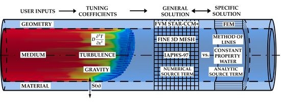
The aim of this paper was to derive and test specialized and fast numerical model of a simple DH pipe that incorporates sharp interface preservation, turbulent diffusion, and detailed radial thermal inertia evaluation caused by the wall.
2. Materials and Methods
This chapter contains a very in-depth description of the mathematics behind the model. In order to ensure that the resultant model is fast, a one-dimensional PDE is used to avoid two spatial derivatives. Here, the incompressibility of the fluid is assumed. Individual variables depend on the position and time as denoted by variables x and t in the following equation:
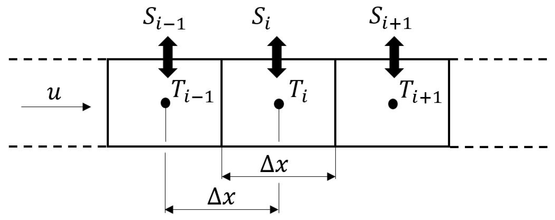
where T is the local cross-sectional temperature of the fluid, u is the axial fluid velocity, D is the axial diffusion coefficient, and S is a source term (dealing with heat flow from inner wall and friction). Because the method of lines is used here, only the spatial derivatives must be discretized. The pipe is divided into na cylindrical volumes, where spatially dependent variables are localized (see Figure 1). Localized temperatures represent the volume-averaged temperature and, localized sources represent the incoming heat from the solid shell divided by the heat capacity of one volume element.
Finite differences are used for discretization. There is a simple relationship between the finite difference schemes for any derivation order (including zero) and given n stencil points [27]:
where c is a vector of the stencil coefficients, m is the derivation order, Z is an n × n matrix such as:
in which xi is the axial position of a stencil point, x0 is the axial position of the point in which the derivative is demanded, and δ represents a vector such as:
The first term on the right-hand side of Equation (1) dealing with advection is discretized in two ways. The first way utilizes Equation (2) directly, which results in the finite difference method (FDM). The second way is based on FVM, where Equation (2) is used for the evaluation of the values at element faces (zero order derivatives). The discretization of the advection part should be good in shock capturing; therefore, 660 tests are conducted to compare this ability among the different schemes. By filling rows with the stencil coefficients, a script written in Julia constructs the matrix A that approximates the derivative operator. Among the input parameters, there is a number of used upwind and downwind stencil points. While filling the first few rows of matrix A, both these parameters are automatically decreased. When filling the last few rows, only the downwind parameter is decreased because of the missing nodes. For example, the maximum number of available upwind nodes at the inlet is one (the boundary temperature). No oscillation is caused by central schemes near the boundaries (unless a central scheme is used explicitly) because the local upwind bias is always preserved (first rows) or increased (last rows). The boundary vector Ain is constructed as well. Both are used to evaluate the pure advection problem in the following form:
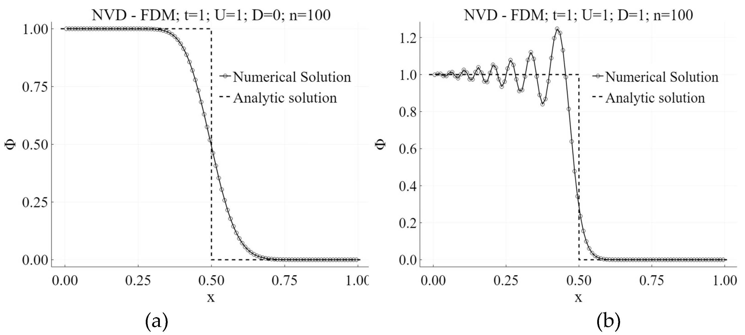
where T is the vector of localized fluid volume temperatures and Tin is the time-dependent scalar representing the inlet (boundary) temperature signal. Problems are solved using normalized variables, and the behavior of the schemes is presented in a normalized variable diagram (NVD). Sundials library is used for solving the problem in time, namely the CVODE algorithm with backward differencing and with relative and absolute tolerances of 10−6. It has an adaptive time step and produces a continuous temperature signal at the outlet by using Hermite interpolation. Examples of NVDs are shown in Figure 2. The diagrams contain hints about the schemes (U and D are the number of upwind and downwind nodes, respectively, and n is a number of volume elements).
It is observed that central schemes have a stronger tendency to oscillate (Figure 2b) and are more computationally expensive than upwind-biased schemes (see Figure 3). Overall, higher order upwind schemes (see Figure 4) seem to show a good compromise between the degree of their oscillation, their ability for shock capturing, and computational expensiveness.
The first order central scheme is used for the construction of B, which is the matrix that approximates the second derivative operator dealing with axial diffusion in Equation (1). Boundary vector Bin allows the calculation of the second derivative at the inlet node as well. Equation (5) is extended and results in Equation (6):
diffusion coefficient D may either be lumped or localized into the form:
The first term in Equation (7) deals with turbulent diffusion. The second term, which is strictly non-negative, corresponds to velocity-independent effects, such as conductive diffusion (which is shown later to be negligible) or spreading due to effects of gravity. If the second term in Equation (7) is neglected, the Equation (6) can be simplified:
where M and Min are the constant matrix operator and boundary vector of the fluid region, respectively. This step should improve the performance of the model. It also makes the Peclét number independent of flow velocity. This means that when proper axial discretization is chosen to ensure non-oscillatory behavior of the method, it is preserved for all velocities of the fluid. Automatic axial discretization, based on values w1,i, is then possible. The weights in Equation (7) allow the tuning of the pipe to mimic a real installation more accurately (similar weighting is possible for the source term as well).
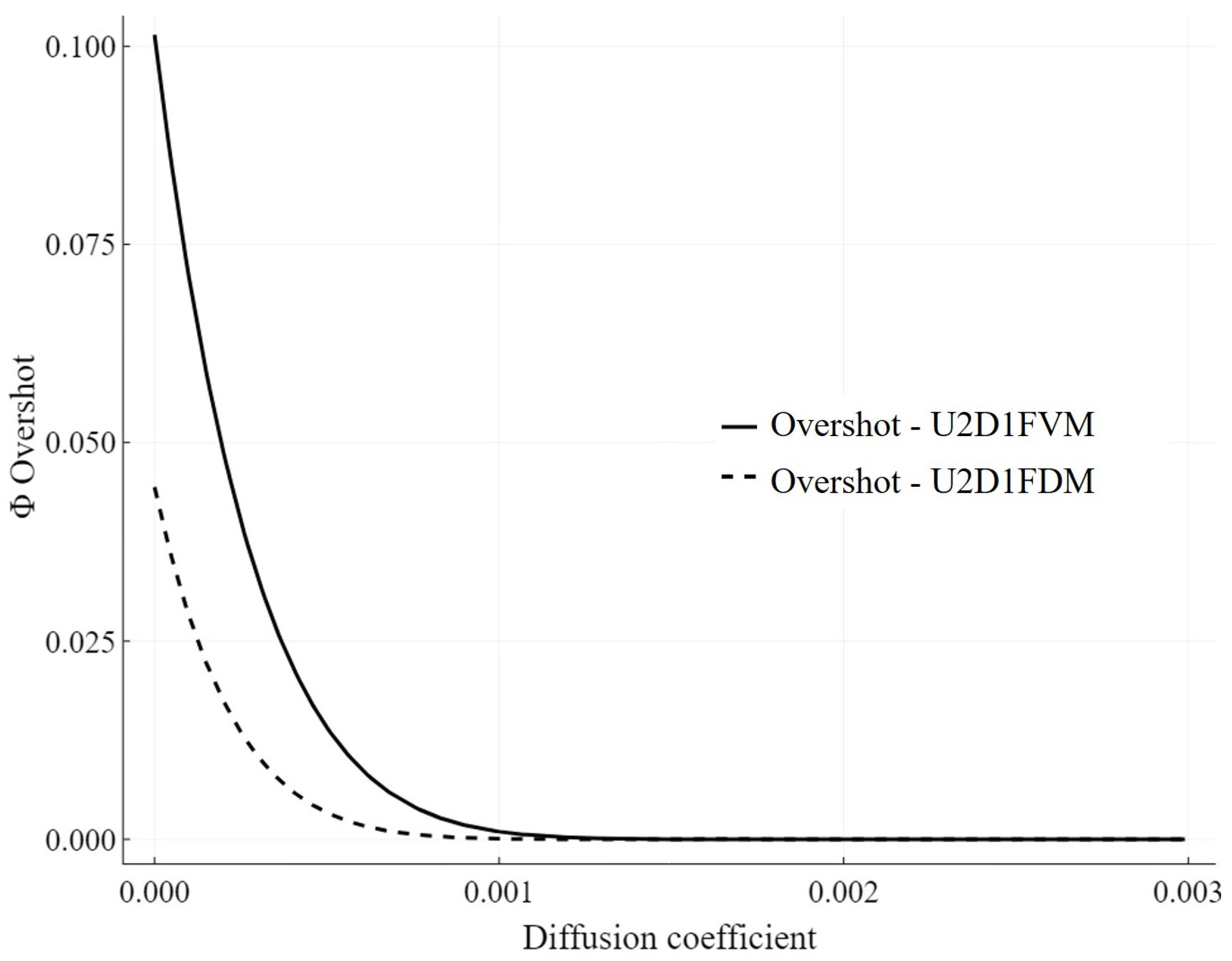
Using the analytic solution to step input in the NVD, the effect of Di on oscillation of Equation (6) is studied. Any value of the numerical solution that is outside of the unit interval is considered to be an overshot caused by oscillation. This is a very simple way to estimate the residual oscillation of Equation (6). FDM is chosen for the model because of its lower oscillations (see Figure 5).
The last term of Equation (1) is more complicated since it must deal with heat dynamics in the solid shells surrounding the pipe. From the fluid viewpoint, the only important value is the inner wall temperature of the first shell. Using publication [6], the Nusselt number for all flow regimes is:
where Re is the Reynolds number, U = Re/1000, fr is the Darcy-Weisbach friction factor, and Pr is the Prandtl Number. The friction factor might be evaluated using the Churchill Equation presented in [7] for all flow regimes:
where
in which ε is the roughness of the inner wall and d1 is the inner diameter. It is a simple step to evaluate the local source term S in the form of a vector:
where Tsn,i,1 represents the inner wall (later first node of the solid region) temperatures of the solid shell, cp is the specific heat capacity of the fluid, ρ is the mass density of the fluid, and λ is the heat conductivity of the fluid.
The time-dependent distribution of temperature in the solid shells affects the axial transients of the heat waves (charging and discharging of the accumulation layers). Tangential and axial heat conductions in the shells are ignored because even when the flow velocity is small, the rate in which the heat is being transported by advection is often much higher than that by conduction. This might be expressed in the form of the Péclet number for conduction in both the fluid:
and the solid (e.g., steel):
As shown, the inner diameters of the pipes or the flow velocities would have to be very small for the conductive axial diffusion to be comparable with advection. This is not common with real applications in the DH systems which also reduces the number of necessary spatial derivatives used in the model. The fluid volumes can be mathematically coupled with one-dimensional models of purely radial heat transfer (later solid segments) described by PDE in the form:
where r is the radial coordinate, Ts,i is the continuous temperature in the solid segment, ρs is the mass density, cps is the specific heat capacity, and λs is the heat conductivity. Equation (15) might be rewritten into the weak form using the shape function V (notice that integrated term in the bracket affects the system only at the boundaries).
The steady state temperature distribution is used as the base for the nodal shape functions:
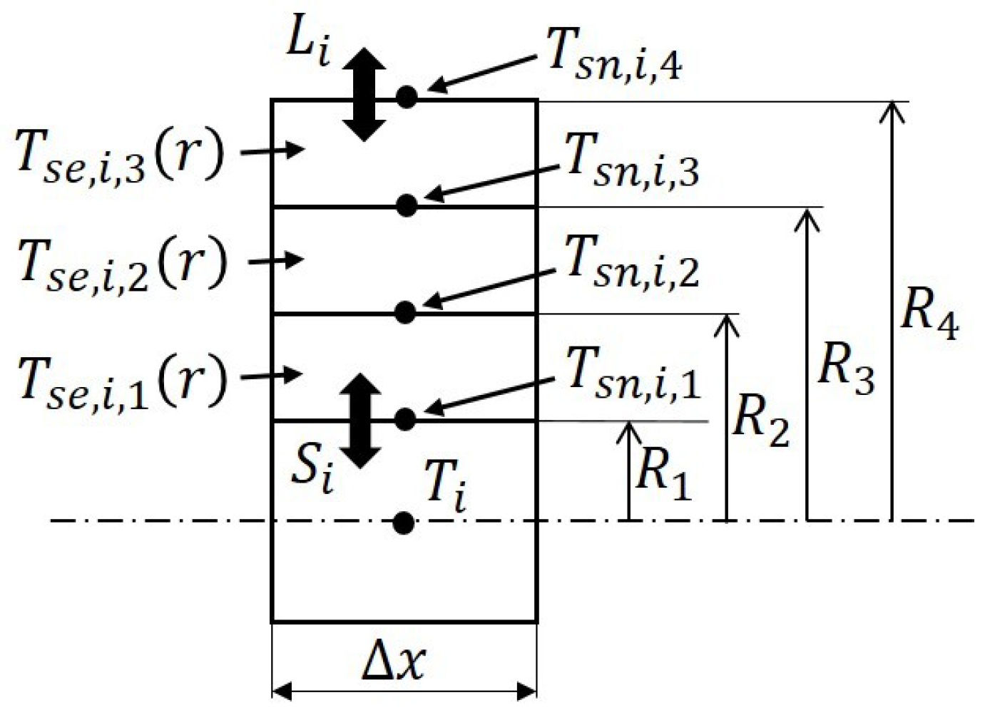
where Tse,i,j are the temperature distributions in the cylindrical elements, Tsn,i,j are nodal temperatures, and Rj are radial coordinates of the nodes. Equation (17) is the solution to the following PDE with given boundary conditions (see also Figure 6):
Nodal shape functions are derived from Equation (17) by considering the effect of one node to the global temperature distribution. Therefore, they take the following piecewise form (notice that boundary nodes are neighboring one element only, so the shape functions have only the appropriate half):
When mass densities and specific heat capacities of the elements are constant, the following integration (according to the left-hand side of Equation (16)) results in discretized heat capacity:
where Csn,j are the nodal heat capacities, ρse,i,j are the mass densities of the elements, and cps,j is the specific heat capacity of the elements. For inside nodes, the integration of (20) results in:
For the boundary near the fluid region, there is only the second term in the bracket (there is no element below), while for the outer boundary node, there is only the first term (there is no element above).
The net heat flow incoming to the nodes in the solid region is (according to the right-hand side of Equation (16)):
where
The nodal net heat flow changes for boundary nodes. For the inner boundary node (here the integrated term in brackets of Equation (16) is replaced by heat flow from fluid to solid), the net heat flow is:
where
and similarly for the outer boundary node:
where the last term represents true heat loss (heat transfer to the environment), αout is the convective heat transfer coefficient at the outer wall, Tair is the ambient temperature and:
Using Equations (16), (21) and (22), the set of ODEs describing heat dynamics in the solid is:
Values in matrix hsn,i,j are nonzero only for values given by Equations (23), (25) and (27). Under such conditions, the following matrices might be constructed:
Using Equations (29) and (30), the relation (28) might be expressed in a form similar to Equation (6):
where Tsn,i are vectors of the nodal temperatures of the solid segments, k is a constant matrix (constructed by Equation (29)) capturing the heat dynamics of the nodes inside segments, and kin,i are the time-dependent vectors containing boundary conditions of the segments. Banded matrices can be used in order to express the dynamics fully in a single equation:
where Tsn is the column vector filled with column vectors Tsn,i, K is the banded square matrix filled with k on its diagonal, and Kin is the time-dependent boundary vector filed with column vectors ksn,i.
This description of the solid region will satisfy the analytic solution completely at steady states but will have a tendency to deviate more with rapid changes of fluid temperature. Individual layers can be further divided into sublayers, which will increase the accuracy during nonstationary events.
3. Results and Discussion
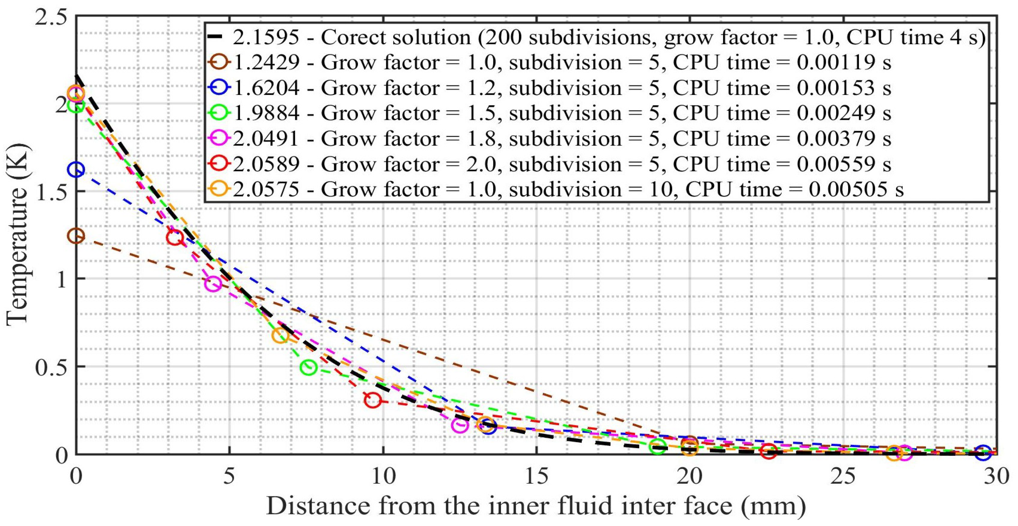
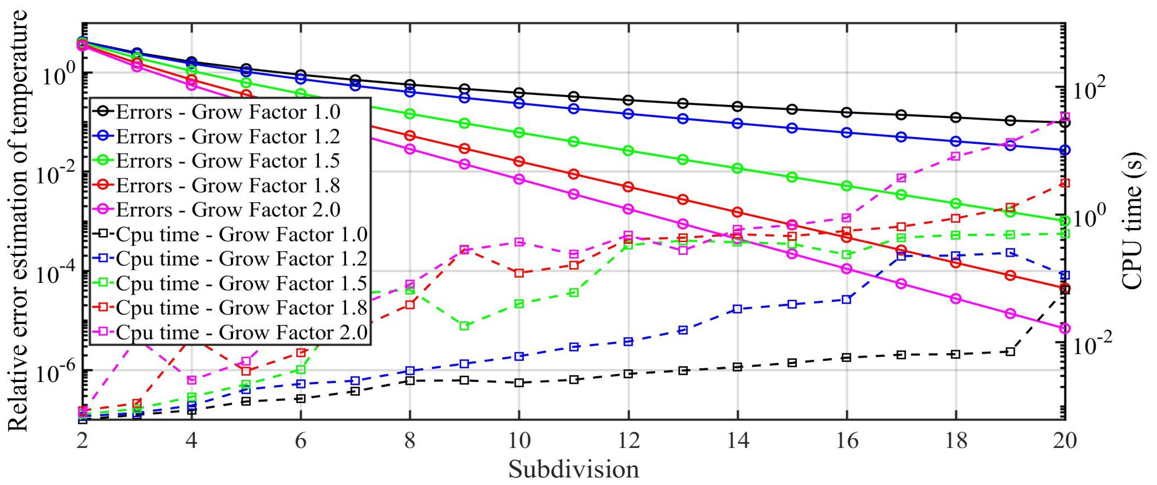
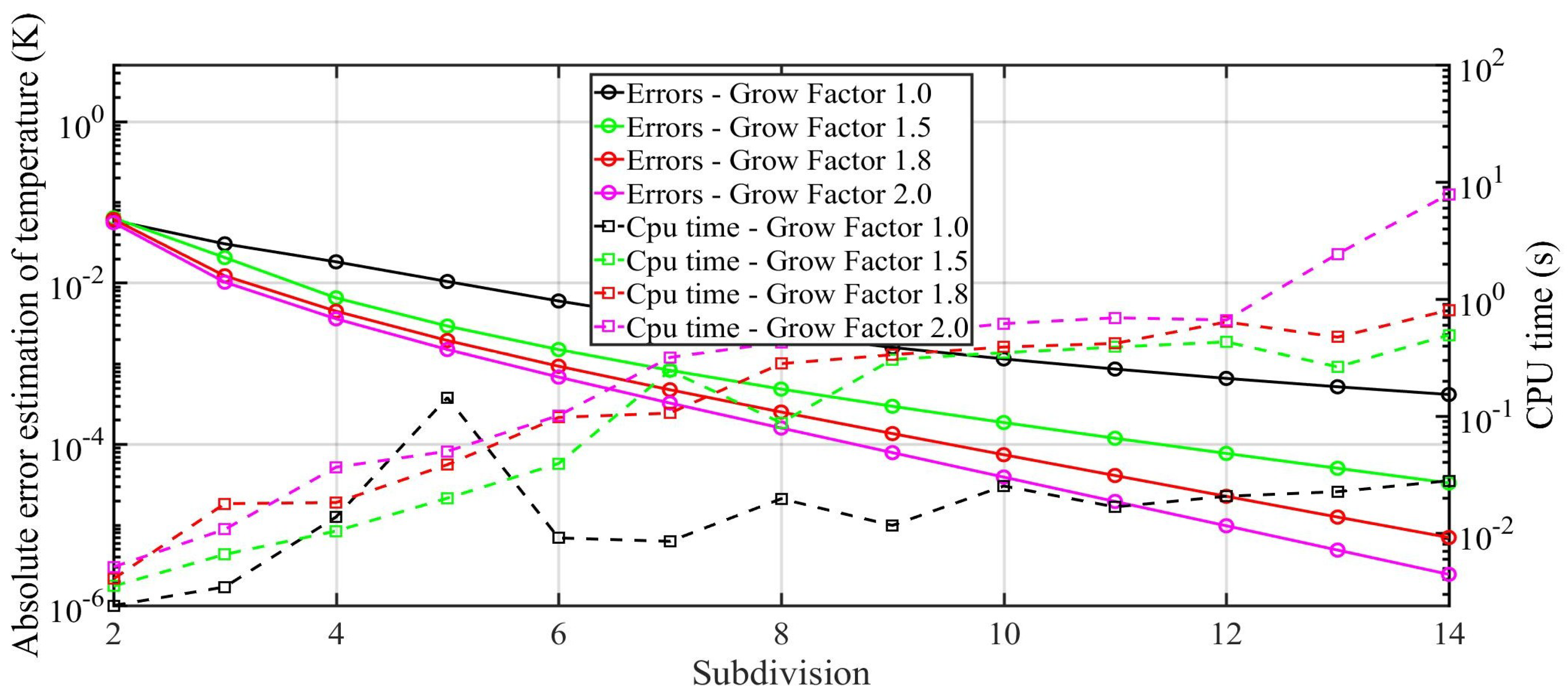
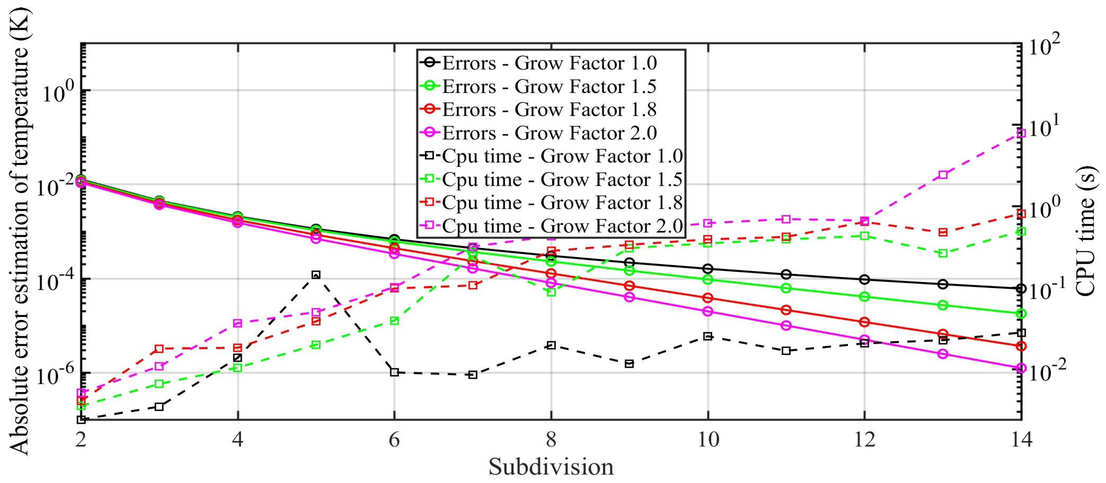
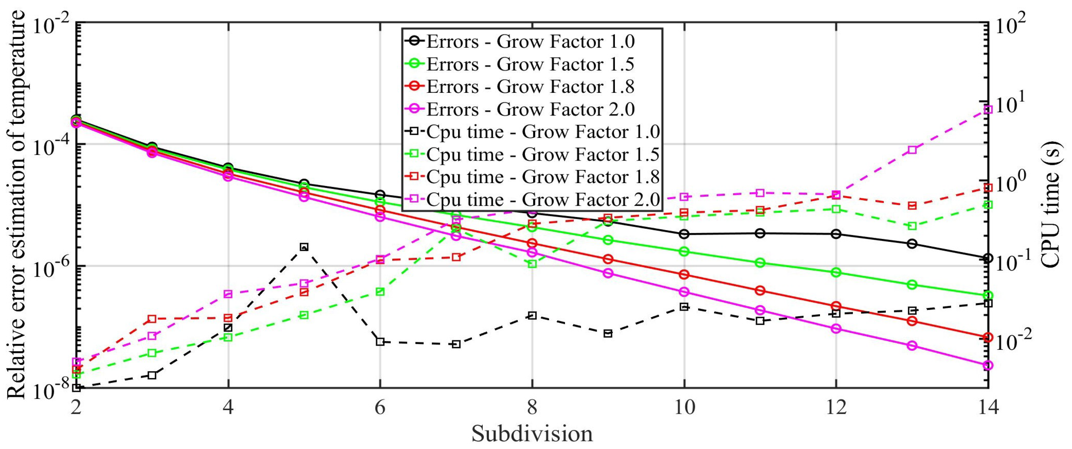
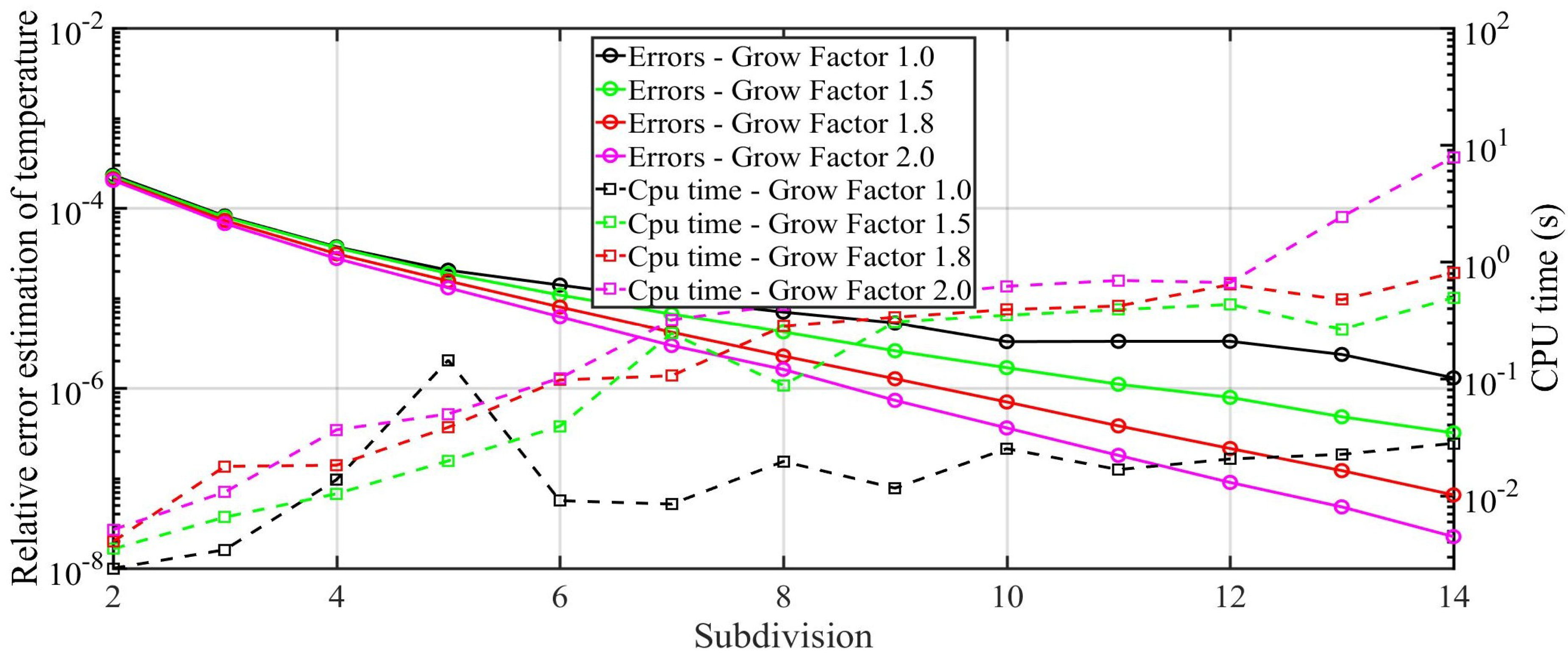
The new model of radial heat transfer is tested for two different cases (see Table 1). The first case is not an actual installation but serves as an example of a case with very strong accumulation. A sudden change in the fluid temperature causes high temporal heat flux between the fluid and the wall. A quick reduction in the heat flux follows due to a rise of the innermost wall surface temperature. The radial elements increasing in size from the inner wall outward should capture this better. Smaller time-steps must be then used to ensure numerical stability. Element sizes are defined by a grow factor. Qualities of the solutions at the innermost piece of the wall are studied using a step change in fluid temperature from 0 to 10 K.
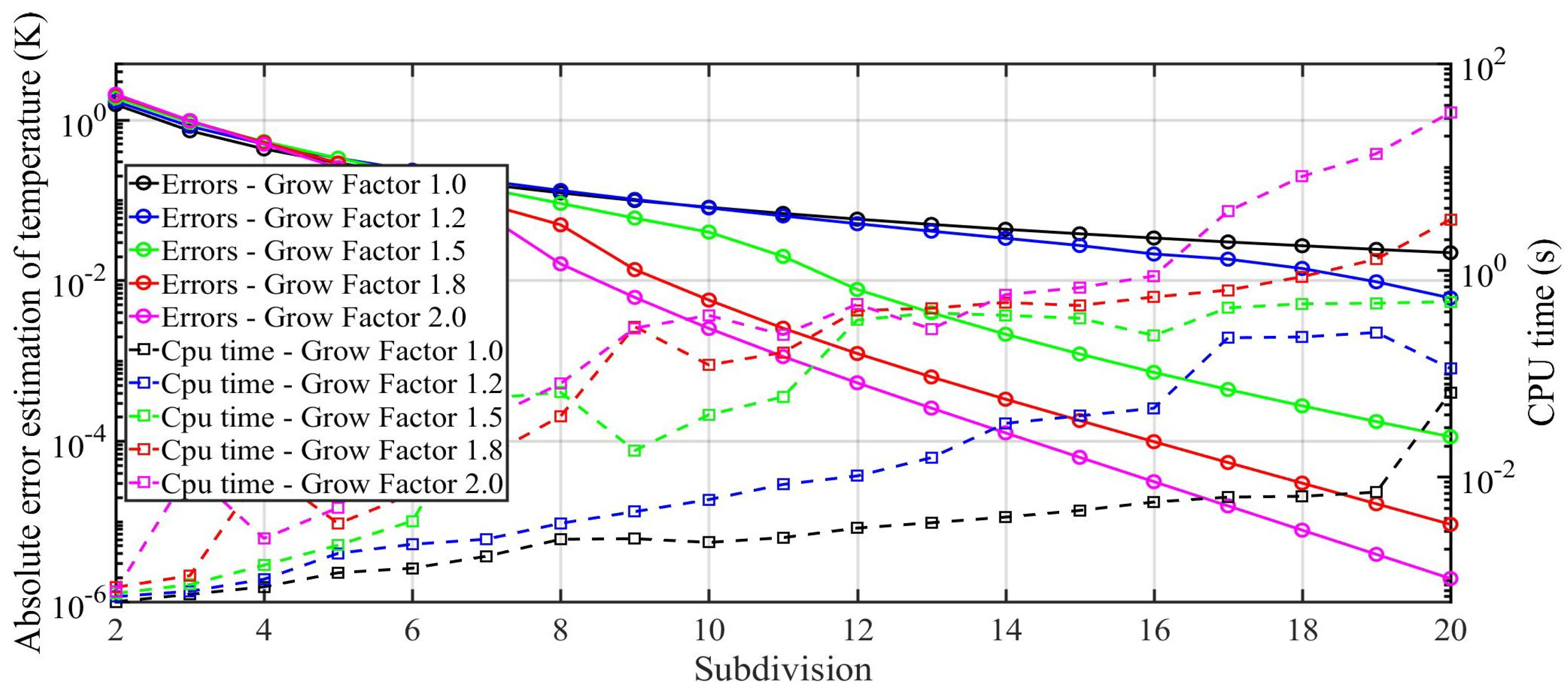
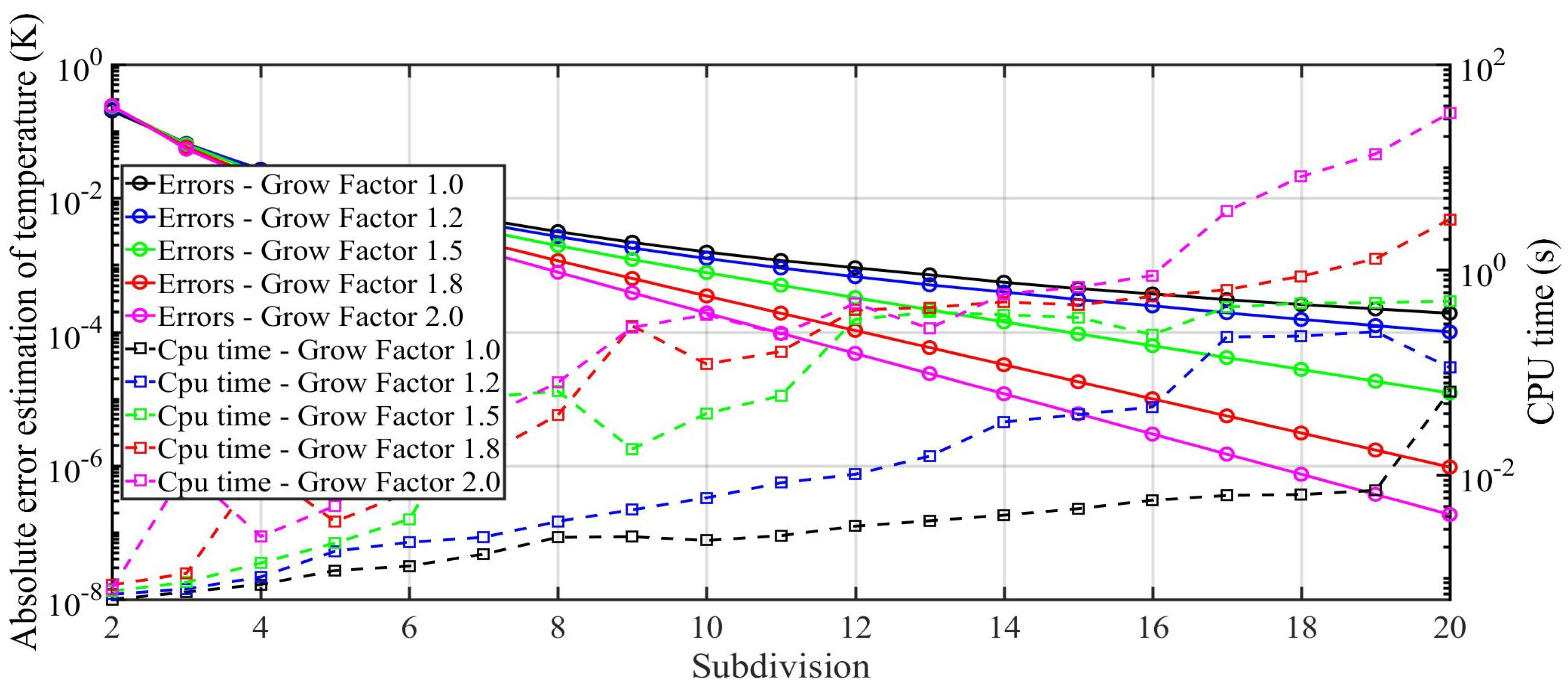
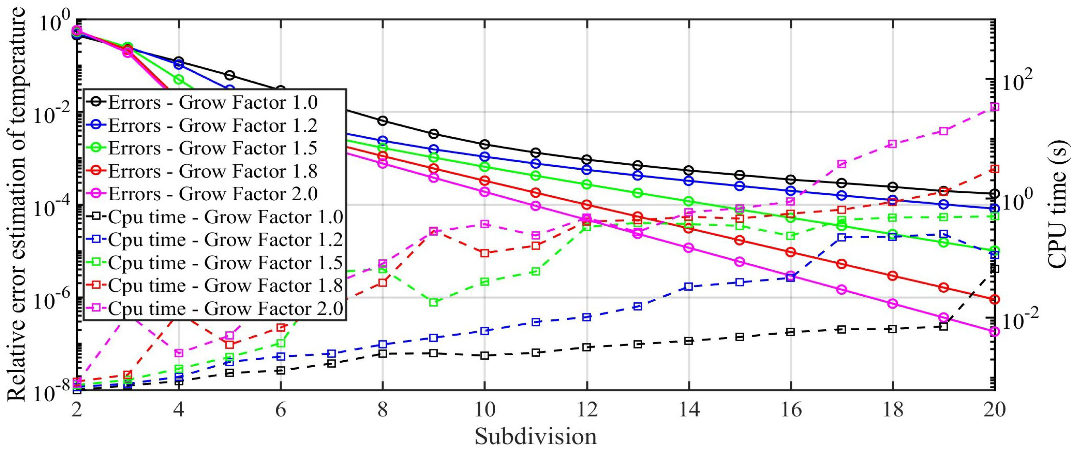
Since the temperature of the fluid steps up to 10 K and the correct inner wall temperature after 10 s is about 2.16 K, the error in heat flux caused by the use of 5 subdivisions (with grow factor 1) would be over 10%. Grow factor 1.0 with 10 subdivisions provides almost equivalent results to an advanced solution that uses grow factor 2.0 with 5 subdivisions, but it is slightly faster (see Figure 7). The thin wall in the second case behaves much better. It produces solutions accurate enough even with lower subdivisions (compare Figure 8, Figure 9, Figure 10 and Figure 11 with Figure 12, Figure 13, Figure 14 and Figure 15). This ensures good computational speed for such arrangements. To further estimate the accuracy of the new radial model for the case with strong accumulation, the maximal errors are estimated using temperature refinements between two consecutive levels of subdivision (see Figure 8, Figure 9, Figure 10 and Figure 11). The whole event of heat recharging is used (7200 s). A tolerance of 10−12 is chosen to ensure that the time stepping method can always take advantage of a superior spatial discretization.
The errors in the second case for lower subdivisions are equivalent to errors in the first case for high subdivisions. This is because the inertia of the thin wall is not significant. The relative errors of the inner and outer walls are almost the same (Figure 13 and Figure 14).
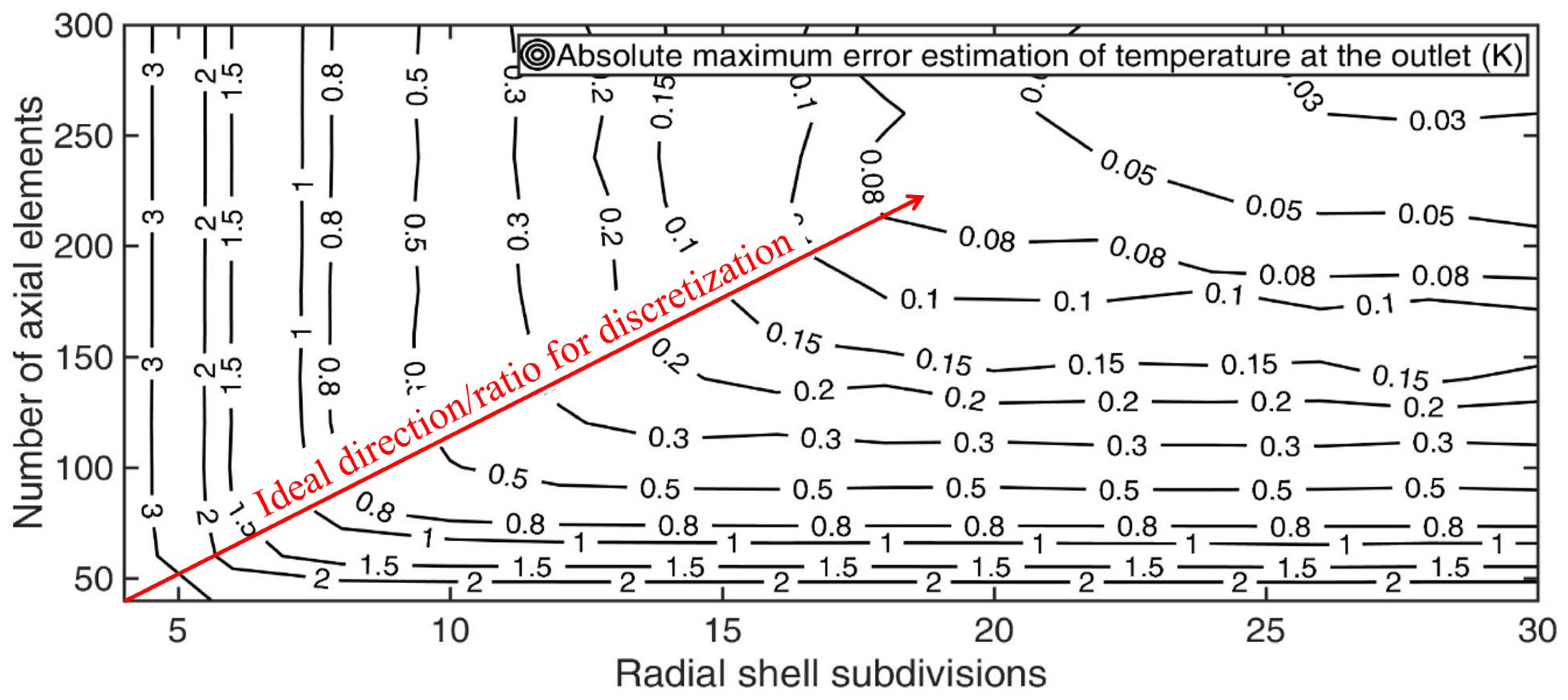
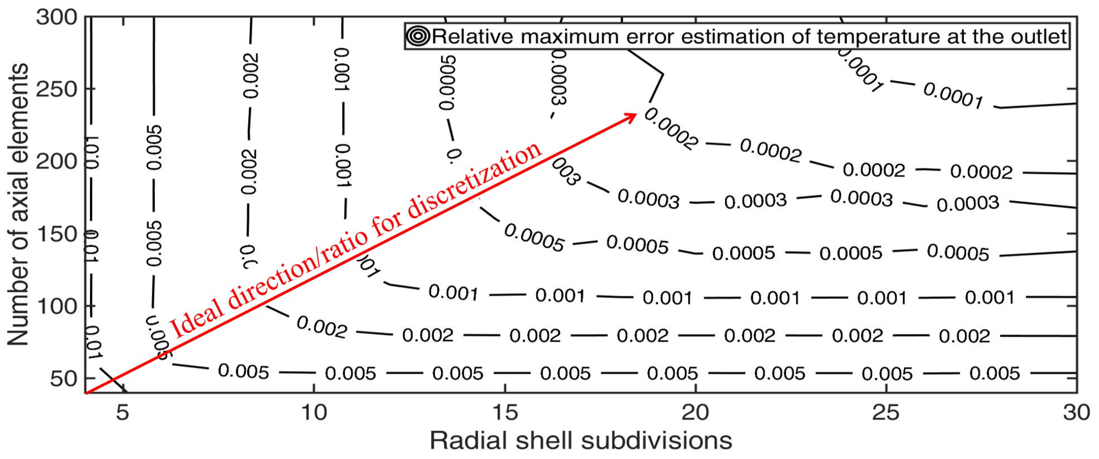
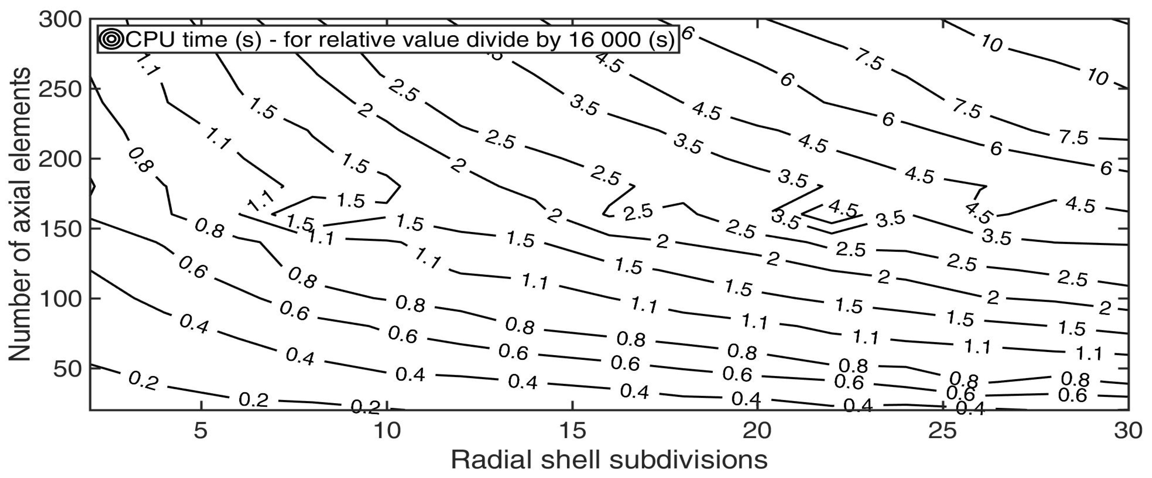
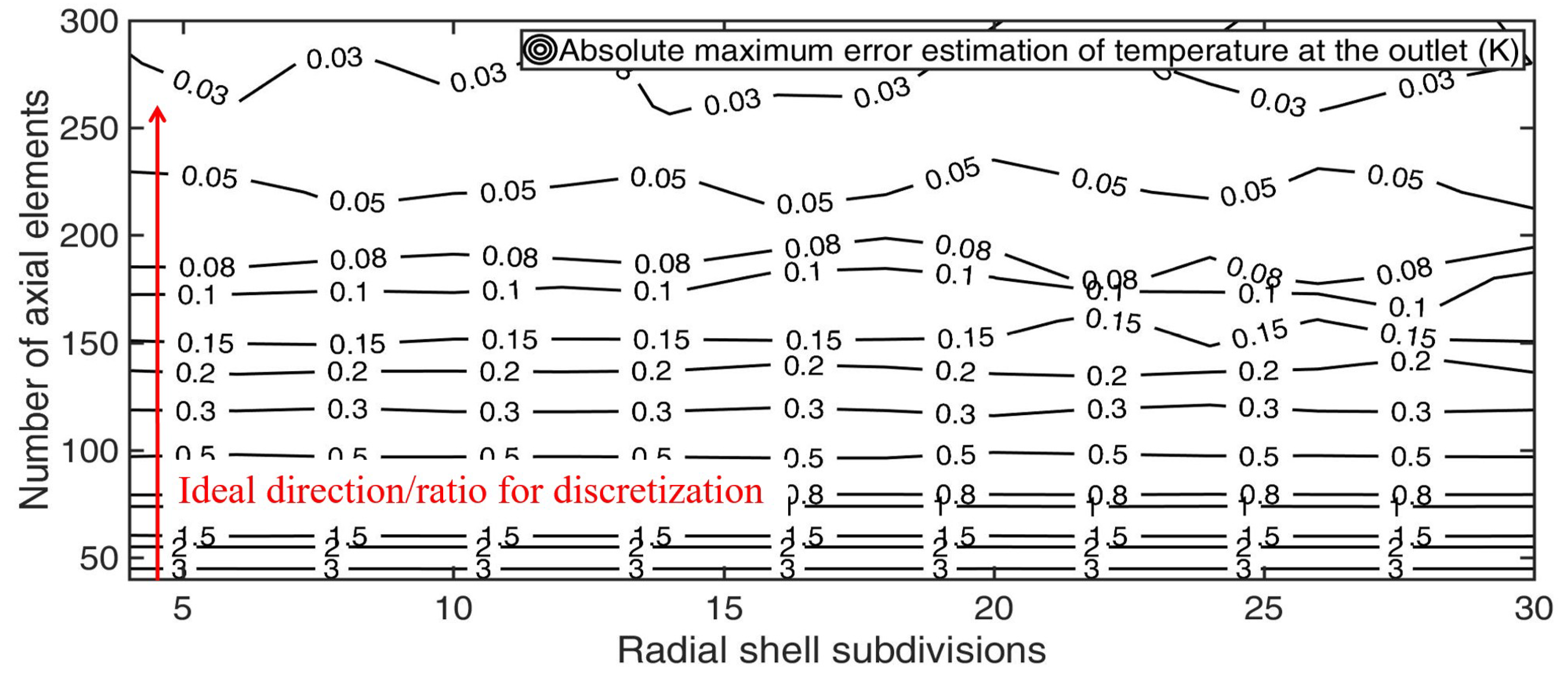
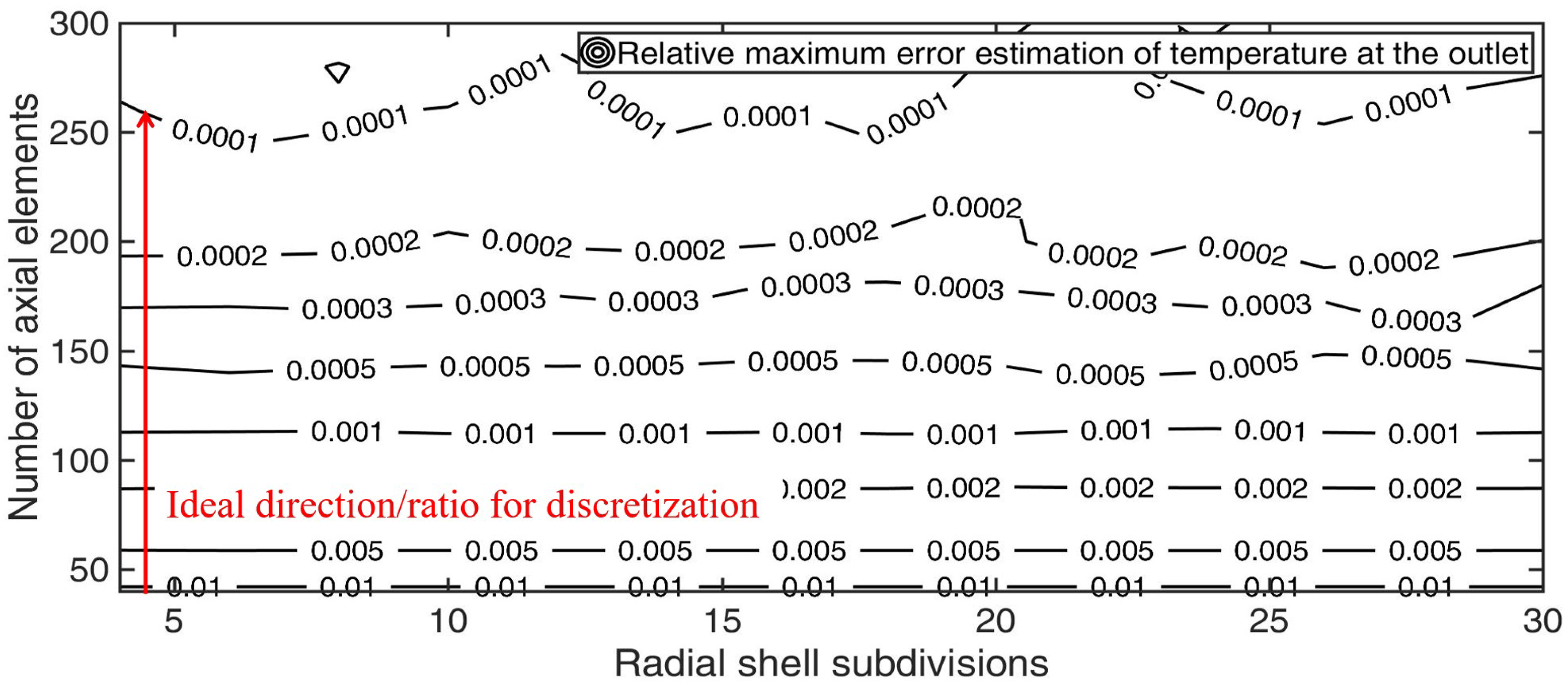
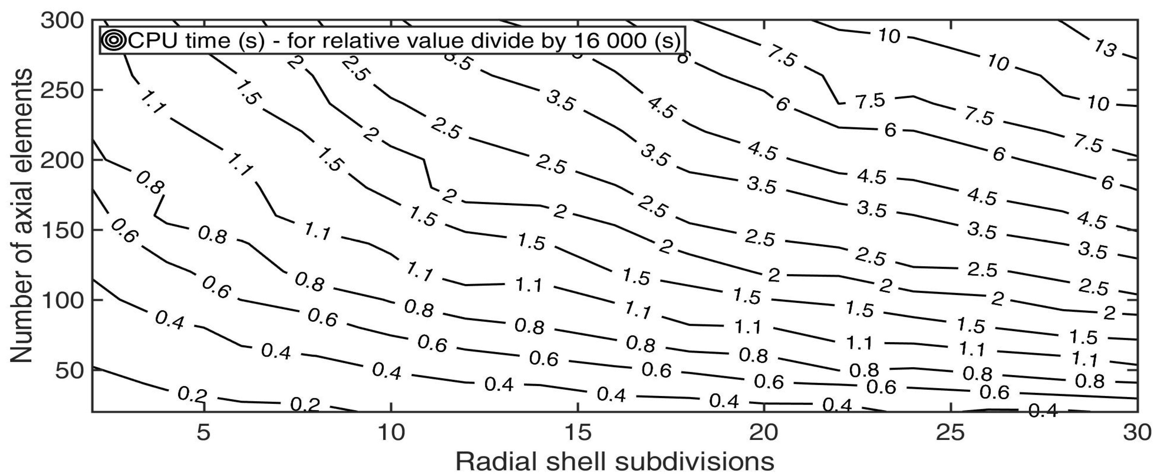
The composite model of the pipe written in OpenModelica is tested in a similar way (Julia was significantly slower here, possibly due to the use of numerical jacobians instead of symbolic ones). The 100 m long pipe with a cross-section corresponding to the first case of the previous test set is initialized with a temperature of 323.15 K. After steady-state is reached, a 30 K rise and drop in the inlet temperature generate the transient process. The duration of the tests was 16,000 s. The tolerance is set to 10−6, and the values are saved every 3 s. Error estimations are evaluated using a discrete gradient (backward differencing) between the set of discretization. Using contours, the “willingness to refine maximal errors” of the model can be mapped (see Figure 16 and Figure 17). The computational time can be mapped directly (see Figure 18).
Similar tests for the second case clearly demonstrate the independence on the radial number of subdivisions (see Figure 19 and Figure 20). There is nothing to be refined in the radial direction. Further subdivisions only take more computational time (see Figure 21). The higher computational time in the right top corner of Figure 21 is caused by smaller time steps to ensure numerical stability.
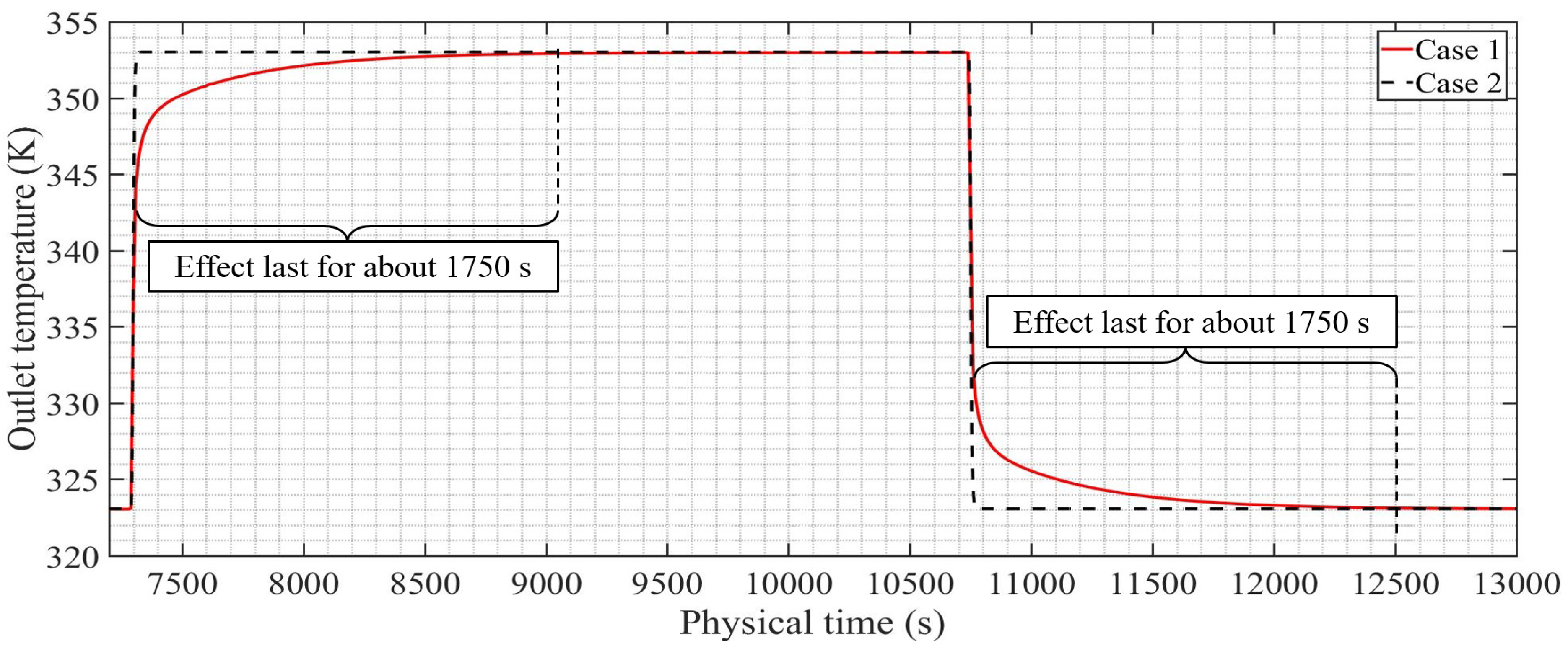
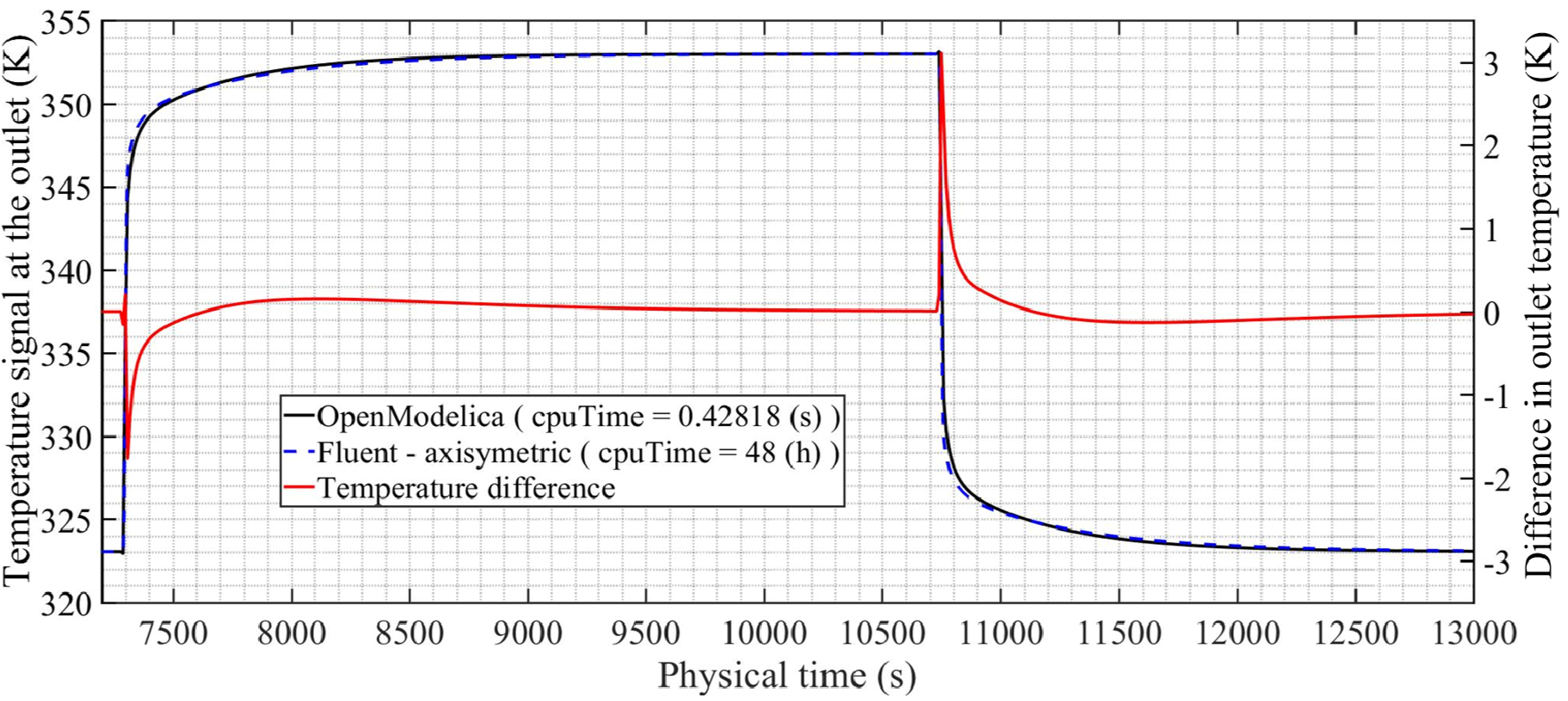
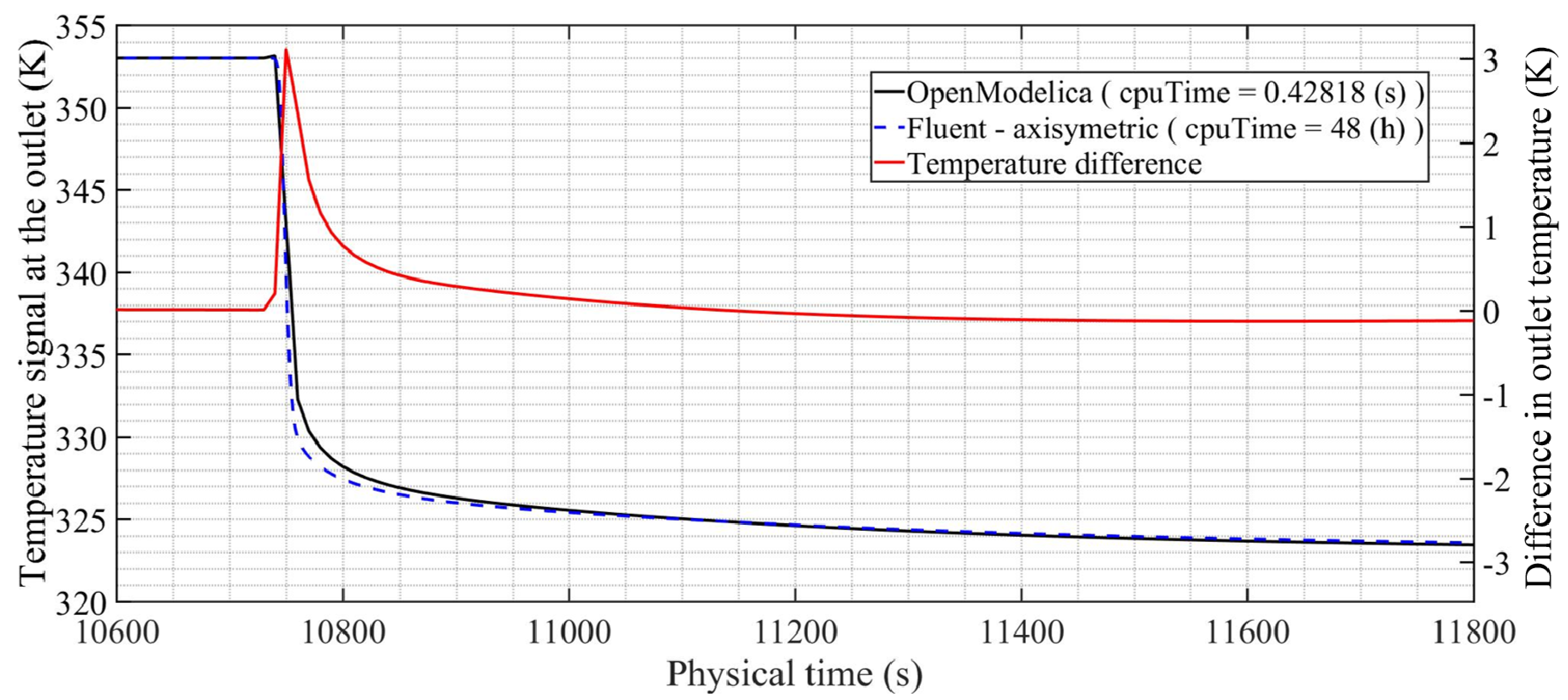
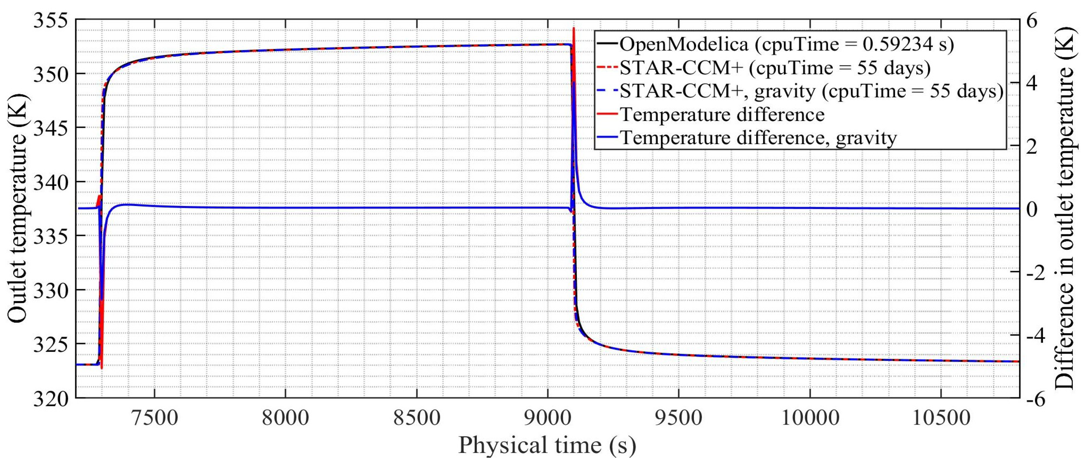
The Figure 22 demonstrates the effect of the strong accumulation using the outlet temperature perspective. The above results deal with the model alone. Unfortunately, real data were not available to the authors to validate the model properly. The model is at least compared (partially validated) to a very fine model developed in Fluent (axisymmetric 2D in Figure 23 and Figure 24) and STAR-CCM+ (fully 3D in Figure 25 and Figure 26). The tolerance of the new model was lowered to 10−5 and samples were saved every 10 s to demonstrate the effectiveness of the new model. The time span of the simulation was 16,000 s.
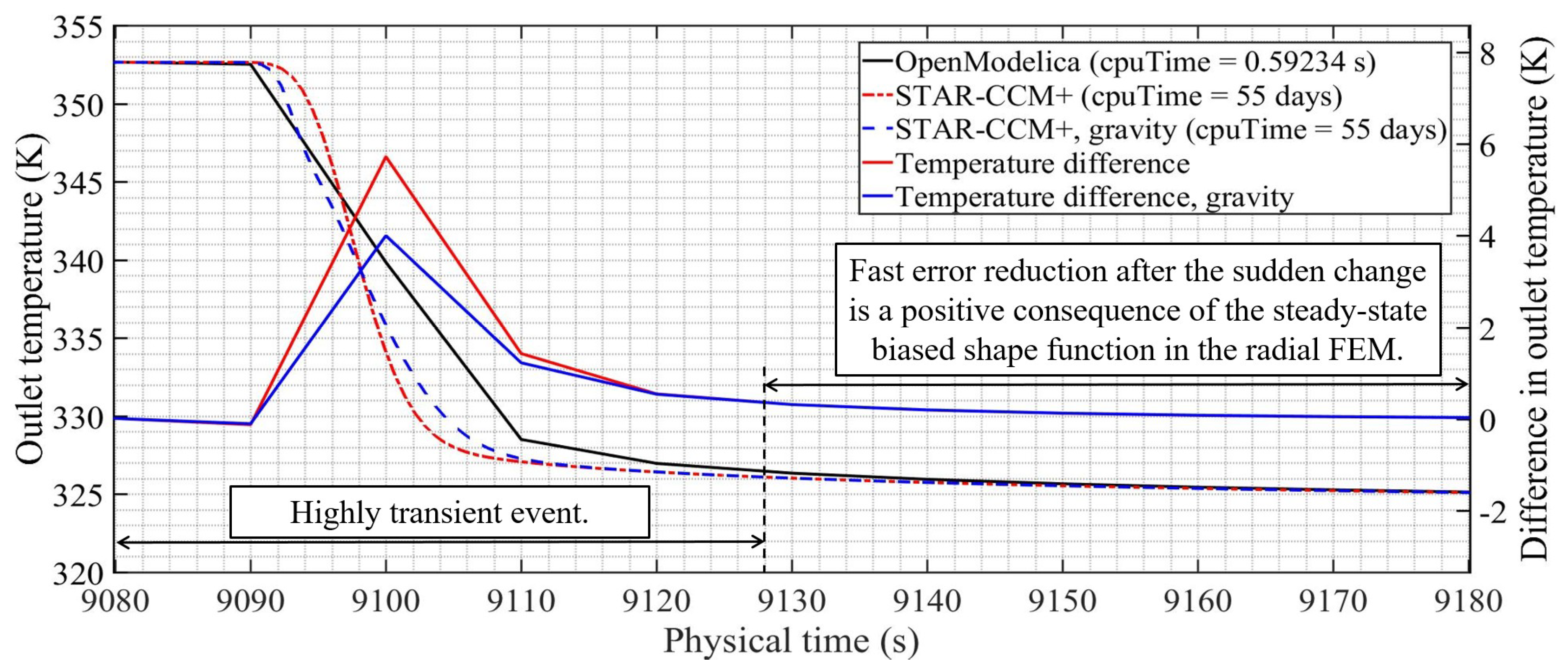
Although the maximal temperature difference is higher than the model from STAR-CCM+, the temperature difference falls close to zero quicker than the model from Fluent. The effect of gravity on wave propagation is such that it behaves as additional axial diffusion, which can be tuned up by adjusting weights in Equation (7). Figure 26 shows this fact by the more time-spread rise in temperature at the outlet. Figure 27 and Figure 28 show how the gravity spreads the temperature front in the STAR-CCM+ model 7 s after both hot and cold waves entered the pipe.
The comparison of the new model with the very fine numerical counterparts shows that the new model overestimates the wave to reach the outlet slightly later (asymmetric peaks in temperature difference in the Figure 23, Figure 24, Figure 25 and Figure 26). This might be caused by the fact that the temperature and velocity profiles in the new model are considered to be fully developed right from the beginning, while with the very fine counterparts they are not.
4. Summary of the Results
- The shape function used in the radial model as well as the use of analytic description of heat exchange between the fluid and the inner wall surface ensures that the solution of the new model agree with the analytic solution completely even for the roughest radial discretization (also visible through fast stabilization in Figure 22 after the sudden temperature change).
- The new model allows simple modeling of circular pipes with an arbitrary number of shells and their material properties (e.g., a steel wall followed by insulation and a plastic shell). All shells then consider radial dynamic effects based on the newly derived radial model, and OpenModelica’s marching algorithm automatically adapts the time step to ensure its numerical stability.
- Although elements growing in size in the radial direction better capture the sudden changes of temperature, the necessity of smaller time steps to ensure the stability of the marching algorithm completely negates this advantage (compare the CPU time in Figure 7) and makes the uniform mesh more preferable.
- With the preferred use of the uniform mesh in the radial model, the thick wall has to be modeled with higher number of elements, while the thin wall is captured well with very few or even single element (compare error estimations for grow factor 1 in Figure 8, Figure 9, Figure 10, Figure 11, Figure 12, Figure 13, Figure 14 and Figure 15 or the error maps in Figure 16 and Figure 19).
- The use of the method of lines and appropriate algorithm with adaptable time step makes the precision easily tradable for computation time, without the necessity to focus on the numerical stability conditions of the composite model (trading the capturing of the transients for CPU time, the steady-states will be captured accurately even with rough radial meshes).
- There are regions in which a sole improvement of the mesh in one direction will not result in superior solution (e.g., see the region of 100 axial and 20 radial elements in Figure 16, where sole improvement of radial discretization does not lower errors). There is, however, an ideal direction for the discretization in each case.
- Figure 22 shows how does strong thermal inertia of the wall affect the outlet temperature in idealized case (the effect lasts approximately for half an hour for the thick steel wall).
- Maximal deviation in outlet temperature in comparison with Fluent (2D) is about 3 K.
- Maximal deviation in outlet temperature in comparison with STAR-CCM+ (3D) is about 6 K for the case without gravity and 4 K for the case that includes gravity.
- During all simulations, positive weights in the definition of axial diffusion are deployed, which shows that turbulent axial mixing plays a role in thermal wave propagation.
- Presence of gravity in fully horizontal pipes acts as additional axial diffusion from the viewpoint of cross-sectional temperature average (comparison of the two curves from STAR-CCM+ in Figure 26).
- Relative simulation time of the new model for a single 100 m long pipe with strong accumulation is approximately in order of 3.75 × 10⁻⁵.
- A simple quasi-static evaluation of the pressure losses (the friction coefficient is already being evaluated during thermal simulation) would allow the use of the new model for simulation of whole grids with automatic mass flows evaluation in each branch (e.g., OpenModelica connector definition includes Kirchhoff laws by default).
5. Conclusions
This paper deals with transients in circular pipes, where the accumulation of heat into surrounding material has been considered in detail. Model is a combination of the analytic description of a heat transfer between the fluid and the solid wall, simple advection scheme, turbulent diffusion, and a finite element scheme dealing with the circular wall in which the shape functions are based on the steady-state solution. Method of lines is used for time integration. The new model represents an effective numerical solution to the thermal wave propagation problem, which includes advanced evaluation of thermal inertia of the pipe’s wall and the axial diffusion that is caused by turbulence. The diffusion coefficient evaluation is mainly proportional to flow velocity.
Overall, it can be said that strong accumulation affects the thermal wave propagation for a stretched period of time in comparison with the non-accumulation case. The effect of the re-accumulation is not only dependent on the pure amount of re-accumulated heat, but also on the particular way this event happens. In other words, to capture the event accurately is to focus on the proper evaluation of the innermost surface temperature of the pipe’s wall because it directly affects the rate in which the temperature of the fluid changes. The discretization of both axial and radial direction must go hand in hand to improve the solution. During comparison with the fine models from Fluent and STAR-CCM+, deployment of positive weights in the diffusion coefficient evaluation are always necessary to match the simulated data. This means that turbulent diffusion plays a role in temperature wave propagation. Presence of physical diffusion also reduces unphysical oscillation on sharp interfaces. Gravity is shown to resemble the behavior of an additional axial diffusion as well. The new model resembles the transient behavior of the accumulating pipe wall with highly comparable results to the equivalent, very fine models from Fluent and STAR-CCM+, which should represent the ideal physics-based modeling. The validation with a branched real system needs to be done in the future.
The composite model had run faster in OpenModelica than in Julia possibly because of a non-optimized jacobian evaluation. It might be possible to speed up the Julia execution using function definition macros from Differential Equations package, which could be able to derive symbolic jacobian automatically. The model can be extended by pressure loss evaluation, which would allow simulation of whole DH grids based on Kirchhoff laws. Regularization of mass flows would be necessary here to avoid singularities (division by zero) in the nodes.
The future work should aim at a self-identification algorithm using inlet/outlet temperature signals from real installations to calibrate the appropriate weights in the model. It may be possible to generalize the approach for more complex configurations, such as twin-pipes, buried pipes, and so on. An optimization algorithm can be used to find the matrix coefficient describing the radial heat dynamics. A background from machine learning may be utilized for such an endeavor. The scaling of the new model, when used for simulation of whole grids with automatic mass flow evaluation in each branch based on the pressure drops between individual nodes, is also part of the future work.
Author Contributions
Conceptualization, L.K.; Data curation, L.K. and R.C.; Formal analysis, L.K.; Funding acquisition, J.P.; Investigation, L.K.; Methodology, L.K. and R.C.; Project administration, J.P.; Software, L.K. and R.C.; Supervision, J.P.; Validation, L.K. and R.C.; Visualization, L.K., R.C., and J.P.; Writing-original draft, L.K. and J.P.; Writing-review & editing, L.K.
Funding
This paper has been supported by the project “Computer Simulations for Effective Low-Emission Energy” funded as project No. CZ.02.1.01/0.0/0.0/16_026/0008392 by Operational Programme Research, Development and Education, Priority axis 1: Strengthening capacity for high-quality research.
Conflicts of Interest
The authors declare no conflict of interest.
References
- Lund, H.; Werner, S.; Wiltshire, R.; Svendsen, S.; Thorsen, J.E.; Hvelplund, F.; Mathiesen, B.V. 4th Generation District Heating (4GDH). Integrating smart thermal grids into future sustainable energy systems. Energy 2014, 68, 1–11. [Google Scholar] [CrossRef]
- Lund, R.; Østergaard, D.S.; Yang, X.; Mathiesen, B.V. Comparison of Low-temperature District Heating Concepts in a Long-Term Energy System Perspective. Int. J. Sustain. Energy Plan. Manag. 2017, 12, 5–18. [Google Scholar] [CrossRef]
- Connolly, D.; Lund, H.; Mathiesen, B.V.; Werner, S.; Möller, B.; Persson, U.; Boermans, T.; Trier, D.; Østergaard, P.A.; Nielsen, S. Heat Roadmap Europe: Combining district heating with heat savings to decarbonise the EU energy system. Energy Policy 2014, 65, 475–489. [Google Scholar] [CrossRef]
- Lund, H.; Østergaard, P.A.; Connolly, D.; Ridjan, I.; Mathiesen, B.V.; Hvelplund, F.; Thellufsen, J.Z.; Sorknæs, P. Energy Storage and Smart Energy Systems. Int. J. Sustain. Energy Plan. Manag. 2016, 11, 3–14. [Google Scholar] [CrossRef]
- Vandermeulen, A.; van der Heijde, B.; Helsen, L. Controlling district heating and cooling networks to unlock flexibility: A review. Energy 2018, 151, 103–115. [Google Scholar] [CrossRef]
- Abraham, J.P.; Sparrow, E.M.; Tong, J.C.K. Heat transfer in all pipe flow regimes: Laminar, transitional/intermittent, and turbulent. Int. J. Heat Mass Transf. 2009, 52, 557–563. [Google Scholar] [CrossRef]
- Churchill, S.W. Friction factor Equations spans all fluid-flow regimes. Chem. Eng. 1977, 84, 91–92. [Google Scholar]
- Wang, J.; Zhou, Z.; Zhao, J. A method for the steady-state thermal simulation of district heating systems and model parameters calibration. Energy Convers. Manag. 2016, 120, 294–305. [Google Scholar] [CrossRef]
- Fang, T.; Lahdelma, R. State estimation of district heating network based on customer measurements. Appl. Therm. Eng. 2014, 73, 1211–1221. [Google Scholar] [CrossRef]
- Benonysson, A. Dynamic Modelling and Operational Optimization of District Heating Systems; Lab. of Heating and Air Conditioning, Technical University of Denmark: Lyngby, Denmark, 1991. [Google Scholar]
- Zheng, J.; Zhou, Z.; Zhao, J.; Wang, J. Function method for dynamic temperature simulation of district heating network. Appl. Therm. Eng. 2017, 123, 682–688. [Google Scholar] [CrossRef]
- van der Heijde, B.; Fuchs, M.; Ribas Tugores, C.; Schweiger, G.; Sartor, K.; Basciotti, D.; Müller, D.; Nytsch-Geusen, C.; Wetter, M.; Helsen, L. Dynamic Equation-based thermo-hydraulic pipe model for district heating and cooling systems. Energy Convers. Manag. 2017, 151, 158–169. [Google Scholar] [CrossRef]
- Chertkov, M.; Novitsky, N.N. Thermal Transients in District Heating Systems. Energy 2018. [Google Scholar] [CrossRef] [Green Version]
- Duquette, J.; Rowe, A.; Wild, P. Thermal performance of a steady state physical pipe model for simulating district heating grids with variable flow. Appl. Energy 2016, 178, 383–393. [Google Scholar] [CrossRef]
- Benonysson, A.; Bohm, B.; Ravn3t, H.F. Operational optimization in a district heating system. Energy Convers. Manag. 1995, 36, 297–314. [Google Scholar] [CrossRef]
- Stevanovic, V.D.; Zivkovic, B.; Prica, S.; Maslovaric, B.; Karamarkovic, V.; Trkulja, V. Prediction of thermal transients in district heating systems. Energy Convers. Manag. 2009, 50, 2167–2173. [Google Scholar] [CrossRef]
- Wang, H.; Meng, H. Improved thermal transient modeling with new 3-order numerical solution for a district heating network with consideration of the pipe wall’s thermal inertia. Energy 2018, 160, 171–183. [Google Scholar] [CrossRef]
- Leonard, B.P. Universal Limiter for Transient Interpolation Modeling of the Advective Transport Equations: The ULTIMATE Conservative Difference Scheme; NASA Lewis Research Center: Cleveland, OH, USA, 1988.
- Leonard, B.P. A stable and accurate convective modelling procedure based on quadratic upstream interpolation. Comput. Methods Appl. Mech. Eng. 1979, 19, 59–98. [Google Scholar] [CrossRef]
- Grosswindhager, S.; Voigt, A.; Kozek, M. Linear Finite-Difference Schemes for Energy Transport in District Heating Networks. In Proceedings of the 2nd International Conference on Computer Modelling and Simulation, Mumbai, India, 7–9 January 2011; pp. 5–7. [Google Scholar]
- Neumann, L.E.; Šimůnek, J.; Cook, F.J. Implementation of quadratic upstream interpolation schemes for solute transport into HYDRUS-1D. Environ. Model. Softw. 2011, 26, 1298–1308. [Google Scholar] [CrossRef]
- Modelica Association Modelica Language Specification Documentation Release 3.3 Revision 1 (+ Sphinx conversion). Available online: https://media.readthedocs.org/pdf/modelica/numbered/modelica.pdf (accessed on 9 November 2018).
- Kudela, L. OpenModelicaFromMatlab. Available online: https://github.com/LiborKudela/OpenModelicaFromMatlab (accessed on 9 November 2018).
- Bezanson, J.; Edelman, A.; Karpinski, S.; Shah, V.B. Julia: A Fresh Approach to Numerical Computing. SIAM Rev. 2017, 59, 65–98. [Google Scholar] [CrossRef] [Green Version]
- Rackauckas, C.; Nie, Q. DifferentialEquations.jl—A Performant and Feature-Rich Ecosystem for Solving Differential Equations in Julia. J. Open Res. Softw. 2017, 5. [Google Scholar] [CrossRef]
- Hindmarsh, A.C.; Brown, P.N.; Grant, K.E.; Lee, S.L.; Serban, R.; Shumaker, D.E.; Woodward, C.S. SUNDIALS: Suite of Nonlinear and Differential/Algebraic Equation Solvers. ACM Trans. Math. Softw. 2005, 31, 363–396. [Google Scholar] [CrossRef]
- Taylor, C. Finite Difference Coefficients Calculator. Available online: http://web.media.mit.edu/~crtaylor/calculator.html (accessed on 10 November 2018).
Figure 1.
Division of pipe’s fluid region into volumes, with localized spatial dependent variables.

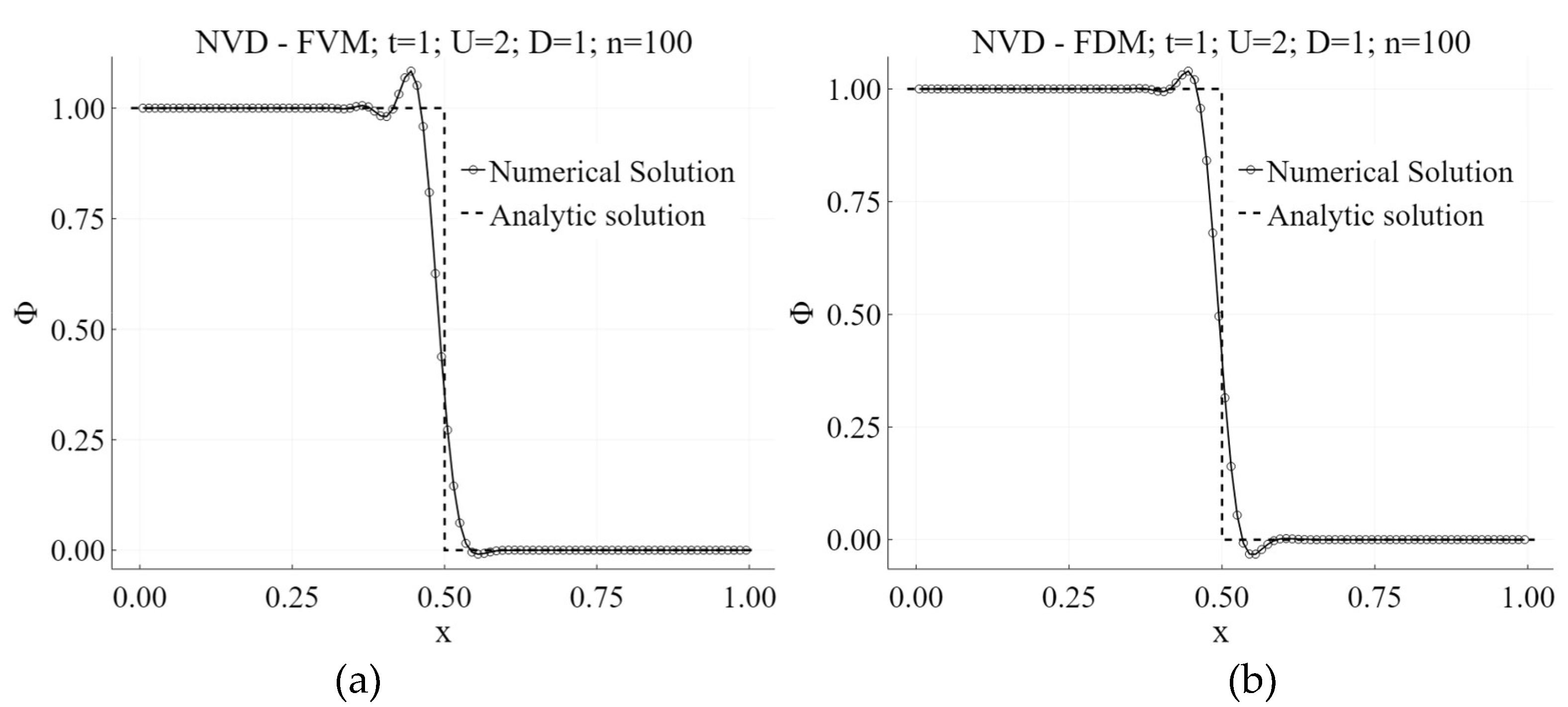
Figure 2.
Examples of bad-behaving advection schemes. (a): Low order upwind biased scheme causes a lot of numerical diffusion; (b): Low order central scheme is being too oscillatory.
Figure 2.
Examples of bad-behaving advection schemes. (a): Low order upwind biased scheme causes a lot of numerical diffusion; (b): Low order central scheme is being too oscillatory.

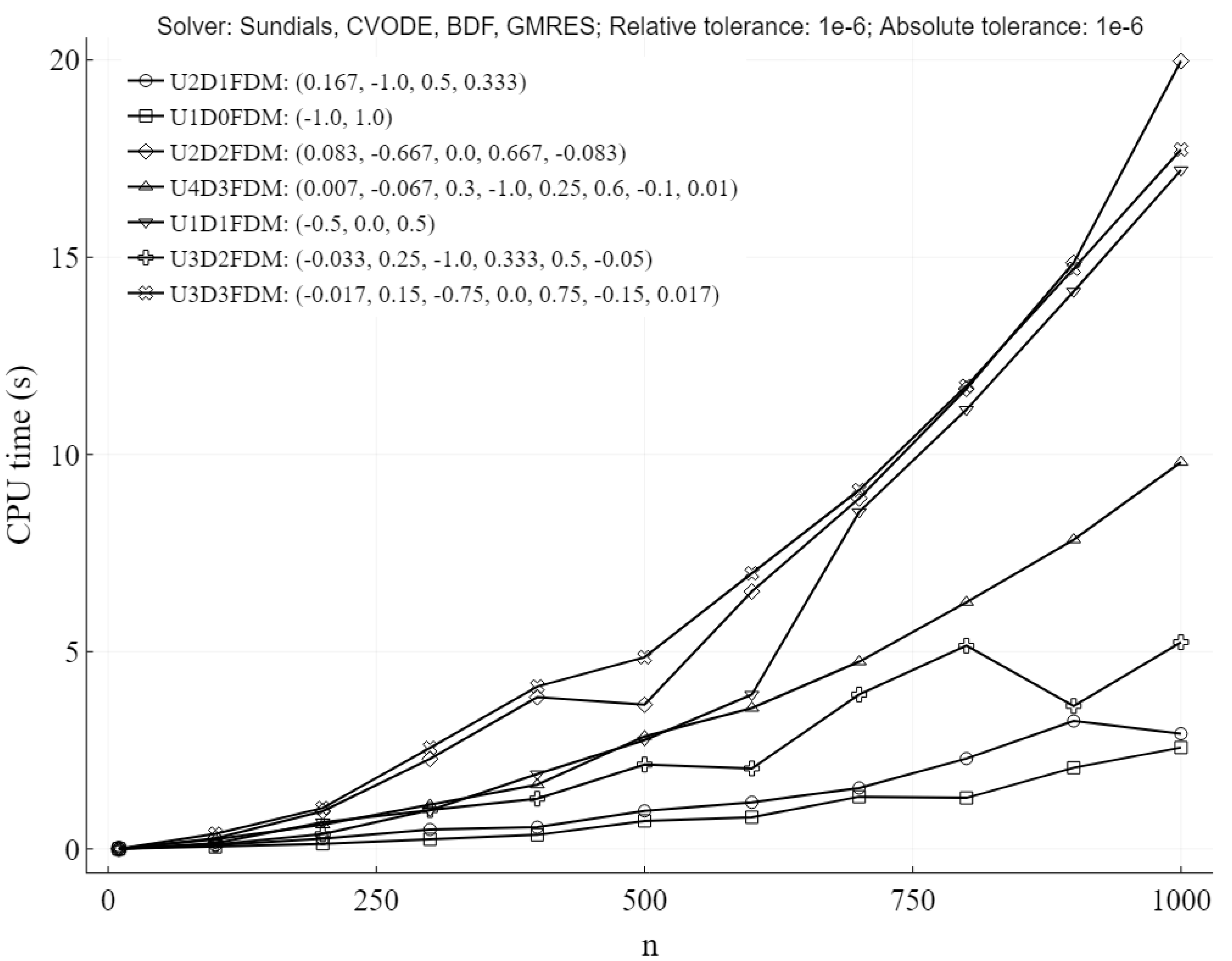
Figure 3.
Comparison of computational time of the tests between upwind-biased and central schemes for FDM. Similar results can be observed for FVM. The values in brackets represent rounded row stencil coefficients in the typical row of the derivative operator A (when Δx = 1).
Figure 3.
Comparison of computational time of the tests between upwind-biased and central schemes for FDM. Similar results can be observed for FVM. The values in brackets represent rounded row stencil coefficients in the typical row of the derivative operator A (when Δx = 1).

Figure 4.
Examples of well-behaving advection schemes. (a): Higher order upwind biased FVM scheme with mild numerical diffusion and mild oscillations; (b): Higher order upwind biased FDM scheme with mild numerical diffusion and very mild oscillations.
Figure 4.
Examples of well-behaving advection schemes. (a): Higher order upwind biased FVM scheme with mild numerical diffusion and mild oscillations; (b): Higher order upwind biased FDM scheme with mild numerical diffusion and very mild oscillations.

Figure 5.
Effect of physical diffusion on unphysical oscillation on sharp interfaces for na = 100 (the critical Peclét number, which makes the residual oscillation less than 10−6. It is approximately 6.47 for the U2D1FVM and 8.51 for the U2D1FDM).
Figure 5.
Effect of physical diffusion on unphysical oscillation on sharp interfaces for na = 100 (the critical Peclét number, which makes the residual oscillation less than 10−6. It is approximately 6.47 for the U2D1FVM and 8.51 for the U2D1FDM).

Figure 6.
Graphical representation of the variables.

Figure 7.
Demonstration of the solution quality (in the radial model) at 10 s for different subdivisions (Case 1).
Figure 7.
Demonstration of the solution quality (in the radial model) at 10 s for different subdivisions (Case 1).

Figure 8.
Absolute maximum temperature error estimations of the inner wall surface (Case 1).

Figure 9.
Absolute maximum temperature error estimations of the outer surface (Case 1).

Figure 10.
Relative maximum temperature error estimations of the inner surface (Case 1).

Figure 11.
Relative maximum temperature error estimations of the outer surface (Case 1).

Figure 12.
Absolute maximum temperature error estimations of the inner surface (Case 2).

Figure 13.
Absolute maximum temperature error estimations of the outer surface (Case 2).

Figure 14.
Relative maximum temperature error estimations of the inner surface (Case 2).

Figure 15.
Relative maximum temperature error estimations of the outer surface (Case 2).

Figure 16.
Estimations of maximal absolute errors at the outlet of the pipe (Case 1), where the red arrow signifies the ideal direction for discretization.
Figure 16.
Estimations of maximal absolute errors at the outlet of the pipe (Case 1), where the red arrow signifies the ideal direction for discretization.

Figure 17.
Estimations of maximal relative errors at the outlet of the pipe (Case 1), where the red arrow signifies the ideal direction for discretization.
Figure 17.
Estimations of maximal relative errors at the outlet of the pipe (Case 1), where the red arrow signifies the ideal direction for discretization.

Figure 18.
Computation times of the composite model tests (Case 1).

Figure 19.
Estimations of maximal absolute errors at the outlet of the pipe (Case 2), where the red arrow signifies the ideal direction for discretization.
Figure 19.
Estimations of maximal absolute errors at the outlet of the pipe (Case 2), where the red arrow signifies the ideal direction for discretization.

Figure 20.
Estimations of maximal relative errors at the outlet of the pipe (Case 2), where the red arrow signifies the ideal direction for discretization.
Figure 20.
Estimations of maximal relative errors at the outlet of the pipe (Case 2), where the red arrow signifies the ideal direction for discretization.

Figure 21.
Computation times of the composite model tests (Case 2).

Figure 22.
Comparison of Case 1 and Case 2 (with constant mass flow of 282.74 kg/s).

Figure 23.
Comparison with a model from Fluent (the solid material property differ slightly here—mass density is 7850 kg/m3, heat conductivity is 50 W/(mK), and specific heat capacity is 500 J/(kgK)).
Figure 23.
Comparison with a model from Fluent (the solid material property differ slightly here—mass density is 7850 kg/m3, heat conductivity is 50 W/(mK), and specific heat capacity is 500 J/(kgK)).

Figure 24.
Detail of the difference in temperature on comparison with a model from Fluent.

Figure 25.
Comparison with a model from STAR-CCM+.

Figure 26.
Detail of the difference in temperature on comparison with a model from STAR-CCM+.

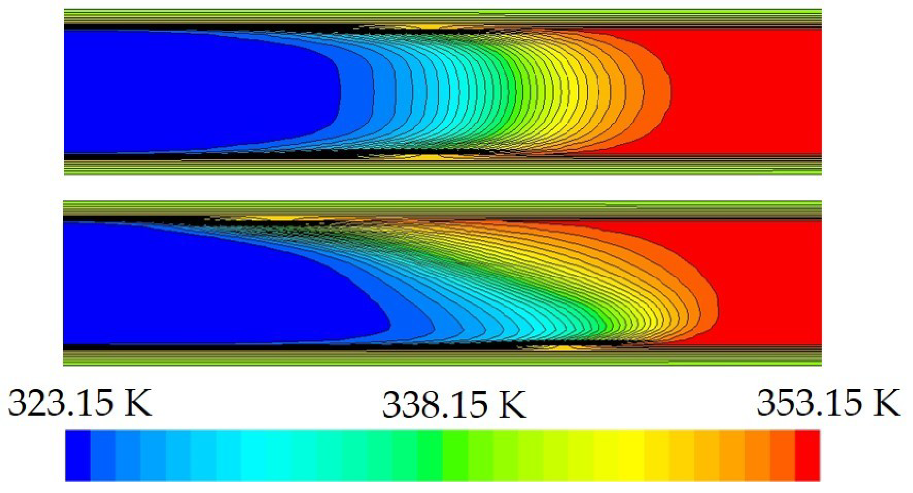
Figure 27.
Effect of gravity on the temperature distribution of a hot wave (the upper part shows the temperature front without effects of gravity, the lower part shows the contrary).
Figure 27.
Effect of gravity on the temperature distribution of a hot wave (the upper part shows the temperature front without effects of gravity, the lower part shows the contrary).

Figure 28.
Effect of gravity on the temperature distribution of cold wave (the upper picture shows the temperature front without effects of gravity, the lower picture shows the contrary).
Figure 28.
Effect of gravity on the temperature distribution of cold wave (the upper picture shows the temperature front without effects of gravity, the lower picture shows the contrary).


Table 1.
The property material of the steel circular wall (inner pipe diameter is 0.6 m).
| Property | Case 1 Accumulation | Case 2 No Accumulation |
|---|---|---|
| Layer thickness (mm) | 100 | 4 |
| Mass density (kg/m3) | 8030 | 8030 |
| Heat conductivity (W/mK) | 16.27 | 16.27 |
| Specific heat capacity (J/kgK) | 502.45 | 502.45 |
© 2019 by the authors. Licensee MDPI, Basel, Switzerland. This article is an open access article distributed under the terms and conditions of the Creative Commons Attribution (CC BY) license (http://creativecommons.org/licenses/by/4.0/).
Share and Cite
MDPI and ACS Style
Kudela, L.; Chylek, R.; Pospisil, J. Performant and Simple Numerical Modeling of District Heating Pipes with Heat Accumulation. Energies 2019, 12, 633. https://doi.org/10.3390/en12040633
AMA Style
Kudela L, Chylek R, Pospisil J. Performant and Simple Numerical Modeling of District Heating Pipes with Heat Accumulation. Energies. 2019; 12(4):633. https://doi.org/10.3390/en12040633
Chicago/Turabian StyleKudela, Libor, Radomir Chylek, and Jiri Pospisil. 2019. "Performant and Simple Numerical Modeling of District Heating Pipes with Heat Accumulation" Energies 12, no. 4: 633. https://doi.org/10.3390/en12040633
Note that from the first issue of 2016, this journal uses article numbers instead of page numbers. See further details here.