Optimal Multidimensional Droop Control for Wind Resources in DC Microgrids

1
Department of Electrical & Computer Engineering, Michigan Technological University, Houghton, MI 49931, USA
2
Rocky Mountain Institute, Boulder, CO 80302, USA
*
Author to whom correspondence should be addressed.
Energies 2018, 11(7), 1818; https://doi.org/10.3390/en11071818
Submission received: 11 June 2018
/
Revised: 29 June 2018
/
Accepted: 10 July 2018
/
Published: 11 July 2018
Abstract
:The inclusion of electricity generation from wind in microgrids presents an important opportunity in modern electric power systems. Various control strategies can be pursued for wind resources connected in microgrids, and droop control is a promising option since communication between microgrid components is not required. Traditional droop control does have the drawback of not allowing much or all of the available wind power to be utilized in the microgrid. This paper presents a novel droop control strategy, modifying the traditional approach and building an optimal droop surface at a higher dimension. A method for determining the optimal droop control surface in multiple dimensions to meet a given objective is presented. Simulation and hardware-in-the-loop experiments of a sample microgrid show that much more wind power can be utilized, while maintaining the system’s bus voltage and still avoiding the need for communication between the various components.
1. Introduction
Two emerging technologies that are important in the modern electric power system include wind turbines and microgrids. The use of wind to generate electricity has become increasingly common and provides a clean, sustainable source of energy. Microgrids are small electricity systems that can operate in connection with the main power grid, but are also able to operate in a disconnected or islanded mode. They allow for a more reliable and efficient power system, since electricity does not have to be transmitted long distances to reach customers [1].
Including wind turbines as part of the generation mix in a microgrid is one way to take advantage of the benefits of both of these technologies [2]. The size of both wind turbines and microgrids can vary greatly. In this paper, an example microgrid is presented that could represent a small building, with one wind turbine and one liquid-fuel generator. An updated droop control scheme is presented for wind turbines connected with microgrids, which allows more of the power available from the wind to be utilized.
Droop control is a common control method for power systems, including DC [3] and islanded [4] microgrids. The main benefit of droop control is that sources and loads are not required to communicate or share information with one another [5]. In a DC distribution system, each source is assigned a droop setting so that the power supplied by each source changes as the system load changes. All of the microgrid components are connected to a common bus, so fluctuations in the load cause fluctuations in the bus voltage. The nominal bus voltage is always the same for all sources, but assigning different droop settings allows each source to supply more or less power as the bus voltage changes [5].
The application of droop control has been studied with microgrids and specifically with microgrids containing wind resources. Researchers have proposed various adjustments to traditional droop control, to achieve improved operation when applied with wind resources and with microgrids. For example, Luo et al. proposed an offset in addition to the linear droop setting for sources connected to the DC microgrid bus [6]. Additional research has suggested increasing droop gains in a DC microgrid as the load level increases to improve current sharing among sources [7].
In one study of the application of droop control with wind resources in microgrids, two distinct droop settings were recommended: one for operation in connection with the larger grid and one for operation in islanded mode [8]. Another approach giving lower droop settings to those sources with higher power margins was proposed [9], in order to improve frequency regulation of wind turbines. The implementation of droop control with wind sources in microgrids was also shown in [10].
Successful implementation of droop control with wind sources in a standalone DC microgrid has been demonstrated [11]. For an AC microgrid, previous research has suggested including control to improve the performance of traditional droop control and reduce errors based on measurement noise [12].
The challenges encountered in using droop control with wind resources due to the variable nature of wind are clear [13]. When using traditional linear droop control, appropriate droop control settings that allow for load sharing while also utilizing energy from the wind are difficult to find. This paper will present an alternative droop control method to address these challenges. Another common type of control for wind resources in Maximum Power Point Tracking (MPPT); this paper presents an alternative approach using a modified droop control method.
Unlike diesel or other fossil fuel-based generators, wind generation includes uncertainties due to the variable nature of the power available with changing wind conditions. Optimization of the number and location of distributed wind generators given these uncertainties has been demonstrated [14], and the droop control method proposed here is designed to optimize the utilization of wind resources given the uncertainties in their operation over time.
One application for this research is remote microgrids, which are not located near the main electrical grid and therefore operate as standalone systems. These microgrids may also be located in countries that do not have a centralized electricity grid system or on physical island communities [15]. In some cases, these communities have relied on diesel generation; the addition of renewable energy resources with control methods such as droop control can reduce their consumption of diesel fuel, leading to reduced operational costs and reduced carbon emissions [16].
Alternatively, some microgrids have the option to operate while connected with the grid, or in a separate, islanded mode [17]. The improved droop control method proposed in this paper can be applied with a microgrid that is operating as an island. Stability is important regardless of the operational mode, but becomes especially important in islanded microgrids [18].
Previous work has demonstrated the use of multidimensional droop control with wind resources, where a plane is used for the droop control relationship rather than the traditional line [19]. Related work has presented a method for finding an optimal droop control relationship in two dimensions to meet a given objective [20]. This paper presents an improved method for designing droop control for wind resources in DC microgrids, combining each of these two approaches to create an optimal multidimensional droop controller.
2. Microgrid Modeling and Control
A simplified modeling approach will be used for DC sources connected through a power electronics converter to the microgrid and controlled using droop control. This equivalent approach allows the converter model to be simplified to only a variable output voltage, without including the actual switching, or an average model of the switching, in the simulation. This approach will be used in this paper as a preliminary method for modeling the system and designing droop control algorithms. Average mode modeling for power electronics will then be simulated [21], and full switching models will be implemented using hardware-in-the-loop.
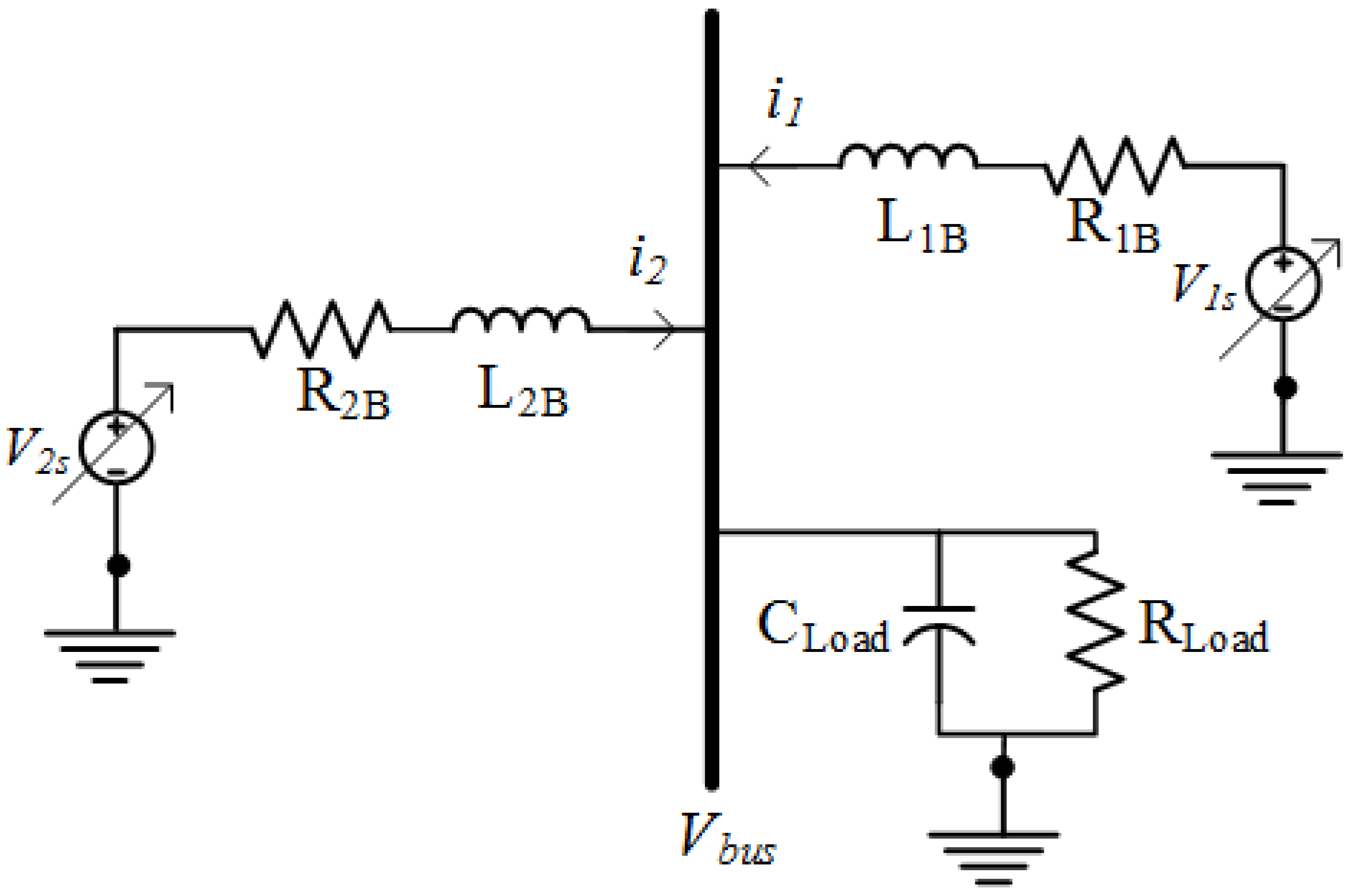
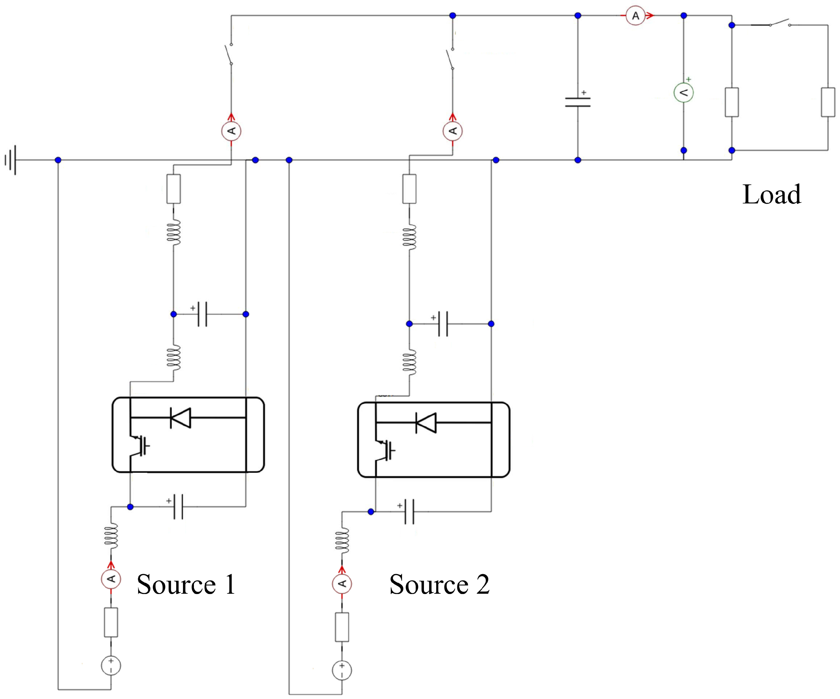
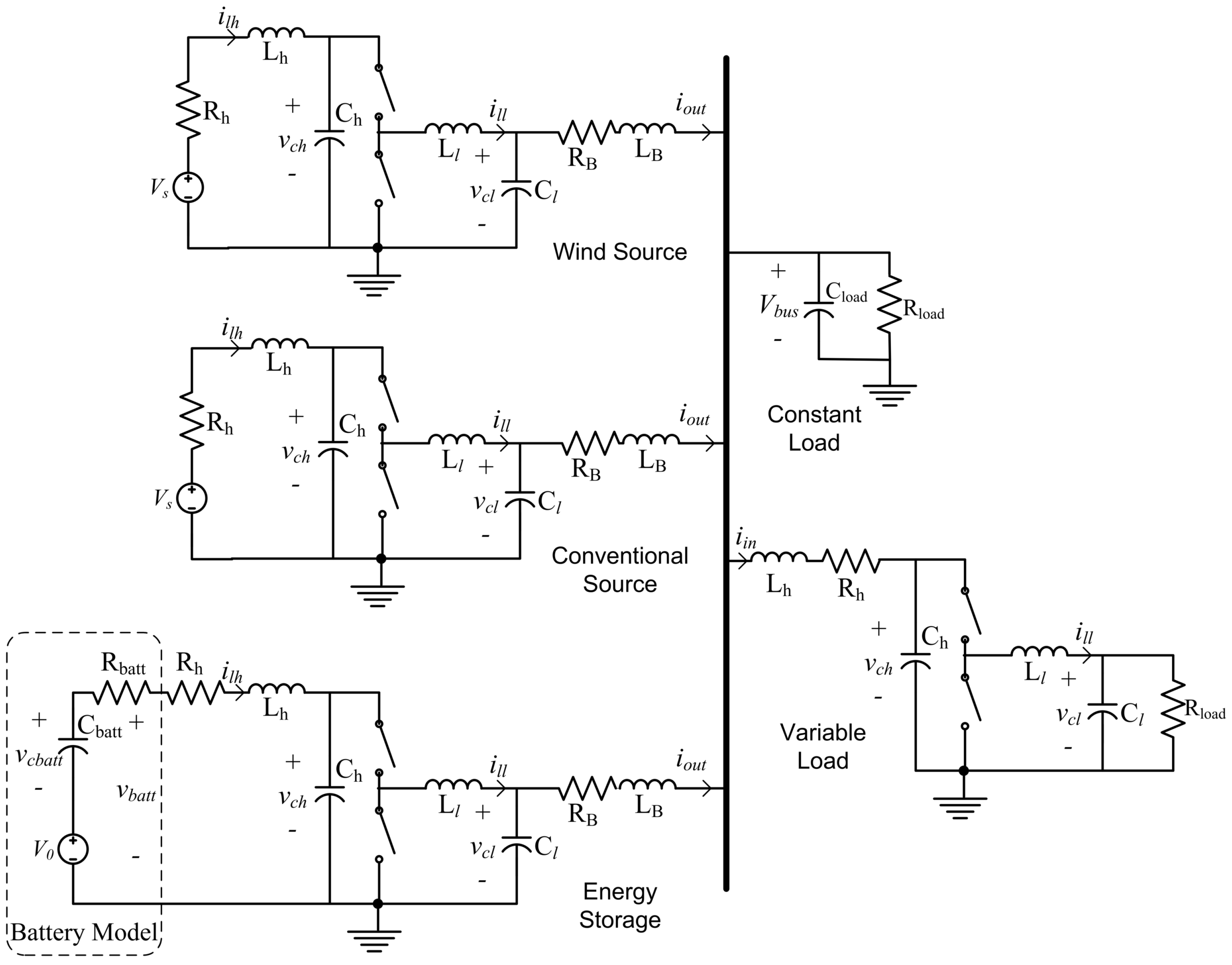
The example microgrid system used in the first part of this paper is shown in Figure 1. Five state equations define this system: one for the bus voltage, one for the droop controller for each source and one for the current from each source.
Source voltages and can then be replaced by implementing proportional-integral control loops as:
Source 2 will utilize traditional linear droop control, where:
The reference current for Source 1 is left as a variable, . The following section will demonstrate a method to find the optimal as a function of bus voltage and other variables to meet a given objective. The numeric values used for this microgrid model are shown in Table 1. The full state model and proportional-integral control design are presented in [19].
Optimization of Droop Control
Using the system model defined above, this section will describe a method to identify an optimal droop control relationship between reference current, bus voltage and other variables to meet a given objective [20]. The state equation model of the system is first solved to find the steady-state result, since droop control allows a system to move between stable steady-state points [5].
Most of the quantities in this steady-state result are constant system parameters or control values that will be selected. The load resistance is the only remaining item that can vary. Since we are solving for as a function of , the steady-state result can be used to solve for the load resistance:
The power supplied by Source 1 in steady state can then be calculated, (14) used to replace and the result simplified to:
Given the steady-state power as a function of and , an objective function can be selected, and we can solve for as a function of that meets that objective in an optimal way. For example, choose an objective to have a constant output power from Source 1, regardless of changes in the system load,
where is the desired power for Source 1 to supply. The full objective function is then:
Taking the derivative of the objective function with respect to and setting the result equal to zero results in:
Solving for the optimal gives the optimal relationship for reference current with respect to bus voltage, desired output power and line resistance,
Previous work implemented a constant desired power of 2000 W and demonstrated the operation of the microgrid using this optimal droop control relationship in two dimensions [20]. If the desired power depends on an additional variable, it becomes , where w is the wind speed, for example. The optimal droop control relationship is now a function in multiple dimensions:
The use of this control strategy is demonstrated in the following sections.
3. Small Microgrid
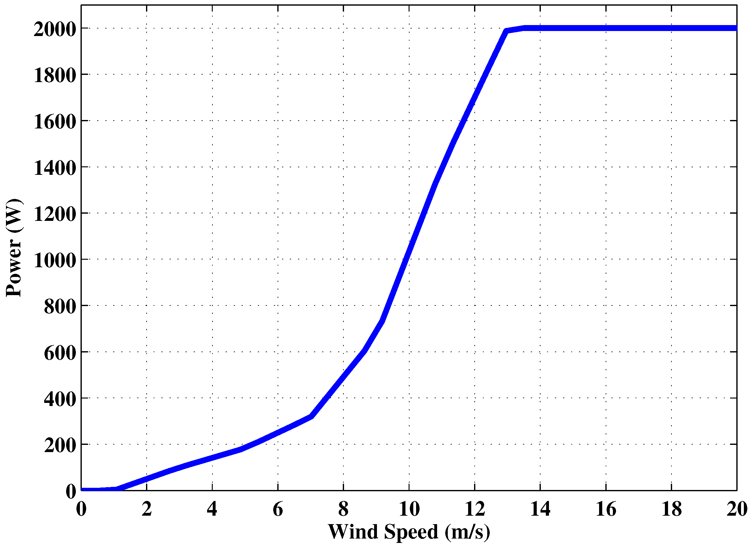
As an initial example, the small microgrid shown in Figure 1 is used. For this example, a 2-kW wind turbine is simulated. The power curve for the turbine is shown in Figure 2; this relationship is used to replace in (20). Source 2 represents a small diesel generator.
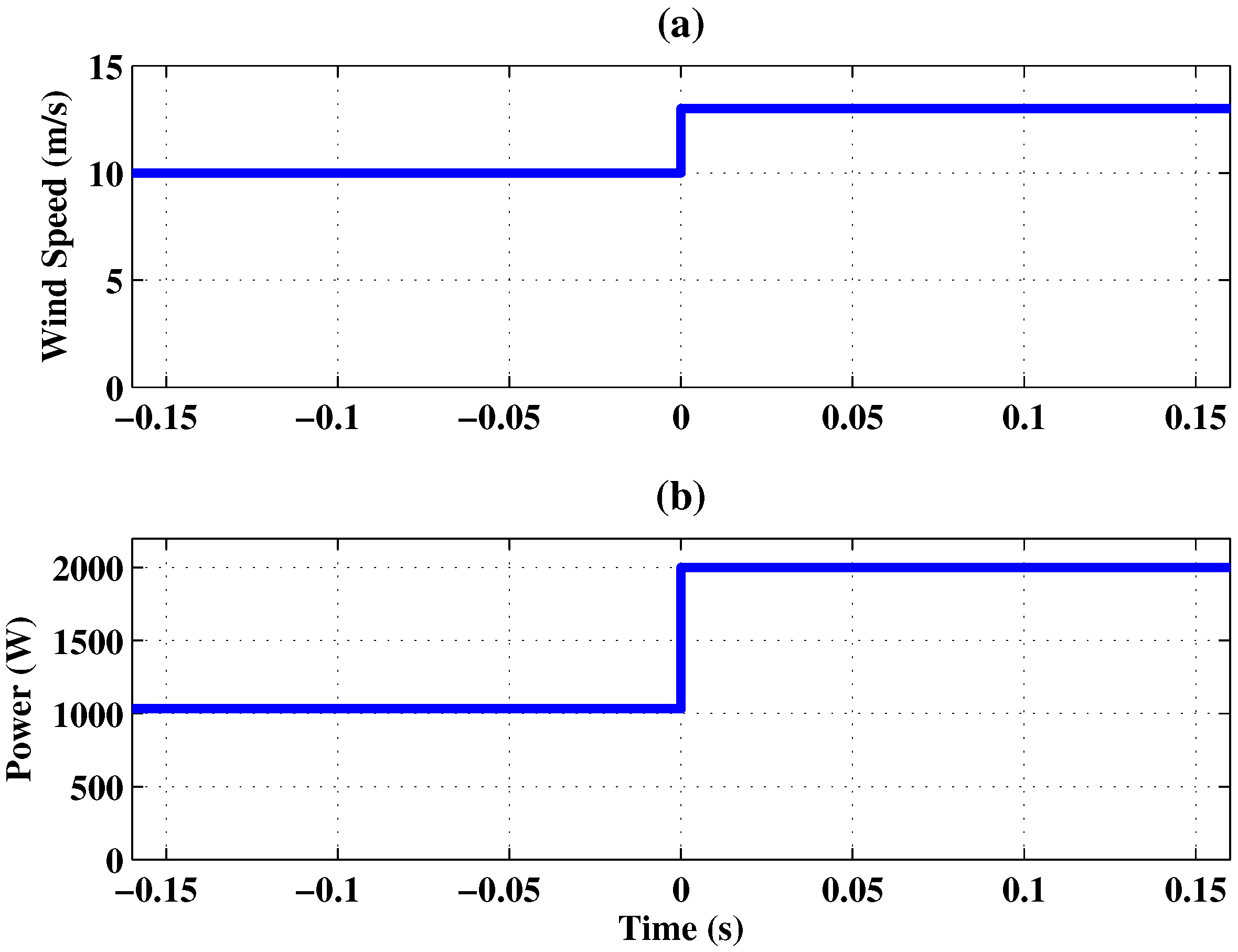
For a first test case, a step change in wind speed from 10 m/s–13 m/s was implemented first in simulation and then hardware-in-the-loop. Figure 3 shows this step change in wind speed, along with the associated step change in power available from the wind, based on Figure 2.
3.1. Simulation Results
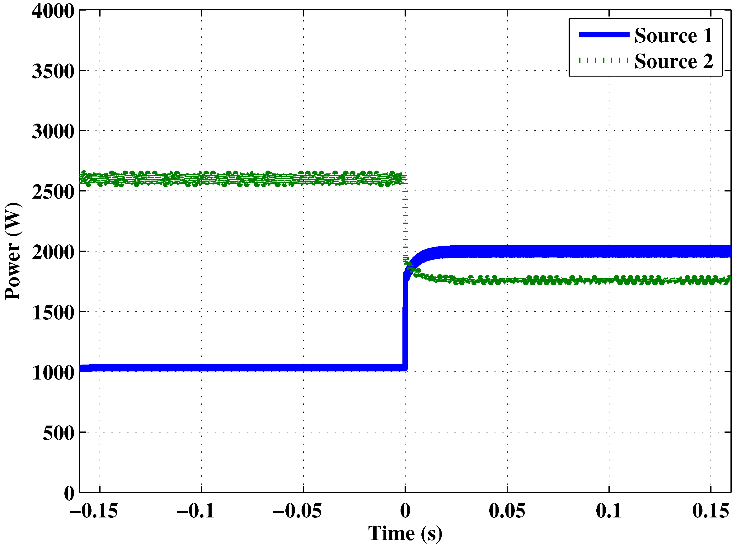
The system was simulated using the optimal multidimensional droop control relationship found in (20). Figure 4 shows the power supplied by each source during the simulation. When the wind speed is increased at , the power supplied by Source 1 increases to match the new level of available power from the wind.
3.2. Hardware-In-The-Loop Results
A Hardware-In-the-Loop (HIL) approach was used to verify the simulation results presented in the previous section. This allows the system to be emulated in software, while connecting with real-world hardware in real time [22]. Using an HIL approach allows the proposed control method to be tested virtually with an example system, while interfacing with real hardware [23].
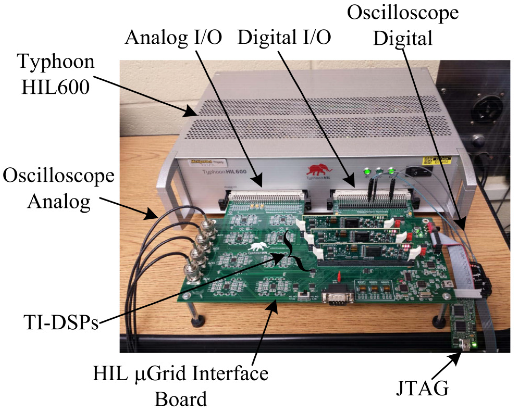
Both the simulation and HIL used the same component values; the HIL experimental apparatus is shown in Figure 5. This particular HIL unit, the Typhoon HIL600, has 32 channels of ±5-V Analog Output (AO) that are mapped to data points in the HIL circuit. These signals are then offset and scaled by the microgrid control board to 0 V–+3.3 V and are read by the 12-bit analog to digital converters on three DSPs. For this test, five channels of analog signals are needed to implement the multidimensional optimal droop control. The analog signal parameters and the scaling from the HIL are shown in Table 2.
BNC connectors on the microgrid control board are linked with the first four analog output channels that are then connected to an oscilloscope. For this research, the first three channels are used to view , and and capture the results in oscilloscope traces.
The droop controller for each source was implemented on an individual Texas Instruments F28335 DSP ControlCARD [24]; each was then programmed through the Embedded Coder toolbox in MATLAB/Simulink (Verison 2014b, Mathworks, Natick, MA, USA). The control card for Source 1 implements optimal multidimensional droop control as in (20), while the card for Source 2 implements linear droop control as in (8), each using a PID control loop. Using separate control cards for each of the two sources ensures the implementation of decentralized control; each source uses only local information, and communication between sources and/or the other microgrid components is not required.
For the HIL experiment, all power electronics switching was included, along with parasitic inductances and capacitances. The circuit schematic used in the Typhoon software is shown in Figure 6. The parameter values used for the two sources are shown in Table 3.
The optimal multidimensional droop control relationship in (20) was implemented in hardware-in-the-loop, and the same step change in wind speed that was used in the simulation was also used here.
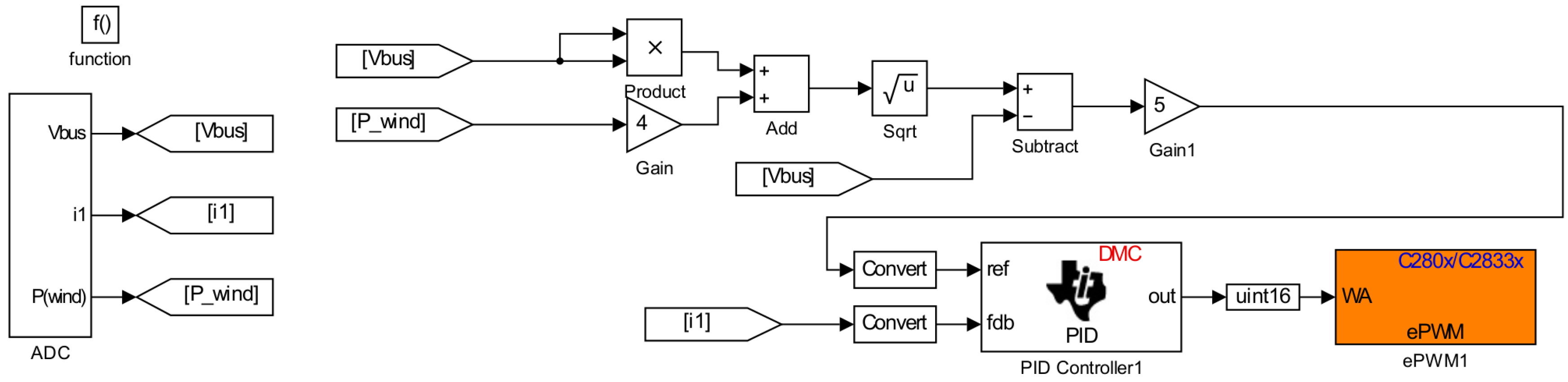
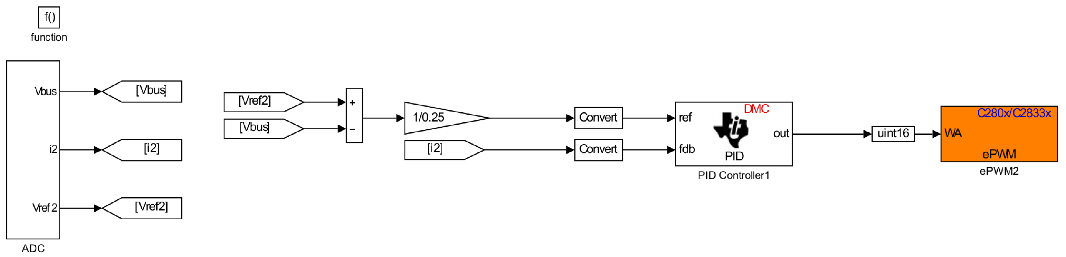
The optimal droop controller implemented for Source 1 is shown in Figure 7, while the traditional droop controller implemented for Source 2 is shown in Figure 8.
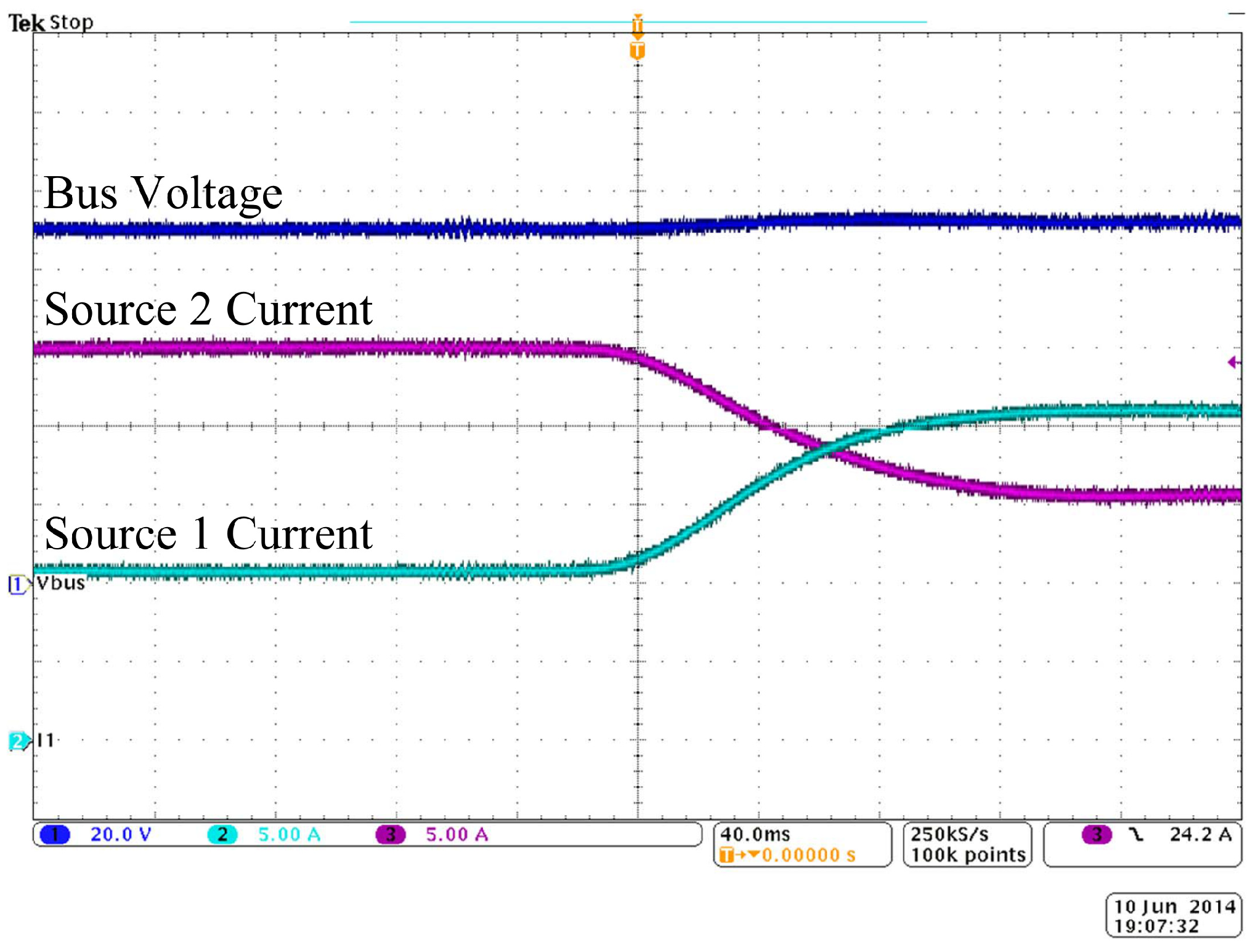
Figure 9 shows the microgrid bus voltage and the currents supplied by both sources. Both currents share the same zero point on the oscilloscope trace, while the bus voltage zero point is offset for visibility. As in the simulation results, when a step increase in the wind speed occurs, Source 1 increases its output based on the increased power available from the wind. Source 2 decreases its output so that the two sources together share the load, which is constant for this example.
3.3. Comparison of Results
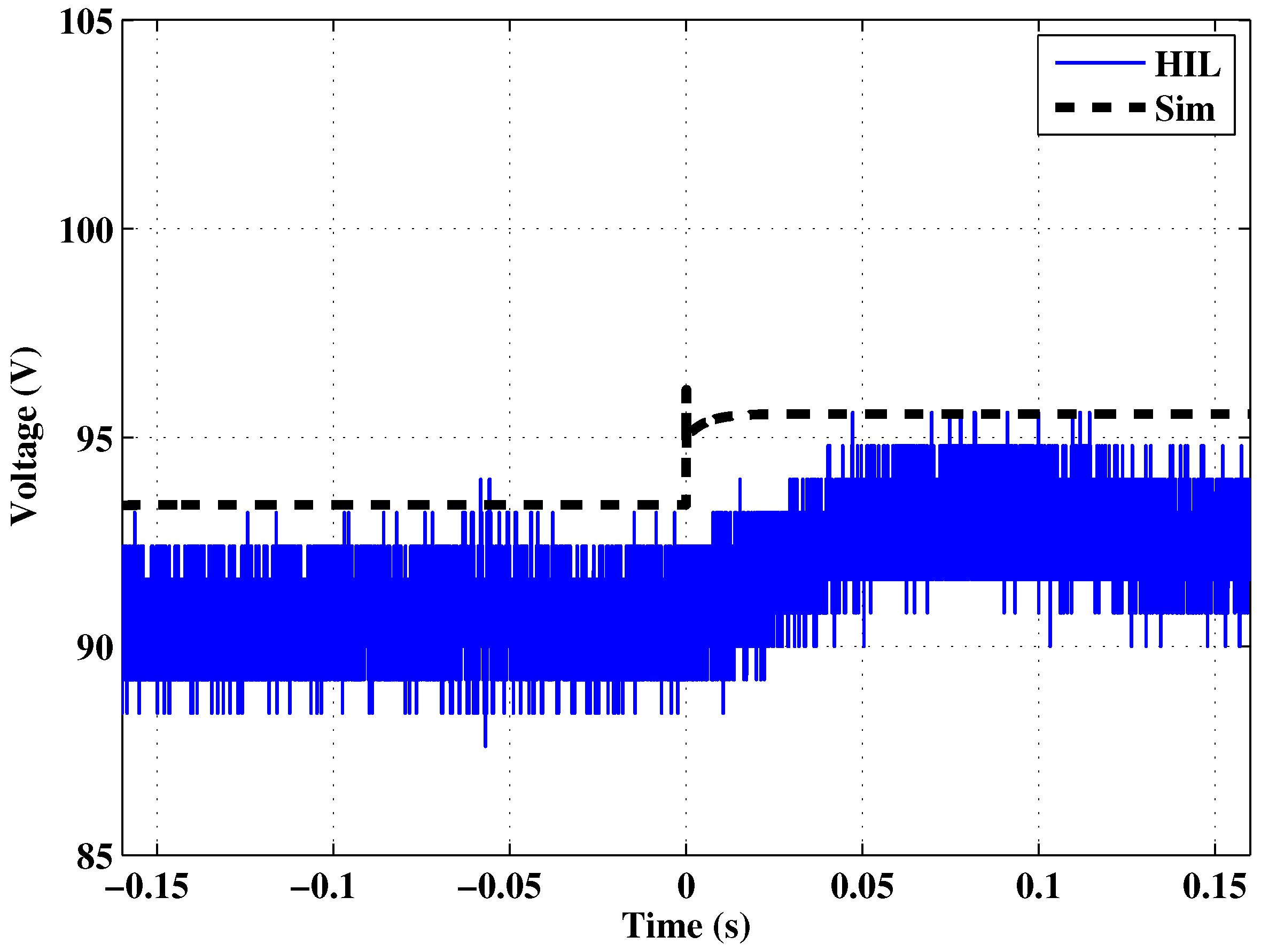
MATLAB was used to plot the imported data from the oscilloscope traces in Figure 9, along with the simulation results presented earlier. This demonstrates a direct comparison for the same scenario that was both simulated and tested using HIL. Figure 10 shows the microgrid bus voltage during the step change in wind speed, with both the simulation and HIL results shown together.
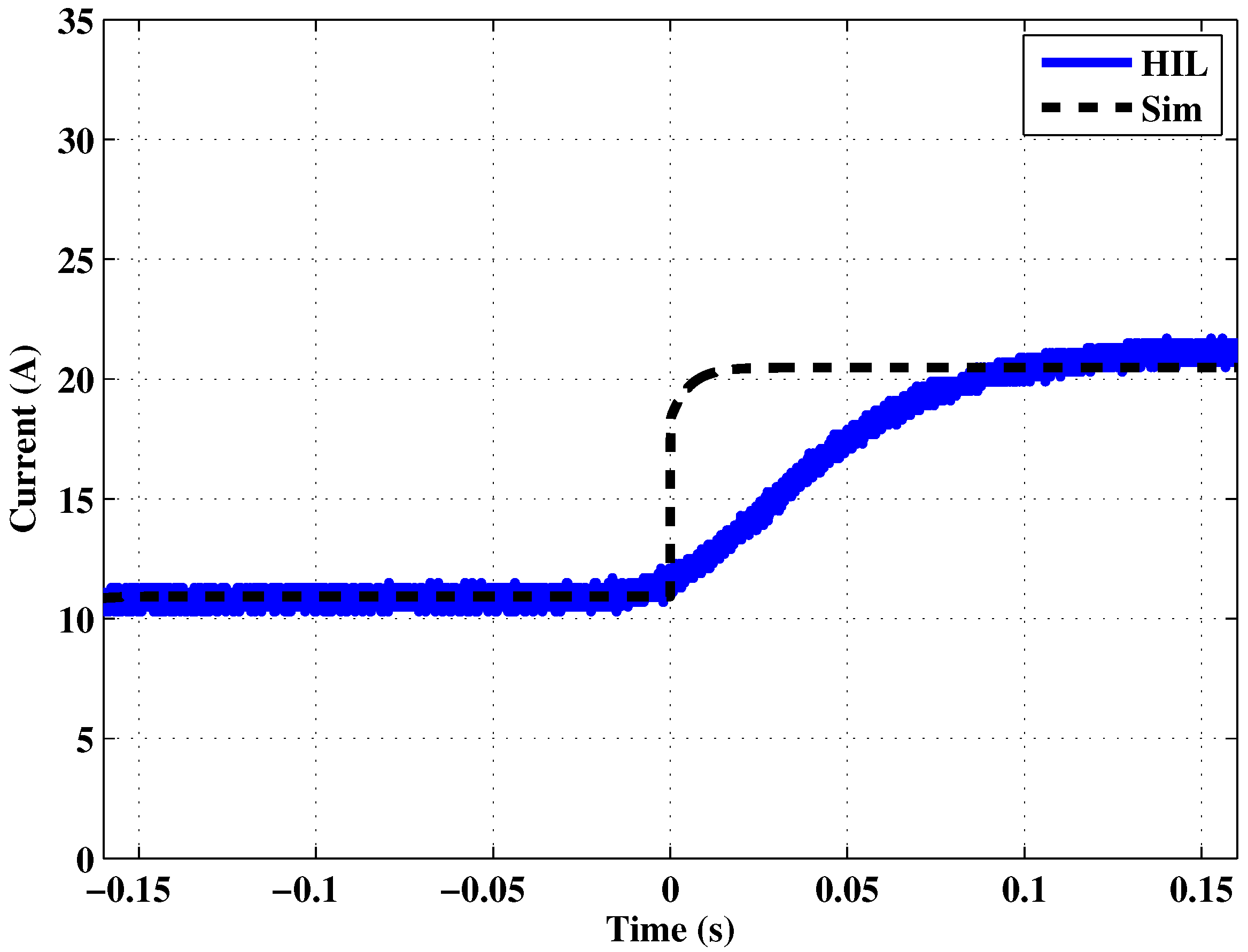
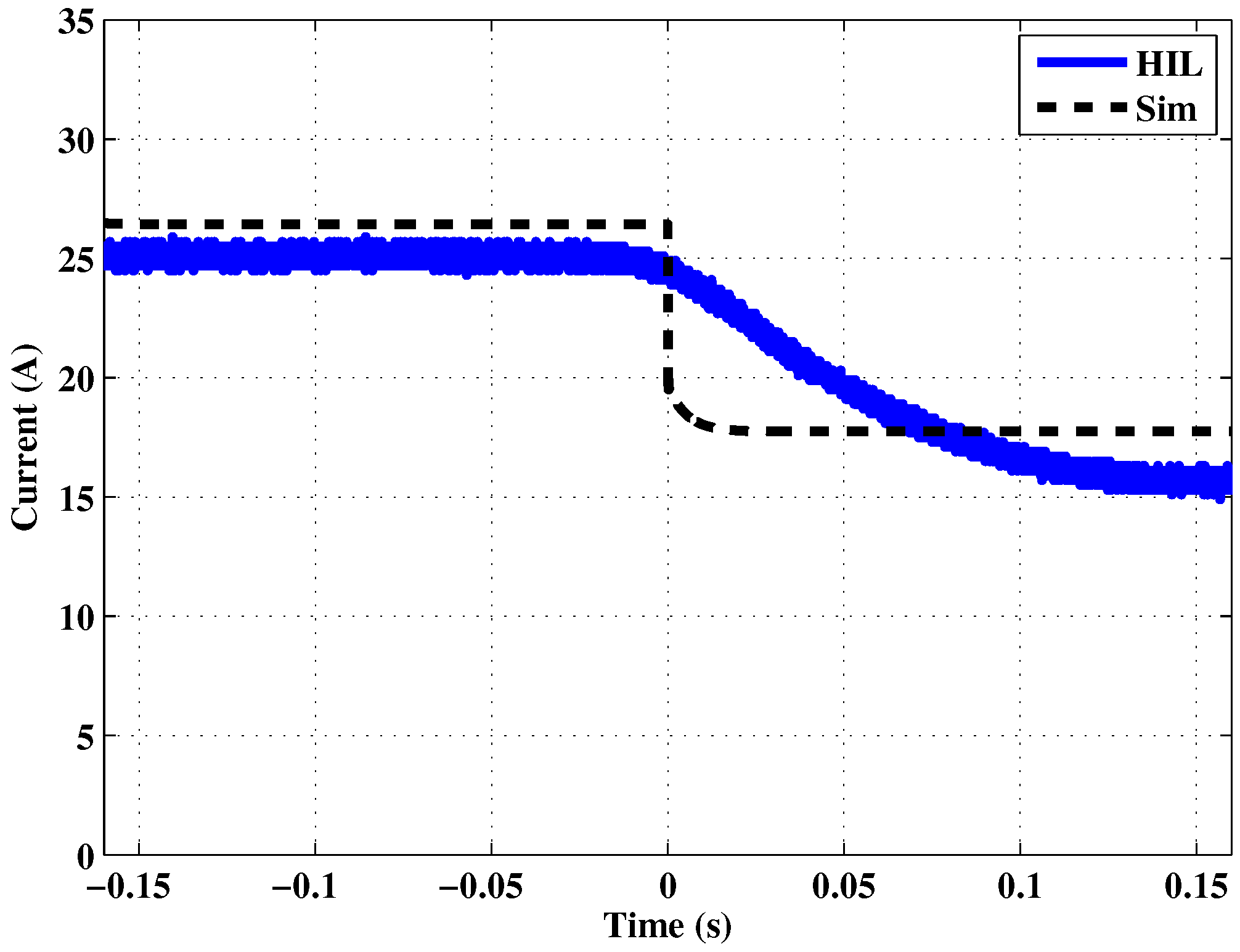
Figure 11 and Figure 12 show the current supplied by each source, with both the simulation and HIL results shown together. The simulation and HIL steady-state values of current before and after the step change in wind speed match; however, the two sets of results do not match during the transient event. This is due to the fact that different time constants were used in the simulation and HIL experiments. The proportional and integral gains for the PI controller in the simulation and HIL were also not tuned to achieve a very fast transient response. Since the control methods proposed in this paper are designed for use over large time periods, the difference found between simulation and HIL results for this test of a very small time period was not a key concern for this research.
4. Residential Microgrid
The simulation and HIL results presented above demonstrate the function of the proposed optimal multidimensional droop control method, using a small example microgrid with a constant load and a simple step change in wind speed. This section will compare the use of linear, planar and optimal multidimensional droop control with an example residential-scale microgrid. The details of the modeling method used for each component in the microgrid can be found in [19], and the full microgrid model is shown in Figure 13.
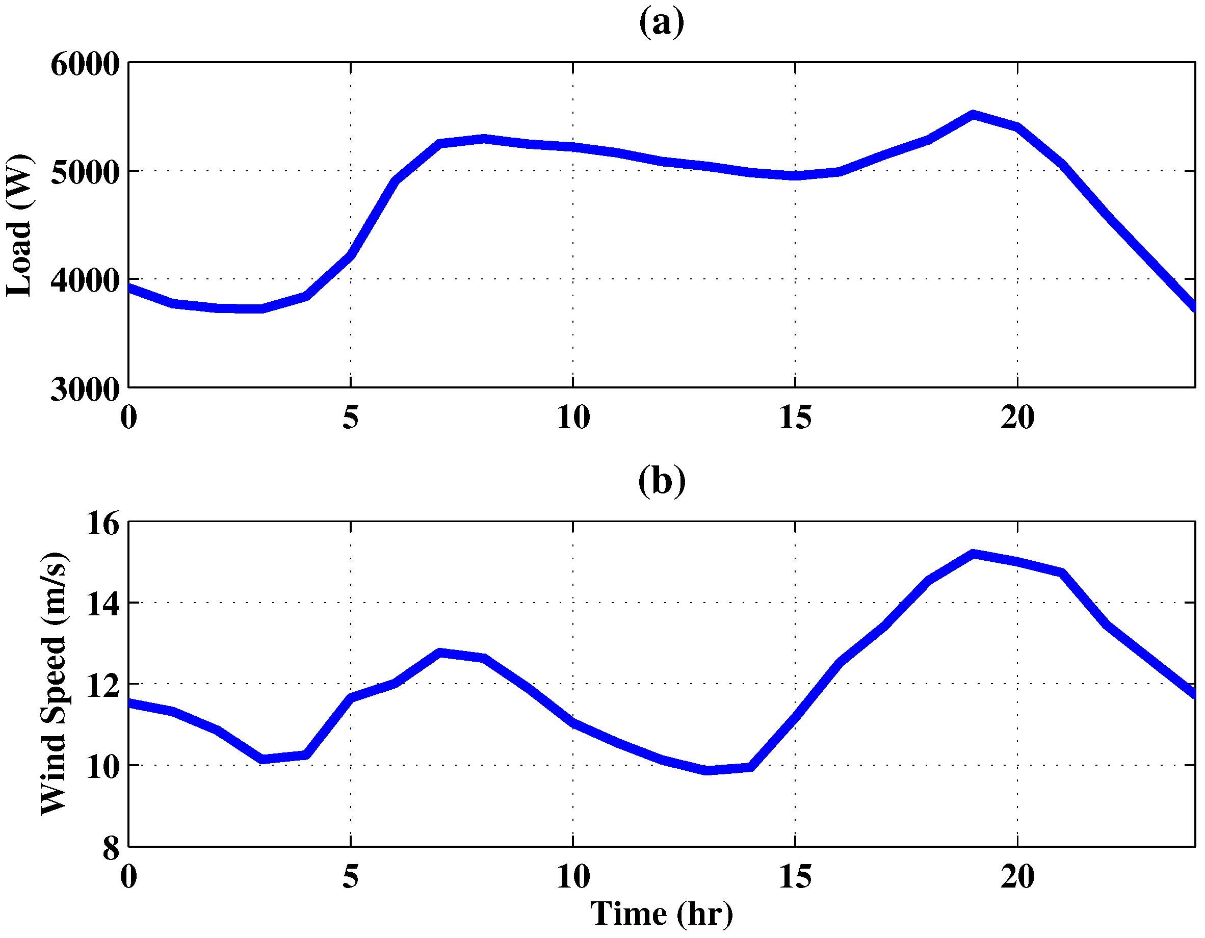
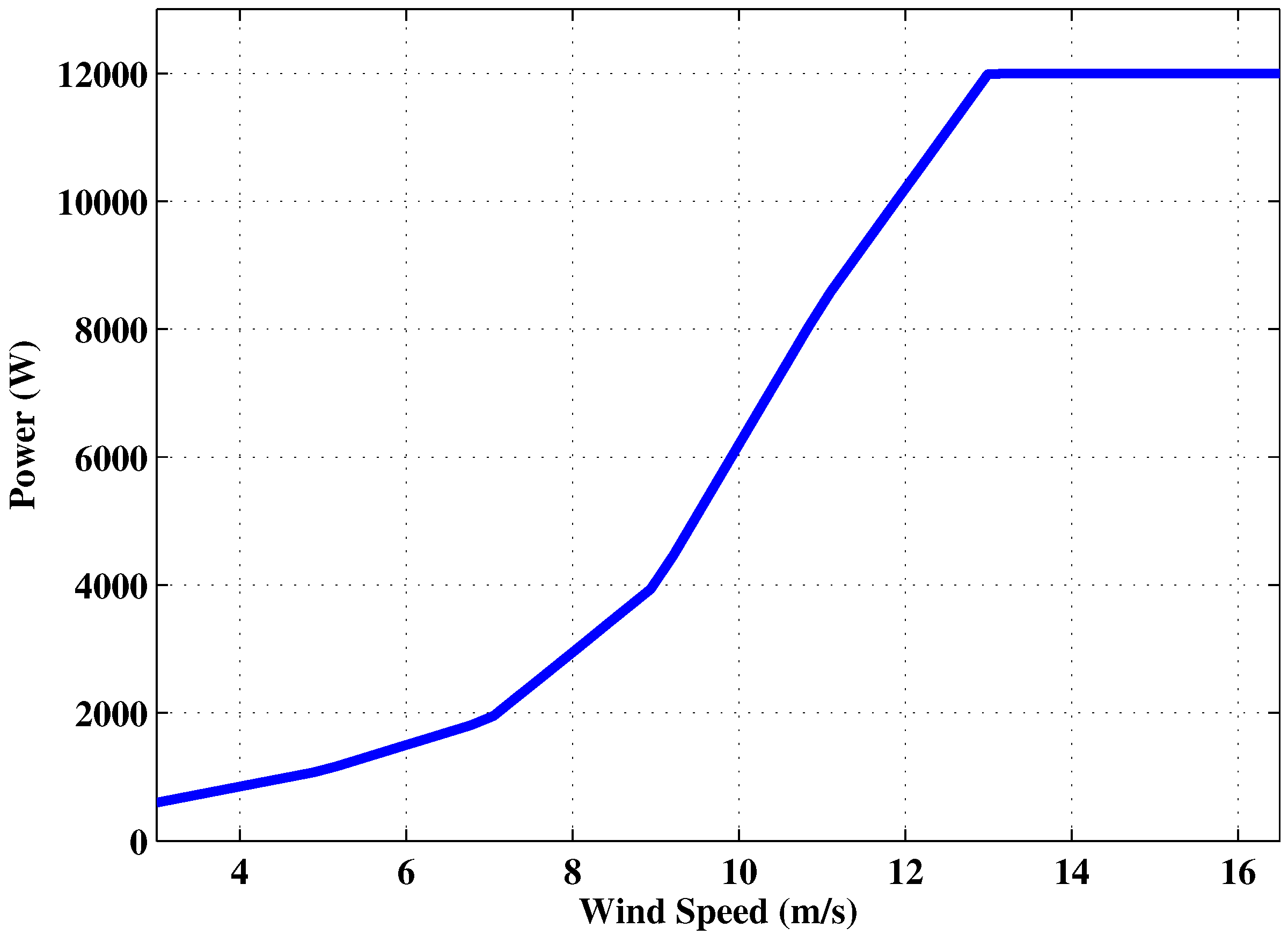
The full example microgrid was simulated three times: first with traditional linear droop control, then with multidimensional droop control using a plane and, finally, with optimal multidimensional droop control using a surface. The results using each type of control are presented in the following sections. The system was modeled for a 24-h period, using the wind speed and load profiles shown in Figure 14. A 12-kW wind turbine was simulated, with the power curve shown in Figure 15.
4.1. Traditional Droop Control
First, the system was simulated using traditional, linear droop control for both sources. The droop control relationships are shown in Figure 16. The conventional source and the energy storage device will keep their same linear droop control settings for all three of the simulations.
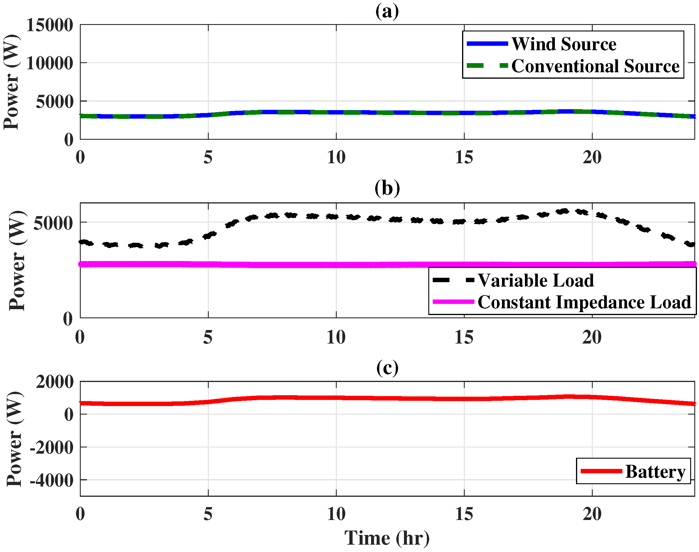
The results of simulating the system are shown in Figure 17. Both sources share the load, and the wind resource does not change its operation based on the wind speed. The battery is needed throughout the day to provide additional power to the system.
4.2. Multidimensional Droop Control
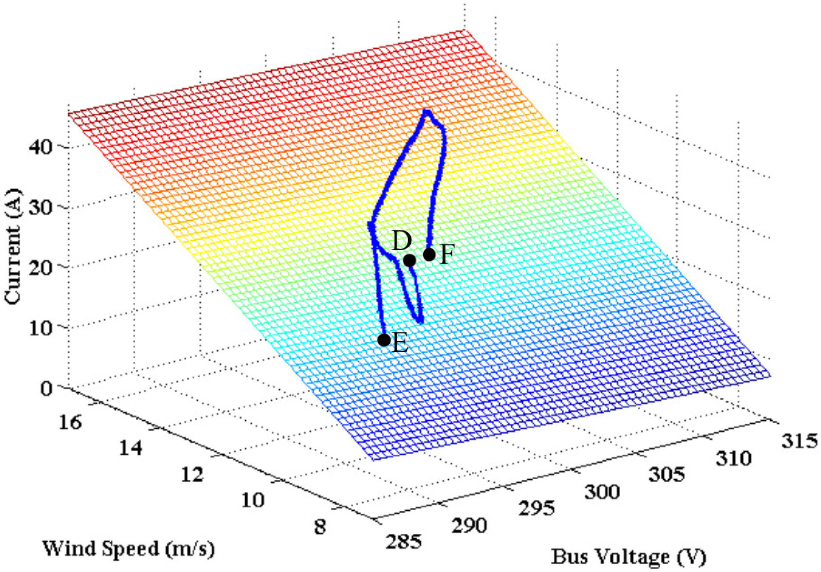
Next, the system was simulated using multidimensional droop control for the wind resource. The droop control plane is shown in Figure 18, along with the operation of the source during this simulation. The points marked D, E and F provide a reference for the plot of the source’s output with respect to time, which is shown in Figure 19.
The results of simulating the system are shown in Figure 19. The points marked D, E and F provide a reference to the source’s movement along the droop control plane, shown in Figure 18. Both sources share the load, and the wind resource changes its operation based on the wind speed. The conventional resource is needed during times of lower wind speed to ensure that the load is met. The battery is now able to charge during the times of higher wind speed.
4.3. Optimal Multidimensional Droop Control
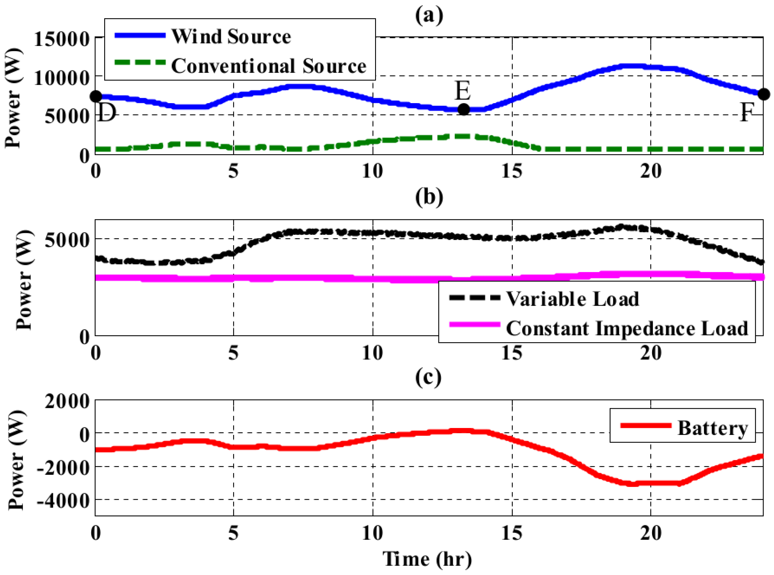
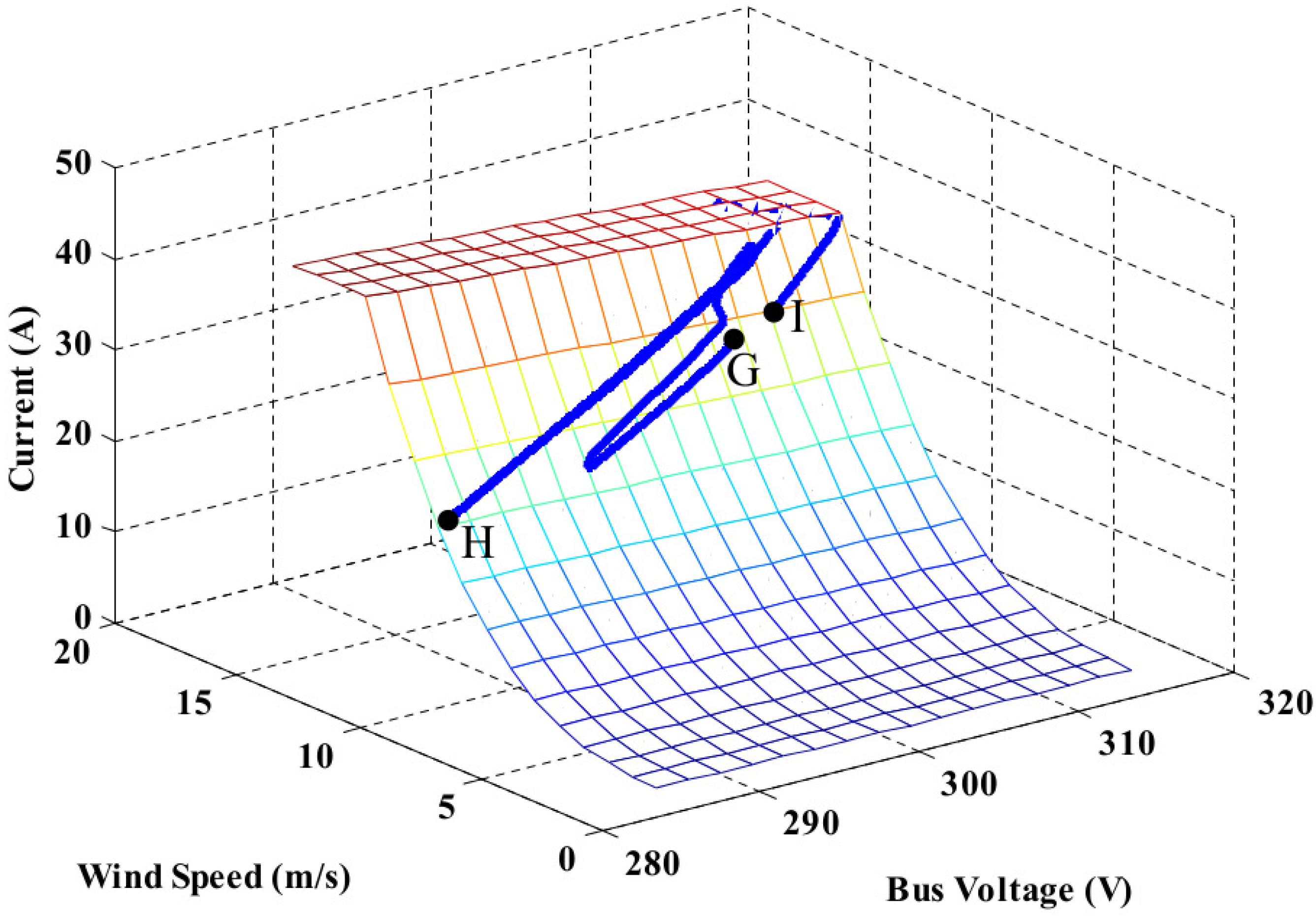
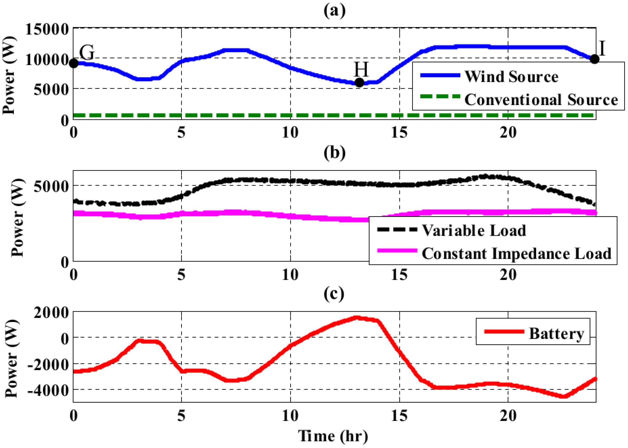
Finally, the system was simulated using optimal multidimensional droop control for the wind resource. The method presented above was used to find the optimal surface for a 12-kW wind turbine. The droop control surface is shown in Figure 20, along with the operation of the source during this simulation. The points marked G, H and I provide a reference for the plot of the source’s output with respect to time, which is shown in Figure 21.
The results of simulating the system are shown in Figure 21. The points marked G, H and I provide a reference to the plot of the source’s movement along the droop control surface, shown in Figure 20. Both sources share the load, and the wind resource changes its operation based on the wind speed. The conventional source outputs its minimum requirement of 500 W throughout the simulated day. The battery is able to charge for most of the day and supplies some power to the system when needed.
4.4. Comparison of Simulation Results
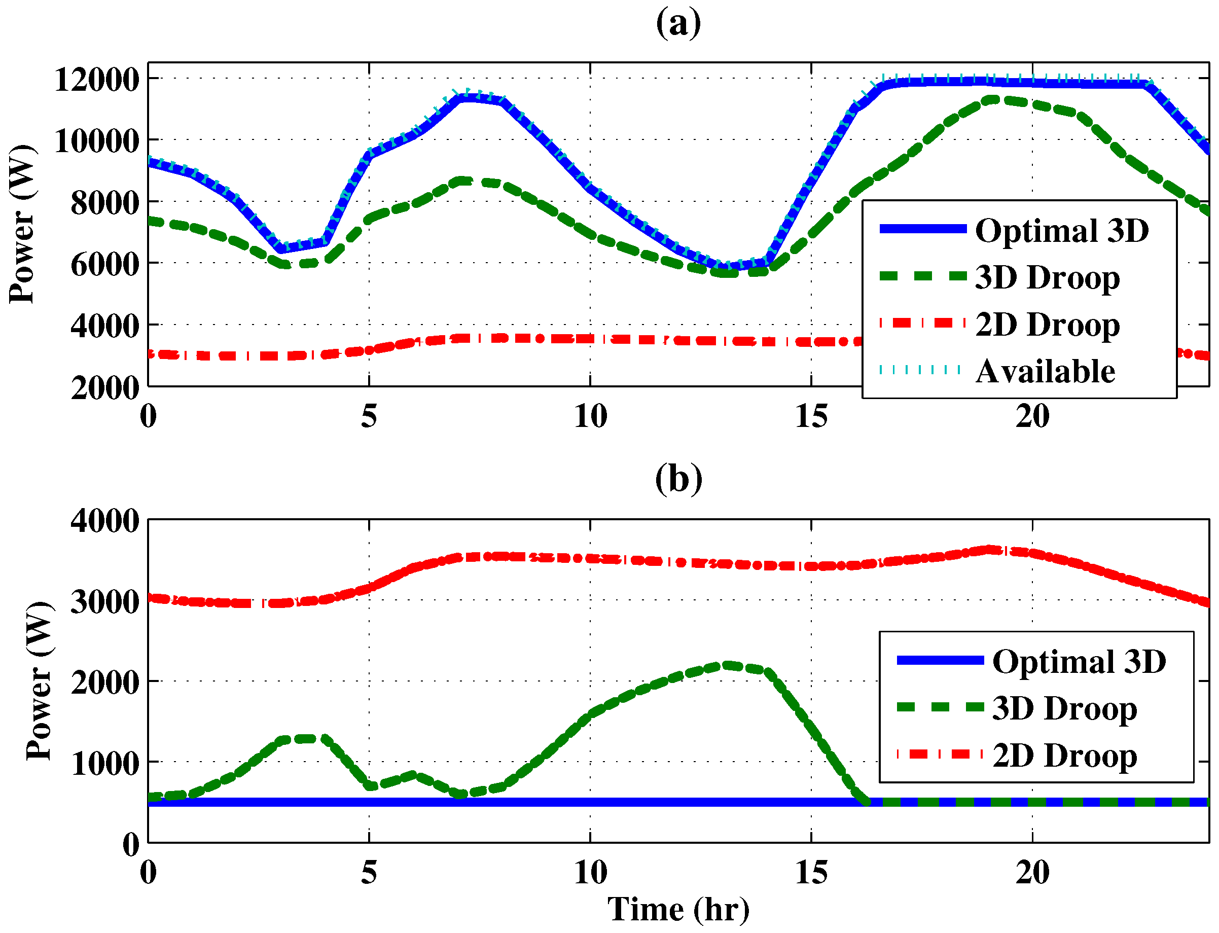
The power supplied from the two sources in each of the three simulations are compared in Figure 22. Using multidimensional droop control with a plane allows more of the energy from the wind to be utilized, while using an optimal multidimensional droop control surface allows almost all of it to be utilized. This also requires the conventional source to be used less, resulting in fuel savings.
A comparison of the amount of unused energy for each case is shown in Table 4. Using multidimensional droop control (a plane) decreases the unused energy by almost 75% compared to traditional linear droop control. Using the optimized droop surface for the wind source decreases the unused energy by an additional 94%.
The bus voltage during each of the simulations is shown in Figure 23. When multidimensional droop control is used, with both a plane and an optimal surface, the bus voltage varies more than in the traditional linear droop control case. This is one trade-off that needs to be considered when selecting the droop surface. In all three cases, the bus voltage remains within ±5% of the nominal 300 V.
5. Conclusions
The results presented in this paper show that the droop control relationship for a source in a DC microgrid can be optimized to meet a given objective. An example microgrid was simulated and demonstrated through HIL, and the results show that a droop control relationship can be chosen to allow the power supplied by a source to match the power available from the wind.
This control method retains the advantages of traditional droop control and does not require a communication link between the system components. It also allows all of the power available from the wind to be utilized, which is an improvement over traditional droop control and over multidimensional droop control using a plane. The droop control surface is optimized for general operation of the system; it is not necessary to know the expected wind speed and load profiles in order to determine the surface shape.
Other control methods for renewable energy resources in microgrids, such as MPPT, have other benefits for different applications; for example, in situations where microgrid components have active information sharing available, other controller options may support optimal operation for a given objective. However, the lack of dependence on communication is important for system reliability, especially for microgrids in remote residential or military solutions. The optimal multidimensional droop control method demonstrated in this paper retains the beneficial simplicity of traditional droop control, while allowing the variability of renewable energy resources to be included in the droop control relationship.
In the optimal multidimensional droop control method presented in this paper, the optimal reference current depends on the changing bus voltage and the reference power, which may be a function of another variable such as wind speed. The optimal reference current also depends on , the line resistance the connects the source to the DC bus. The reference power is a value chosen by the control designer based on the scenario. However, the bus voltage is measured continuously while the microgrid is operating, and there may be some small errors in its measurement. The value of is constant, but there may also be some error in the actual resistance included in the system. A sensitivity analysis was conducted on the constant value of , and the measured value of , to determine the impact of variations on the performance of the controller.
One method for evaluating the sensitivity of a model to a given parameter is to find the ratio of the actual value given perfect information and the reference value based on the model parameters [25]. The optimal relationship for the reference current is repeated:
5.1. Sensitivity in
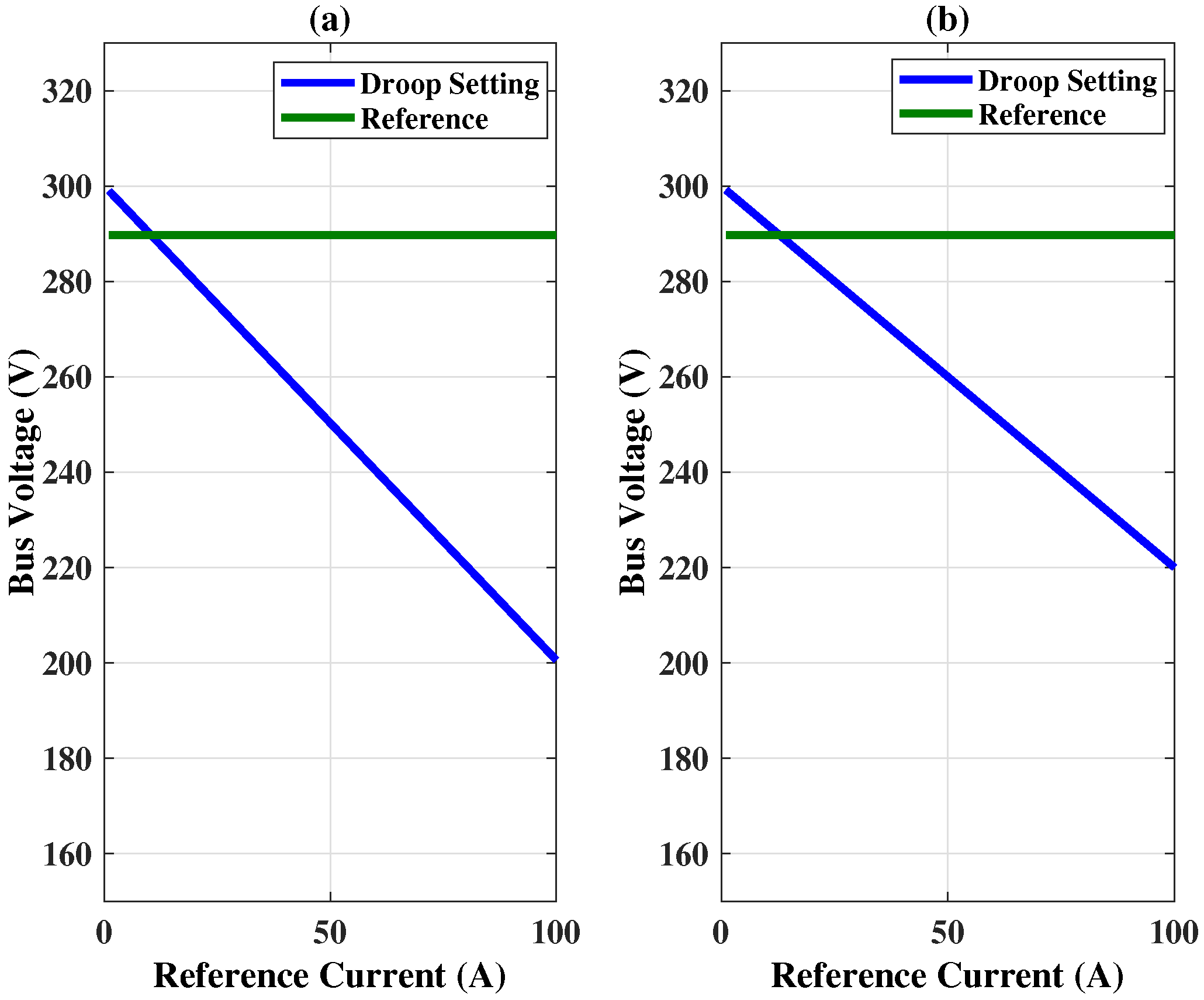
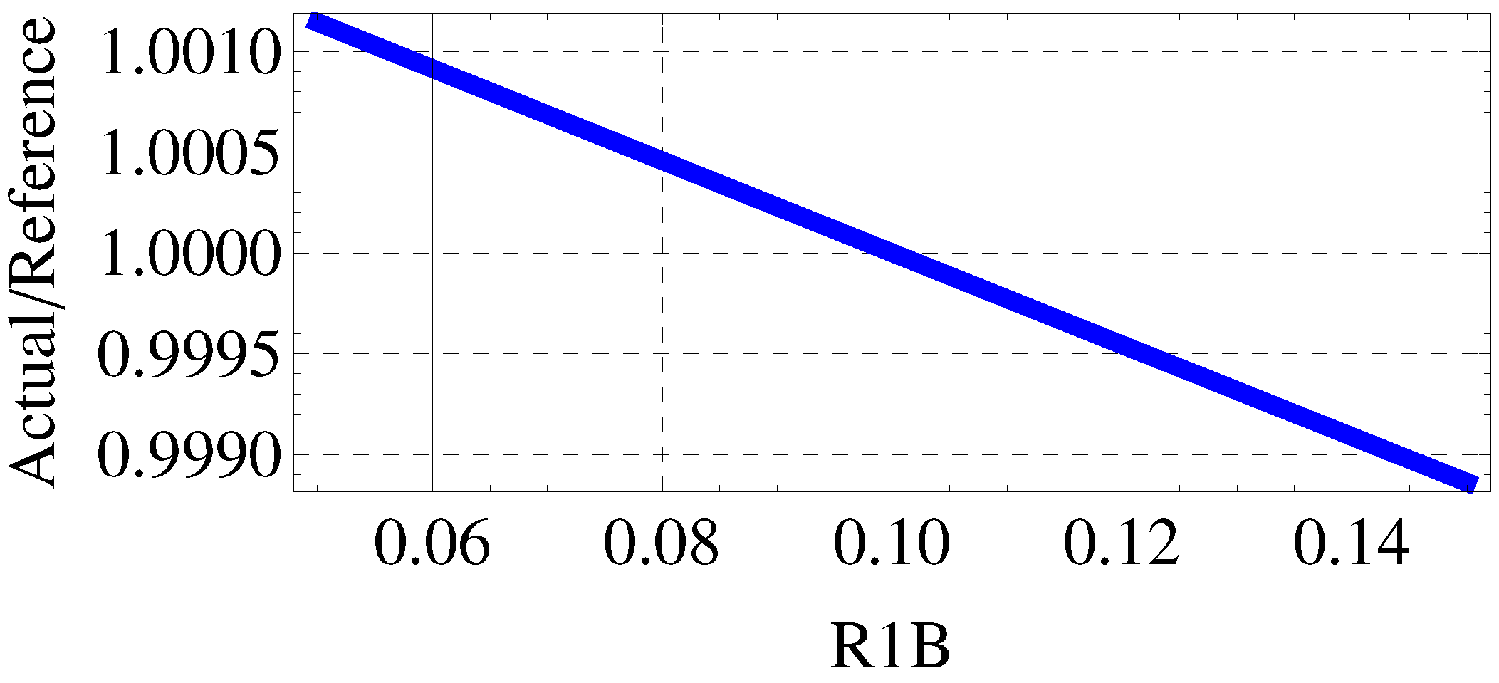
A ratio was calculated to compare the reference current based on the actual resistance value to the reference current based on an assumption of an 0.1 resistance. The result is plotted in Figure 24 over a range of resistances from ±50% from the nominal value. This result shows that even if the line resistance used to calculate the reference current differs within ±50% from the actual line resistance, the impact on the reference current is less than ±0.1%.
5.2. Sensitivity in
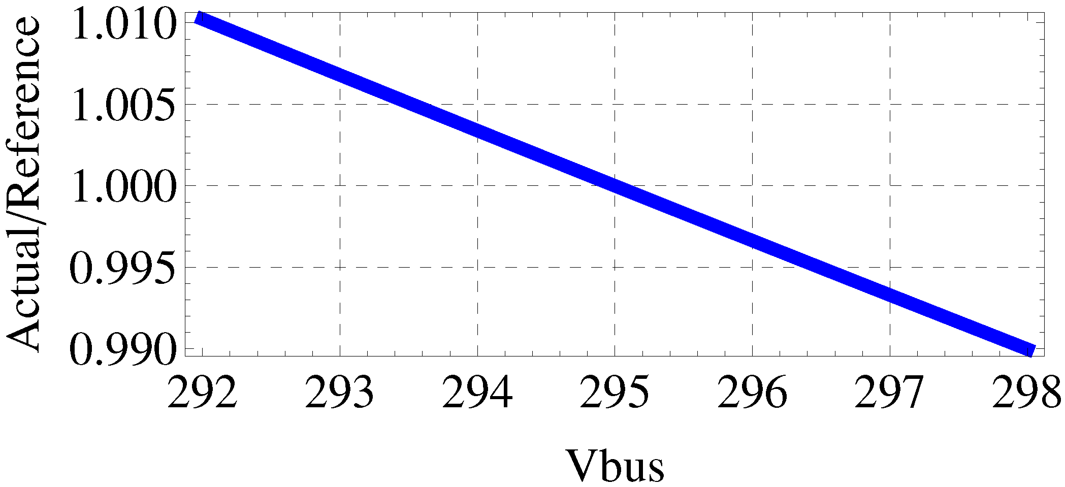
A ratio was calculated to compare the reference current based on the actual bus voltage to the reference current based on an assumption of a bus voltage measurement of 295 V. The result is plotted in Figure 25 over a range of bus voltages from ±1% from the nominal value. This result shows that even if the measured bus voltage used in the controller differs within ±1% from the actual bus voltage, the impact on reference current is also less than ±1%.
The parameter sensitivity analysis presented here demonstrates that small errors in bus voltage measurement and large errors in the line resistance value have a minimal effect on the calculated reference current for optimal multidimensional droop control.
Author Contributions
In this paper, K.J.B completed the literature review, control design, simulation, and hardware-in-the-loop testing, all with supervision and guidance from W.W.W. The paper was written by K.J.B with review and input from W.W.W.
Funding
This work was supported by a National Science Foundation Graduate Research Fellowship (DGE-1051031) and the Army Research Laboratory (W911NF-13-2-0024).
Conflicts of Interest
The authors declare no conflict of interest.
References
- Lasseter, R.; Paigi, P. Microgrid: A conceptual solution. In Proceedings of the 2004 IEEE 35th Annual Power Electronics Specialists Conference, Aachen, Germany, 20–25 June 2004; pp. 4285–4290. [Google Scholar]
- Wang, Y.; Wu, Z.; Li, Z. Research on wind energy distributed generation in microgrid. In Proceedings of the 2010 International Conference on Power System Technology (POWERCON), ZheJiang, China, 24–28 October 2010; pp. 1–6. [Google Scholar]
- Xiang, J.; Wang, Y.; Li, Y.; Wei, W. Stability and steady-state analysis of distributed cooperative droop controlled DC microgrids. IET Control Theory Appl. 2016, 10, 2490–2496. [Google Scholar] [CrossRef] [Green Version]
- Wang, X.; Zhang, H.; Li, C. Distributed finite-time cooperative control of droop-controlled microgrids under switching topology. IET Renew. Power Gener. 2017, 11, 707–714. [Google Scholar] [CrossRef]
- Johnson, B.K.; Lasseter, R.H.; Alvarado, F.L.; Adapa, R. Expandable multiterminal DC systems based on voltage droop. IEEE Trans. Power Deliv. 1993, 6, 1926–1932. [Google Scholar] [CrossRef]
- Luo, F.; Lai, Y.M.; Tse, C.K.; Loo, K.H. A triple-droop control scheme for inverter-based microgrids. In Proceedings of the 38th Annual Conference on IEEE Industrial Electronics Society, Montreal, QC, Canada, 25–28 October 2012; pp. 3368–3375. [Google Scholar]
- Khorsandi, A.; Ashourloo, M.; Mokhtari, H.; Iravani, R. Automatic droop control for a low voltage DC microgrid. IET Gener. Transm. Distrib. 2016, 10, 41–47. [Google Scholar] [CrossRef]
- Nagliero, A.; Mastromauro, R.A.; Ricchiuto, D.; Liserre, M.; Nitti, N. Gain-scheduling-based droop control for universal operation of small wind turbine systems. In Proceedings of the 2011 IEEE International Symposium on Industrial Electronics (ISIE), Gdansk, Poland, 27–30 June 2011; pp. 1459–1464. [Google Scholar]
- Vidyanandan, K.V.; Senroy, N. Primary frequency regulation by deloaded wind turbines using variable droop. IEEE Trans. Power Syst. 2013, 28, 837–846. [Google Scholar] [CrossRef]
- Fazeli, M.; Asher, G.M.; Klumpner, C.; Liangzhong, Y.; Bazargan, M. Novel integration of wind generator-energy storage systems within microgrids. IEEE Trans. Smart Grid 2012, 3, 728–737. [Google Scholar] [CrossRef]
- Chen, J.; Chen, J.; Chen, R.; Zhang, X.; Gong, C. Decoupling control of the non-grid-connected wind power system with the droop strategy based on a DC microgrid. In Proceedings of the 2009 World Non-Grid-Connected Wind Power and Energy Conference, Nanjing, China, 24–26 September 2009; pp. 1–6. [Google Scholar]
- Goya, T.; Omina, E.; Kinjyo, Y.; Senjyu, T.; Yona, A.; Urasaki, N.; Funabashi, T. Frequency control in isolated island by using parallel operated battery systems applying h-infinity control theory based on droop characteristics. IET Renew. Power Gener. 2011, 5, 160–166. [Google Scholar] [CrossRef]
- Wu, L.; Infield, D. Investigation on the interaction between inertial response and droop control from variable speed wind turbines under changing wind conditions. In Proceedings of the 2012 47th International Universities Power Engineering Conference (UPEC), London, UK, 4–7 September 2012; pp. 1–6. [Google Scholar]
- Ghanbari, N.; Mokhtari, H.; Bhattacharya, S. Optimizing operation indices considering different types of distributed generation in microgrid applications. Energies 2018, 11, 894. [Google Scholar] [CrossRef]
- Markvart, T. Microgrids: Power systems for the 21st century? Refocus 2006, 7, 44–48. [Google Scholar] [CrossRef]
- Mizani, S.; Yazdani, A. Design and operation of a remote microgrid. In Proceedings of the 35th Annual Conference of IEEE Industrial Electronics (IECON), Porto, Portugal, 3–5 November 2009; pp. 4299–4304. [Google Scholar]
- Asmus, P. Microgrids, virtual power plants and our distributed energy future. Electr. J. 2010, 23, 72–82. [Google Scholar] [CrossRef]
- Majumder, R. Some aspects of stability in microgrids. IEEE Trans. Power Syst. 2013, 28, 3243–3252. [Google Scholar] [CrossRef]
- Bunker, K.J.; Weaver, W.W. Multidimensional droop control for wind resources in DC microgrids. IET Gener. Transm. Distrib. 2017, 11, 657–664. [Google Scholar] [CrossRef]
- Bunker, K.J.; Weaver, W.W. Optimal geometric control of DC microgrids. In Proceedings of the 2014 IEEE 15th Workshop on Control and Modeling for Power Electronics (COMPEL), Santander, Spain, 22–25 June 2014; pp. 1–6. [Google Scholar]
- Krein, P.T.; Bentsman, J.; Bass, R.M.; Lesieutre, B.L. On the use of averaging for the analysis of power electronic systems. IEEE Trans. Power Electron. 1990, 5, 182–190. [Google Scholar] [CrossRef]
- Ivanovic, Z.R.; Adzic, E.M.; Vekic, M.S.; Grabic, S.U.; Celanovic, N.L.; Katic, V.A. HIL evaluation of power flow control strategies for energy storage connected to smart grid under unbalanced conditions. IEEE Trans. Power Electron. 2012, 27, 4699–4710. [Google Scholar] [CrossRef]
- Yousefpoor, N.; Azidehak, A.; Bhattacharya, S.; Parkhideh, B.; Celanovic, I.; Genic, A. Real-time hardware-in-the-loop simulation of convertible static transmission controller for transmission grid management. In Proceedings of the 2013 IEEE 14th Workshop on Control and Modeling for Power Electronics (COMPEL), Salt Lake, UT, USA, 23–26 June 2013; pp. 1–8. [Google Scholar]
- Texas Instruments. TMS320F28335 Controlcard. 2014. Available online: http://www.ti.com/tool/tmdscncd28335 (accessed on 1 June 2014).
- Krishnan, R.; Bharadwaj, A.S. A review of parameter sensitivity and adaptation in indirect vector controlled induction motor drive systems. IEEE Trans. Power Electron. 1991, 6, 695–703. [Google Scholar] [CrossRef]
Figure 1.
Simple microgrid example with two sources and one load.

Figure 2.
Power curve for a 2-kW wind turbine.

Figure 3.
Step in change in (a) wind speed and (b) power available from the wind, implemented in both simulation and hardware-in-the-loop.
Figure 3.
Step in change in (a) wind speed and (b) power available from the wind, implemented in both simulation and hardware-in-the-loop.

Figure 4.
Simulation results for power supplied by Sources 1 and 2 during a step change in wind speed.
Figure 4.
Simulation results for power supplied by Sources 1 and 2 during a step change in wind speed.

Figure 5.
Typhoon HIL600 with microgrid control board and three TI-F28335 DSP ControlCARDs (two cards were used for this paper). HIL, Hardware-In-the-Loop.
Figure 5.
Typhoon HIL600 with microgrid control board and three TI-F28335 DSP ControlCARDs (two cards were used for this paper). HIL, Hardware-In-the-Loop.

Figure 6.
Hardware-in-the-loop schematic for the small microgrid example.

Figure 7.
HIL controller for Source 1: optimal multidimensional droop.

Figure 8.
HIL controller for Source 2: traditional droop.

Figure 9.
Hardware-in-the-loop results with optimal multidimensional droop control during a step change in wind speed: Ch1 bus voltage; Ch2 Source 1 current; Ch3 Source 2 current.
Figure 9.
Hardware-in-the-loop results with optimal multidimensional droop control during a step change in wind speed: Ch1 bus voltage; Ch2 Source 1 current; Ch3 Source 2 current.

Figure 10.
Simulation and hardware-in-the-loop results for bus voltage during a step change in wind speed.
Figure 10.
Simulation and hardware-in-the-loop results for bus voltage during a step change in wind speed.

Figure 11.
Simulation and hardware-in-the-loop results for Source 1 current during a step change in wind speed.
Figure 11.
Simulation and hardware-in-the-loop results for Source 1 current during a step change in wind speed.

Figure 12.
Simulation and hardware-in-the-loop results for Source 2 current during a step change in wind speed.
Figure 12.
Simulation and hardware-in-the-loop results for Source 2 current during a step change in wind speed.

Figure 13.
Example microgrid for the demonstration of droop control methods.

Figure 14.
(a) Load and (b) wind speed profiles for the simulated 24-h period.

Figure 15.
Power curve for the 12-kW wind turbine.

Figure 16.
Linear droop control relationships for (a) wind source and (b) conventional source for first simulation.
Figure 16.
Linear droop control relationships for (a) wind source and (b) conventional source for first simulation.

Figure 17.
Simulation results using traditional droop control: (a) power supplied by each source; (b) power consumed by each load; and (c) power supplied by the battery.
Figure 17.
Simulation results using traditional droop control: (a) power supplied by each source; (b) power consumed by each load; and (c) power supplied by the battery.

Figure 18.
Multidimensional droop control relationship for the second simulation.

Figure 19.
Simulation results using multidimensional droop control: (a) power supplied by each source; (b) power consumed by each load; and (c) power supplied by the battery.
Figure 19.
Simulation results using multidimensional droop control: (a) power supplied by each source; (b) power consumed by each load; and (c) power supplied by the battery.

Figure 20.
Optimal multidimensional droop control relationship for the third simulation.

Figure 21.
Simulation results using optimal multidimensional droop control: (a) power supplied by each source; (b) power consumed by each load; and (c) power supplied by the battery.
Figure 21.
Simulation results using optimal multidimensional droop control: (a) power supplied by each source; (b) power consumed by each load; and (c) power supplied by the battery.

Figure 22.
Power supplied from (a) wind source and (b) conventional source using 2D, 3D and optimal 3D droop. Power available from the wind is also shown.
Figure 22.
Power supplied from (a) wind source and (b) conventional source using 2D, 3D and optimal 3D droop. Power available from the wind is also shown.

Figure 23.
Microgrid bus voltage with (a) optimal multidimensional droop control, (b) multidimensional droop control and (c) traditional droop control.
Figure 23.
Microgrid bus voltage with (a) optimal multidimensional droop control, (b) multidimensional droop control and (c) traditional droop control.

Figure 24.
Ratio of the actual to ideal reference current with respect to line resistance.

Figure 25.
Ratio of actual to ideal reference current with respect to measured bus voltage.


Table 1.
Microgrid parameter values.
| Component | Value | Unit |
|---|---|---|
| 0.1 | ||
| 1 | mH | |
| 0.2 | ||
| 2 | mH | |
| 1 | mF | |
| 100 | V | |
| 1 | ||
| 1 | ||
| 10 |
Table 2.
HIL analog output configuration. AO, Analog Output.
| AO Channel | Model Parameter | Scaling |
|---|---|---|
| 1 | 100 V per 1 | |
| 2 | 10 A per 1 | |
| 3 | 10 A per 1 | |
| 4 | 100 V per 1 | |
| 5 | 100 V per 1 |
Table 3.
Source 1 and Source 2 parameter values.
| Source 1 | Source 2 | ||||
|---|---|---|---|---|---|
| Component | Value | Unit | Component | Value | Unit |
| 400 | V | 380 | V | ||
| 0.2 | 0.2 | ||||
| 0.2 | mF | 0.2 | mF | ||
| 1.5 | mH | 1.5 | mH | ||
| 0.08 | F | 0.08 | F | ||
| 5 | mH | 5 | mH | ||
| 0.1 | 0.23 | ||||
| 1.2 | mH | 0.8 | mH | ||
| 300 | V | 300 | V | ||
| 0.9 | 0.8 | ||||
| 1 | 1 | ||||
| 10 | 10 | ||||
| 1 | 1 | ||||
| 10 | 10 |
Table 4.
Comparison of unused energy from the wind for three droop control methods, in a full microgrid example.
Table 4.
Comparison of unused energy from the wind for three droop control methods, in a full microgrid example.
| Droop Control Strategy | Reference Current Equation | Unused Energy (W-h) |
|---|---|---|
| Linear | 149,770 | |
| Planar | 39,792 | |
| Optimal Surface | 2651 |
© 2018 by the authors. Licensee MDPI, Basel, Switzerland. This article is an open access article distributed under the terms and conditions of the Creative Commons Attribution (CC BY) license (http://creativecommons.org/licenses/by/4.0/).
Share and Cite
MDPI and ACS Style
Bunker, K.J.; Weaver, W.W. Optimal Multidimensional Droop Control for Wind Resources in DC Microgrids. Energies 2018, 11, 1818. https://doi.org/10.3390/en11071818
AMA Style
Bunker KJ, Weaver WW. Optimal Multidimensional Droop Control for Wind Resources in DC Microgrids. Energies. 2018; 11(7):1818. https://doi.org/10.3390/en11071818
Chicago/Turabian StyleBunker, Kaitlyn J., and Wayne W. Weaver. 2018. "Optimal Multidimensional Droop Control for Wind Resources in DC Microgrids" Energies 11, no. 7: 1818. https://doi.org/10.3390/en11071818
Note that from the first issue of 2016, this journal uses article numbers instead of page numbers. See further details here.