Quantile Regression Post-Processing of Weather Forecast for Short-Term Solar Power Probabilistic Forecasting


CRS4, Center for Advanced Studies, Research and Development in Sardinia, loc. Piscina Manna ed. 1, 09010 Pula (CA), Italy
*
Author to whom correspondence should be addressed.
Energies 2018, 11(7), 1763; https://doi.org/10.3390/en11071763
Submission received: 11 May 2018
/
Revised: 25 June 2018
/
Accepted: 28 June 2018
/
Published: 4 July 2018
(This article belongs to the Special Issue Solar and Wind Energy Forecasting)
Abstract
:The inclusion of photo-voltaic generation in the distribution grid poses technical difficulties related to the variability of the solar source and determines the need for Probabilistic Forecasting procedures (PF). This work describes a new approach for PF based on quantile regression using the Gradient-Boosted Regression Trees (GBRT) method fed by numerical weather forecasts of the European Centre for Medium Range Weather Forecast (ECMWF) Integrated Forecasting System (IFS) and Ensemble Prediction System (EPS). The proposed methodology is compared with the forecasts obtained with Quantile Regression using only IFS forecasts (QR), with the uncalibrated EPS forecasts and with the EPS forecasts calibrated with a Variance Deficit (VD) procedure. The proposed methodology produces forecasts with a temporal resolution equal to or better than the meteorological forecast (1 h for the IFS and 3 h for EPS) and, in the case examined, is able to provide higher performances than those obtained with the other methods over a forecast horizon of up to 72 h.
1. Introduction
The inclusion of renewable generation in distribution grids poses technological challenges that need to be addressed to achieve technically and economically sustainable integration. One of the difficulties is linked to the variability of the solar source, which does not guarantee a flexible production, but depends on the weather conditions and may be subject to strong variations in the short term in relation to cloud cover. This is one of the reasons why the current regulations governing the electricity market in various regions favor the definition of a production profile one day in advance [1,2,3].
Apart from the demand-side management, the energy storage and the generation and load forecasts are the most promising strategies to reduce the negative impact of the variability of renewable energy production for a small grid, particularly for use on an island [4]. These strategies are one of the topics studied in the European H2020 NETfficient to which this work is related. The project aims to propose an effective innovation in the use and distribution of electric power through the development of several energy storage technologies and an energy management system, enabling the implementation of a smart grid on the German island of Borkum in the North Sea.
The recent Global Energy Forecasting Competition (GEFCOM 2014) included a line of analysis for predicting the power generated by PV systems. In the presentation editorial [5], Hong et al. indicated a low level of maturity for the prediction of PV power, both deterministic and probabilistic, when compared with other areas of energy forecasting, such as wind power generation or grid load forecasting. For the authors, this was linked to the low penetration of PV production in the electricity markets.
The forecast of Photo-Voltaic (PV) production is traditionally deterministic; however, this approach does not provide information that could be very useful for utility managers such as the forecast error margins and the confidence one can have in the forecast [6]. Instead, a probabilistic forecast, besides indicating the most probable value of the power generated by the system, can estimate a range of plausible values and the probabilities associated with them, and it is useful in all those activities that require risk and uncertainty management, such as for example balancing the loads of a network or buying and selling energy in the market. The literature on the probabilistic forecasting of PV production is less rich than that on wind generation or grid load forecasting. A very recent and accurate review can be found at [7].
One of the first works that addressed the prediction of PV energy production with a non- parametric probabilistic approach was written by Bacher et al. [8]. In their study, the authors used power measurements from 21 PV systems to predict generation up to 36 h in advance with an autoregressive analysis of the historical series and then enriching the method with the exogenous input of meteorological variables obtained from Numerical Weather Predictions (NWP). In the same year, there was the work of Lorenz et al. [9], whose objective was to obtain a probabilistic forecast of the production of 11 plants in southern Germany with a time horizon of up to three days, an hourly resolution and using the weather forecasts of the Ensemble Prediction System (EPS) of the European Centre for Medium Range Weather Forecast (ECMWF). Later, Monteiro et al. in [10] proposed a model called HISIMIbased on historical similarity. Historical values of power generation are grouped into intervals, and the result of the prediction is the probability that the power produced will fall into each of the selected intervals. Bracale et al. in [11] obtained a probability distribution for predicting the power generated from a Bayesian autoregressive model that takes into account the dependence on solar radiation and some weather variables, such as cloud cover and humidity. Most recently, Almeida et al. [12] studied the accuracy of the non-parametric probability forecasts using the quantile regression forest methodology for five PV plants in northern Spain. The authors used different variables of the meteorological model and showed the importance of the radiation data and the scarce utility of the increase in the number of variables used in the modeling. Alessandrini et al. in [13] proposed a methodology called Analog Ensemble (AnEn) and compared it to the benchmark represented by the Persistence Ensemble (PeEn) and the quantile regression for three PV plants in Italy. AnEn has shown superior performance compared to other methods and has produced a more reliable predictive density. The method uses limited-area weather forecasts for the three plants with an hourly resolution and a 72-h horizon. Huang and Perry forecasted the hourly electricity generation of three PV plants with ECMWF data [14]. A separate model was created for each hour when the solar radiation was non-zero, using a gradient-boosted regression trees technique. The probabilistic forecast intervals were instead estimated using a k-nearest neighbors regression procedure. Pierro et al. [15] created a multi-model forecast ensemble with forecasts of two different weather models, obtaining performances superior to the best among the members of the forecast ensemble. The main reason for this was the ability of the ensemble averaging to reduce the noise of individual predictors. In general, it was also found that the models generated more accurate forecasts using ECMWF data than the Weather Research and Forecasting regional model (WRF). In [16], Sperati et al. used the EPS to produce a probabilistic forecast with a horizon of up to 72 h and a resolution of 3 h. The members of the ensemble are processed by a neural network to obtain the forecasts of photo-voltaic production, and these data are then elaborated statistically to correct the under-dispersive characteristics. For this reason, two techniques called Variance Deficit (VD) and Ensemble Model Output Statistics (EMOS) were used, and their performances were compared with the PeEn benchmark previously used by the authors themselves. Rana and Koprinska in [17] presented a methodology for the prediction of a range of variability of energy production, obtained through an ensemble of neural networks, but not using the forecast of meteorological models as an input feature. The results for short-term forecasting in comparison with benchmark methodologies are promising. In [18], Mohammed and Aung proposed to realize the prediction of the production of three solar farms 24 h in advance, using the deterministic meteorological forecast of the ECMWF model, with a total of seven different regression methodologies and combining them with three different ensembles of methods. The results showed that the individual methods all offer superior performance to traditional time series analysis techniques and that their evaluation as an ensemble can guarantee even greater accuracy.
Compared to the bibliography, in this article, we propose an innovative methodology to obtain probabilistic forecasts of the energy production of a PV system, with hourly resolution and a forecast horizon of up to 72 h, in which ECMWF ensembles and deterministic forecasts are used together as features for a quantile regression. The single deterministic forecast, necessary to obtain the ensemble members, is obtained by means of a regression model based on the Gradient-Boosted Regression Trees (GBRT) technique and using as input some of the results of the operational forecasts of the IFS ECMWF model [19]. The technique adopted allows us to obtain forecasts with an equal or higher temporal resolution than that of the meteorological output, through the use of a production index. This is very important in order to exploit the results of the EPS system [19], which have a time resolution of 3 h, lower than that of the IFS deterministic model (1 h).
As a benchmark, to assess the effectiveness of the proposed new methodology, probability forecasting is obtained through five different models:
- The Quantile Regression (QR) uses a GBRT methodology and generates an ensemble of forecasts based on the IFS forecasts of the ECMWF model and the plant power output measured previously under similar conditions.
- The Ensemble Prediction System (EPS) uses the results of the EPS weather forecast ensemble of the ECMWF model, processed through the regression model used in deterministic prediction, and no calibration or ensemble post-processing technique.
- The Variance Deficit (VD) applies the variance deficit calibration technique to the results of the EPS model.
- The Quantile Ensemble (QE) still uses the EPS forecasting ensemble and the plant model, but applies a post-processing procedure based on quantile regression with the GBRT methodology to the predictions obtained.
- The Quantile Ensemble Plus (QE+) is similar to the previous one, but uses both the IFS and EPS forecasts of the ECMWF model as features in quantile regression, in order to make the most of the information that can be extracted from both weather models.
The points that the article will highlight as elements that contribute to obtaining a quality forecast, and that for the sake of clarity we list as items, are the following:
- the use of the power index to efficiently forecast solar power generation even with temporally-coarse weather forecasts;
- the effectiveness of the gradient-boosted quantile regression trees for the post-processing of the ensemble of predictions from the EPS;
- the relative importance of the EPS and IFS forecasts of the ECMWF depending on the forecast horizon considered;
- the combined use of the IFS and EPS forecast of ECMWF for an accurate probabilistic and deterministic PV power forecast.
The remainder of the paper is organized as follows. In Section 2, the modeling procedure is described. The metrics adopted to measure the accuracy of the deterministic and probabilistic forecast are presented in Section 3. The results are presented in Section 4 and discussed in Section 5, finally, in Section 6, the conclusions and future directions are drawn.
2. Methods
The power that can be obtained from a PV system is almost entirely related to the solar radiation incident on the panels. The solar radiation that reaches the upper part of the Earth’s atmosphere oscillates around the solar constant [20], modulated in the path to the Earth’s surface due to reflections, absorption and re-emissions from the various layers of the atmosphere. The radiation that finally reaches the Earth’s surface is divided into two distinct components, namely direct and diffuse irradiation. The first component, known as Direct Normal Irradiation (DNI), is associated with energy coming directly from the Sun following the direction of its rays; the second component reaches the surface indirectly, derives from the portion of radiation scattered by the atmosphere and appears as diffused from the sky. The ground projection of the scattered radiation is indicated as Diffuse Horizontal Irradiation (DHI). The sum of the direct and diffuse radiation projected to the ground is the Global Horizontal Irradiation (GHI) [21].
where is the solar zenith angle.
Whenever possible for medium-sized power plants, the solar panels are oriented to maximize the energy generated during the year. The radiation that reaches a non-horizontal surface is given by the sum of the projections of the direct and diffuse components of solar radiation, the net of any obstacles and shading. The irradiation on the Plane Of Array (POA) is calculated as [22]:
where denotes the beam component, denotes the ground-reflected component and denotes the sky-diffuse component. The beam component of the solar irradiation corresponds to the projection of the DNI on the surface [22]:
where AOI denotes the Angle Of Incidence between the Sun’s rays and the surface. The sky-diffuse component is calculated from the DHI and the orientation of the panel. Several models are available, the simplest being the isotropic model [22]:
where is the tilt angle of the panel plane.
It may be useful to determine the radiation conditions (DNI, DHI and GHI) in cloud-free conditions, by using the so-called clear sky models [21]. These models give a theoretical limit to the values of solar radiation for a given place with time variation. Clear sky radiation models are developed using Radiative Transfer Models (RTM) and require knowledge of local weather variables such as ozone and water vapor content in the atmosphere, Linke turbidity and the relative position of the Sun [23]. A recent comparison of these parametric models [24] revealed that even simple models based on standard atmospheric composition, such as ESRA models [25] or Ineichen [23], can give satisfactory results if accurate meteorological information is not available.
The actual radiation conditions can be compared with the ideal clear sky conditions by using the k index, commonly used in the literature and defined as:
A clear sky performance index is also introduced, , following [8] and as already done in [26], defined as the ratio between the power actually developed by a PV system in a given moment and that which the same system would ideally have produced in clear sky conditions:
The clear sky power is estimated as follows:
where denotes the peak power of the plant and denotes a reference irradiation. is calculated with Equations (2)–(4), in which the values of GHI and DHI are obtained from the clear sky model for the location of the plant.
2.1. Gradient-Boosted Regression Trees
A data-driven approach was used to predict the power generated by the PV system, fitting a regression model based on the gradient-boosted regression trees technique [27] as implemented in [28]. GBRT is a machine learning technique for regression and classification problems. This is a particularly effective regression technique for datasets with a limited number of samples, unlike recurrent neural networks and has proven effective in predicting PV production; see, for example, [14] and [18].
Similar to other boosting algorithms, GBRT builds a model as a weighted sum of functions:
where are the basis functions, which are usually called weak learners and in this case are decision trees of fixed size. M is the number of weak learners used. The model is built gradually in a forward stage-wise fashion:
where n is the number of samples. At each stage, the decision tree is chosen to minimize the loss L given the current model and its fit . The so-called pseudo-residuals are computed:
and is fitted using as the target variable.
The weights are obtained by solving a minimization problem:
The loss for the deterministic forecast is the square error:
The following expression is used for quantile regression, where is the required quantile (a value between 0 and 1):
2.2. Deterministic Forecasting
In real cases, it is often necessary to make predictive models starting from a set of data of limited duration, especially in the initial phase of management of a power plant. In our case, we had only one year of data and were therefore interested in developing a solution, supported by a limited number of samples, capable of providing both a deterministic forecast and a measure of its uncertainty. In such cases, the use of a large number of features inevitably exposes a regression procedure to the problem of over-fitting, so it was necessary to select the minimum number of features that could be effective in the creation of the model. The result of a systematic research, previous experiences on the same dataset [26] and the analysis of physical models for PV systems led us to the adoption of the procedure described below.
The model uses astronomical data (the relative position of the Sun expressed as zenith and azimuth angles) and the output of a weather forecast model, in particular the estimation of GHI, the precipitation and the temperature at 2 m above ground level. GHI is introduced through the k index defined in the previous Equation (5). The regression is not carried out on the generated power, but on the index defined by Equation (6). The choice to use the ratios with the reference of the clear sky model allows us to treat more easily the averaged quantities, which constitute the output of the meteorological model, and to obtain forecasts with a temporal resolution that is not affected by that of the meteorological model. The feature used to describe the precipitation forecast is Boolean and states only the possibility of rain.
Therefore, the deterministic model can be used to estimate the performance index :
where is the possibility of rain ({0,1}), the temperature 2 m above the ground and and are the zenith and azimuth angles of the Sun. The estimate of the power generated by the system is then obtained as:
The model is trained using the ECMWF IFS forecast for the point closest to the installation position with a horizon of up to 24 h, generating a complete time series with hourly frequency. The power index used in the training is calculated from the ratio between the hourly averages of the measured and clear sky power. The deterministic forecast with hourly resolution and forecast horizon up to 72 h is then obtained by applying the model to the output of the IFS.
2.3. Quantile Regression
The method uses the same regression technique as the one used for the deterministic forecast (GBRT), but with a quantile loss function. Several models of quantile regression are therefore produced, one for each quantile examined. To allow a direct comparison with the methodologies based on the EPS, an ensemble of 51 models is realized corresponding to values of quantiles uniformly distributed in the open range . As in the case of the deterministic prediction, the model allows us to obtain a forecast of the power index , for each of the 51 quantiles; the actual power is then obtained from the product of the power index for the clear sky power , as for Equation (16). This model is referred to as QR.
2.4. Ensemble Probabilistic Forecasting
The deterministic model obtained with the GBRT regressors trained on the IFS data and measured power is applied to obtain a probabilistic prediction of the power produced through the processing of the output of the EPS. EPS is based on singular vector perturbation of the initial conditions of the atmospheric model and on stochastic perturbations of some parameters of the physical parameterization of the meteorological model. EPS then simulates the evolution of 50 different equiprobable scenarios for each atmospheric variable of interest plus that for an undisturbed forecast (i.e., the Control Forecast: CF). The 50 members of EPS and the CF are then used to obtain a set of 51 forecasts of the generated power. The meteorological data have a resolution of 3 h, and the GHI, precipitation and soil temperature data are representative of the average value of that quantity in the 3-h time interval. The GHI is inserted in the model as a ratio of k with respect to the average GHI value evaluated in clear sky conditions. The values of the index k, the average precipitation and the average temperature are assumed constant in the range of 3 h and re-sampled to obtain a forecast with hourly resolution. These new time series can be inserted into the model together with the astronomical data, always with hourly resolution, to obtain a forecast of the performance index and, finally, with Equation (16), a set of 51 forecasts for the power produced. The model is referred to as EPS in the following paragraphs.
2.5. VD Calibration
The ensemble obtained with the EPS method must be subject to a calibration procedure with the aim of making the average spread of the ensemble as similar as possible to the standard deviation of the observations. A calibration procedure known as variance deficit can be applied for this purpose. A first transformation allows us to change the range of variation from to :
Each of the 51 power forecasts is then transformed by a Generalized Logit (GL) transformation [29].
where the shape parameter influences the evolution of variance and skewness of these distributions as a function of their mean. The values of the forecast ensemble obtained with the EPS model are altered linearly with a constant coefficient of proportionality for each moment and keeping the average unchanged:
where is the ensemble mean. The coefficient is calculated as:
where is the transformation using Equations (17) and (18) of the measured power and is the standard deviation of the ensemble at the time .
2.6. Quantile Ensemble
A procedure is proposed for the construction of an ensemble of the powers generated, on the basis of the results of the EPS model and the deterministic regression model. The procedure is based on the construction of a quantile regression using gradient-boosted regression trees on the results of the application of the deterministic regression model to the forecast ensemble of the EPS model, similarly to what has been proposed in the meteorological context by Taillardat [30].
A first version of the procedure, indicated as QE in the following, may be divided into the following steps:
- The deterministic model is applied to the ECMWF EPS forecasts, generating an ensemble of 51 power forecasts for the plant
- For each time step, 9 quantiles [0.1, 0.2, …, 0.9] are used to describe the distribution of the ensemble and constitute a set of new features.
- Fifty one GBRT quantile regressors are trained, choosing the quantile of the target function, in the quantile range [1/52, 2/52, …, 51/52], using as input features the 9 quantiles with which the distribution of power forecasts for the training period is represented and, as the training variable, the power actually measured.
The result of the model in turn constitutes an ensemble of forecasts, with 51 members representing the quantiles of the power distribution forecast, the number of members being chosen equal to that of the EPS and VD models to ease the comparison. In order to formulate the predictions, the forecast ensemble required information on the representative model of the generating plant, the results of the EPS model and historical data on the power distribution for given weather conditions. The use of quantiles to represent the distribution of the members of the ensemble as features of the regressor implies that this can be considered more of a post-processing than a calibration methodology, as it loses some of the information related to the spatial-temporal structure of the members. The model and its results are referred to as QE below.
2.7. Quantile Ensemble Plus
The procedure described previously is refined, using the deterministic forecast obtained from the results of the high resolution IFS model as an input feature, in addition to the 9 quantiles descriptive of the EPS forecast, for a total of 10 features. The quantile regression follows the same procedure as described above and leads to the creation of an ensemble of forecasts of 51 members. This ensemble includes information about the distribution of the powers measured in the training set for certain weather conditions, the descriptive model of the system, EPS forecasts and high-resolution IFS forecasts. The model is referred to as QE+ below.
2.8. Implementation
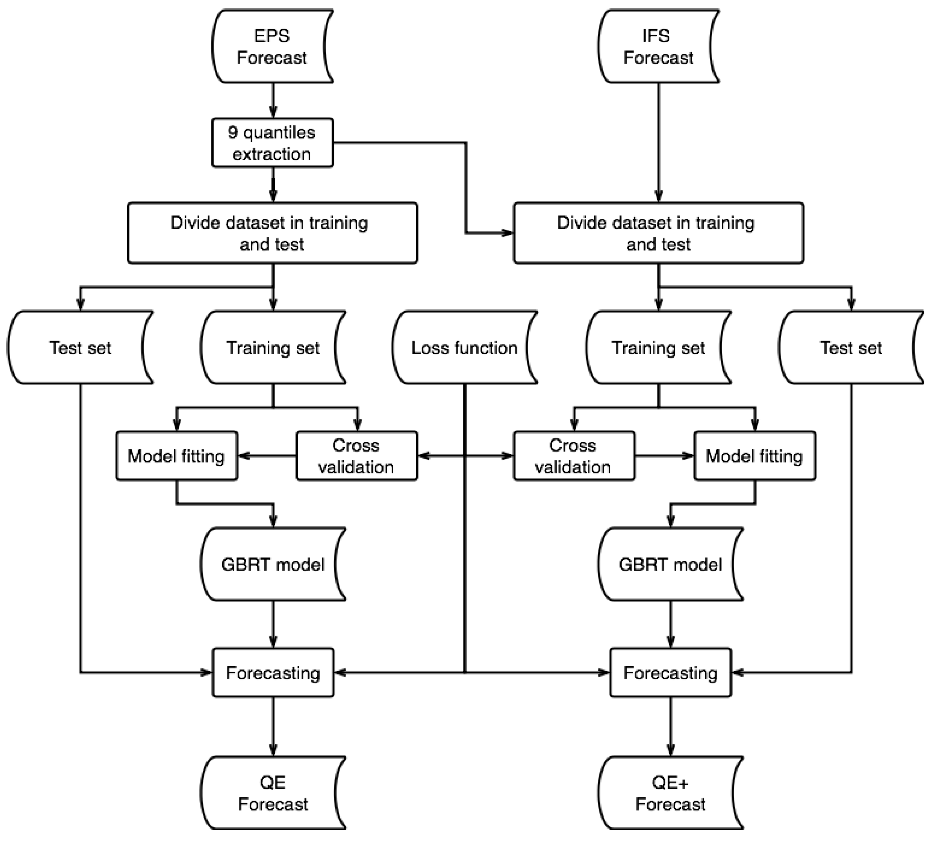
The procedures described were implemented using only public domain tools. The code is written entirely in Python, using the pandas libraries [31], pvlib [32] for the clear sky model and for Sun positioning and scikit-learn [28] for machine learning tools. All libraries have been used in the latest revision available at the time of writing. The procedure requires a standard desktop computer for its execution with overall calculation times lower than an hour in the learning phase for model selection and fitting and almost instantaneous in that of prediction. In order to improve the comprehension of the QE and QE+ procedure, a detailed flowchart describing the algorithm is shown in Figure 1.
3. Forecast Verification
Some well-known accuracy metrics will be used in the following to assess the quality of the deterministic forecast. Specifically, the Mean Error (ME), the Mean Absolute Error (MAE) and the Root Mean Square Error (RMSE). The same indicators will also be calculated relative to the PV plant peak power and are called normalized Mean Error (nME), normalized Mean Absolute Error (nMAE) and normalized Root Mean Square Error (nRMSE):
where is the actual power, is the estimated power at time and N is the number of observations. Finally, the quality of correlation between two variables will be measured by the coefficient of determination (), where is the mean value of the actual power:
Skill scores are widely used in assessing the performance of weather forecasting methods. They are defined as a measure of the relative improvement of a forecasting method over a reference. A commonly-used reference is the persistence forecast, the simplest method to predict the production of a PV plant that predicts that the production on a given day will be the same as on the previous day for a lead time of 24 h. Using the RMSE as a measure of accuracy, the Skill Score (SS) is defined as [33]:
where and are the root mean square error of the forecast method and of the persistence, respectively. The higher the skill score, the better.
For the probabilistic forecast, apart from the deterministic indicators that will be calculated relative to the ensemble median, the quality of some probabilistic forecasting aspects will be evaluated by using a set of specific indicators, a detailed discussion of which can be found in [34].
A measure of how the ensemble spread consistently represents the uncertainty of the observations can be obtained through the rank histogram. This chart shows the frequency of observations for each forecast probability class. If the probability distribution of the forecast reproduces on average the probability distribution of the observations, then this diagram should be flat, indicating that each member of the ensemble is equally probable. The ensemble spread can be modified adaptively using an appropriate calibration procedure that makes the ensemble and observation variability, with respect to the ensemble mean, statistically indistinguishable. This procedure, called ensemble calibration, improves the rank histogram features without substantially altering the other indicators (see Section 2.5).
Another measure is given by the Receiver Operating Characteristic curve, i.e., ROC curve. It is a graphical plot that illustrates the diagnostic ability of a binary classifier system as its discrimination threshold is varied. The ROC curve is obtained by plotting the true positive rate vs. the false positive rate, using increasing probability thresholds. In addition to the diagram, the measure of the Area Under the ROC Curve (AUC) will be utilized as a global score, which in the ideal case should be 1.
Another measure of the performance of a binary classifier is the Brier Score (BS):
where P and are the probabilities that the observed and predicted power would exceed a fixed threshold. Clearly, P can only assume values of 1 or 0, as well as in the case of deterministic forecasts. Instead, for the ensemble forecast, will assume a value expressed by a rational number between 0 and 1. The number of probability classes will be in that case fixed by the number of members of the ensemble.
The Brier score can be decomposed into 3 additive components: uncertainty, reliability and resolution [35].
where K is the number of discrete values of the probability , the observed climatological base rate for the event to occur, the number of forecasts with the same probability value and the observed frequency.
In the BS decomposition, the uncertainty term measures the variability in the observations (i.e., the difficulty of the forecast situations). The reliability term measures how well the conditional relative frequency of events matches the forecast. It is a measure of the calibration: if the reliability is 0, the forecast is perfectly calibrated. The resolution term measures how well the forecasts distinguish situations with different frequencies of occurrence; the higher this term is, the better.
An indicator, as the BS, based on a single number once a threshold has been set, provides an immediate, but incomplete indication of the forecast quality. The Continuous Ranked Probability Score (CRPS) may be calculated for continuous quantities. CRPS is the equivalent of the BS, integrated over all possible thresholds, and is given by:
where is the Cumulative Distribution Function (CDF) of the probabilistic forecast for the i-th value, while is the CDF of the observations. Note that the CPRS coincides with the MAE for a deterministic forecast [36]. Small values of CRPS indicate good performances.
4. Results
The forecast procedure was tested on a medium-sized PV plant located on the German island of Borkum, oriented south, with a tilt angle of 38 deg and an approximate peak power of 1.3 MW. The data of the power produced by the plant were available for the year 2014 as a complete time series with a time interval of 15 min; see Table 1.
The weather forecasts of radiation, total precipitation and temperature 2 m above ground are provided by the IFS and EPS ECMWF operational models [19]. For the year examined, the IFS model was the TL1279L137 (horizontal resolution equivalent to an average of 9 km with 137 vertical levels). The EPS model is based on an ensemble of 50 forecast starting from perturbed initial conditions, in addition to the CF obtained from the unperturbed initial condition. The model used for EPS is the T639 (equivalent to an average horizontal resolution of 18 km).
The data were collected from the ECMWF MARS archive for 00 UTC analysis and forecast time up to 72 h with a prediction interval of 1 h for the IFS forecast and 3 h for the EPS.
The deterministic model of the plant is obtained through the gradient-boosted regression trees technique, using as features the GHI’s clear sky index k, the precipitation (expressed as binary variable), the air temperature at 2 m above ground and the angles of the zenith and azimuth of the apparent position of the Sun. The model is trained on the performance index , that is the ratio between the measured power and the power that the system would theoretically have developed in clear sky conditions. The forecast of the output power is obtained from the product of the power index forecast for the clear sky power.
Starting from the measured power data, a time series is obtained for the average power with an hourly rate, therefore equal to that of the weather forecasts of the IFS model. The deterministic model is trained using the IFS’s forecast with a horizon of up to 24 h assuming that it is the closest to real conditions. In the forecasting phase, the model is then applied for forecasts up to 72 h as three separate forecasts for each of the days of the forecasting horizon.
The input data are divided into training and test sets, considering the first 10 days of each month for the latter, and using the remaining part of the year for model training. The choice of the model parameters is realized through a cross-validation procedure with a grid search algorithm. The parameters of the model on which the search is conducted are shown in Table 2, which also shows the values that were optimal for the regressors used for the deterministic model and for the QE and QE+ procedures. Three-fold cross-validation is used, in which the training set is randomly partitioned into three equally-sized subsets. A single subset is retained as the validation data for testing the model, and the remaining data are used for the training. The process is repeated for each of the three subsets, and the results are averaged to produce a single estimation. The relative feature importances for the deterministic model are listed in Table 3.
The same regression technique, the same breakdown in training and test sets and the choice of parameters via cross-validation and grid search are also used for the 51 models of the quantile regression and for the ensemble post-processing in the QE and QE+ models.
Table 4 reports the errors for the forecast of the deterministic model for the three forecast days. The errors are relative only to the instants in which the zenith angle of the Sun is less than and there can therefore be power generation. The bias remains minimal for the three days, while the MAE and RMSE values inevitably increase with the forecast horizon time, due to the increased uncertainty of the IFS forecast.
The results obtained using the five probabilistic forecast methods (QR, EPS, VD, QE, QE+), described in detail in Section 2.2, Section 2.3, Section 2.4, Section 2.5, Section 2.6 and Section 2.7, are now compared. Each of the procedures described generate an ensemble of 51 predictions, in order to facilitate the comparison.
An initial evaluation of the quality of the models studied involves verifying the statistical consistency of the ensembles produced. A first desirable feature is that the members of the ensemble are indistinguishable from the observations.
One of the methods used for this assessment is represented by the rank histogram. Figure 2 shows the rank histograms related to the methods considered for forecast in the 24–48-h range, and the horizontal line identifies the optimum of a perfectly-calibrated ensemble. It is noted that the EPS method is far from the optimal condition and shows a markedly under-dispersive behavior, i.e., it cannot adequately describe the variability of the measurements. The calibration that can be performed with the variance deficit method does not appear fully satisfactory; the shape parameter is chosen so as to minimize the CRPS value on the training set, resulting in in our case, but the rank histogram still appears under-dispersive. QR and QE methods produce, instead, much more satisfactory results.
The different methods are then compared on the basis of their ability to predict the probability of exceeding a given threshold. For this purpose, the threshold must necessarily be variable during the day and the time of year, since for example, establishing that half of the rated power of the plant is exceeded has a completely different meaning in the summer months compared to the winter months or also during the day. A natural choice is therefore represented by the threshold defined as a fraction of the clear sky power, variable during the day and the time of the year, and compare the forecasts of exceeding this threshold as provided by the models, with the events that actually occurred.
A first measure of the accuracy of these predictions is the Brier score. The Table 5 reports the values for the methods examined for a threshold equal to half the theoretical clear sky power.
The results of the QR model depend on the prediction of the ECMWF’s high-resolution IFS model. The model has the best accuracy when the lead time forecast is less than 24 h, but the Brier score value clearly decays for the second and third day of forecast. This performance decay is clearly related to the progressively lower reliability of the results of the IFS model.
The EPS and VD models are based on the results of the ECMWF EPS model, which has a lower spatial and temporal resolution than the operating model, but which allows for forecasting probabilities and offers better relative accuracy for longer forecast times. The results of BS confirm this: the values obtained are almost constant for each method for the three forecast days. The VD model benefits from the calibration procedure with consistently better performance than EPS over the entire forecast horizon. The performance obtained is however lower than that of the simpler QR statistical method, considering also the amount of data and the calculation time necessary to realize the ECMWF EPS forecast ensemble, especially for shorter times of forecast where the spread of the EPS has not already fully developed and due to the minor temporal detail of the forecast. The use of the clear sky index in the regression model allows us to obtain an hourly power forecast, but the meteorological data of the ground radiation is however averaged over 3 h. The result may also be affected by the sub-optimal calibration obtained with the variance deficit procedure as evident from Figure 2d, which may be related to an accumulation of data at the boundaries of the ensemble. This problem is less severe than in the case of wind power generation as treated in the work of Pinson [29], but it would still require a more detailed investigation.
The QE model, even if using the ECMWF EPS forecasts alone, allows us to obtain better Brier scores in the whole forecast horizon examined. This is certainly due to the beneficial effects on the ensemble post-processing as already verified by the rank histogram of Figure 2e.
Finally, the QE+ model, using both the high-resolution deterministic prediction and the EPS ensemble of forecasts, gives good performance over all three days. Apart from the first day of forecast in which the QR method prevails, although only slightly, in the second and third day of forecast, the proposed QE+ procedure obtains a much better performance than the others, confirming that the post-processing procedure carried out takes advantage of both the deterministic forecast, which is more accurate for shorter forecast horizons, and of the ensemble forecast for longer horizons.
The breakdown of the Brier score into the three components Reliability (REL), Resolution (RES) and Uncertainty (UNC) allows an even more in-depth analysis of the results. The Uncertainty (UNC) is constant for all models and lead times as it measures the intrinsic uncertainty of the event. In this case, the resulting score is close to the maximum theoretical value of . The reliability term measures how close the forecast probabilities are to the true probabilities. QE and QE+ methods obtain the best results for any forecast horizon. The QR model obtains results just below and almost constant with the forecast lead time. The EPS method shows an unsatisfactory calibration, while the VD method has an unsatisfactory result for the first day of forecast, showing a sub-optimal calibration of the ensemble. The Resolution (RES) term measures how much the probability of the forecast differs from the climatic average; high values indicate better performance. All methods show a worsening of performance as the forecast time increases. The most marked worsening occurred for the QR method, which, however, started from an excellent result for short forecast times. The VD method has more uniform performance than the others, but with results inferior to those obtained with the other methods considered. Here, as well, the QE+ method has the best results: for the first day of forecast, it has performances similar to the QR method, while from the second day on, it allows us to obtain significantly better results than the others.
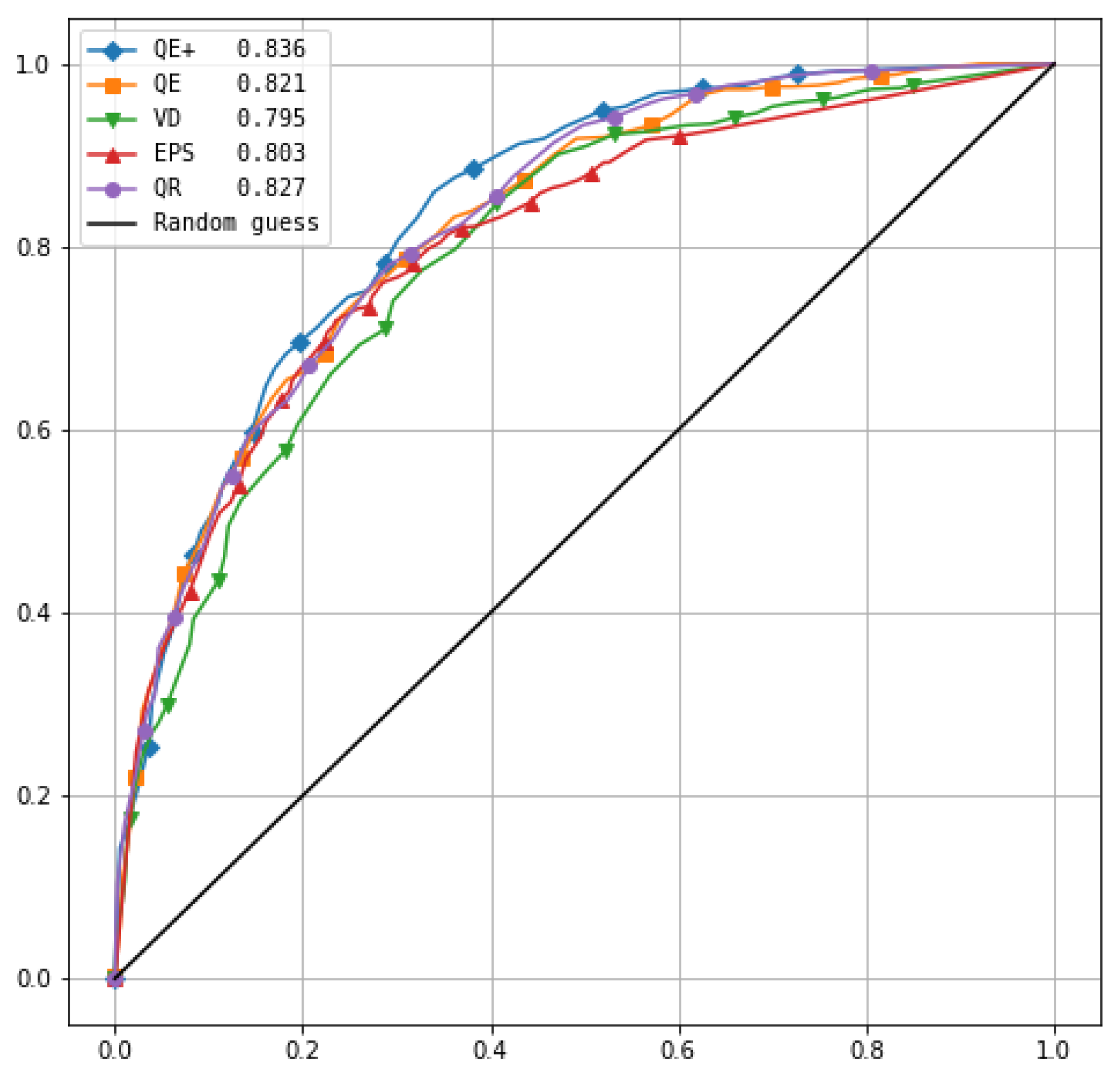
A graphical representation of the performance of the methods as binary classifiers with respect to the fixed threshold can be obtained by means of the ROC curves. In this plot, the false positives in the abscissa and the true positives in the ordinate are reported; the average results of the ensembles are represented as curves. The diagonal of the graph corresponds to a random guess on exceeding the threshold, and the ideal behavior is that for which there are very few false positives and the resulting curve is close to the axis of the ordinates. Figure 3 shows the ROC curves of the methods considered for exceeding the threshold equal to half the theoretical clear sky power and for a forecast lead time in the 24–48-h range. The area under the curve is a measure of the approximation of the ideal classifier behavior; the value is 0.5 for a random guess and tends to the unit under ideal conditions. Table 5 reports the values of the Area Under the Curve (AUC). The values in the table and the analysis of the curves in Figure 3 confirm the results obtained with the Brier score analysis, showing very satisfactory results for the QR method and for the QE and QE+ methods. The results with the QE method are better than those obtained with both the uncalibrated EPS and VD method, but the AUC value is lower than the result obtained with QR for a lead time up to 24 h. The QE+ method takes advantage of the use of IFS forecast information and is superior to other methods for forecast times greater than 24 h. In very short forecast times, the QR procedure still allows for better results.
The most significant score for the evaluation of the quality of a probabilistic forecast of a continuous variable is represented by the CRPS, which evaluates the quality of the forecast without the need to define a threshold. Table 5 reports the values of this measure for the methods considered and for the three forecast days. On the first and second day, the methods based on the use of the IFS forecast have a clear advantage over the others. In fact, the QR method applied to the IFS guarantees more than satisfactory performance up to a horizon of 48 h. On the third day of forecast, the importance of using EPS data emerges, provided the good calibration of the ensemble; the best results are in fact achieved with the QE and QE+ methods, the latter ensuring good and balanced performance over the entire forecast interval.
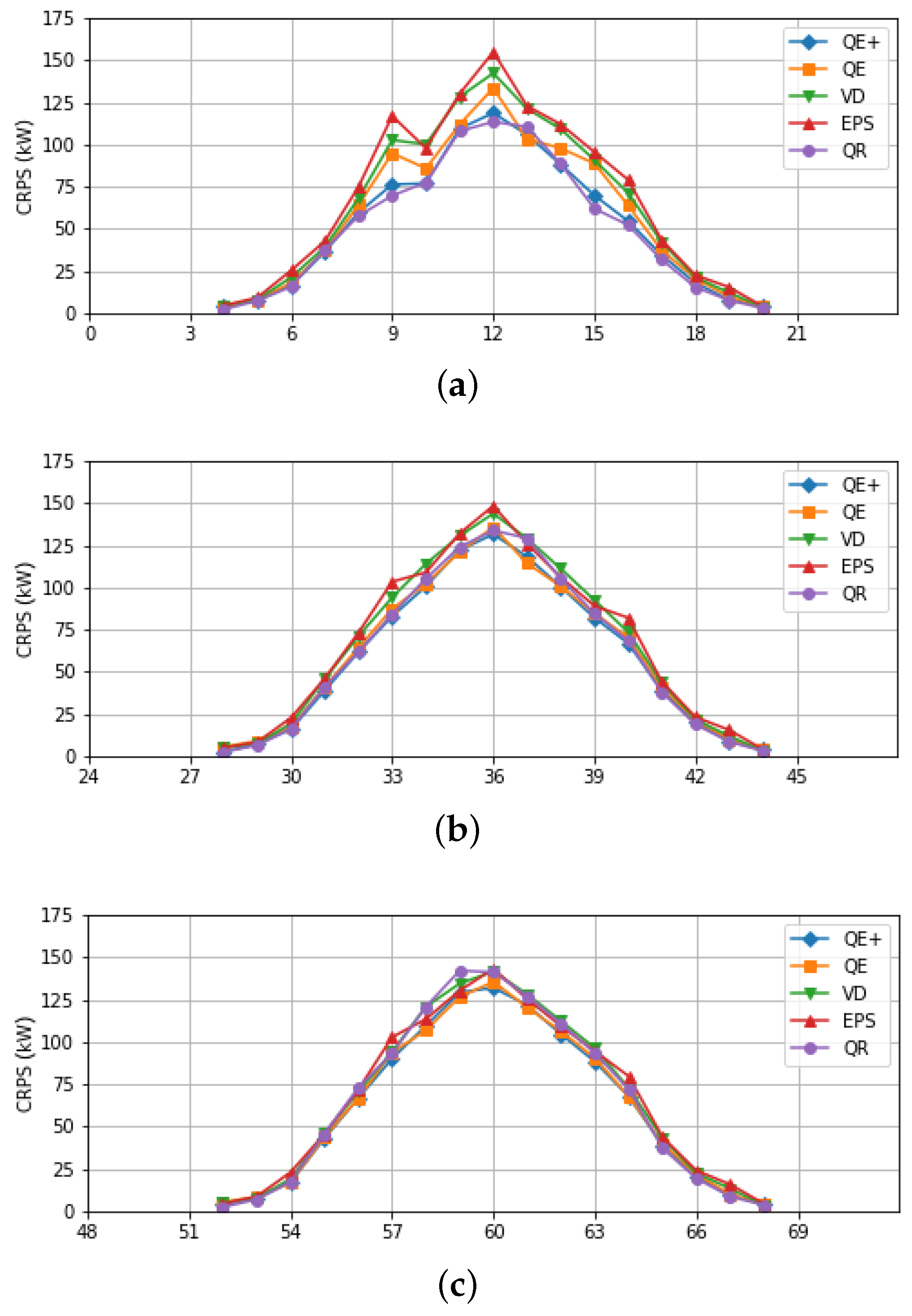
It may be interesting to evaluate the CRPS over the entire forecast interval for each daylight hour. The result is shown in Figure 4, which confirms the good performance of QE+, the more than satisfactory performance of the QR method for shorter forecast times and also its worse performance for longer horizons.
The QE+ method allows for improvements in deterministic forecasting, as well. Table 6 reports the performances obtained using as estimation of the power generated, the median of the ensembles produced by QE+ for each forecast time of the test period and for the three lead times. Comparison with the results shown in Table 4 shows a reduction in error compared to the performance obtained with deterministic forecast; the improvement increases with lead time and becomes relevant on the third day of forecast.
5. Discussion
In this work, we proposed a probabilistic forecast methodology that uses both the IFS and EPS forecasts of the ECMWF model, realizing a forecast with hourly resolution with a horizon of up to three days. It is difficult to compare the accuracy of the forecast obtained with the proposed methodology with the results available in the literature, due to the specificity of the plants and the different climatic conditions that characterize each installation site. We limit ourselves to the results of recent work, so that the basic meteorological model has comparable accuracy, and to installations on the European continent, so that climatic conditions may not be too dissimilar.
A measure that can be indicative of the quality of the deterministic forecast is represented by the skill score with respect to the RMSE error, which provides a measure of the reduction of the forecast error with respect to a forecast based on persistence alone. For example, in [10] an nRMSE of 10.14% was obtained for a plant located in Spain in the first day of the forecast and a skill score of 36.3%, with climatic conditions more favorable to photovoltaic production than the plant examined, located in northern Germany. Unfortunately, their discussion of probability forecasting results does not use any standard metrics and is therefore not directly comparable to our results. In [12], the proposed methodology had a skill score between 33% and 36% depending on the plant examined, for five plants located in northern Spain. The hourly forecast for a 662 kW plant in Northern Italy was evaluated at [15] using several forecasting techniques and an ensemble of the forecasts obtained from these models. The individual models produced skill scores between 35% and 42%, while the use of the ensemble of models technique made it possible to achieve a score of 46%. The values we have obtained are above 43% for the day-ahead hourly forecast. The use of an ensemble of regression models to further increase this score is a possible development for the methodology we have proposed.
Comparing the performance of the probabilistic forecast with the results of the literature is even more difficult due to the fact that very few works use standard metrics for performance evaluation, and in particular, the CRPS metric. In [16], the EPS forecast of the ECMWF is calibrated with two different methodologies and is used to forecast the day-ahead power generation for three plants in different locations in Italy. Their forecast has a resolution of 3 h, as that of the EPS, and not 1 h as that obtained with our procedure. Unfortunately, the CRPS is not calculated for the entire dataset, but its peak value relative to the nominal power of the plants is reported.
Peak values occur at noon and are about 8–9% of the rated power for the three installations and for both calibration methods presented. The forecast obtained with the QE+ procedure was resampled and the three-hour average value computed to obtain a performance comparison. The peak of the CRPS for a forecast with 3-h resolution yielded a value of CRPS equal to 6.7%, 7.9% and 8.2% of the nominal power of the plant for the first, second and third day of the forecast. The forecast in [17] has a maximum lead time of 3 h and is relative to intervals and not to the forecast probability distribution. The next day’s probability forecast for three PV plants in Australia is presented in [18], which shows the advantage of using a combination of machine learning methods for greater accuracy. The error metric pinball loss is adopted in their work, and the authors in their conclusions refer to “the need” to evaluate the performance of the method with CRPS. The authors obtain a pinball loss of 0.014–0.015 for the three PV plants, with an evaluation of the error over the entire 24-h period. The equivalent loss for our installation with the QE+ procedure is 0.013, evaluated as the average of the loss function (14) for the test set and for all quantiles
6. Conclusions
In this paper, we have proposed a new methodology for the short-term probabilistic forecasting of solar power, based on the technique of quantile regression and on the post-processing of an ensemble of forecasts. The method was applied to a mid-range plant in northern Germany. The results of the IFS and EPS models of the ECMWF were used for the forecasts. The procedure was compared with a quantile regression-based forecast with the use of IFS forecast only, with an ensemble of forecasts based on EPS and with the EPS ensemble calibrated using the variance deficit procedure.
The results highlighted the different content of information that can be retrieved from the results of the ECMWF forecast, showing how the IFS model, with its higher temporal and spatial detail, can provide the best accuracy for forecast horizons up to 24 h. EPS’s usefulness emerges for longer forecast horizons and gains relevance from the third forecast day onwards.
Probabilistic forecast methods were compared using the rank histogram, the Brier score for exceeding a production threshold, through the ROC curve diagram and through the CRPS score. The procedure proposed through the joint use of the results of the IFS and EPS forecast of the ECMWF meteorological models allowed good results to be obtained over the entire forecast horizon examined.
The work will be developed applying this methodology also to the forecast of wind turbine power generation and to the forecast of the net grid load when there is significant production from renewable sources.
Author Contributions
The authors jointly conceived of and designed the methodologies, performed the analysis and wrote the paper.
Acknowledgments
This work was partially financed by the European Union’s Horizon 2020 research and innovation program under Grant Agreement No. 646463, project NETfficient, Energy and economic efficiency for today’s smart communities through integrated multi-storage technologies, which also covered the costs to publish in open access, by the project “Tessuto Digitale Metropolitano” funded by the ROP Sardegna ERDF Action 1.2.2 and by the Sardinian Regional Authorities.
Conflicts of Interest
The authors declare no conflict of interest. The founding sponsors had no role in the design of the study; in the collection, analyses or interpretation of data; in the writing of the manuscript; nor in the decision to publish the results.
Abbreviations
The following abbreviations are used in this manuscript:
| PF | Probabilistic Forecasting procedures |
| GBRT | Gradient-Boosted Regression Trees |
| PV | Photo-Voltaic |
| ECMWF | European Centre for Medium-Range Weather Forecasts |
| IFS | Integrated Forecasting System |
| EPS | Ensemble Prediction System |
| QR | Quantile Regression |
| VD | Variance Deficit |
| NWP | Numerical Weather Predictions |
| AnEn | Analog Ensemble |
| PeEn | Persistence Ensemble |
| WRF | Weather Research and Forecasting regional model |
| EMOS | Ensemble Model Output Statistics |
| QE | Quantile Ensemble |
| QE+ | Quantile Ensemble Plus |
| DNI | Direct Normal Irradiation |
| DHI | Diffuse Horizontal Irradiation |
| GHI | Global Horizontal Irradiation |
| POA | Plane Of Array |
| RTM | Radiative Transfer Models |
| CF | Control Forecast |
| ME | Mean Error |
| MAE | Mean Absolute Error |
| RMSE | Root Mean Square Error |
| nME | normalized Mean Error |
| nMAE | normalized Mean Absolute Error |
| nRMSE | normalized Root Mean Square Error |
| SS | Skill Score |
| ROC | Receiver Operating Characteristic |
| AUC | Area Under the ROC Curve |
| BS | Brier Score |
| UNC | Uncertainty |
| REL | Reliability |
| RES | Resolution |
| CRPS | Continuous Ranked Probability Score |
| CDF | Cumulative Distribution Function |
References
- Kraas, B.; Schroedter-Homscheidt, M.; Madlener, R. Economic merits of a state-of-the-art concentrating solar power forecasting system for participation in the Spanish electricity market. Solar Energy 2013, 93, 244–255. [Google Scholar] [CrossRef]
- Luoma, J.; Mathiesen, P.; Kleissl, J. Forecast value considering energy pricing in California. Appl. Energy 2014, 125, 230–237. [Google Scholar] [CrossRef]
- Nonnenmacher, L.; Kaur, A.; Coimbra, C.F. Day-ahead resource forecasting for concentrated solar power integration. Renew. Energy 2016, 86, 866–876. [Google Scholar] [CrossRef]
- Yuan, S.; Kocaman, A.S.; Modi, V. Benefits of forecasting and energy storage in isolated grids with large wind penetration—The case of Sao Vicente. Renew. Energy 2017, 105, 167–174. [Google Scholar] [CrossRef]
- Hong, T.; Pinson, P.; Fan, S.; Zareipour, H.; Troccoli, A.; Hyndman, R.J. Probabilistic energy forecasting: Global Energy Forecasting Competition 2014 and beyond. Int. J. Forecast. 2016, 32, 896–913. [Google Scholar] [CrossRef] [Green Version]
- Antonanzas, J.; Osorio, N.; Escobar, R.; Urraca, R.; Martinez-de Pison, F.; Antonanzas-Torres, F. Review of photovoltaic power forecasting. Solar Energy 2016, 136, 78–111. [Google Scholar] [CrossRef]
- Van der Meer, D.; Widén, J.; Munkhammar, J. Review on probabilistic forecasting of photovoltaic power production and electricity consumption. Renew. Sustain. Energy Rev. 2017, 81, 1484–1512. [Google Scholar] [CrossRef]
- Bacher, P.; Madsen, H.; Nielsen, H.A. Online short-term solar power forecasting. Solar Energy 2009, 83, 1772–1783. [Google Scholar] [CrossRef] [Green Version]
- Lorenz, E.; Hurka, J.; Heinemann, D.; Beyer, H.G. Irradiance forecasting for the power prediction of grid-connected photovoltaic systems. IEEE J. Sel. Top. Appl. Earth Obs. Remote Sens. 2009, 2, 2–10. [Google Scholar] [CrossRef]
- Monteiro, C.; Santos, T.; Fernandez-Jimenez, L.A.; Ramirez-Rosado, I.J.; Terreros-Olarte, M.S. Short-term power forecasting model for photovoltaic plants based on historical similarity. Energies 2013, 6, 2624–2643. [Google Scholar] [CrossRef]
- Bracale, A.; Caramia, P.; Carpinelli, G.; Di Fazio, A.R.; Ferruzzi, G. A Bayesian method for short-term probabilistic forecasting of photovoltaic generation in smart grid operation and control. Energies 2013, 6, 733–747. [Google Scholar] [CrossRef]
- Almeida, M.P.; Perpiñán, O.; Narvarte, L. PV power forecast using a nonparametric PV model. Solar Energy 2015, 115, 354–368. [Google Scholar] [CrossRef] [Green Version]
- Alessandrini, S.; Delle Monache, L.; Sperati, S.; Cervone, G. An analog ensemble for short-term probabilistic solar power forecast. Appl. Energy 2015, 157, 95–110. [Google Scholar] [CrossRef] [Green Version]
- Huang, J.; Perry, M. A semi-empirical approach using gradient boosting and k-nearest neighbors regression for GEFCom2014 probabilistic solar power forecasting. Int. J. Forecast. 2016, 32, 1081–1086. [Google Scholar] [CrossRef]
- Pierro, M.; Bucci, F.; De Felice, M.; Maggioni, E.; Moser, D.; Perotto, A.; Spada, F.; Cornaro, C. Multi-Model Ensemble for day ahead prediction of photovoltaic power generation. Solar Energy 2016, 134, 132–146. [Google Scholar] [CrossRef]
- Sperati, S.; Alessandrini, S.; Delle Monache, L. An application of the ECMWF Ensemble Prediction System for short-term solar power forecasting. Solar Energy 2016, 133, 437–450. [Google Scholar] [CrossRef] [Green Version]
- Rana, M.; Koprinska, I. Neural network ensemble based approach for 2D-interval prediction of solar photovoltaic power. Energies 2016, 9, 829. [Google Scholar] [CrossRef]
- Ahmed Mohammed, A.; Aung, Z. Ensemble learning approach for probabilistic forecasting of solar power generation. Energies 2016, 9, 1017. [Google Scholar] [CrossRef]
- Owens, R.G.; Hewson, T.D. ECMWF Forecast User Guide; Technical Report; European Centre for Medium-Range Weather Forecasts: Reading, UK, 2018. [Google Scholar]
- Kopp, G.; Lean, J.L. A new, lower value of total solar irradiance: Evidence and climate significance. Geophys. Res. Lett. 2011, 38. [Google Scholar] [CrossRef] [Green Version]
- Inman, R.H.; Pedro, H.T.; Coimbra, C.F. Solar forecasting methods for renewable energy integration. Prog. Energy Combust. Sci. 2013, 39, 535–576. [Google Scholar] [CrossRef]
- Goswami, D.Y.; Kreith, F.; Kreider, J.F. Principles of Solar Engineering; CRC Press: Boca Raton, FL, USA, 2000. [Google Scholar]
- Ineichen, P.; Perez, R. A new airmass independent formulation for the Linke turbidity coefficient. Solar Energy 2002, 73, 151–157. [Google Scholar] [CrossRef] [Green Version]
- Ineichen, P. Comparison of eight clear sky broadband models against 16 independent data banks. Solar Energy 2006, 80, 468–478. [Google Scholar] [CrossRef]
- Rigollier, C.; Bauer, O.; Wald, L. On the clear sky model of the ESRA—European Solar Radiation Atlas—With respect to the Heliosat method. Solar Energy 2000, 68, 33–48. [Google Scholar] [CrossRef]
- Massidda, L.; Marrocu, M. Use of Multilinear Adaptive Regression Splines and numerical weather prediction to forecast the power output of a PV plant in Borkum, Germany. Solar Energy 2017, 146, 141–149. [Google Scholar] [CrossRef]
- Friedman, J.H. Greedy function approximation: a gradient boosting machine. Ann. Stat. 2001, 29, 1189–1232. [Google Scholar] [CrossRef]
- Pedregosa, F.; Varoquaux, G.; Gramfort, A.; Michel, V.; Thirion, B.; Grisel, O.; Blondel, M.; Prettenhofer, P.; Weiss, R.; Dubourg, V.; et al. Scikit-learn: Machine learning in Python. J. Mach. Learn. Res. 2011, 12, 2825–2830. [Google Scholar]
- Pinson, P. Very-short-term probabilistic forecasting of wind power with generalized logit–normal distributions. J. R. Stat. Soci. Ser. C (Appl. Stat.) 2012, 61, 555–576. [Google Scholar] [CrossRef]
- Taillardat, M.; Mestre, O.; Zamo, M.; Naveau, P. Calibrated ensemble forecasts using quantile regression forests and ensemble model output statistics. Mon. Weather Rev. 2016, 144, 2375–2393. [Google Scholar] [CrossRef]
- McKinney, W. Data structures for statistical computing in python. In Proceedings of the 9th Python in Science Conference, Austin, TX, USA, 28 June–3 July 2010; Volume 445, pp. 51–56. [Google Scholar]
- Holmgren, W.F.; Groenendyk, D.G. An open source solar power forecasting tool using PVLIB-Python. In Proceedings of the 2016 IEEE 43rd Photovoltaic Specialists Conference on Photovoltaic Specialists Conference (PVSC), Portland, OR, USA, 5–10 June 2016; pp. 972–975. [Google Scholar]
- Murphy, A.H. Skill scores based on the mean square error and their relationships to the correlation coefficient. Mon. Weather Rev. 1988, 116, 2417–2424. [Google Scholar] [CrossRef]
- Wilks, D.S. Statistical Methods in the Atmospheric Sciences; Academic Press: Cambridge, MA, USA, 2011; Volume 100. [Google Scholar]
- Murphy, A.H. A new vector partition of the probability score. J. Appl. Meteorol. 1973, 12, 595–600. [Google Scholar] [CrossRef]
- Hersbach, H. Decomposition of the continuous ranked probability score for ensemble prediction systems. Weather Forecast. 2000, 15, 559–570. [Google Scholar] [CrossRef]
Figure 1.
Flowchart showing the steps required to realize the QE and QE+ forecast starting from the EPS and IFS power forecasts.
Figure 1.
Flowchart showing the steps required to realize the QE and QE+ forecast starting from the EPS and IFS power forecasts.

Figure 2.
Rank histograms for forecast ensembles produced by the five methods examined for the 24–48-h forecast horizon: (a) Quantile regression; (b) Uncalibrated EPS (full scale); (c) Uncalibrated EPS; (d) EPS with variance deficit calibration; (e) Quantile ensemble with EPS forecast; (f) Quantile ensemble with IFS and EPS forecasts. The calibration of the EPS method is not satisfactory, and the VD method has a better performance. The QR and QE methods show a good calibration.

Figure 3.
ROC curves for a threshold equal to half the clear sky power and for a forecast interval of 24–48 h. In the legend within the figure, the values of the area under the curve are also shown.
Figure 3.
ROC curves for a threshold equal to half the clear sky power and for a forecast interval of 24–48 h. In the legend within the figure, the values of the area under the curve are also shown.

Figure 4.
CRPS results as the lead time forecast varies for the probabilistic forecast methods examined: (a) CRPS values for times of forecast in 0–24-h time range; (b) same as before for 24–48-h; (c) same for 48–72-h.
Figure 4.
CRPS results as the lead time forecast varies for the probabilistic forecast methods examined: (a) CRPS values for times of forecast in 0–24-h time range; (b) same as before for 24–48-h; (c) same for 48–72-h.


Table 1.
PV power output of the plant with 15-min resolution for 2014.
| Jan–Feb | Mar–Apr | May–Jun | Jul–Aug | Sep–Oct | Nov–Dec | Total | |
|---|---|---|---|---|---|---|---|
| Samples (-) | 5664 | 5856 | 5856 | 5952 | 5856 | 5856 | 35,040 |
| mean value (kW) | 68.4 | 204.2 | 261.6 | 276.5 | 150.3 | 49.1 | 169.2 |
| std. deviation (kW) | 161.8 | 309.1 | 344.0 | 361.3 | 262.2 | 128.2 | 289.9 |
| max value (kW) | 957.4 | 1187.9 | 1326.0 | 1276.2 | 1111.5 | 824.0 | 1326.0 |
Table 2.
Algorithm parameters tuned with grid search and 3-fold cross-validation.
| Parameter | Search Values | Deterministic | QE | QE+ |
|---|---|---|---|---|
| learning rate | 0.05, 0.02, 0.01 | 0.05 | 0.05 | 0.01 |
| maximum depth of trees | 3, 4, 5 | 3 | 3 | 3 |
| minimum number of samples in leaf | 3, 5, 7 | 7 | 7 | 5 |
| number of estimators | 100, 200, 500 | 100 | 200 | 500 |
Table 3.
Feature importance as the relative occurrence of the feature in the GBRT regression trees for the prediction of .
Table 3.
Feature importance as the relative occurrence of the feature in the GBRT regression trees for the prediction of .
| Feature | Relative Importance |
|---|---|
| k | 56.9% |
| Precipitation | 3.9% |
| Temperature 2 m | 11.3% |
| Zenith | 9.5 % |
| Azimuth | 18.4 % |
Table 4.
Error measures for the deterministic forecast based on the IFS model.
| Forecast (h) | R2 (-) | ME (kW) | MAE (kW) | RMSE (kW) | nMAE (%) | nRMSE (%) | SS(%) |
|---|---|---|---|---|---|---|---|
| 0–24 | 0.785 | 93.3 | 146.4 | 7.18 | 11.26 | 43.61 | |
| 24–48 | 0.687 | 6.9 | 114.3 | 176.5 | 8.80 | 13.57 | 35.62 |
| 48–72 | 0.636 | 7.5 | 124.8 | 190.4 | 9.60 | 14.65 | 27.78 |
Table 5.
Probabilistic error measures with different forecast lead times. The Brier Score (BS), its components reliability (REL), Resolution (RES) and Uncertainty (UNC) and the Area Under the ROC Curve (AUC) are calculated for a threshold of . The cumulative ranked probability score is the mean value for the test set in the daylight hours only.
| Forecast (h) | Model | BS (-) | REL (-) | RES (-) | UNC (-) | AUC (-) | CRPS (kW) |
|---|---|---|---|---|---|---|---|
| 0–24 | QR | 0.140 | 0.008 | 0.117 | 0.249 | 0.882 | 65.7 |
| EPS | 0.204 | 0.043 | 0.089 | 0.249 | 0.814 | 87.5 | |
| VD | 0.179 | 0.014 | 0.085 | 0.249 | 0.808 | 82.3 | |
| QE | 0.162 | 0.006 | 0.094 | 0.249 | 0.845 | 74.9 | |
| QE+ | 0.143 | 0.006 | 0.113 | 0.249 | 0.876 | 67.7 | |
| 24–48 | QR | 0.170 | 0.008 | 0.087 | 0.249 | 0.827 | 79.2 |
| EPS | 0.199 | 0.027 | 0.077 | 0.249 | 0.803 | 86.3 | |
| VD | 0.188 | 0.012 | 0.074 | 0.249 | 0.794 | 85.3 | |
| QE | 0.173 | 0.007 | 0.083 | 0.249 | 0.821 | 78.4 | |
| QE+ | 0.165 | 0.007 | 0.091 | 0.249 | 0.836 | 76.8 | |
| 48–72 | QR | 0.184 | 0.007 | 0.073 | 0.249 | 0.800 | 85.9 |
| EPS | 0.199 | 0.026 | 0.077 | 0.249 | 0.796 | 86.2 | |
| VD | 0.191 | 0.014 | 0.072 | 0.249 | 0.789 | 86.3 | |
| QE | 0.176 | 0.006 | 0.079 | 0.249 | 0.815 | 81.2 | |
| QE+ | 0.172 | 0.008 | 0.086 | 0.249 | 0.825 | 80.7 |
Values in bold are relative to the best performance for each of the indicators.
Table 6.
Error measures for the deterministic forecast based on the median of the quantile ensemble probabilistic model with the IFS and EPS forecasts.
Table 6.
Error measures for the deterministic forecast based on the median of the quantile ensemble probabilistic model with the IFS and EPS forecasts.
| Forecast (h) | R2 (-) | ME (kW) | MAE (kW) | RMSE (kW) | nMAE (%) | nRMSE (%) | SS (%) |
|---|---|---|---|---|---|---|---|
| 0–24 | 0.784 | −5.1 | 93.5 | 146.8 | 7.19 | 11.29 | 43.46 |
| 24–48 | 0.721 | 0.6 | 110.0 | 166.7 | 8.46 | 12.82 | 39.18 |
| 48–72 | 0.704 | 0.7 | 117.1 | 171.6 | 9.00 | 13.20 | 34.92 |
© 2018 by the authors. Licensee MDPI, Basel, Switzerland. This article is an open access article distributed under the terms and conditions of the Creative Commons Attribution (CC BY) license (http://creativecommons.org/licenses/by/4.0/).
Share and Cite
MDPI and ACS Style
Massidda, L.; Marrocu, M. Quantile Regression Post-Processing of Weather Forecast for Short-Term Solar Power Probabilistic Forecasting. Energies 2018, 11, 1763. https://doi.org/10.3390/en11071763
AMA Style
Massidda L, Marrocu M. Quantile Regression Post-Processing of Weather Forecast for Short-Term Solar Power Probabilistic Forecasting. Energies. 2018; 11(7):1763. https://doi.org/10.3390/en11071763
Chicago/Turabian StyleMassidda, Luca, and Marino Marrocu. 2018. "Quantile Regression Post-Processing of Weather Forecast for Short-Term Solar Power Probabilistic Forecasting" Energies 11, no. 7: 1763. https://doi.org/10.3390/en11071763
Note that from the first issue of 2016, this journal uses article numbers instead of page numbers. See further details here.